TinyMPC: Model-Predictive Control on
Resource-Constrained Microcontrollers

Abstract

Model-predictive control (MPC) is a powerful tool for controlling highly dynamic robotic systems subject to complex constraints. However, MPC is computationally demanding, and is often impractical to implement on small, resource-constrained robotic platforms. We present TinyMPC, a high-speed MPC solver with a low memory footprint targeting the microcontrollers common on small robots. Our approach is based on the alternating direction method of multipliers (ADMM) and leverages the structure of the MPC problem for efficiency. We demonstrate TinyMPC both by benchmarking against the state-of-the-art solver OSQP, achieving nearly an order of magnitude speed increase, as well as through hardware experiments on a 27 g quadrotor, demonstrating high-speed trajectory tracking and dynamic obstacle avoidance.

I Introduction

Model-predictive control (MPC) enables reactive and dynamic online control for robots while respecting complex control and state constraints such as those encountered during dynamic obstacle avoidance and contact events [1, 2, 3, 4]. However, despite MPC’s many successes, its practical application is often hindered by computational limitations, which can necessitate algorithmic simplifications [5, 6]. This challenge is amplified when dealing with systems that have fast or unstable open-loop dynamics, where high control rates are needed for safe and effective operation.

At the same time, there has been an explosion of interest in tiny, low-cost robots that can operate in confined spaces, making them a promising solution for applications ranging from emergency search and rescue [7] to routine monitoring and maintenance of infrastructure and equipment [8, 9]. These robots are limited to low-power, resource-constrained microcontrollers (MCUs) for their computation [10, 11]. As shown in Figure 2, these microcontrollers feature orders of magnitude less processor speed, RAM ,and flash memory compared to the CPUs and GPUs available on larger robots and, historically, were not able to support the real-time execution of computationally or memory-intensive algorithms [12, 13]. Consequently, many of the examples in the literature of intelligent robot behaviors being executed on these tiny platforms rely on off-board computers [14, 15, 16, 17, 18, 19, 20, 21, 22, 23, 24, 25].

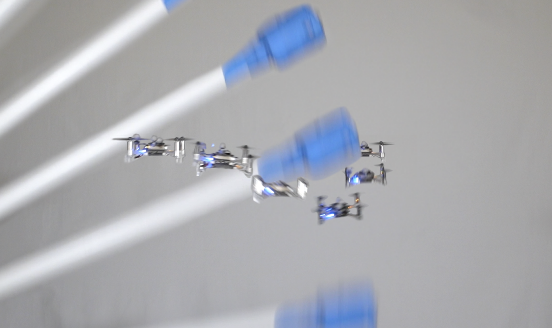
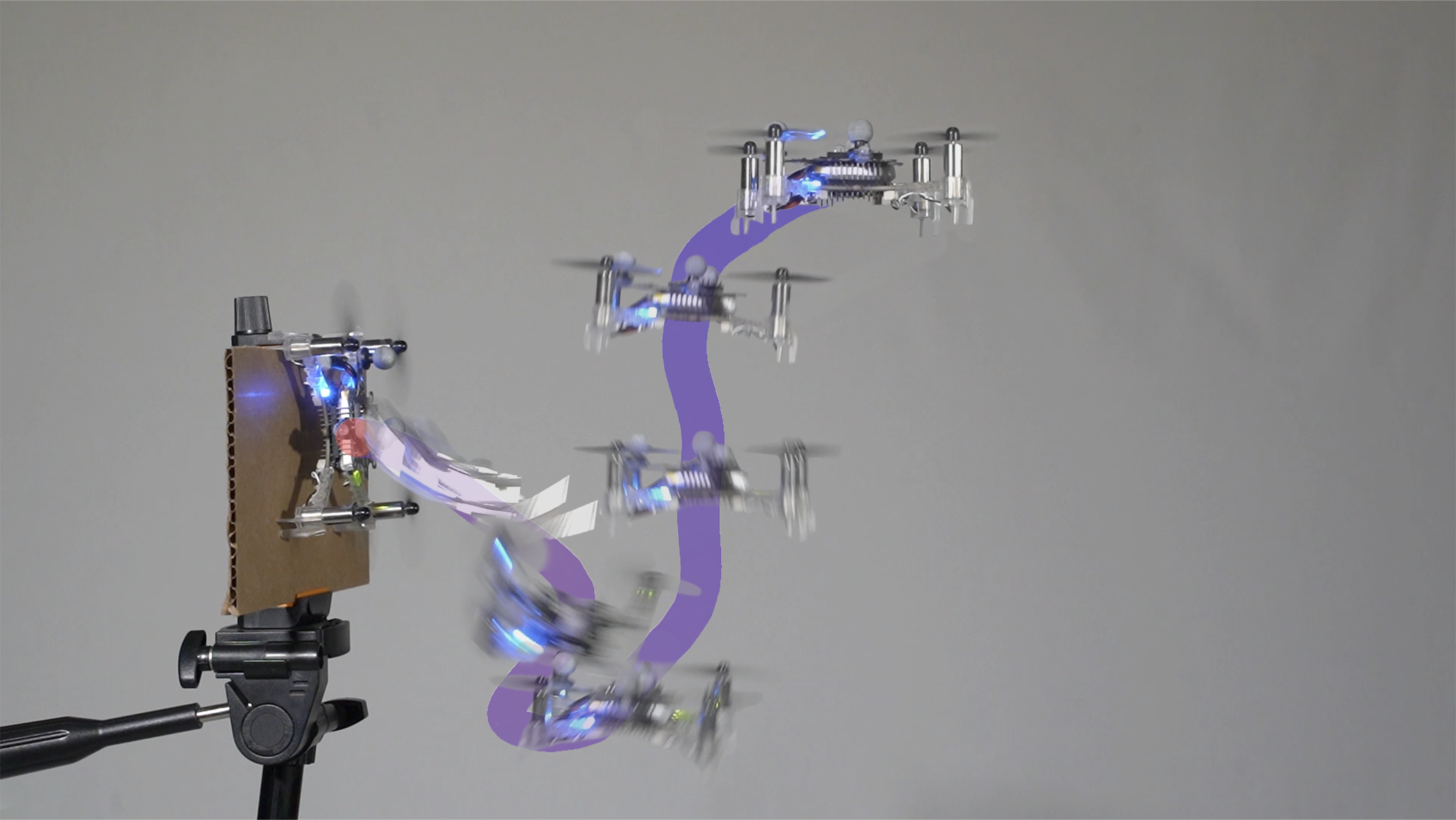
Figure 1: TinyMPC is a fast convex MPC solver that enables real-time optimal control on resource-constrained microcontrollers. We demonstrate its efficacy by performing dynamic obstacle avoidance (top) and recover from $90^{\circ}$ attitude errors (bottom) on a 27 g Crazyflie 2.1 quadrotor.

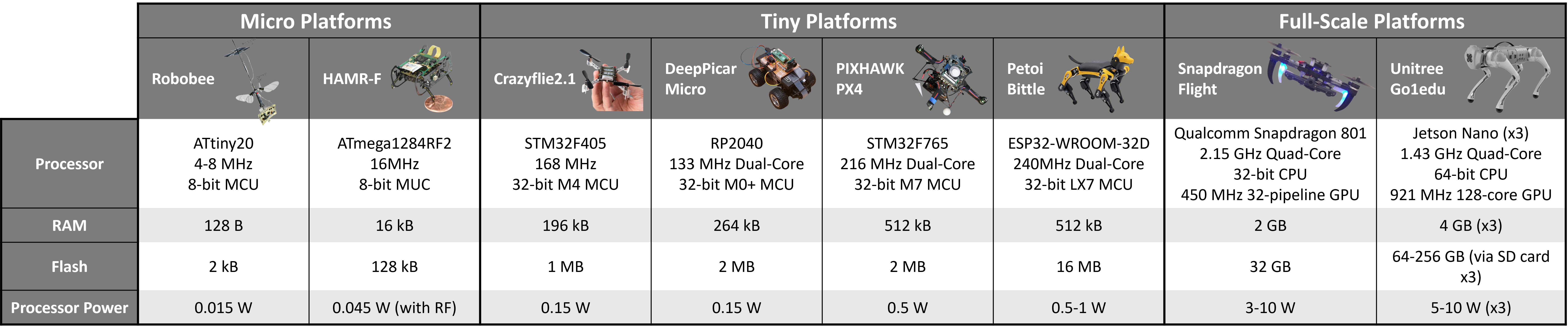
Figure 2: A comparison of micro, tiny, and full-scale robot platforms and their associated computational hardware. At the smallest scale, microrobots like the Robobee [26] and HAMR-F [27] use highly constrained 8-bit microcontrollers to execute pre-planned open-loop cyclical gates and wing motions. At large scales, powerful embedded CPUs and GPUs, found onboard the Snapdragon Flight quadrotor [28] or Unitree Go1edu quadruped [29], enable high performance at the cost of high power requirements. In this work we target tiny robots such as the Crazyflie2.1 [30], DeepPiCarMicro [31], PIXHAWK PX4 [32], and Petoi Bittle [33] that leverage 32-bit microcontrollers for motion planning and control. These devices are capable of some onboard computation, but feature orders of magnitude less processor speed, as well as RAM and flash memory, than the powerful large-scale embedded CPUs and GPUs.

Several efficient optimization solvers suitable for embedded MPC have emerged in recent years, most notably OSQP [34] and CVXGEN [35]. Both of these solvers have code-generation tools that enable users to create dependency-free C code to solve quadratic programs (QPs) on embedded computers. However, they do not take full advantage of the unique structure of the MPC problem and still have relatively large memory footprints, making them unable to run within the resource constraints of many microcontrollers.

Inspired by the recent success of “TinyML,” which has enabled the deployment of neural networks on microcontrollers [12], we introduce TinyMPC, an MCU-optimized implementation of convex MPC using the alternating direction method of multipliers (ADMM) algorithm. Our approach leverages the structure of the MPC problem by precomputing and caching as much as possible and completely avoiding divisions and matrix inversions online. This approach facilitates rapid computation and has a very small memory footprint, enabling deployment onto resource-constrained MCUs. To the best of the authors’ knowledge, TinyMPC is the first MPC solver tailored for execution on MCUs that has been demonstrated onboard a highly dynamic, compute-limited robotic system.

Our contributions include:

• A novel quadratic programming algorithm that: is optimized for MPC, is matrix-inversion free, and achieves high efficiency and a very low memory footprint. This combination makes it suitable for deployment on resource-constrained microcontrollers.

• An open-source solver implementation of TinyMPC in C++ that delivers state-of-the-art real-time performance for convex MPC problems on microcontrollers.

• Experimental demonstration on a small, resource-constrained agile quadrotor platform.

This paper proceeds as follows: Section II reviews linear-quadratic optimal control, convex optimization, and ADMM. Section III then derives the core TinyMPC solver algorithm. Benchmarking results and hardware experiments on a Crazyflie quadrotor are presented in Section IV. Finally, we summarize our results and conclusions in Section V.

II Background

II-A The Linear-Quadratic Regulator

The linear-quadratic regulator (LQR) [36] is a widely used approach for solving robotic control problems. LQR optimizes a quadratic cost function subject to a set of linear dynamics constraints:

$$\begin{split}\min_{\begin{subarray}{c}x_{1:N},u_{1:N-1}\end{subarray}}&J=\frac{1}{2}x_{N}^{\intercal}Q_{f}x_{N}+q_{f}^{\intercal}x_{N}+\\ \sum_{k=1}^{N-1}&\frac{1}{2}x_{k}^{\intercal}Qx_{k}+q_{k}^{\intercal}x_{k}+\frac{1}{2}u_{k}^{\intercal}Ru_{k}+r_{k}^{\intercal}u_{k}\\ \textrm{subject to}\quad&x_{k+1}=Ax_{k}+Bu_{k}\quad\forall k\in[1,N),\\ \end{split}$$ (1)

where $x_{k}\in\mathbb{R}^{n}$ $u_{k}\in\mathbb{R}^{m}$ are the state and control input at time step $k$, $N$ is the number of time steps (also referred to as the horizon), $A\in\mathbb{R}^{n\times n}$ and $B\in\mathbb{R}^{n\times m}$ define the system dynamics, $Q\succeq 0$, $R\succ 0$, and $Q_{f}\succeq 0$ are symmetric cost weight matrices and $q$ and $r$ are the linear cost vectors.

Equation (1) has a closed-form solution in the form of a linear feedback controller [36]:

$$u_{k}^{*}=-K_{k}x_{k}-d_{k},$$ (2)

$K_{k}$ and $d_{k}$ can be obtained by solving the discrete Riccati equation backwards in time, starting with $P_{N}=Q_{f}$ and $p_{N}=q_{f}$, where $P_{k}$ and $p_{k}$ are the Hessian and linear terms of the cost-to-go (or value) function [36]:

$$\begin{split}K_{k}&=(R+B^{\intercal}P_{k+1}B)^{-1}(B^{\intercal}P_{k+1}A)\\ d_{k}&=(R+B^{\intercal}P_{k+1}B)^{-1}(B^{\intercal}p_{k+1}+r_{k})\\ P_{k}&=Q+K_{k}^{\intercal}RK_{k}+(A-BK_{k})^{\intercal}P_{k+1}(A-BK_{k})\\ p_{k}&=q_{k}+(A-BK_{k})^{\intercal}(p_{k+1}-P_{k+1}Bd_{k})+\\ &\qquad K_{k}^{\intercal}(Rd_{k}-r_{k}).\end{split}$$ (3)

II-B Convex Model-Predictive Control

Convex MPC extends the LQR formulation to admit additional convex constraints on the system states and control inputs such as joint and torque limits, hyperplanes for obstacle avoidance, and contact constraints:

$$\min_{x_{1:N},u_{1:N-1}} J(x_{1:N},u_{1:N-1})$$ (4)

subject to $$x_{k+1}=Ax_{k}+Bu_{k},$$

$$x_{k}\in\mathcal{X},u_{k}\in\mathcal{U},$$

where $\mathcal{X}$ and $\mathcal{U}$ are convex sets. The convexity of this problem means that it can be solved efficiently and reliably, enabling real-time deployment in a variety of control applications including the landing of rockets [37], legged locomotion [38], and autonomous driving [39].

When $\mathcal{X}$ and $\mathcal{U}$ can be expressed as linear equality or inequality constraints, (4) is a QP, and can be put into the standard form:

$$\min_{x\in\mathbb{R}^{n}} \frac{1}{2}x^{\intercal}Px+q^{\intercal}x$$ (5)

subject to $$Ax\leq b,$$

$$Cx=d.$$

II-C The Alternating Direction Method of Multipliers

The alternating direction method of multipliers (ADMM) [40, 41, 42] is a popular and efficient approach for solving convex optimization problems, including QPs like (5). We provide a very brief summary here and refer readers to [43] for more details.

Given a generic problem:

$$\min_{x} f(x)$$ (6)

subject to $$x\in\mathcal{C},$$

with $f$ and $\mathcal{C}$ convex, we define the indicator function for the set $\mathcal{C}$:

$$I_{\mathcal{C}}(z)=\begin{cases}0&z\in\mathcal{C}\\ \infty&\text{otherwise}.\end{cases}$$ (7)

We can now form the following equivalent problem by introducing the slack variable $z$:

$$\min_{x} f(x)+I_{\mathcal{C}}(z)$$ (8)

subject to $$x=z.$$

The augmented Lagrangian of the transformed problem (8) is as follows where $\lambda$ is a Lagrange multiplier and $\rho$ is a scalar penalty weight:

$$\mathcal{L}_{A}(x,z,\lambda)=f(x)+I_{\mathcal{C}}(z)+\lambda^{\intercal}(x-z)+\frac{\rho}{2}||x-z||_{2}^{2}.$$ (9)

If we alternate minimization over $x$ and $z$, rather than simultaneously minimizing over both, we arrive at the three-step ADMM iteration,

$$\text{primal update}:x^{+} =\operatorname*{arg\,min}_{x}\mathcal{L}_{A}(x,z,\lambda),$$ (10)

$$\text{slack update}:z^{+} =\operatorname*{arg\,min}_{z}\mathcal{L}_{A}(x^{+},z,\lambda),$$ (11)

$$\text{dual update}:\lambda^{+} =\lambda+\rho(x^{+}-z^{+}),$$ (12)

the last step of which is a dual-ascent update on the Lagrange multiplier [42]. These steps can be iterated until a desired convergence tolerance is achieved.

In the special case of a QP, each step of the ADMM algorithm becomes very simple to compute: the primal update is the solution to a linear system, and the dual update is a linear projection. ADMM-based QP solvers, like OSQP [34], have demonstrated state-of-the-art results.

III The TinyMPC Solver

TinyMPC trades generality for speed by exploiting the special structure of the MPC problem. Specifically, we leverage the closed-form Riccati solution to the LQR problem in the primal update of (10). Pre-computing and caching this solution allows us to avoid online matrix factorizations and enables very fast performance and a small memory footprint.

III-A Combining LQR and ADMM for MPC

We solve the following problem, introducing slack variables as in  (9) and transforming  (4) into the following:

$$\min_{{\begin{subarray}{c}x_{1:N},{z}_{1:N},{\lambda}_{1:N}\\ u_{1:N-1},{w}_{1:N-1},{\mu}_{1:N-1}\\ \end{subarray}}} \mathcal{L}_{A}(\cdot)=~{}J(x_{1:N},u_{1:N-1})+$$ (13)

$$I_{\mathcal{X}}({z}_{1:N})+I_{\mathcal{U}}({w}_{1:N-1})+$$

$$\sum_{k=1}^{N}\bigl{(}\frac{\rho}{2}(x_{k}-{z}_{k})^{\intercal}(x_{k}-{z}_{k})+$$

$$\quad\qquad{\lambda}_{k}^{\intercal}(x_{k}-{z}_{k})\bigr{)}+$$

$$\sum_{k=1}^{N-1}\bigl{(}\frac{\rho}{2}(u_{k}-{w}_{k})^{\intercal}(x_{k}-{w}_{k})+$$

$$\quad\qquad{\mu}_{k}^{\intercal}(u_{k}-{w}_{k})\bigr{)}$$

subject to $$x_{k+1}=Ax_{k}+Bu_{k},$$

where $z$, $w$, $\lambda$, $\mu$ are the state slack, input slack, state dual, and input dual variables over the entire horizon. The primal update for  (13) becomes an equality-constrained QP:

$$\min_{x_{1:N},u_{1:N-1}} \frac{1}{2}x_{N}^{\intercal}\tilde{Q}_{f}x_{N}+\tilde{q}_{f}^{\intercal}x_{N}+$$ (14)

$$\sum_{k=1}^{N-1} \frac{1}{2}x_{k}^{\intercal}\tilde{Q}x_{k}+\tilde{q}_{k}^{\intercal}x_{k}+\frac{1}{2}u_{k}^{\intercal}\tilde{R}x_{k}+\tilde{r}^{\intercal}u_{k}$$

subject to $$x_{k+1}=Ax_{k}+Bu_{k},$$

where

$$\tilde{Q}_{f}=Q_{f}+\rho I, \quad\tilde{q}_{f}=q_{f}+\lambda_{N}-\rho z_{N},$$ (15)

$$\tilde{Q}=Q+\rho I, \quad\tilde{q}_{k}=q_{k}+\lambda_{k}-\rho z_{k},$$

$$\tilde{R}=R+\rho I, \quad\tilde{r}_{k}=r_{k}+\mu_{k}-\rho w_{k}.$$

We leverage a scaled form of (17) by introducing the scaled dual variables $y$ and $g$ [42]:

$$\tilde{q}_{f}=q_{f}+\rho(\lambda_{N}/\rho-z_{N})=q_{f}+\rho(y_{N}-z_{N}),$$ (16)

$$\tilde{q}_{k}=q_{k}+\rho(\lambda_{k}/\rho-z_{k})=q_{k}+\rho(y_{k}-z_{k}),$$

$$\tilde{r}_{k}=r_{k}+\rho(\mu_{k}/\rho-w_{k})=r_{k}+\rho(g_{k}-w_{k}).$$

We observe that because (14) exhibits the same LQR problem structure as in (1), (14) can be solved with (3). The slack update for (13) becomes a simple linear projection onto the feasible set:

$$z^{+}_{k} =\operatorname{proj}_{\mathcal{X}}(x^{+}_{k}+y_{k})$$ (17)

$$w^{+}_{k} =\operatorname{proj}_{\mathcal{U}}(u^{+}_{k}+g_{k}).$$

Finally, the dual update for  (13) simply becomes

$$y^{+}_{k} =y_{k}+x^{+}_{k}-z^{+}_{k}$$ (18)

$$g^{+}_{k} =g_{k}+u^{+}_{k}-w^{+}_{k}.$$

Figure 3: Comparison of average iteration times (top) and memory usage (bottom) for OSQP and TinyMPC on randomly generated trajectory tracking problems on a Teensy 4.1 development board (ARM Cortex-M7 running at 600MHz with 32-bit floating point support, 7.75Mb of flash, and 512kB of tightly coupled RAM). Error bars show the maximum and minimum time per iteration over all MPC steps executed for a given problem. In (a), the input dimension and time horizon are held constant at $m=4$ and $N=10$ while the state dimension $n$ varies from 4 to 32. In (b), $n=10$ and $N=10$ while the $m$ varies from 4 to 32. In (c), $n=10,m=4$ and $N$ varies from 4 to 50. The dotted black line indicates the memory limit of the Teensy 4.1.

III-B Pre-Computation and Penalty Scaling

Solving the linear system in each primal update is the most expensive step in each ADMM iteration. In our case, this is the solution to the Riccati equation, which has properties we can leverage to significantly reduce computation and memory usage. Given a long enough horizon, the Riccati recursion (3) converges to the solution of the infinite-horizon LQR problem [36]. As such, we can pre-compute a single LQR gain matrix $K_{\text{inf}}$ and cost-to-go Hessian $P_{\text{inf}}$. We then cache the following matrices:

$$C_{1} =(R+B^{\intercal}P_{\text{inf}}B)^{-1}$$ (19)

$$C_{2} =(A-BK_{\text{inf}})^{\intercal}$$

$$C_{3} =K_{\text{inf}}^{\intercal}R-C_{2}P_{\text{inf}}B$$

A careful analysis of the Riccati equation then reveals that only the linear terms need to be updated as part of the ADMM iteration:

$$d_{k} =C_{1}(B^{\intercal}p_{k+1}+r_{k})$$ (20)

$$p_{k} =q_{k}+C_{2}p_{k+1}-K_{\text{inf}}^{\intercal}r_{k}+C_{3}d_{k}$$

As a result, we can completely avoid matrix factorizations online and only compute matrix-vector products using the pre-computed matrices.

ADMM is also sensitive to the value of the penalty term $\rho$ in (9). Adaptively scaling $\rho$ is standard in solvers like OSQP [34]. However, this requires additional matrix factorizations that we are trying to avoid. Therefore, we pre-compute and cache a set of matrices corresponding to several values of $\rho$. Online, we switch between these cached matrices according to the primal and dual residual values, in a scheme adapted from OSQP. The resulting TinyMPC algorithm is summarized in Algorithm 1.

Algorithm 1 TinyMPC

1:function TinyMPC(input)

2:     while not converged do

3:         $\triangleright$Primal update

4:         $p_{1:N-1},d_{1:N-1}\leftarrow\text{Backward pass via \eqref{eq:fast_riccati}}$

5:         $x_{1:N},u_{1:N-1}\leftarrow\text{Forward pass via \eqref{eq:lqrSolution}}$

6:         $\triangleright$Slack update

7:         $z_{1:N},w_{1:N-1}\leftarrow\text{Projected to feasible set \eqref{eq:mpc_slack}}$

8:         $\triangleright$Dual update

9:         $y_{1:N},g_{1:N-1}\leftarrow\text{Gradient ascent \eqref{eq:mpc_dual}}$

10:         $q_{1:N},r_{1:N-1},p_{N}\leftarrow\text{Update linear cost terms}$      return $x_{1:N},u_{1:N-1}$

IV Experiments

Figure 4: Control trajectories during the Extreme Initial Poses experiment. Four sets of pre-clipped PWM Motor commands, ranging from 0 to 65535, are shown for each controller. The black dotted line is the thrust limit. Among the three successful controllers, only TinyMPC can guarantee feasible controls.

Figure 5: Figure-eight tracking at low speed (top) and high speed (bottom) comparing TinyMPC with the two most performant available on the Crazyflie. For slower trajectories, all three controllers resulted in similar performance. For faster trajectories, only TinyMPC was capable of maintaining tracking without crashing. The maximum velocity and attitude deviation from hover with TinyMPC reached 1.5m/s and 20^∘, respectively.

We evaluate TinyMPC through two sets of experiments: First, we benchmark our solver against the state-of-the-art OSQP [34] solver on a representative microcontroller, demonstrating improved computational speed and reduced memory footprint. We then test the efficacy of our solver on a resource-constrained nano-quadrotor platform, the Crazyflie 2.1. We show that TinyMPC enables the Crazyflie to track aggressive reference trajectories while satisfying control limits and time-varying state constraints.

IV-A Microcontroller Benchmarks

We compare TinyMPC and OSQP on random linear MPC problems while varying the state and input dimensions as well as the horizon length.

IV-A1 Methodology

Experiments are performed on a Teensy 4.1 [44] development board, which has an ARM Cortex-M7 microcontroller operating at 600MHz, 7.75MB of flash memory, and 512kB of RAM. TinyMPC is implemented in C++ using the Eigen matrix library [45]. We leverage OSQP’s code-generation feature to generate a C implementation of our problem to run on the microcontroller. Wherever possible, solver parameters were set to equivalent values. Objective tolerances were set to $10^{-3}$ and constraint tolerances to $10^{-4}$. The maximum number of iterations for both solvers was set to 4000, and both utilized warm starting. OSQP’s solution polishing was disabled to make it faster. Dynamics models, $A$ and $B$, were randomly generated and checked to ensure controllability for all values of state dimension $n$, input dimension $m$, and time horizon $N$.

IV-A2 Evaluation

Fig. 3 shows the average execution times for both solvers, in which TinyMPC exhibits a maximum speed-up of 8.85x over OSQP. This speed-up allows TinyMPC to perform real-time trajectory tracking while handling input and state constraints. OSQP also quickly exceeded the memory limitations of the MCU, while TinyMPC was able to scale to much larger problem sizes. For example for a fixed input dimension of $m=4$ and time horizon of $N=10$, OSQP exceeds 512kB at only a state dimension of $n=16$, while TinyMPC only used around 400kB at a state dimension of $n=32$.

IV-B Hardware Experiments

We demonstrate the efficacy of our solver for real-time execution of dynamic control tasks on a resource-constrained Crazyflie 2.1 quadrotor. We present three experiments: 1) figure-eight trajectory tracking at slow and fast speeds, 2) recovery from extreme initial attitudes, and 3) dynamic obstacle avoidance through online updating of state constraints.

IV-B1 Methodology

The Crazyflie 2.1 is a 27 g quadrotor. Its main MCU is an ARM Cortex-M4 (STM32F405) clocked at 168MHz with 192kB of SRAM and 1MB of flash. OSQP could not fit within the memory available on this MCU. Instead, we compare against the four controllers shipped with the Crazyflie firmware: Cascaded PID [46], Mellinger [47], INDI [48], and Brescianini [49]. These are reactive controllers that often clip the control input to meet hardware constraints.

All experiments shown were performed in an OptiTrack motion capture environment sending pose data to the Crazyflie at 100 Hz. We ran TinyMPC at 500Hz with the horizon length $N=15$ for the figure-eight tracking task and the attitude-recovery task. For the obstacle-avoidance task, we sent the location of the end of a stick to the Crazyflie using the onboard radio. Additionally, we reduced the MPC frequency to 100 Hz and increased $N$ to 20. In all experiments, we linearize the quadrotor’s dynamics about a hover and represent its attitude with a quaternion using the formulation in [50]. We solve a problem with state dimension $n=12$ and $m=4$ for the Crazyflie’s full state pose and four PWM motor control commands.

IV-B2 Evaluation––Figure-Eight Trajectory Tracking

We compare the tracking performance of TinyMPC and other controllers with a figure-eight trajectory, as shown in Fig. 5. For the fast trajectory, the maximum velocity and attitude deviation reach 1.5 m/s and 20^∘, respectively. Only TinyMPC could track the entire reference, while the Mellinger and Brescianini controllers crashed almost immediately.

IV-B3 Evaluation––Extreme Initial Poses

Fig. 1 (bottom) shows the performance of the Crazyflie when initialized with a 90^∘ attitude error. TinyMPC displayed the best recovery performance with a maximum position error of 23 cm while respecting the input limits. The PID and Brescianini achieved maximum errors of 40 cm and 65 cm, respectively, while violating input limits (Fig. 4). The other controllers, INDI and Mellinger, failed to stabilize the quadrotor, causing it to crash.

IV-B4 Evaluation––Dynamic Obstacle Avoidance

We demonstrate TinyMPC’s ability to handle time-varying state constraints by avoiding a moving stick (Fig. 1 top). The obstacle constraint was re-linearized about its updated position at each MPC step, thereby allowing the drone to avoid the unplanned movements of the swinging stick. To make it more challenging, we add an additional constraint of the quadrotor’s moving within a vertical plane. While avoiding the dynamic obstacle, the Crazyflie only makes a maximum deviation of approximately 5 cm from the vertical plane.

V Conclusions

We introduce TinyMPC, a model-predictive control solver for resource-constrained embedded systems. TinyMPC uses ADMM to handle state and input constraints while leveraging the structure of the MPC problem and insights from LQR to reduce memory footprint and speed up online execution compared to existing state-of-the-art solvers like OSQP. We demonstrated TinyMPC’s practical performance on a Crazyflie nano-quadrotor performing highly dynamic tasks with input and obstacle constraints.

Several directions for future work remain: It should be straight-forward to extend TinyMPC to handle second-order cone constraints, which are useful in many MPC applications for modeling thrust and friction cone constraints. We also plan to further reduce TinyMPC’s hardware requirements by developing a fixed-point version, since many small microcontrollers lack hardware floating-point support. Finally, to ease deployment, we plan to develop a code-generation wrapper for TinyMPC in a high-level language like Julia or Python, similar to OSQP and CVXGEN.

References

- [1] P. M. Wensing, M. Posa, Y. Hu, A. Escande, N. Mansard, and A. Del Prete, “Optimization-based control for dynamic legged robots,” arXiv preprint arXiv:2211.11644, 2022.
- [2] J. Di Carlo, “Software and control design for the mit cheetah quadruped robots,” Ph.D. dissertation, Massachusetts Institute of Technology, 2020.
- [3] Z. Manchester, N. Doshi, R. J. Wood, and S. Kuindersma, “Contact-implicit trajectory optimization using variational integrators,” The International Journal of Robotics Research, vol. 38, no. 12-13, pp. 1463–1476, 2019.
- [4] S. Kuindersma, “Taskable agility: Making useful dynamic behavior easier to create,” Princeton Robotics Seminar, 4 2023.
- [5] B. Plancher and S. Kuindersma, “A performance analysis of parallel differential dynamic programming on a gpu,” in Algorithmic Foundations of Robotics XIII: Proceedings of the 13th Workshop on the Algorithmic Foundations of Robotics 13. Springer, 2020, pp. 656–672.
- [6] S. M. Neuman, B. Plancher, T. Bourgeat, T. Tambe, S. Devadas, and V. J. Reddi, “Robomorphic computing: A design methodology for domain-specific accelerators parameterized by robot morphology,” ser. ASPLOS 2021. New York, NY, USA: Association for Computing Machinery, 2021, p. 674–686. [Online]. Available: https://doi-org.ezp-prod1.hul.harvard.edu/10.1145/3445814.3446746
- [7] K. McGuire, C. De Wagter, K. Tuyls, H. Kappen, and G. C. de Croon, “Minimal navigation solution for a swarm of tiny flying robots to explore an unknown environment,” Science Robotics, vol. 4, no. 35, p. eaaw9710, 2019.
- [8] S. D. De Rivaz, B. Goldberg, N. Doshi, K. Jayaram, J. Zhou, and R. J. Wood, “Inverted and vertical climbing of a quadrupedal microrobot using electroadhesion,” Science Robotics, vol. 3, no. 25, p. eaau3038, 2018.
- [9] B. P. Duisterhof, S. Li, J. Burgués, V. J. Reddi, and G. C. de Croon, “Sniffy bug: A fully autonomous swarm of gas-seeking nano quadcopters in cluttered environments,” in 2021 IEEE/RSJ International Conference on Intelligent Robots and Systems (IROS). IEEE, 2021, pp. 9099–9106.
- [10] W. G. et al. Crazyflie 2.0 quadrotor as a platform for research and education in robotics and control engineering. [Online]. Available: https://www.bitcraze.io/papers/giernacki˙draft˙crazyflie2.0.pdf
- [11] Petoi, “Open source, programmable robot dog bittle,” Available at https://www.petoi.com/pages/bittle-open-source-bionic-robot-dog (5.9.2023).
- [12] S. M. Neuman, B. Plancher, B. P. Duisterhof, S. Krishnan, C. Banbury, M. Mazumder, S. Prakash, J. Jabbour, A. Faust, G. C. de Croon, et al., “Tiny robot learning: challenges and directions for machine learning in resource-constrained robots,” in 2022 IEEE 4th International Conference on Artificial Intelligence Circuits and Systems (AICAS). IEEE, 2022, pp. 296–299.
- [13] Z. Zhang, A. A. Suleiman, L. Carlone, V. Sze, and S. Karaman, “Visual-inertial odometry on chip: An algorithm-and-hardware co-design approach,” 2017.
- [14] V. Adajania, S. Zhou, S. Arun, and A. Schoellig, “Amswarm: An alternating minimization approach for safe motion planning of quadrotor swarms in cluttered environments,” in 2023 IEEE International Conference on Robotics and Automation (ICRA), 2023, pp. 1421–1427.
- [15] P. Varshney, G. Nagar, and I. Saha, “Deepcontrol: Energy-efficient control of a quadrotor using a deep neural network,” in 2019 IEEE/RSJ International Conference on Intelligent Robots and Systems (IROS), 2019, pp. 43–50.
- [16] N. O. Lambert, D. S. Drew, J. Yaconelli, S. Levine, R. Calandra, and K. S. Pister, “Low-level control of a quadrotor with deep model-based reinforcement learning,” IEEE Robotics and Automation Letters, vol. 4, no. 4, pp. 4224–4230, 2019.
- [17] C. E. Luis, M. Vukosavljev, and A. P. Schoellig, “Online trajectory generation with distributed model predictive control for multi-robot motion planning,” IEEE Robotics and Automation Letters, vol. 5, no. 2, pp. 604–611, 2020.
- [18] L. Xi, X. Wang, L. Jiao, S. Lai, Z. Peng, and B. M. Chen, “Gto-mpc-based target chasing using a quadrotor in cluttered environments,” IEEE Transactions on Industrial Electronics, vol. 69, no. 6, pp. 6026–6035, 2021.
- [19] G. Torrente, E. Kaufmann, P. Föhn, and D. Scaramuzza, “Data-driven mpc for quadrotors,” IEEE Robotics and Automation Letters, vol. 6, no. 2, pp. 3769–3776, 2021.
- [20] K. Y. Chee, T. Z. Jiahao, and M. A. Hsieh, “Knode-mpc: A knowledge-based data-driven predictive control framework for aerial robots,” IEEE Robotics and Automation Letters, vol. 7, no. 2, pp. 2819–2826, 2022.
- [21] A. Saviolo, G. Li, and G. Loianno, “Physics-inspired temporal learning of quadrotor dynamics for accurate model predictive trajectory tracking,” IEEE Robotics and Automation Letters, vol. 7, no. 4, pp. 10 256–10 263, 2022.
- [22] T. Jin, X. Wang, H. Ji, J. Di, and H. Yan, “Collision avoidance for multiple quadrotors using elastic safety clearance based model predictive control,” in 2022 International Conference on Robotics and Automation (ICRA). IEEE, 2022, pp. 265–271.
- [23] R. M. Bena, S. Hossain, B. Chen, W. Wu, and Q. Nguyen, “A hybrid quadratic programming framework for real-time embedded safety-critical control,” in 2023 IEEE International Conference on Robotics and Automation (ICRA). IEEE, 2023, pp. 3418–3424.
- [24] C. Lerch, D. Dong, and I. Abraham, “Safety-critical ergodic exploration in cluttered environments via control barrier functions,” in 2023 IEEE International Conference on Robotics and Automation (ICRA). IEEE, 2023, pp. 10 205–10 211.
- [25] H.-T. Do and I. Prodan, “Experimental validation of an explicit flatness-based mpc design for quadcopter position tracking,” arXiv preprint arXiv:2308.15946, 2023.
- [26] N. T. Jafferis, E. F. Helbling, M. Karpelson, and R. J. Wood, “Untethered flight of an insect-sized flapping-wing microscale aerial vehicle,” Nature, vol. 570, no. 7762, pp. 491–495, 2019.
- [27] B. Goldberg, R. Zufferey, N. Doshi, E. F. Helbling, G. Whittredge, M. Kovac, and R. J. Wood, “Power and control autonomy for high-speed locomotion with an insect-scale legged robot,” IEEE Robotics and Automation Letters, vol. 3, no. 2, pp. 987–993, 2018.
- [28] G. Loianno, C. Brunner, G. McGrath, and V. Kumar, “Estimation, control, and planning for aggressive flight with a small quadrotor with a single camera and imu,” IEEE Robotics and Automation Letters, vol. 2, no. 2, pp. 404–411, 2016.
- [29] Unitree, “Unitree go1,” Accessed 2023, https://shop.unitree.com.
- [30] Bitcraze, “Crazyflie 2.1,” 2023. [Online]. Available: https://www.bitcraze.io/products/crazyflie-2-1/
- [31] M. Bechtel, Q. Weng, and H. Yun, “Deeppicarmicro: Applying tinyml to autonomous cyber physical systems,” in 2022 IEEE 28th International Conference on Embedded and Real-Time Computing Systems and Applications (RTCSA). IEEE, 2022, pp. 120–127.
- [32] L. Meier, P. Tanskanen, L. Heng, G. H. Lee, F. Fraundorfer, and M. Pollefeys, “Pixhawk: A micro aerial vehicle design for autonomous flight using onboard computer vision,” Autonomous Robots, vol. 33, pp. 21–39, 2012.
- [33] Petoi, “Petoi bittle robot dog,” Accessed 2023, https://www.petoi.com/products/petoi-bittle-robot-dog.
- [34] B. Stellato, G. Banjac, P. Goulart, A. Bemporad, and S. Boyd, “Osqp: An operator splitting solver for quadratic programs,” Mathematical Programming Computation, vol. 12, no. 4, pp. 637–672, 2020.
- [35] J. Mattingley and S. Boyd, “CVXGEN: A code generator for embedded convex optimization,” in Optimization Engineering, pp. 1–27.
- [36] F. L. Lewis, D. Vrabie, and V. Syrmos, “Optimal Control,” 1 2012. [Online]. Available: https://doi.org/10.1002/9781118122631
- [37] B. Açıkmeşe, J. M. Carson, and L. Blackmore, “Lossless convexification of nonconvex control bound and pointing constraints of the soft landing optimal control problem,” IEEE Transactions on Control Systems Technology, vol. 21, no. 6, pp. 2104–2113, 2013.
- [38] J. Di Carlo, P. M. Wensing, B. Katz, G. Bledt, and S. Kim, “Dynamic locomotion in the mit cheetah 3 through convex model-predictive control,” in 2018 IEEE/RSJ International Conference on Intelligent Robots and Systems (IROS), 2018, pp. 1–9.
- [39] M. Babu, Y. Oza, A. K. Singh, K. M. Krishna, and S. Medasani, “Model predictive control for autonomous driving based on time scaled collision cone,” in 2018 European Control Conference (ECC), 2018, pp. 641–648.
- [40] R. Glowinski and A. Marroco, “Sur l’approximation, par éléments finis d’ordre un, et la résolution, par pénalisation-dualité d’une classe de problèmes de dirichlet non linéaires,” Revue française d’automatique, informatique, recherche opérationnelle. Analyse numérique, vol. 9, no. R2, pp. 41–76, 1975.
- [41] D. Gabay and B. Mercier, “A dual algorithm for the solution of nonlinear variational problems via finite element approximation,” Computers & mathematics with applications, vol. 2, no. 1, pp. 17–40, 1976.
- [42] S. Boyd, N. Parikh, E. Chu, B. Peleato, J. Eckstein, et al., “Distributed optimization and statistical learning via the alternating direction method of multipliers,” Foundations and Trends® in Machine learning, vol. 3, no. 1, pp. 1–122, 2011.
- [43] S. Boyd, N. Parikh, E. Chu, B. Peleato, and J. Eckstein, 2011.
- [44] “Teensy® 4.1.” [Online]. Available: https://www.pjrc.com/store/teensy41.html
- [45] G. Guennebaud, B. Jacob, et al., “Eigen v3,” http://eigen.tuxfamily.org, 2010.
- [46] “Controllers in the Crazyflie — Bitcraze.” [Online]. Available: https://www.bitcraze.io/documentation/repository/crazyflie-firmware/master/functional-areas/sensor-to-control/controllers/
- [47] D. Mellinger and V. Kumar, “Minimum snap trajectory generation and control for quadrotors,” in 2011 IEEE International Conference on Robotics and Automation, 2011, pp. 2520–2525.
- [48] E. J. J. Smeur, Q. Chu, and G. C. H. E. de Croon, “Adaptive incremental nonlinear dynamic inversion for attitude control of micro air vehicles,” Journal of Guidance, Control, and Dynamics, vol. 39, no. 3, pp. 450–461, 2016.
- [49] D. Brescianini, M. Hehn, and R. D’Andrea, “Nonlinear quadrocopter attitude control,” 2013.
- [50] B. E. Jackson, K. Tracy, and Z. Manchester, “Planning with attitude,” IEEE Robotics and Automation Letters, vol. 6, no. 3, pp. 5658–5664, 2021.