Efficient Neural Network Approaches for Conditional Optimal Transport with Applications in Bayesian Inference

Abstract

We present two neural network approaches that approximate the solutions of static and dynamic conditional optimal transport (COT) problems, respectively. Both approaches enable sampling and density estimation of conditional probability distributions, which are core tasks in Bayesian inference. Our methods represent the target conditional distributions as transformations of a tractable reference distribution and, therefore, fall into the framework of measure transport. COT maps are a canonical choice within this framework, with desirable properties such as uniqueness and monotonicity. However, the associated COT problems are computationally challenging, even in moderate dimensions. To improve the scalability, our numerical algorithms leverage neural networks to parameterize COT maps. Our methods exploit the structure of the static and dynamic formulations of the COT problem. PCP-Map models conditional transport maps as the gradient of a partially input convex neural network (PICNN) and uses a novel numerical implementation to increase computational efficiency compared to state-of-the-art alternatives. COT-Flow models conditional transports via the flow of a regularized neural ODE; it is slower to train but offers faster sampling. We demonstrate their effectiveness and efficiency by comparing them with state-of-the-art approaches using benchmark datasets and Bayesian inverse problems.

62F15, 62M45

1 Introduction

Bayesian inference models the relationship between the parameter ${\bf x}\in\mathbb{R}^{n}$ and noisy indirect measurements ${\bf y}\in\mathbb{R}^{m}$ via the posterior distribution, whose density we denote by $\pi({\bf x}|{\bf y})$. From Bayes’ rule, the posterior density is proportional to the product of the likelihood, $\pi({\bf y}|{\bf x})$ and a prior, $\pi({\bf x})$. A key goal in many Bayesian inference applications is to characterize the posterior by obtaining independent identically distributed (i.i.d.) samples from this distribution. When the conditional distribution is not in some family of tractable distributions (e.g., Gaussian distributions), computational sampling algorithms such as Markov chain Monte Carlo (MCMC) schemes or variational inference are required.

Most effective sampling techniques are limited to the conventional Bayesian setting as they require a tractable likelihood model (often given by a forward operator that maps ${\bf x}$ to ${\bf y}$ and a noise model) and prior. Even in the conventional setting, producing thousands of approximately i.i.d. samples from the conditional distribution often requires millions of forward operator evaluations. This can be prohibitive for complex forward operators, such as those in science and engineering applications based on stochastic differential equations (SDE) or partial differential equations (PDE). Moreover, MCMC schemes are sequential and difficult to parallelize.

Beyond the conventional Bayesian setting, one is usually limited to likelihood-free methods; see, e.g., [12]. Among these methods, measure transport provides a general framework to characterize complex posteriors using samples from the joint distribution. The key idea is to construct transport maps that push forward a simple reference (e.g., a standard Gaussian) toward a complex target distribution; see [3] for discussions and reviews. Once obtained, these transport maps provide an immediate way to generate i.i.d. samples from the target distribution by evaluating the map at samples from a reference distribution.

Under mild assumptions, there exist infinitely many transport maps that fulfill the push-forward constraint but have drastically different theoretical properties. One way to establish uniqueness is to identify the transport map that satisfies the push-forward constraint and incurs minimal transport cost. Adding transport costs renders the measure transport problem for the conditional distribution into a conditional optimal transport (COT) problem [52].

Solving COT problems is computationally challenging, especially when the number of parameters, $n$, or the number of measurements, $m$, are large or infinite. The curse of dimensionality affects methods that use grids or polynomials to approximate transport maps and renders most of them impractical when $n+m$ is larger than ten. Due to their function approximation properties, neural networks are a natural candidate to parameterize COT maps. This choice bridges the measure transport framework and deep generative modeling [38, 27]. While showing promising results, many recent neural network approaches for COT such as [32, 9, 3] rely on adversarial training, which requires solving a challenging stochastic saddle point problem.

This paper contributes two neural network approaches for COT that can be trained by maximizing the likelihood of the target samples, and we demonstrate their use in Bayesian inference. Our approaches exploit the known structure of the COT map in different ways. Our first approach parameterizes the map as the gradient of a PICNN [2]; we name it partially convex potential map (PCP-Map). By construction, this yields a monotone map for any choice of network weights. When trained to sufficient accuracy, we obtain the optimal transport map with respect to an expected $L_{2}$ cost, known as the conditional Brenier map [10]. Our second approach builds upon the relaxed dynamical formulation of the $L_{2}$ optimal transport problem that instead seeks a map defined by the flow map of an ODE; we name it conditional optimal transport flow (COT-Flow). Here, we parameterize the velocity of the map as the gradient of a scalar potential and obtain a neural ODE. To ensure that the network achieves sufficient accuracy, we monitor and penalize violations of the associated optimality conditions, which are given by a Hamilton Jacobi Bellman (HJB) PDE.

A series of numerical experiments are conducted to evaluate PCP-Map and COT-Flow comprehensively. The first experiment demonstrates our approaches’ robustness to hyperparameters and superior numerical accuracy for density estimation compared to results from other approaches in [4] using six UCI tabular datasets [29]. The second experiment demonstrates our approaches’ effectiveness and efficiency by comparing them to a provably convergent approximate Bayesian computation approach on the task of conditional sampling using a Bayesian inference problem involving the stochastic Lotka-Volterra equation, which gives rise to intractable likelihood. The third experiment compares our approaches’ competitiveness against the flow-based neural posterior estimation (NPE) approach studied in [40] on a real-world high-dimensional Bayesian inference problem involving the 1D shallow water equations. The final experiment demonstrates PCP-Map’s improvements in computational stability and efficiency over an amortized version of the approach relevant to [20]. Through these experiments, we conclude that the proposed approaches characterize conditional distributions with improved numerical accuracy and efficiency. Moreover, they improve upon recent computational methods for the numerical solution of the COT problem.

Like most neural network approaches, the effectiveness of our methods relies on an adequate choice of network architecture and an accurate solution to a stochastic non-convex optimization problem. As there is little theoretical guidance for choosing the network architecture and optimization hyper-parameters, our numerical experiments show the effectiveness and robustness of a simple random grid search. The choice of the optimization algorithm is a modular component in our approach; we use the common Adam method [24] for simplicity of implementation.

The remainder of the paper is organized as follows: Section 2 contains the mathematical formulation of the conditional sampling problem and reviews related learning approaches. Section 3 presents our partially convex potential map (PCP-Map). Section 4 presents our conditional optimal transport flow (COT-Flow). Section 5 describes our effort to achieve reproducible results and procedures for identifying effective hyperparameters for neural network training. Section 6 contains a detailed numerical evaluation of both approaches using six open-source data sets and experiments motivated by Bayesian inference for the stochastic Lotka-Volterra equation and the 1D shallow water equation. Section 7 features a detailed discussion of our results and highlights the advantages and limitations of the presented approaches.

2 Background and Related Work

Given i.i.d. samples $\{({\bf x}_{i},{\bf y}_{i})\}_{i=1}^{N}$ in $\mathbb{R}^{n+m}$ from the joint distribution with density $\pi({\bf x},{\bf y})$, our goal is to learn the conditional distribution $\pi({\bf x}|{\bf y})$ for any conditioning variables ${\bf y}$. In the context of Bayesian inference, these samples can be obtained by sampling parameters from the prior distribution $\pi({\bf x})$ and observations from the likelihood model $\pi({\bf y}|{\bf x}_{i})$. Under the measure transport framework, we aim to represent the posterior distribution of parameters given any observation realization as a transformation of a tractable reference distribution. Since our proposed approaches tackle the curse of dimensionality by parameterizing transport maps with neural networks, we discuss related deep generative modeling approaches from the machine learning community that inform our methods.

Deep generative modeling seeks to characterize complex target distributions by enabling sampling. We refer to [42] for a general introduction to this vibrant research area, including three main classes of approaches: normalizing flows, variational autoencoders (VAEs), and generative adversarial networks (GANs). Very recently, stochastic generative procedures based on score-based diffusion models have also emerged as a new and promising framework that has achieved impressive results for image generation [46]. For the task of sampling conditional distributions, examples of the corresponding generative models are conditional normalizing flows [31], conditional VAEs [45], conditional GANs [34, 30], and conditional diffusion models [5, 49]. Lastly, neural network approaches that directly perform conditional density estimation have also been studied in [1, 41, 6, 44].

In the following, we focus on normalizing flows to enable maximum likelihood training. We are particularly interested in the family of diffeomorphic transport maps, $g\colon\mathbb{R}^{n}\times\mathbb{R}^{m}\to\mathbb{R}^{n}$, for which we can estimate the conditional probability using the change of variables formula

(1) $$\pi({\bf x}|{\bf y})\approx g(\cdot,{\bf y})_{\sharp}\rho_{z}({\bf x})\coloneqq\rho_{z}\left(g^{-1}({\bf x},{\bf y})\right)\cdot|\det\nabla_{\bf x}g^{-1}({\bf x},{\bf y})|.$$

Here, $g(\cdot,{\bf y})_{\sharp}\rho_{z}$ denotes the push-forward measure of some tractable reference measure $\rho_{z}$, and the inverse and gradient of $g$ are computed with respect to ${\bf x}$. Once trained, the map $g$ can produce more samples from the conditional distribution using samples from $\rho_{z}$, which is a primary goal in applications such as uncertainty quantification. While there is some flexibility in choosing the reference distribution, we set $\rho_{z}$ as the $n$-dimensional standard Gaussian for simplicity.

In some instances, it is possible to obtain $g$ from another transport map $h\colon\mathbb{R}^{n+m}\to\mathbb{R}^{n+m}$ that pushes forward the $(n+m)$-dimensional standard Gaussian $\mathcal{N}(0,I_{n+m})$ to the joint distribution $\pi({\bf x},{\bf y})$. One example is when $h$ has a block-triangular structure, i.e., it can be written as a function of the form

(2) $$h({\bf z}_{x},{\bf z}_{y})=\begin{bmatrix}[l]h_{x}({\bf z}_{x},{\bf y})\\ h_{y}({\bf z}_{y})\end{bmatrix}$$

where ${\bf z}_{x}\sim\mathcal{N}(0,I_{n})$ and ${\bf z}_{y}\sim\mathcal{N}(0,I_{m})$. The block-triangular structure is critical to obtain a conditional generator $g=h_{x}$, and generally requires careful network design and training; see, e.g., the strictly triangular approaches [33, 4, 47] and their statistical complexity analysis in [22], and the block triangular approaches in [3, 13, 48]. A more flexible alternative is when $h$ is a score-based diffusion model [5]. Following the procedure in [46, Appendix I.4], $h$ can be used to obtain various conditional distributions as long as there is a tractable and differentiable log-likelihood function; see, e.g., applications to image generation and time series imputation in [5, 49]. Related to score-based approaches is conditional flow matching [51]. In this paper, we bypass learning $h$ and train $g$ directly using samples from the joint distribution. If $h$ is indeed desired, we can obtain $h_{y}$ by training another (unconditional) transport map that pushes forward $\mathcal{N}(0,I_{m})$ to $\pi({\bf y})$ and use $g$ as $h_{x}$. We will demonstrate this further in our numerical experiment in Section 6.

In addition to conditional sampling, the diffeomorphic transport map $g$ allows us to estimate the conditional density of a sample ${\bf x}$ through  (1). Even when density estimation is not required, this can simplify the training. In this work, we seek a map that maximizes the likelihood of the target samples from $\pi({\bf x},{\bf y})$; see Section 3 and Section 4. It is worth emphasizing that achieving both efficient training and sampling puts some constraints on the form of map $g$ and has led to many different variants. Some of the most commonly used normalizing flows include Glow [25], Conditional Glow [31], FFJORD [19], and RNODE [17]. To organize the relevant works on diffeomorphic measure transport, we provide a schematic overview grouped by the modeling assumptions on $g$ in Fig. 1.

Figure 1: Schematic overview of related measure transport approaches grouped by the constraints imposed on the transport map. The red dot represents optimal transport maps, and the red dashed circles represent the notion of approximately OT. When categorizing the approaches, we only consider the transport map constraints enforced in their associated literature.

Since there are usually infinitely many diffeomorphisms that satisfy  (1), imposing additional properties such as monotonicity can effectively limit the search. Optimal transport theory can further motivate the restriction to monotone transport maps. Conditional optimal transport maps ensure equality in (1) while minimizing a specific transport cost. These maps often have additional structural properties that can be exploited during learning, leading to several promising works. For example, when using the $L_{2}$ transport costs, a unique solution to the OT problem exists and is indeed a monotone operator; see [10] for theoretical results on the conditional OT problem. As observed in related approaches for (unconditional) deep generative modeling [36, 56, 58, 17], adding a transport cost penalty to the maximum likelihood training objective does not limit the ability to match the distributions.

Measure transport approaches that introduce monotonicity through optimal transport theory include the CondOT approach [9], normalizing flows [20, 36, 58], and a GAN approach [3]. A more general framework for constructing OT-regularized transport maps is proposed by [56]. Many other measure transport approaches do not consider transport cost but enforce monotonicity by incorporating specific structures in their map parameterizations; see, for example,  [14, 26, 21, 39, 13, 15]. More generally, UMNN [53] provides a framework for constructing monotone neural networks. Other methods like the adaptive transport map (ATM) algorithm [4] enforce monotonicity through rectifier operators.

There are some close relatives among the family of conditional optimal transport maps to our proposed approaches. The PCP-Map approach is most similar to the CP-Flow approach in [20]. CP-Flow is primarily designed to approximately solve the joint optimal transport problem. Its variant, however, allows for variational inference in the setting of a variational autoencoder (VAE). Inside the GitHub repository associated with  [20], a script enables CP-Flow to approximately solve the COT problem over a 1D Gaussian mixture target distribution in a similar fashion to PCP-Map. Therefore, we compare our approach to the amortized CP-Flow using numerical experiments and find that the amortized CP-Flow either fails to solve the problems or is considerably slower than PCP-Map; see Section 6.4. Our implementation of PCP-Map differs in the following aspects: a simplified transport map architecture, new automatic differentiation tools that avoid the need for stochastic log-determinant estimators, and a projected gradient method to enforce non-negativity constraints on parts of the weights.

Another close relative is the CondOT approach in  [9]. The main distinction between CondOT and PCP-Map is the definition of the learning problem. The former solves the $W_{2}$ COT problem in an adversarial manner, which leads to a challenging stochastic saddle point problem. Our approach minimizes the $L_{2}$ transport costs, which results in a minimization problem. The COT-Flow approach extends the dynamic OT formulation in [36] to enable conditional sampling and density estimation.

3 Partially Convex Potential Maps (PCP-Map) for Conditional OT

Our first approach, PCP-Map, approximately solves the static COT problem through maximum likelihood training over a set of partially monotone maps. Motivated by the structure of transport maps that are optimal with respect to the quadratic cost function, we parameterize these maps as the gradients of scalar-valued neural networks that are strictly convex in ${\bf x}$ for any choice of the weights.

Training problem

Given samples from the joint distribution, our algorithm seeks a conditional generator $g$ by solving the maximum likelihood problem

(3) $$\min_{g\in\mathcal{M}}J_{{\rm NLL}}[g].$$

The objective $J_{{\rm NLL}}$ is the expected negative log-likelihood functional

(4) $$J_{{\rm NLL}}[g]=\mathbb{E}_{\pi({\bf x},{\bf y})}\left[{\frac{1}{2}}\left\|g^{-1}({\bf x},{\bf y})\right\|^{2}-\log\det\nabla_{\bf x}g^{-1}({\bf x},{\bf y})\right],$$

which agrees up to an additive constant with the negative logarithm of (1), and $\mathcal{M}$ is the set of maps that are monotonically increasing in their first argument, i.e.,

(5) $$\mathcal{M}=\left\{g\ :\ (g({\bf v},{\bf y})-g({\bf w},{\bf y}))^{\top}({\bf v}-{\bf w})\geq 0,\;\forall\;{\bf v},{\bf w}\in\mathbb{R}^{n},{\bf y}\in\mathbb{R}^{m}\right\}.$$

We note that $J_{\rm NLL}$ also agrees (up to an additive constant) with the Kullback-Leibler (KL) divergence from the push forward of $\rho_{z}$ through the generator $g$ to the conditional distribution in expectation over the conditioning variable.

Since the learning problem in (4) only involves the inverse generator $g^{-1}$, we seek this map directly in the same space of monotone functions $\mathcal{M}$ in (5). This avoids inverting the generator during training. The drawback is that sampling the target conditional requires inverting the learned map. In this work, we will find the conditional generator $g^{-1}(\cdot,{\bf y})$ that pushes forward the conditional distribution $\pi({\bf x}|{\bf y})$ to the reference distribution for each ${\bf y}$.

Limiting the search to monotone maps is motivated by the celebrated Brenier’s theorem, which ensures there exists a unique monotone map $g^{-1}$ such that $g^{-1}(\cdot,{\bf y})_{\sharp}\pi({\bf x}|{\bf y})=g(\cdot,{\bf y})^{\sharp}\pi({\bf x}|{\bf y})=\rho_{z}$ among all maps written as the gradient of a convex potential; see [8] for the original result and [10] for conditional transport maps. Theorem 2.3 in [10] also shows that $g^{-1}$ is optimal in the sense that among all maps that match the distributions, it minimizes the integrated $L_{2}$ transport costs

(6) $$P_{\rm OT}[g]={\rm\mathbb{E}}_{\pi({\bf x},{\bf y})}\left[\|{\bf x}-g^{-1}({\bf x},{\bf y})\|^{2}\right].$$

Neural Network Representation

In this work, we leverage the structural form of the conditional Brenier map by using partially input convex neural networks (PICNNs) [2] to express the inverse generator directly. In particular, we parameterize $g^{-1}$ as the gradient of a PICNN $\tilde{G}_{\theta}:\mathbb{R}^{n}\times\mathbb{R}^{m}\to\mathbb{R}$ that depends on weights $\theta$. A PICNN is a feed-forward neural network that is specifically designed to ensure convexity in some of its inputs; see the original work that introduced this neural network architecture in [2] and its use for generative modeling in [20]. To the best of our knowledge, investigating if PICNNs are universal approximators of partially input convex functions is still an open issue, also see [23, Section IV], that is beyond the scope of our paper; a perhaps related result for fully input convex neural networks is given in [20, Appendix C].

To ensure the monotonicity of $g^{-1}$, we construct $\tilde{G}$ to be strictly convex as a linear combination of a PICNN and a positive definite quadratic term. That is,

(7) $$\tilde{G}_{\theta}({\bf x},{\bf y})=\psi(\gamma_{1})\cdot{\bf w}_{K}+(\sigma_{\rm ReLU}(\gamma_{2})+\psi(\gamma_{3}))\cdot\frac{1}{2}\|{\bf x}\|^{2},$$

where $\gamma_{1},\gamma_{2},$ and $\gamma_{3}$ are scalar parameters that are re-parameterized via the soft-plus function $\psi(x)=\log(1+\exp(x))$ and the ReLU function $\sigma_{\rm ReLU}(x)=\max\{0,x\}$ to ensure strict convexity of $\tilde{G}_{\theta}$. Here, ${\bf w}_{K}$ is the output of an $K$-layer PICNN and is computed through forward propagation through the layers $k=0,\ldots,K-1$ starting with the inputs ${\bf v}_{0}={\bf y}$ and ${\bf w}_{0}={\bf x}$

(8) $$\begin{split}&{\bf v}_{k+1}=\sigma^{(v)}\;\left({\bf L}^{(v)}_{k}{\bf v}_{k}\;+\;{\bf b}^{(v)}_{k}\right),\\ &{\bf w}_{k+1}=\sigma^{(w)}\;\left(\sigma_{\rm ReLU}\left({\bf L}^{(w)}_{k}\right)\left({\bf w}_{k}\odot\;\sigma_{\rm ReLU}\left({\bf L}^{(wv)}_{k}{\bf v}_{k}+{\bf b}^{(wv)}_{k}\right)\right)+\right.\\ &\left.\quad\quad{\bf L}^{(x)}_{k}\left({\bf x}\;\odot\;\left({\bf L}^{(xv)}_{k}{\bf v}_{k}+{\bf b}^{(xv)}_{k}\right)\right)+{\bf L}^{(vw)}_{k}{\bf v}_{k}+{\bf b}^{(w)}_{k}\right).\\ \end{split}$$

Here, ${\bf v}_{k}$, termed context features, are layer activations of input ${\bf y}$, and $\odot$ denotes the element-wise Hadamard product. We implement the non-negativity constraints on ${\bf L}^{(w)}_{k}$ and ${\bf L}^{(wv)}_{k}{\bf v}_{k}\;+\;{\bf b}^{(wv)}_{k}$ via the ReLU activation and set $\sigma^{(w)}$ and $\sigma^{(v)}$ to the softplus and ELU functions, respectively, where

$$\sigma_{\rm ELU}(x)=\begin{cases}x&\text{if}\;x>0\\ e^{x}-1&\text{if}\;x\leq 0\end{cases}.$$

We list the dimensions of the weight matrices in Table 1. The sizes of the bias terms equal the number of rows of their corresponding weight matrices. The trainable parameters are

(9) $$\begin{split}\theta=(\gamma_{1:3},&{\bf L}^{(v)}_{0:K-2},{\bf b}^{(v)}_{0:K-2},{\bf L}^{(vw)}_{0:K-1},{\bf L}^{(w)}_{0:K-1},{\bf b}^{(w)}_{0:K-1},\\ &{\bf L}^{(wv)}_{0:K-1},{\bf b}^{(wv)}_{0:K-1},{\bf L}^{(xv)}_{1:K-1},{\bf b}^{(xv)}_{1:K-1},{\bf L}^{(x)}_{1:K-1}).\end{split}$$

Using properties for the composition of convex functions [18], it can be verified that the forward propagation in (8) defines a function that is convex in ${\bf x}$, but not necessarily in ${\bf y}$ (which is not needed), as long as $\sigma^{(w)}$ is convex and non-decreasing.

Table 1: Parameter dimensions of a $K$-layer PICNN architecture from (8). Since the dimensions of the inputs, ${\bf x}\in\mathbb{R}^{n}$ and ${\bf y}\in\mathbb{R}^{m}$, are given, and the network outputs a scalar, we vary only the depth, $K$, feature width, $w$, and context width, $u$, in our experiments.

$k$, layer	size(${\bf L}_{k}^{(v)}$)	size(${\bf L}_{k}^{(vw)}$)	size(${\bf L}_{k}^{(w)}$)	size(${\bf L}_{k}^{(wv)}$)	size(${\bf L}_{k}^{(xv)}$)	size(${\bf L}_{k}^{(x)}$)
$0$	($u$, $m$)	($w$, $m$)	($w$, $n$)	($n$, $m$)	0	0
$1$	($u$, $u$)	($w$, $u$)	($w$, $w$)	($w$, $u$)	($n$, $u$)	($w$, $n$)
$\vdots$	$\vdots$	$\vdots$	$\vdots$	$\vdots$	$\vdots$	$\vdots$
$K-2$	($u$, $u$)	($w$, $u$)	($w$, $w$)	($w$, $u$)	($n$, $u$)	($w$, $n$)
$K-1$	0	(1, $u$)	(1, $w$)	($w$, $u$)	($n$, $u$)	($w$, $n$)

To compute the log determinant of $g^{-1}$, we use vectorized automatic differentiation to obtain the Hessian of $\tilde{G}_{\theta}$ with respect to its first input and then compute its eigenvalues. This is feasible when the Hessian is moderate; e.g., in our experiments, it is less than one hundred. We use efficient implementations of these methods that parallelize the computations over all the samples in a batch.

Our algorithm enforces the non-negativity constraint by projecting the parameters into the non-negative orthant after each optimization step using ReLU. Thereby, we alleviate the need for re-parameterization, for example, using the softplus function in [2]. Another novelty introduced in PICNN is that we utilize trainable affine layer parameters ${\bf L}^{(v)}_{k}$ and a context feature width $u$ as a hyperparameter to increase the expressiveness of the conditioning variables, which are pivotal to characterizing conditional distributions; existing works such as [20] set ${\bf L}^{(v)}_{1:K-2}={\bf I}$.

Sample generation

Due to our neural network parameterization, there is generally no closed-form relation between $g$ and $g^{-1}=\tilde{G}_{\theta}$. As in [20], we approximate the inverse of $\tilde{G}_{\theta}$ during sampling as the Legendre-Fenchel dual. That is, we solve the convex optimization problem

(10) $$\operatorname*{arg\,min}_{{\bf v}}\;\tilde{G}_{\theta}({\bf v},{\bf y})-{\bf z}^{\top}{\bf v}.$$

Due to the strict convexity of $\tilde{G}_{\theta}$ in its first argument, the first-order optimality conditions gives

$${\bf v}^{*}\approx\nabla_{{\bf z}}\tilde{G}^{-1}_{\theta}({\bf z},{\bf y})=g({\bf z},{\bf y})\sim\pi({\bf x}|{\bf y}).$$

Hyperparameters

In our numerical experiments, we vary only three hyperparameters to adjust the complexity of the architecture. As described in Section 5 we randomly sample the depth, $K$, the feature width, $w$, and the context width, $u$, from the values in Table 2.

4 Conditional OT flow (COT-Flow)

In this section, we extend the OT-regularized continuous normalizing flows in [36] to the conditional generative modeling problem introduced in Section 2.

Training Problem

Following the general approach of continuous normalizing flows [11, 19], we express the transport map that pushes forward the reference distribution $\rho_{z}$ to the target $\pi({\bf x}|{\bf y})$ via the flow map of an ODE. That is, we define $g({\bf z},{\bf y})={\bf u}(1)$ as the terminal state of the ODE

(11) $$\frac{d}{dt}{\bf u}=v(t,{\bf u},{\bf y}),\quad t\in(0,1],\quad{\bf u}(0)={\bf z},$$

where the evolution of ${\bf u}\colon[0,1]\to\mathbb{R}^{n}$ depends on the velocity field $v\colon[0,1]\times\mathbb{R}^{n}\times\mathbb{R}^{m}\to\mathbb{R}^{n}$ and will be parameterized with a neural network below. When the velocity is trained to minimize the negative log-likelihood loss in (4), the resulting mapping is called a continuous normalizing flow [19]. We add ${\bf y}$ as an additional input to the velocity field to enable conditional sampling. Consequently, the resulting flow map and generator $g$ depend on ${\bf y}$.

One advantage of defining the generator through an ODE is that the loss function can be evaluated efficiently for a wide range of velocity functions. Recall that the loss function requires the inverse of the generator and the log-determinant of its Jacobian. For sufficiently regular velocity fields, the inverse of the generator can be obtained by integrating backward in time. To be precise, we define $g^{-1}({\bf x},{\bf y})={\bf p}(0)$ where ${\bf p}:[0,1]\to\mathbb{R}^{n}$ satisfies (11) with the terminal condition ${\bf p}(1)={\bf x}$. As derived in [58, 19, 56], constructing the generator through an ODE also simplifies computing the log-determinant of the Jacobian, i.e.,

(12) $$\log\det\nabla_{x}g^{-1}({\bf x},{\bf y})=\int_{0}^{1}{\rm trace}\left(\nabla_{x}v(t,{\bf p},{\bf y})\right)dt.$$

Penalizing transport costs during training leads to theoretical and numerical advantages; see, for example,  [58, 56, 36, 17]. Hence, we consider the OT-regularized training problem

(13) $$\min_{v}J_{\rm NLL}[g]+\alpha_{1}P_{\rm DOT}[v]$$

where $\alpha_{1}>0$ is a regularization parameter that trades off matching the distributions (for $\alpha_{1}\ll 1$) and minimizing the transport costs (for $\alpha_{1}\gg 0$) given by the dynamic transport cost penalty

(14) $$P_{\rm DOT}[v]={\rm\mathbb{E}}_{\pi({\bf x},{\bf y})}\left[\int_{0}^{1}\frac{1}{2}\|v(t,{\bf p},{\bf y})\|^{2}dt\right].$$

This penalty is stronger than the static counterpart in (6), in other words

(15) $$P_{\rm OT}[g]\leq P_{\rm DOT}[g]\quad\forall g:\mathbb{R}^{n}\times\mathbb{R}^{m}\to\mathbb{R}^{n}.$$

However, the values of both penalties agree when the velocity field in (11) is constant along the trajectories, which is the case for the optimal transport map. Hence, we expect the solution of the dynamic problem to be close to that of the static formulation when $\alpha_{1}$ is chosen well.

To provide additional theoretical insight and motivate our numerical method, we note that  (13) is related to the potential mean field game (MFG)

(16) $$\begin{split}\min_{\rho,v}\quad&\int_{\mathbb{R}^{m}}\int_{\mathbb{R}^{n}}\left(-\log\rho(1,{\bf x})\pi({\bf x},{\bf y})+\alpha_{1}\int_{0}^{1}\frac{1}{2}\|v(t,{\bf x},{\bf y})\|^{2}\rho(t,{\bf x},{\bf y})dt\right)d{\bf x}d{\bf y}\\ \text{subject to}&\quad\partial_{t}\rho(t,{\bf x},{\bf y})+\nabla_{x}\cdot\left(\rho(t,{\bf x},{\bf y})v(t,{\bf x},{\bf y})\right)=0,\quad t\in(0,1]\\ &\quad\rho(0,{\bf x},{\bf y})=\rho_{z}({\bf x}).\end{split}$$

Here, the terminal and running costs in the objective functional are the $L_{2}$ anti-derivatives of $J_{\rm NLL}$ and $P_{\rm DOT}$, respectively, and the continuity equation is used to represent the density evolution under the velocity $v$. To be precise, (13) can be seen as a discretization of (16) in the Lagrangian coordinates defined by the reversed ODE (24). Note that both formulations differ in the way the transport costs are measured:  (14) computes the cost of pushing the conditional distribution to the Gaussian, while (16) penalizes the costs of pushing the Gaussian to the conditional. While these two terms do not generally agree, they coincide for the $L_{2}$ optimal transport map; see [16, Corollary 2.5.13] for a proof for unconditional optimal transport. For more insights into MFGs and their relation to optimal transport and generative modeling, we refer to our prior work [43] and the more recent work [57, Sec 3.4]. The fact that the solutions of the microscopic version in (13) and the macroscopic version in (16) agree is remarkable and was first shown in the seminal work [28].

By Pontryagin’s maximum principle, the solution of (13) satisfies the feedback form

(17) $$v(t,{\bf p},{\bf y})=-\frac{1}{\alpha_{1}}\nabla_{x}\Phi(t,{\bf p},{\bf y})$$

where $\Phi:[0,1]\times\mathbb{R}^{n}\times\mathbb{R}^{m}\to\mathbb{R}$ and $\Phi(\cdot,\cdot,{\bf y})$ can be seen as the value function of the MFG and, alternatively, as the Lagrange multiplier in (16) for a fixed ${\bf y}$. Therefore, we model the velocity as a conservative vector field as also proposed in [36, 43]. This also simplifies the computation of the log-determinant since the Jacobian of $v$ is symmetric, and we note that

(18) $${\rm trace}\nabla_{x}\left(\nabla_{x}\Phi(t,{\bf u},{\bf y})\right)=\Delta_{x}\Phi(t,{\bf u},{\bf y}).$$

Another consequence of optimal control theory is that the value function satisfies the Hamilton Jacobi Bellman (HJB) equations

(19) $$\partial_{t}\Phi(t,{\bf x},{\bf y})-\frac{1}{2\alpha_{1}}\|\nabla_{x}\Phi(t,{\bf x},{\bf y})\|^{2}=0,\quad t\in[0,1)$$

with the terminal condition

(20) $$\quad\Phi(1,{\bf x},{\bf y})=-\frac{\pi({\bf x},{\bf y})}{\rho(1,{\bf x},{\bf y})},$$

which is only tractable if the joint density, $\pi({\bf x},{\bf y})$, is available. These $n$-dimensional PDEs are parameterized by ${\bf y}\in\mathbb{R}^{m}$.

Neural network approach

We parameterize the value function, $\Phi$, with a scalar-valued neural network. In contrast to the static approach in the previous section, the choice of function approximator is more flexible in the dynamic approach. The approach can be effective as long as $\Phi$ is parameterized with any function approximation tool that is effective in high dimensions, allows efficient evaluation of its gradient and Laplacian, and the training problem can be solved sufficiently well. For our numerical experiments, we use the architecture considered in [36] and model $\Phi$ as the sum of a simple feed-forward neural network and a quadratic term. That is,

(21) $$\Phi_{\theta}({\bf q})={\rm NN}_{\theta_{\rm NN}}({\bf q})+Q_{\theta_{\rm Q}}({\bf q}),\quad\text{with }\quad{\bf q}=(t,{\bf x},{\bf y}),\quad\theta=(\theta_{\rm NN},\theta_{\rm Q}).$$

As in [36], we model the neural network as a two-layer residual network of width $w$ that reads

(22) $$\begin{split}{\bf h}_{0}&=\sigma({\bf A}_{0}{\bf q}+{\bf b}_{0})\\ {\bf h}_{1}&={\bf h}_{0}+\sigma({\bf A}_{1},{\bf h}_{0}+{\bf b}_{1})\\ NN_{\theta_{\rm NN}}({\bf q})&={\bf a}^{\top}{\bf h}_{1}\end{split}$$

with trainable weights $\theta_{\rm NN}=({\bf a},{\bf A}_{0},{\bf b}_{0},{\bf A}_{1},{\bf b}_{1})$ where ${\bf a}\in\mathbb{R}^{w},{\bf A}_{0}\in\mathbb{R}^{(w\times(m+n+1)}$, ${\bf b}_{0}\in\mathbb{R}^{w},{\bf A}_{1}\in\mathbb{R}^{w\times w}$, and ${\bf b}_{1}\in\mathbb{R}^{w}$. The quadratic term depends on the weights $\theta_{\rm Q}=({\bf A},{\bf b},c)$ where ${\bf A}\in\mathbb{R}^{(n+m+1)\times r},{\bf b}\in\mathbb{R}^{m+n+1},c\in\mathbb{R}$ and is defined as

(23) $$Q_{\theta_{\rm Q}}({\bf q})={\frac{1}{2}}{\bf q}^{\top}({\bf A}{\bf A}^{\top}){\bf q}+{\bf b}^{\top}{\bf q}+c.$$

Adding the quadratic term provides a simple and efficient way to model affine shifts between the distributions. In our experiments $r$ is chosen to be $\min(10,n+m+1)$.

Training problem

In summary, we obtain the training problem

(24) $$\begin{split}\min_{\theta}&\quad J_{\rm NLL}[g_{\theta}]+\alpha_{1}P_{\rm DOT}[\nabla_{x}\Phi_{\theta}]+\alpha_{2}P_{\rm HJB}[\Phi_{\theta}]\\ \text{ where }&\quad g_{\theta}^{-1}({\bf x},{\bf y})={\bf p}(0)\;\text{and}\;\frac{d}{dt}{\bf p}(t)=-\frac{1}{\alpha_{1}}\nabla_{x}\Phi_{\theta}(t,{\bf p},{\bf y}),\;t\in(0,1],\;{\bf p}(1)={\bf x}.\end{split}$$

Here, $\alpha_{2}\geq 0$ controls the influence of the HJB penalty term from [36], which reads

(25) $$P_{\rm HJB}[\Phi]={\rm\mathbb{E}}_{\pi({\bf x},{\bf y})}\left[\int_{0}^{1}\left|\partial_{t}\Phi(t,{\bf p},{\bf y})-\frac{1}{2\alpha_{1}}\|\nabla_{x}\Phi(t,{\bf p},{\bf y})\|^{2}\right|dt\right].$$

When $\alpha_{1}$ is chosen so that the minimizer of the above problem matches the densities exactly, the solution is the optimal transport map. In this situation, the relationship between the value function, $\Phi_{\theta}$, and the optimal potential, $\tilde{G}_{\theta}$, is given by

(26) $$\tilde{G}_{\theta}({\bf x},{\bf y})+C={\frac{1}{2}}{\bf x}^{\top}{\bf x}+\frac{1}{\alpha_{1}}\Phi_{\theta}(1,{\bf x},{\bf y}).$$

for some constant $C\in\mathbb{R}$. To train the COT-Flow, we use a discretize-then-optimize paradigm. In our experiments, we use $n_{t}$ equidistant steps of the Runge-Kutta-4 scheme to discretize the ODE constraint in (24) and apply the Adam optimizer to the resulting unconstrained optimization problem. Note that following the implementation by [36], we enforce a box constraint of $[-1.5,1.5]$ to the network parameters $\theta_{NN}$. Since the velocities defining the optimal transport map will be constant along the trajectories, we expect the accuracy of the discretization to improve as we get closer to the solution.

Sample generation

After training, we draw i.i.d. samples from the approximated conditional distribution for a given ${\bf y}$ by sampling ${\bf z}\sim\rho_{z}$ and solving the ODE (11). Since we train the inverse generator using a fixed number of integration steps, $n_{t}$, it is interesting to investigate how close our solution is to the continuous problem. One indicator is to compare the samples obtained with different number of integration steps during sampling. Another indicator is to compute the variance of $\nabla\Phi$ along the trajectories.

Hyperparameters

As described in Section 5, we randomly sample the width, $w$, of the neural network, the number of time integration steps during training, the penalty parameters $\alpha_{1},\alpha_{2}$, and the hyperparameters of the Adam optimizer (batch size and initial learning rate) from the values listed in Table 2.

5 Implementation and Experimental Setup

This section describes our implementations and experimental setups and provides guidance for applying our techniques to new problems.

Implementation

The scripts for implementing our neural network approaches and running our numerical experiments are written in Python using PyTorch. For datasets that are not publicly available, we provide the binary files we use in our experiments and the Python scripts for generating the data. We have published the code and data along with detailed instructions on how to reproduce the results in our main repository https://github.com/EmoryMLIP/PCP-Map.git. Since the COT-Flow approach is a generalization of a previous approach, we have created a fork for this paper https://github.com/EmoryMLIP/COT-Flow.git.

Hyperparameter selection

Finding hyperparameters, such as network architectures and optimization parameters, is crucial in neural network approaches. In our experience, the choice of hyperparameters is often approach and problem-dependent. Establishing rigorous mathematical principles for choosing the parameters in these models (as is now well known for regularizing convex optimization problems based on results from high-dimensional statistics [35]) is an important area of future work and is beyond the scope of this paper. Nevertheless, we present an objective and robust way of identifying an effective combination of hyperparameters for our approaches.

We limit the search for optimal hyperparameters to the search space outlined in Table 2. Due to the typically large number of possible hyperparameters, we employ a two-step procedure to identify effective combinations. In the initial step, called the pilot run, we randomly sample 50 or 100 combinations and conduct a relatively small number of training steps, which will be specified for each experiment in Section 6. For our experiments, the sample space from which we sample for hyperparameters will be a subset of the search space defined in Table 2. The selection of the subset depends on the properties of the training dataset and will be explained in more detail in each experiment. Subsequently, we select the models that exhibit the best performance on the validation set and continue training them for the desired number of epochs. This iterative process allows us to refine the hyperparameters and identify the most effective settings for the given task. We adopt the ADAM optimizer for all optimization problems from the pilot and training runs.

The number of samples in the pilot runs, the number of models selected for the final training, and the number of repetitions can be adjusted based on the computational resources and expected complexity of the dataset. Further details for each experiment are provided in Section 6.

Table 2: Hyperparameter search space for PCP-Map and COT-Flow. Here $m$ denotes the size of the context feature or observation ${\bf y}$

Hyperparameters	PCP-Map	COT-Flow
Batch size	$\{2^{5},2^{6},2^{7},2^{8}\}$	$\{2^{5},2^{6},...,2^{10}\}$
Learning rate	$\{0.05,0.01,10^{-3},10^{-4}\}$	$\{0.05,0.01,10^{-3},10^{-4}\}$
Feature Layer width, $w$	$\{2^{5},2^{6},...,2^{9}\}$	$\{2^{5},2^{6},...,2^{10}\}$
Context Layer width, $u$	{$\frac{w}{2^{i}}|\frac{w}{2^{i}}>m$, i=0,1,…}$\cup${$m$}
Embedding feature width, $w_{y}$		$\{2^{5},2^{6},2^{7}\}$
Embedding output width, $w_{yout}$		$\{2^{5},2^{6},2^{7}\}$
Number of layers, $K$	{2, 3, 4, 5, 6}	{2}
Number of time steps, $n_{t}$		{8, 16}
$[\log(\alpha_{1}),\log(\alpha_{2})]$		[$\mathcal{U}$(-1, 3), $\mathcal{U}$(-1, 3)] or
		[$\mathcal{U}(10^{2},10^{5})$, $\mathcal{U}(10^{2},10^{5})$]

6 Numerical Experiments

We test the accuracy, robustness, efficiency, and scalability of our approaches from Sections 3 and 4 using three problem settings that lead to different challenges and benchmark methods for comparison. In Section 6.1, we compare our proposed approaches to the Adaptive Transport Maps (ATM) approach developed in [4] on estimating the joint and conditional distributions of six UCI tabular datasets [29]. In Section 6.2, we compare our approaches to a provably convergent approximate Bayesian computation (ABC) approach on accuracy and computational cost using the stochastic Lotka–Volterra model, which yields intractable likelihood. Using this dataset, we also compare PCP-Map’s and COT-Flow’s sampling efficiency for different settings. In Section 6.3, we demonstrate the scalability of our approaches to higher-dimensional problems by comparing them to the flow-based neural posterior estimation (NPE) approach on an inference problem involving the 1D shallow water equations. To demonstrate the improvements of PCP-Map over the amortized CP-Flow approach in the repository associated with  [20], we compare computational cost in Section 6.4.

6.1 UCI Tabular Datasets

We follow the experimental setup in [4] by first removing the discrete-valued features and one variable of every pair with a Pearson correlation coefficient greater than 0.98. We then partition the datasets into training, validation, and testing sets using an 8:1:1 split, followed by normalization. For the joint and conditional tasks, we set ${\bf x}$ to be the second half of the features and the last feature, respectively. The conditioning variable ${\bf y}$ is set to be the remaining features for both tasks.

To perform joint density estimation, we use the block-triangular generator $h\colon\mathbb{R}^{n+m}\to\mathbb{R}^{n+m}$ as in (2), which leads to

(27) $$h^{-1}({\bf x},{\bf y})=\begin{bmatrix}[l]h^{-1}_{x}\left({\bf x},{\bf y}\right)\\ h^{-1}_{y}({\bf y})\end{bmatrix}\text{ and }\,\nabla h^{-1}({\bf x},{\bf y})=\begin{bmatrix}[l]\nabla_{{\bf x}}h^{-1}_{x}\left({\bf x},{\bf y}\right)&\nabla_{{\bf y}}h^{-1}_{x}\left({\bf x},{\bf y}\right)\\ 0&\nabla_{{\bf y}}h^{-1}_{y}({\bf y})\end{bmatrix}.$$

Here, the transformation in the first block, $h_{x}$, is either PCP-Map or COT-Flow, and the transformation in the second block, $h_{y}$, is their associated unconditional version. We learn the weights by minimizing the expected negative log-likelihood functional

(28) $$J_{{\rm NLL}}[h]={\rm\mathbb{E}}_{\pi({\bf x},{\bf y})}\left[{\frac{1}{2}}\left\|h^{-1}({\bf x},{\bf y})\right\|^{2}-\log\det\nabla h^{-1}({\bf x},{\bf y})\right].$$

An alternative approach for joint density estimation is to learn a generator $g$ where each component depends on variables ${\bf x}$ and ${\bf y}$, i.e., $g$ does not have the (block)-triangular structure in (27). This map, however, does not immediately provide a way to sample conditional distributions; for example, it requires performing variational inference to model the conditional distribution [54]. Instead, when the variables that will be used for conditioning are known in advance, learning a generator with the structure in (27) can be used to characterize both the joint distribution $\pi({\bf x},{\bf y})$ and the conditional $\pi({\bf x}|{\bf y})$.

Since the reference density, $\rho_{z}=\mathcal{N}(0,I_{n+m})$, is block-separable (i.e., it factorizes into the product $\rho_{z}(\mathbf{z}_{x},\mathbf{z}_{y})=\rho_{x}(\mathbf{z}_{x})\rho_{y}(\mathbf{z}_{y})$), we decouple the objective functional into the following two terms

$$J_{{\rm NLL}}[h]=J_{{\rm NLL},{\bf x}}[h_{x}]+J_{{\rm NLL},{\bf y}}[h_{y}]$$

with $J_{{\rm NLL},{\bf x}}$ defined in (4) and

(29) $$J_{{\rm NLL},{\bf y}}[h_{y}]=\mathbb{E}_{{\bf y}\sim\pi({\bf y})}\left[\left\|h^{-1}_{y}({\bf y})\right\|^{2}-\log\det\nabla_{\bf y}h^{-1}_{y}({\bf y})\right].$$

For PCP-Map, as proposed in [2], we employ the gradient of a fully input convex neural network (FICNN) $\tilde{F}_{\theta_{F}}:\mathbb{R}^{n}\to\mathbb{R}$, parameterized by weights $\theta_{F}$, to represent the second block $h^{-1}_{y}$. A general $K$-layer FICNN can be expressed as the following sequence starting with ${\bf z}_{0}={\bf y}$:

(30) $${\bf z}_{k+1}=\sigma^{(z)}\left({\bf L}^{(w)}_{k}{\bf z}_{k}+{\bf L}^{(y)}_{k}{\bf y}+{\bf b}_{k}\right)$$

for k = 0, …, $K-1$. Here $\sigma^{(z)}$ is the softplus activation function. Since the FICNN map is not part of our contribution, we use the input-augmented ICNN implementation used in [20]. The only difference is that we remove activation normalization. For the first map component $h^{-1}_{x}$, we use the gradient of a PICNN as described in Section 3, which takes all the features as input. For COT-Flow, we construct two distinct neural networks parameterized potentials $\Phi_{x}$ and $\Phi_{y}$. Here, $\Phi_{y}$ only takes the conditioning variable ${\bf y}$ as inputs and can be constructed exactly like in [36]. $\Phi_{x}$ acts on all features and is the same potential described in Section 4.

We only learn the first block $h^{-1}_{x}$ to perform conditional density estimation. This is equivalent to solely learning the weights $\theta$ of the PICNN $\tilde{G}_{\theta}$ for PCP-Map. For COT-Flow, we only construct and learn the potential $\Phi_{x}$.

Table 3: Hyperparameter sample space for the UCI tabular datasets experiment.

Hyperparameters	PCP-Map	COT-Flow
Batch size	{32, 64}	{32, 64}
Learning rate	{0.01, 0.005, 0.001}	{0.01, 0.005, 0.001}
Feature Layer width, $w$	{32, 64, 128, 256, 512}	{32, 64, 128, 256, 512}
Context Layer width, $u$	{$\frac{w}{2^{i}}|\frac{w}{2^{i}}>m,i=0,1,...$}$\cup${$m$}
Number of layers, $K$	{2, 3, 4, 5, 6}	{2}
Number of time steps, $n_{t}$		{8, 16}
$[\log(\alpha_{1}),\log(\alpha_{2})]$		[$\mathcal{U}$(-1, 3), $\mathcal{U}$(-1, 3)]

The hyperparameter sample space we use for this experiment is presented in Table 3. We select smaller batch sizes and large learning rates as this leads to fast convergence on these relatively simple problems. For each dataset, we select the ten best hyperparameter combinations based on a pilot run for full training. For PCP-Map’s pilot run, we performed 15 epochs for all three conditional datasets, three epochs for the Parkinson’s and the White Wine datasets, and four epochs for Red Wine using 100 randomly sampled combinations. For COT-Flow, we limit the pilot runs to only 50 sampled combinations due to a narrower sample space on model architecture. To assess the robustness of our approaches, we performed five full training runs with random initializations of network weights for each of the ten hyperparameter combinations for each dataset.

In Table 4, we report the best, median, and worst mean negative log-likelihood on the test data across the six datasets for the two proposed approaches and the best results for ATM. The table demonstrates that the best models outperform ATM for all datasets and that the median performance is typically superior. Overall, COT-Flow slightly outperforms PCP-Map in terms of loss values for the best models. The improvements are more pronounced for the conditional sampling tasks, where even the worst hyperparameters from PCP-Map and COT-Flow improve over ATM with a substantial margin.

Table 4: Mean negative log-likelihood comparisons between ATM, PCP-Map, and COT-Flow on test data. For our approaches, we report the best, median, and worst results over different hyperparameter combinations and five training runs. Lower is better, and we highlight the best results in bold.

	joint			conditional
dataset name	Parkinson’s	white wine	red wine	concrete	energy	yacht
dimensionality	$d=15$	$d=11$	$d=11$	$d=9$	$d=10$	$d=7$
no. samples	$N=5875$	$N=4898$	$N=1599$	$N=1030$	$N=768$	$N=308$
ATM [4]	$2.8\pm 0.4$	$11.0\pm 0.2$	$9.8\pm 0.4$	$3.1\pm 0.1$	$1.5\pm 0.1$	$0.5\pm 0.2$
PCP-Map (best)	1.59$\pm$0.08	10.81$\pm$0.15	8.80$\pm$0.11	0.19$\pm$0.14	-1.15$\pm$0.08	-2.76$\pm$0.18
PCP-Map (median)	1.96$\pm$0.08	10.99$\pm$0.24	9.90$\pm$0.53	0.28$\pm$0.07	-1.02$\pm$0.16	-2.42$\pm$0.25
PCP-Map (worst)	2.34$\pm$0.09	12.53$\pm$2.68	11.08$\pm$0.72	1.18$\pm$0.54	0.30$\pm$0.63	-0.27$\pm$1.28
COT-Flow (best)	1.58$\pm$0.09	10.45$\pm$0.08	8.54$\pm$0.13	0.15$\pm$0.05	-1.19$\pm$0.09	-3.14$\pm$0.14
COT-Flow (median)	2.72$\pm$0.34	10.73$\pm$0.05	8.71$\pm$0.12	0.21$\pm$0.04	-0.83$\pm$0.05	-2.77$\pm$0.12
COT-Flow (worst)	3.27$\pm$0.15	11.04$\pm$0.28	9.00$\pm$0.05	0.35$\pm$0.04	-0.56$\pm$0.04	-2.38$\pm$0.11

6.2 Stochastic Lotka-Volterra

We compare our approaches to an ABC approach based on Sequential Monte Carlo (SMC) for likelihood-free Bayesian inference using the stochastic Lotka-Volterra (LV) model [55]. The LV model is a stochastic process whose dynamics describe the evolution of the populations $S(t)=(S_{1}(t),S_{2}(t))$ of two interacting species, e.g., predators and prey. These populations start from a fixed initial condition $S(0)=(50,100)$. The parameter ${\bf x}\in\mathbb{R}^{4}$ determines the rate of change of the populations over time, and the observation ${\bf y}\in\mathbb{R}^{9}$ contains summary statistics of the time series generated by the model. This results in an observation vector with nine entries: the mean, the log-variance, the auto-correlation with lags 1 and 2, and the cross-correlation coefficient. The procedure for sampling a trajectory of the species populations is known as Gillespie’s algorithm.

Given a prior distribution for the parameter ${\bf x}$, we aim to sample from the posterior distribution corresponding to an observation ${\bf y}^{*}$. As in [37], we consider a log-uniform prior distribution for the parameters whose density (of each component) is given by $\pi(\log x_{i})=\mathcal{U}(-5,2)$. As a result of the stochasticity that enters non-linearly in the dynamics, the likelihood function is not available in closed form. Hence, this model is a popular benchmark for likelihood-free inference algorithms as they avoid evaluating $\pi({\bf y}|{\bf x})$ [37].

We generate two training sets consisting of 50k and 500k samples from the joint distribution $\pi({\bf x},{\bf y})$ obtained using Gillespie’s algorithm. To account for the strict positivity of the parameter, which follows a log-uniform prior distribution, we perform a log transformation of the ${\bf x}$ samples. This ensures that the conditional distribution of interest has full support, which is needed to find a diffeomorphic map to a Gaussian. We split the log-transformed data into ten folds and use nine folds of the samples as training data and one fold as validation data. We normalize the training and validation sets using the training set’s empirical mean and standard deviation.

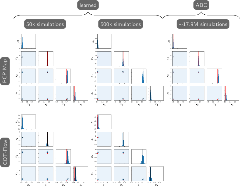
Figure 2: Posterior samples in log scale and MAP point quality comparisons between proposed approaches and ABC with ${\bf x}^{*}=(0.01,0.5,1,0.01)^{\top}$. Left: posterior samples generated by proposed approaches trained on 50k samples. Middle: posterior samples generated by proposed approaches trained on 500k samples. The red dots and bars correspond to ${\bf x}^{*}$, and the black crosses and bars correspond to the MAP point. Right: posterior samples from ABC.

For the pilot run, we use the same sample space in Table 3 except expanding the batch size space to {64, 128, 256} for PCP-Map and {32, 64, 128, 256} for COT-Flow to account for the increase in sample size. We also fixed, for PCP-Map, $w=u$. During PCP-Map’s pilot run, we perform two training epochs with 100 hyperparameter combination samples using the 50k dataset. For COT-Flow, we only perform one epoch of pilot training as it is empirically observed to be sufficient. We then use the best hyperparameter combinations to train our models on the 50k and 500k datasets to learn the posterior for the normalized parameter in the log-domain. After learning the maps, we used their inverses, the training data mean and standard deviation, and the log transformations to yield parameter samples in the original domain.

The SMC-ABC algorithm finds parameters that match the observations with respect to a selected distance function by gradually reducing a tolerance $\epsilon>0$, which leads to samples from the true posterior exactly as $\epsilon\rightarrow 0$. For our experiment, we allow $\epsilon$ to converge to $0.1$ for the first true parameter and $0.15$ for the second.

We evaluate our approaches for maximum-a-posteriori (MAP) estimation and posterior sampling. We consider a true parameter ${\bf x}^{*}=(0.01,0.5,1,0.01)^{\top}$, which was chosen to give rise to oscillatory behavior in the population time series. Given one observation ${\bf y}^{*}\sim\pi({\bf y}|{\bf x}^{*})$, we first identify the MAP point by maximizing the estimated log-likelihoods provided by our approaches. Then, we generate 2000 samples from the approximate posterior $\pi({\bf x}|{\bf y}^{*})$ using our approaches. Fig. 2 presents one and two-dimensional marginal histograms and scatter plots of the MAP point and samples, compared against 2000 samples generated by the SMC-ABC algorithm from [7]. Our approaches yield samples tightly concentrated around the MAP points that are close to the true parameter ${\bf x}^{*}$.

To provide more evidence that our learning approaches indeed solve the amortized problem, Fig. 3 shows the MAP points and approximate posterior samples generated from a new random observation ${\bf y}^{*}$ corresponding to the true parameter ${\bf x}^{*}=(0.02,0.02,0.02,0.02)^{\top}$. We observe similar concentrations of the MAP point and posterior samples around the true parameter and similar correlations learned by the generative model and ABC, for example, between the third and other parameters.

Efficiency-wise, PCP-Map and COT-Flow yield similar approximations to ABC at a fraction of the computational cost of ABC. The latter requires approximately 5 or 18 million model simulations for each conditioning observation, while the learned approaches use the same $50$ thousand simulations to amortize over the observation. These savings generally offset the hyperparameter search and training time for the proposed approaches, which is typically less than half an hour per full training run on a GPU. For some comparison, SMC-ABC took 15 days to reach $\epsilon=0.1$ for ${\bf x}^{*}=(0.01,0.5,1,0.01)^{\top}$.

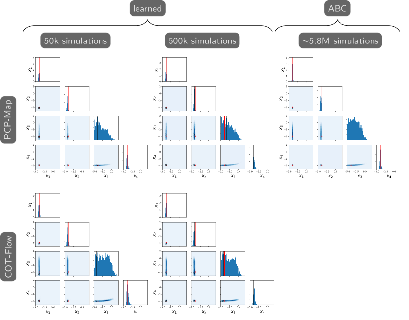
Figure 3: Posterior samples log scale and MAP point quality comparisons between proposed approaches and ABC with ${\bf x}^{*}=(0.02,0.02,0.02,0.02)^{\top}$. Left: posterior samples generated by proposed approaches trained on 50k samples. Middle: posterior samples generated by proposed approaches trained on 500k samples. The red dots and bars correspond to ${\bf x}^{*}$, and the black crosses and bars correspond to the MAP point. Right: posterior samples from ABC.

To further validate that we approximate the posterior distribution as well, Fig. 4 compares the population time series generated from approximate posterior samples given by our approaches and SMC-ABC. This corresponds to comparing the posterior predictive distributions for the states $S(t)$ given different posterior approximations for the parameters. While the simulations have inherent stochasticity, we observe that the generated posterior parameter samples from all approaches recover the expected oscillatory time series simulated from the true parameter ${\bf x}^{\ast}$, especially at earlier times.

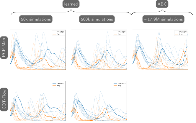
Figure 4: Posterior predictives quality comparisons between proposed approaches and ABC with ${\bf x}^{*}=(0.01,0.5,1,0.01)^{\top}$. The solid lines in each plot represent a simulated time series using ${\bf x}^{*}$. Dotted lines represent time series simulated using ten randomly selected posterior samples from the 2000. Left: posterior predictives from proposed approaches trained on 50k samples. Middle: posterior predictives from proposed approaches trained on 500k samples. Right: posterior predictives from ABC.

In the experiments above, we employed $n_{t}=32$ to generate posterior samples during testing for the COT-Flow. However, one can also decrease $n_{t}$ after training to generate samples faster without sacrificing much accuracy, as shown in Fig. 5. Thereby, one can achieve faster sampling speed using COT-Flow than using PCP-Map as demonstrated in Table 5. To establish such a comparison, we increase the $l$-BFGS tolerance when sampling using PCP-Map, which produces a similar effect on sampling accuracy than decreasing the number of time steps for COT-Flow.

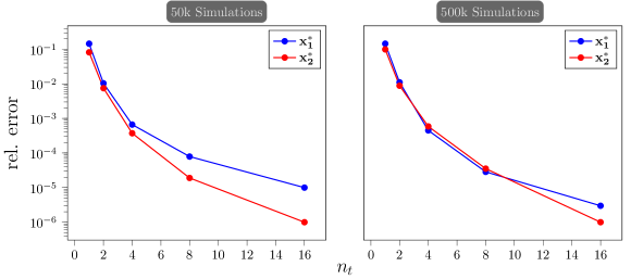
Figure 5: Relative normed errors between COT-Flow posterior samples generated with smaller $n_{t}$ values and samples generated with $n_{t}=32$. Here ${\bf x}^{*}_{1}=(0.01,0.5,1,0.01)^{\top}$ and ${\bf x}^{*}_{2}=(0.02,0.02,0.02,0.02)^{\top}$.

Table 5: Sampling efficiency comparisons between PCP-Map and COT-Flow in terms of GPU time in seconds (s). We report the mean and standard deviation over five runs, respectively.

COT-Flow Sampling (s)	PCP-Map Sampling (s)
$n_{t}$=32  0.538 $\pm$ 0.003	tol=1e-6   0.069 $\pm$ 0.004
$n_{t}$=16  0.187 $\pm$ 0.004	tol=1e-5   0.066 $\pm$ 0.004
$n_{t}$=8  0.044 $\pm$ 0.000	tol=1e-4   0.066 $\pm$ 0.004
$n_{t}$=4  0.025 $\pm$ 0.001	tol=1e-3   0.066 $\pm$ 0.004
$n_{t}$=2  0.012 $\pm$ 0.000	tol=1e-2   0.059 $\pm$ 0.001
$n_{t}$=1  0.006 $\pm$ 0.000	tol=1e-1   0.049 $\pm$ 0.004

6.3 1D Shallow Water Equations

The shallow water equations model wave propagation through shallow basins described by the depth profiles parameter, ${\bf x}\in\mathbb{R}^{100}$, which is discretized at 100 equidistant points in space. After solving the equations over a time grid with 100 cells, the resulting wave amplitudes form the 10k-dimensional raw observations. As in [40], we perform a 2D Fourier transform on the raw observations and concatenate the real and imaginary parts since the waves are periodic. We define this simulation-then-Fourier-transform process as our forward model and denote it as $\Psi({\bf x})$. Additive Gaussian noise is then introduced to the outputs of $\Psi$, which gives us the observations ${\bf y}=\Psi({\bf x})+0.25{\boldsymbol{\epsilon}}$, where ${\bf y}\in\mathbb{R}^{200\times 100}$ and ${\boldsymbol{\epsilon}}_{i,j}\sim\mathcal{N}(0,1)$. We aim to use the proposed approaches to learn the posterior $\pi({\bf x}|{\bf y})$.

We follow instructions from [40] to set up the experiment and obtain 100k samples from the joint distribution $\pi({\bf x},{\bf y})$ as the training dataset using the provided scripts. We use the prior distribution

$$\pi({\bf x})=\mathcal{N}(10\cdot\mu\mathbf{1}_{100},{\boldsymbol{\Sigma}})\;\rm\;with\;\;{\boldsymbol{\Sigma}}_{ij}=\sigma\exp\left(\frac{-(i-j)^{2}}{2\tau}\right),\;\sigma=15,\;\tau=100.$$

Using a principal component analysis (PCA), we analyze the intrinsic dimensions of ${\bf x}$ and ${\bf y}$. To ensure that the large additive noise $0.25{\boldsymbol{\epsilon}}$ does not affect our analysis, we first study another set of 100k noise-free prior predictives using the estimated covariance ${\rm Cov}({\bf Y})\approx\frac{1}{N-1}{\bf Y}^{\top}{\bf Y}$. Here, ${\bf Y}\in\mathbb{R}^{100000\times 20000}$ stores the samples row-wise in a matrix. The top 3500 modes explain around $96.5\%$ of the variance. A similar analysis on the noise-present training dataset shows that the top 3500 modes, in this case, only explain around $75.6\%$ of the variance due to the added noise. To address the rank deficiency, we construct a projection matrix ${\bf V}_{\rm proj}$ using the top 3500 eigenvectors of ${\rm Cov}({\bf Y})$ and obtain the projected observations ${\bf y}_{\rm proj}={\bf V}_{\rm proj}^{\top}{\bf y}$ from the training datasets. We then perform a similar analysis for ${\bf x}$ and discovered that the top 14 modes explained around $99.9\%$ of the variance. Hence, we obtain ${\bf x}_{\rm proj}\in\mathbb{R}^{14}$ as the projected parameters.

We then trained our approaches to learn the reduced posterior, $\pi_{\rm proj}({\bf x}_{\rm proj}|{\bf y}_{\rm proj})$. For comparisons, we trained the flow-based NPE approach to learn the same posterior exactly like did in [40]. For COT-Flow, we add a 3-layer fully connected neural network with $\tanh$ activation to embed ${\bf y}_{\rm proj}$. To pre-process the training dataset, we randomly select 5% of the dataset as the validation set and use the rest as the training set. We project both ${\bf x}$ and ${\bf y}$ and then normalize them by subtracting the empirical mean and dividing by the empirical standard deviations of the training data.

We employ the sample space presented in Table 6 for the pilot runs.

Table 6: Hyperparameter sample space for the 1D shallow water equations experiment.

Hyperparameters	PCP-Map	COT-Flow
Batch size	{64, 128, 256}	$\{2^{7},2^{8},2^{9},2^{10}\}$
Learning rate	{$10^{-2},10^{-3},10^{-4}$}	$\{10^{-2},10^{-3},10^{-4}\}$
Feature layer width, $w$	{32, 64, 128, 256, 512}	$\{512,1024\}$
Context layer width, $u$	{$u=w$}
Embedding feature width, $w_{y}$		$\{2^{5},2^{6},2^{7}\}$
Embedding output width, $w_{yout}$		$\{2^{5},2^{6},2^{7}\}$
Number of layers, $K$	{2, 3, 4, 5, 6}	{2}
Number of time steps, $n_{t}$		{8, 16}
$[\log(\alpha_{1}),\log(\alpha_{2})]$		[$\mathcal{U}(10^{2},10^{5})$, $\mathcal{U}(10^{2},10^{5})$]

For COT-Flow, we select a $w$ sample space with larger values for maximum expressiveness and allow multiple optimization steps over one batch, randomly selected from $\{8,16\}$. We then use the best hyperparameter combination based on the validation loss for the full training. For NPE, we used the sbi package [50] and the scripts provided by [40].

We first compare the accuracy of the MAP points, posterior samples, and posterior predictives across the three approaches. The MAP points are obtained using the same method as in Section 6.2. For posterior sampling, we first sample a “ground truth” ${\bf x}^{*}\sim\pi({\bf x})$ and obtain the associated ground truth reduced observation ${\bf y}^{*}_{\rm proj}={\bf V}_{\rm proj}^{\top}(\Psi({\bf x}^{*})+0.25{\boldsymbol{\epsilon}})$. Then, we use the three approaches to sample from the posterior $\pi_{\rm proj}({\bf x}_{\rm proj}|{\bf y}^{*}_{\rm proj})$. This allows us to obtain approximate samples ${\bf x}\sim\pi({\bf x}|{\bf y}^{*})$. The posterior predictives are obtained by solving the forward model for the generated parameters. Through Fig. 6, we observe that the MAP points, posterior samples, and predictives produced by PCP-Map and COT-Flow are more concentrated around the ground truth than those produced by NPE.

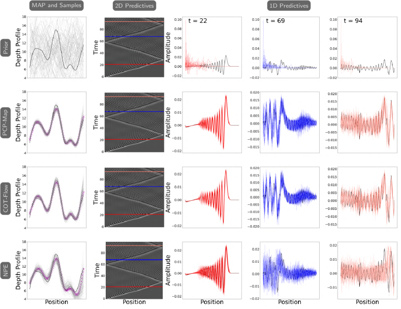
Figure 6: Prior, MAP point, posterior samples, and predictives quality comparisons between PCP-Map, COT-Flow, and NPE. Each Row: left: prior (first row) or posterior samples in gray and ${\bf x}^{*}$ in black. middle: 2D image of the wave amplitudes simulated using ${\bf x}^{*}$ (first row) or posterior samples for 100 time grids. right: wave amplitudes simulated using 50 prior (first row) or posterior samples at t = 22, 69, 94. Here ${\bf y}^{*}$ is plotted in black.

We perform the simulation-based calibration (SBC) analysis described in  [40, App. D.2] to further assess the three approaches’ accuracy; see Fig. 7. We can see that, while they are all well calibrated, the cumulative density functions of the rank statistics produced by PCP-Map align almost perfectly with the CDF of a uniform distribution besides a few outliers.

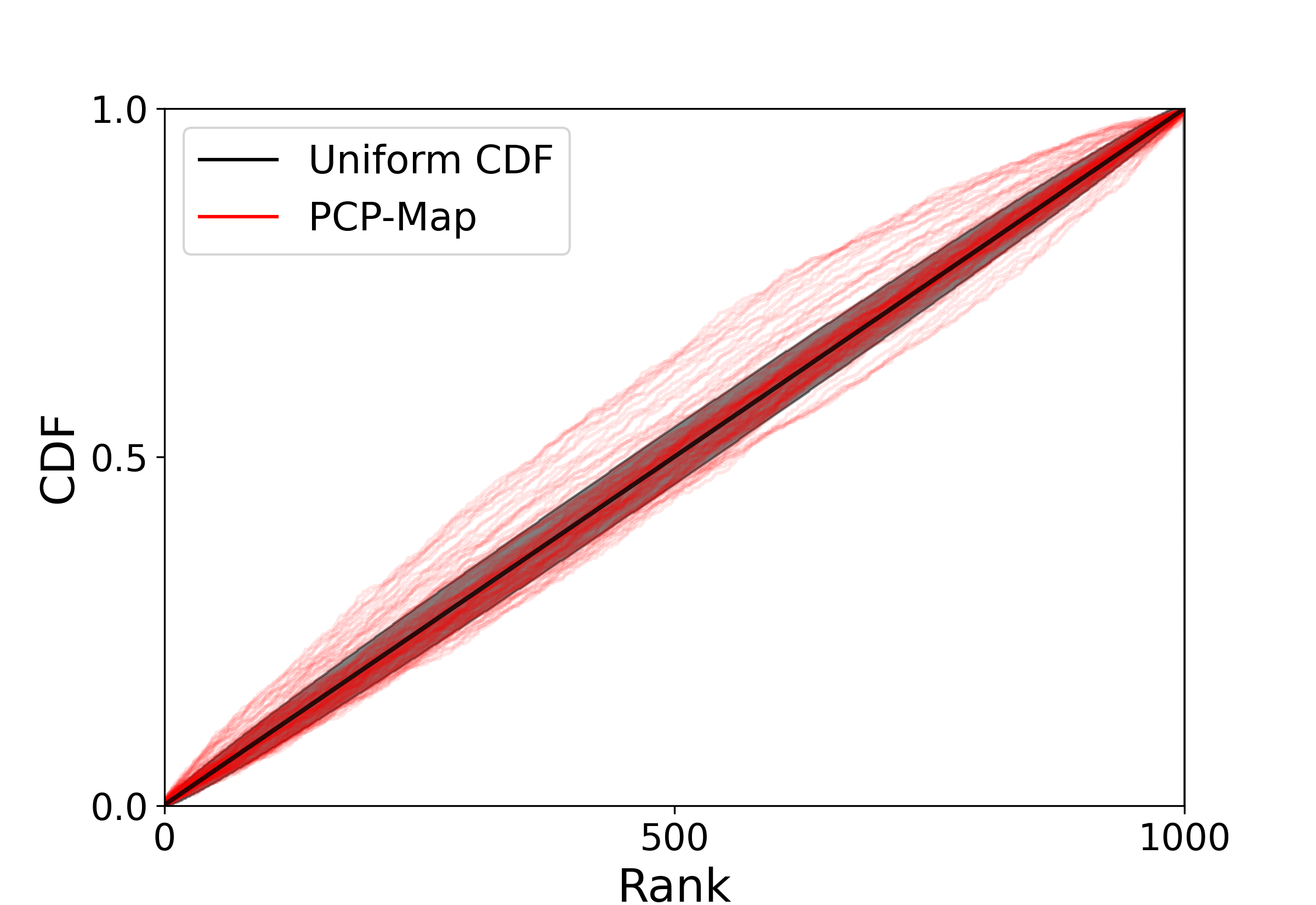
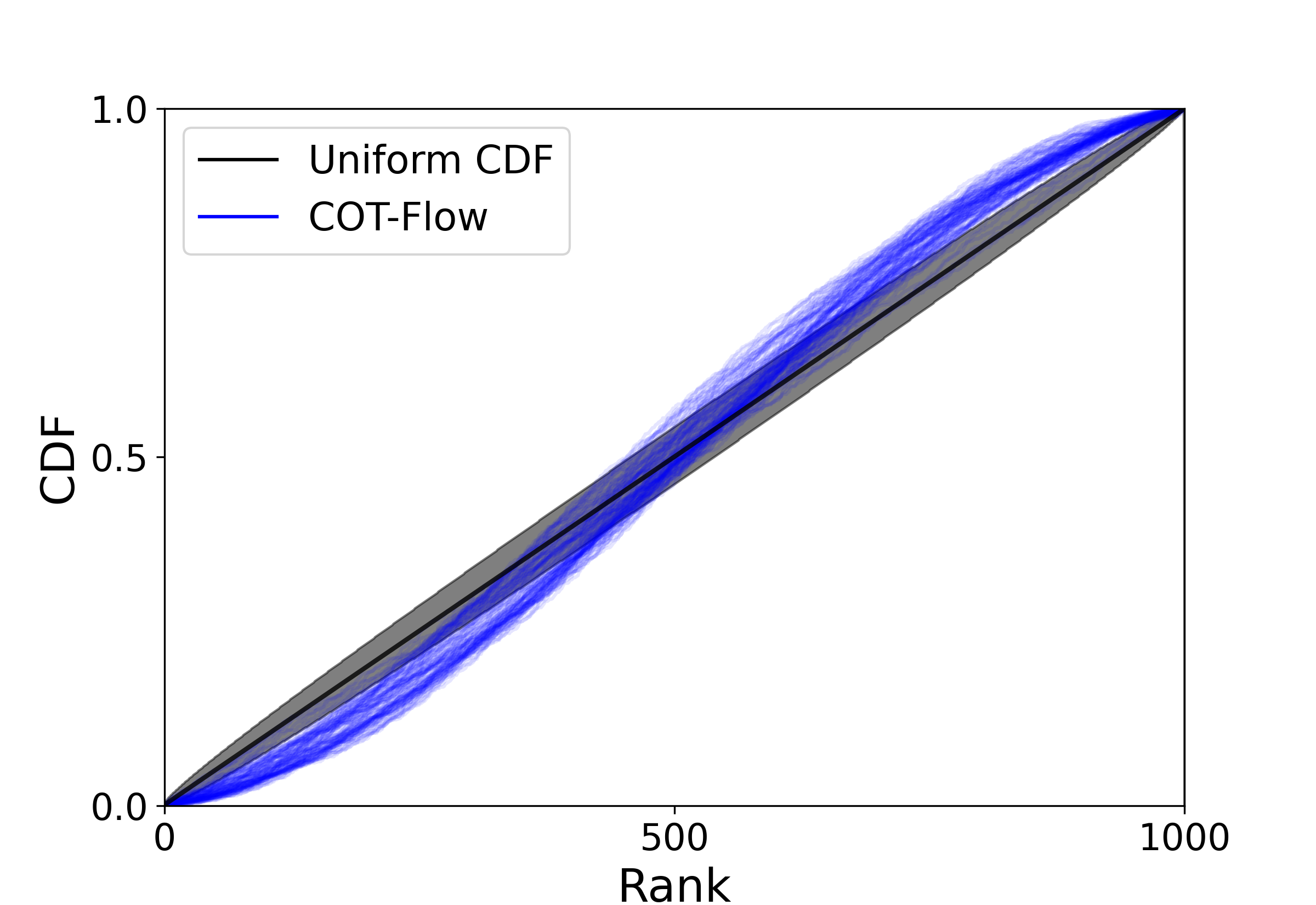
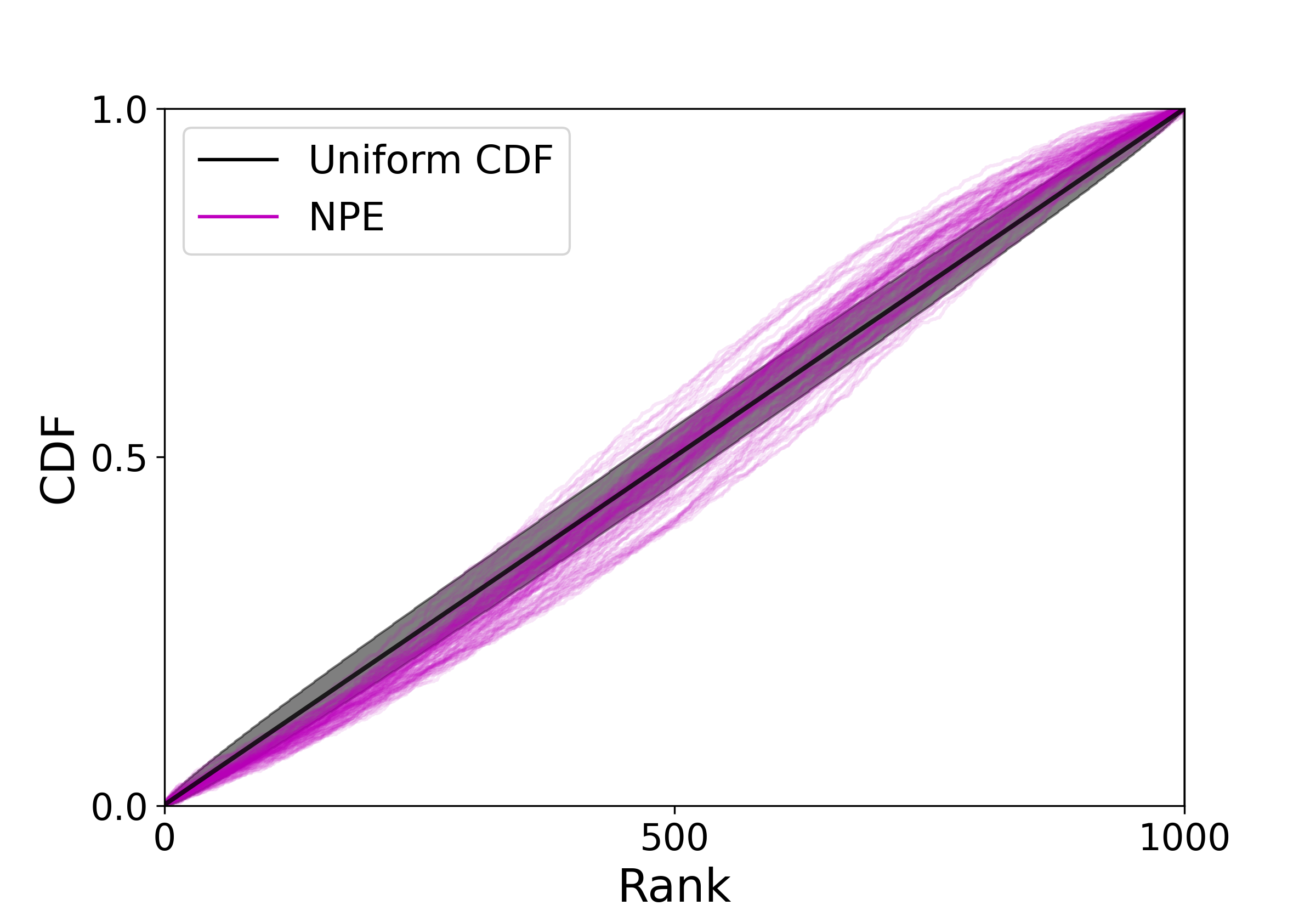
Figure 7: SBC Analysis for PCP-Map, COT-Flow and NPE. Each colored line represents the empirical cumulative density function (CDF) of the SBC rank associated with one posterior sample dimension.

Finally, we analyze the three approaches’ efficiency in terms of the number of forward model evaluations. We train the models using the best hyperparameter combinations from the pilot run on two extra datasets with 50k and 20k samples. We compare the posterior samples’ mean and standard deviation against ${\bf x}^{*}$ across three approaches trained on the 100k, 50k, and 20k sized datasets as presented in Fig. 8. We see that PCP-Map and COT-Flow can generate posterior samples centered more closely around the ground truth than NPE using only 50k training samples, which translates to higher computational efficiency since fewer forward model evaluations are required.

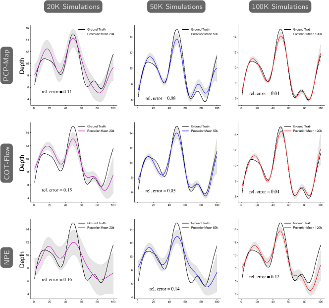
Figure 8: Posterior sample quality comparisons between PCP-Map, COT-Flow, and NPE trained using 20k, 50k, and 100k samples. We report the relative normed error between the posterior sample mean (over 100 samples) and the ground truth parameter. The gray bands represent regions within one standard deviation of the means.

6.4 Comparing PCP-Map to amortized CP Flow

We conduct this comparative experiment using the shallow water equations problem for its high dimensionality. We include the more challenging task of learning $\pi({\bf x}|{\bf y}_{\rm proj})$, obtained without projecting the parameter, to test the two approaches most effectively. We followed [20] and its associated GitHub repository as closely as possible to implement the amortized CP-Flow. To ensure as fair of a comparison as possible, we used the hyperparameter combination from the amortized CP-Flow pilot run for learning $\pi({\bf x}|{\bf y}_{\rm proj})$ and the combination from the PCP-Map pilot run for learning $\pi_{\rm proj}({\bf x}_{\rm proj}|{\bf y}_{\rm proj})$. Note that for learning $\pi({\bf x}|{\bf y}_{\rm proj})$, we limited the learning rate to $\{0.0001\}$ for which we observed reasonable convergence.

In the experiment, we observed that amortized CP-Flow’s Hessian vector product function gave NaNs consistently when computing the stochastic log-determinant estimation. Thus, we resorted to exact computation for the pilot and training runs. PCP-Map circumvents this as it uses exact log-determinant computations. Each model was trained five times to capture possible variance.

For comparison, we use the exact mean negative log-likelihood as the metric for accuracy and GPU time as the metric for computational cost. We only record the time for loss function evaluations and optimizer steps for both approaches. The comparative results are presented in Table 7. We see that PCP-Map and amortized CP-Flow reach similar training and validation accuracy. However, PCP-Map takes roughly 7 and 3 times less GPU time, respectively, on average, to achieve that accuracy than amortized CP-Flow. Possible reasons for the increased efficiency of PCP-Map’s are its use of ReLU non-negative projection, vectorized Hessian computation, removal of activation normalization, and gradient clipping.

Table 7: Computational cost comparisons between amortized CP-Flow and PCP-Map in terms of GPU time in seconds (s). We report the mean and standard deviation of the training and validation mean NLL, the mean and standard deviation of the GPU times over five training runs, and the number of parameters in million(M), respectively.

	$\pi({\bf x}|{\bf y}_{\rm proj})$		$\pi_{\rm proj}({\bf x}_{\rm proj}|{\bf y}_{\rm proj})$
Approach	PCP-Map	CP-Flow	PCP-Map	CP-Flow
Number of Parameters	$\sim$8.9M	$\sim$5.7M	$\sim$2.5M	$\sim$1.4M
Training Mean NLL	$-540.3\pm 4.5$	$-534.2\pm 9.1$	$-5.8\pm 0.6$	$-6.6\pm 0.3$
Validation Mean NLL	$-519.0\pm 4.1$	$-506.4\pm 5.1$	$8.5\pm 0.1$	$6.1\pm 0.2$
Training(s)	6652.2$\pm$1030.3	47207.4$\pm$7221.0	706.9$\pm$61.0	1989.4$\pm$10.5
Validation(s)	108.5$\pm$17.1	232.1$\pm$35.5	6.6$\pm$0.6	10.3$\pm$0.1
Total(s)	6760.7$\pm$1047.4	47439.5$\pm$7256.4	713.5$\pm$61.5	1999.7$\pm$10.5

7 Discussion

We present two measure transport approaches, PCP-Map and COT-Flow, that learn conditional distributions by approximately solving the static and dynamic conditional optimal transport problems, respectively. Specifically, penalizing transport costs in the learning problem provides unique optimal transport maps, known as the conditional Brenier map, between the target conditional distribution and the reference. Furthermore, for PCP-Map, minimizing the quadratic transport costs motivate us to exploit the structure of the Brenier map by constraining the search to monotone maps given as the gradient of convex potentials. Similarly, for COT flow this choice leads to a conservative vector field, which we enforce by design.

Our comparison to the SMC-ABC approach for the stochastic Lotka-Volterra problem shows common trade-offs when selecting conditional sampling approaches. Advantages of the ABC approach include its strong theoretical guarantees and well-known guidelines for choosing the involved hyper-parameters (annealing, burn-in, number of samples to skip to reduce correlation, etc.). The disadvantages are that ABC typically requires a large number of likelihood evaluations to produce (approximately) i.i.d. samples and produce low-variance estimators in high-dimensional parameter spaces; the computation is difficult to parallelize in the sequential Monte Carlo setting, and the sampling process is not amortized over the conditioning variable ${\bf y}^{*}$, i.e., it needs to be recomputed whenever ${\bf y}^{*}$ changes.

Comparisons to the flow-based NPE method for the high-dimensional 1D shallow water equations problem illustrate the superior numerical accuracy achieved by our approaches. In terms of numerical efficiency, the PCP-Map approach, while providing a working computational scheme to the static COT problem, achieves significantly faster convergence than the amortized CP-Flow approach.

Learning posterior distributions using our techniques or similar measure transport approaches is attractive for real-world applications where samples from the joint distributions are available (or can be generated efficiently), but evaluating the prior density or the likelihood model is intractable. Common examples where a non-intrusive approach for conditional sampling can be fruitful include inverse problems where the predictive model involves stochastic differential equations (as in Section 6.2) or legacy code and imaging problems where only prior samples are available.

Given the empirical nature of our study, we paid particular attention to the setup and reproducibility of our numerical experiments. To show the robustness of our approaches to hyperparameters and to provide guidelines for hyperparameter selection in future experiments, we report the results of a simple two-step heuristic that randomly samples hyperparameters and identifies the most promising configurations after a small number of training steps. We stress that the same search space of hyperparameters is used across all numerical experiments.

The results of the shallow water dataset Section 6.3 indicate that both methods can learn high-dimensional COT maps. Here, the number of effective parameters in the dataset was $n=14$, and the number of effective measurements was $m=3500$. Particularly worth noting is that PCP-Map, on average, converges in around 715 seconds on this challenging high-dimensional problem.

Since both approaches perform similarly in our numerical experiments, we want to comment on some distinguishing factors. One advantage of the PCP-Map approach is that it only depends on three hyperparameters (feature width, context width, and network depth), and we observed consistent performance for most choices. This feature is particularly attractive when experimenting with new problems. The limitation is that a carefully designed network architecture needs to be imposed to guarantee partial convexity of the potential. On the other hand, the value function (i.e., the velocity field) in COT-Flow can be designed almost arbitrarily. Thus, the latter approach may be beneficial when new data types and their invariances need to be modeled, e.g., permutation invariances or symmetries, that might conflict with the network architecture required by the direct transport map. Both approaches also differ in terms of their numerical implementation. Training the PCP-Map via backpropagation is relatively straightforward, but sampling requires solving a convex program, which can be more expensive than integrating the ODE defined by the COT-Flow approach, especially when that model is trained well, and the velocity is constant along trajectories. Training the COT-Flow model, however, is more involved due to the ODE constraints.

Although our numerical evidence supports the effectiveness of our methods, important remaining limitations of our approaches include the absence of theoretical guarantees for sample efficiency and optimization. In particular, statistical complexity and approximation theoretic analysis for approximating COT maps using PCP-Map or COT-Flow in a conditional sampling context will be beneficial. We also point out that it can be difficult to quantify the produced samples’ accuracy without a benchmark method.

References

- [1] L. Ambrogioni, U. Güçlü, M. A. J. van Gerven, and E. Maris, The kernel mixture network: A nonparametric method for conditional density estimation of continuous random variables, 2017, https://arxiv.org/abs/1705.07111.
- [2] B. Amos, L. Xu, and J. Z. Kolter, Input convex neural networks, in International Conference on Machine Learning, 2017, pp. 146–155.
- [3] R. Baptista, B. Hosseini, N. B. Kovachki, and Y. Marzouk, Conditional sampling with monotone gans: from generative models to likelihood-free inference, 2023, https://arxiv.org/abs/2006.06755.
- [4] R. Baptista, Y. Marzouk, and O. Zahm, On the representation and learning of monotone triangular transport maps, 2022, https://arxiv.org/abs/2009.10303.
- [5] G. Batzolis, J. Stanczuk, C.-B. Schönlieb, and C. Etmann, Conditional image generation with score-based diffusion models, arXiv preprint arXiv:2111.13606, (2021).
- [6] C. M. Bishop, Mixture density networks, Technical Report NCRG/94/004, Aston University, Department of Computer Science and Applied Mathematics, 1994., (1994).
- [7] F. V. Bonassi and M. West, Sequential monte carlo with adaptive weights for approximate bayesian computation, Bayesian Analysis, 10 (2015), pp. 171–187.
- [8] Y. Brenier, Polar factorization and monotone rearrangement of vector-valued functions, Communications on pure and applied mathematics, 44 (1991), pp. 375–417.
- [9] C. Bunne, A. Krause, and M. Cuturi, Supervised training of conditional monge maps, in Advances in Neural Information Processing Systems, S. Koyejo, S. Mohamed, A. Agarwal, D. Belgrave, K. Cho, and A. Oh, eds., vol. 35, Curran Associates, Inc., 2022, pp. 6859–6872.
- [10] G. Carlier, V. Chernozhukov, and A. Galichon, Vector quantile regression: An optimal transport approach, Annals of Statistics, 44 (2014), pp. 1165–1192.
- [11] R. T. Q. Chen, J. Behrmann, D. K. Duvenaud, and J.-H. Jacobsen, Residual flows for invertible generative modeling, in Advances in Neural Information Processing Systems, vol. 32, Curran Associates, Inc., 2019.
- [12] K. Cranmer, J. Brehmer, and G. Louppe, The frontier of simulation-based inference, Proceedings of the National Academy of Sciences, 117 (2020), pp. 30055–30062.
- [13] N. De Cao, W. Aziz, and I. Titov, Block neural autoregressive flow, in Proceedings of The 35th Uncertainty in Artificial Intelligence Conference, vol. 115 of Proceedings of Machine Learning Research, PMLR, 22–25 Jul 2020, pp. 1263–1273.
- [14] L. Dinh, J. Sohl-Dickstein, and S. Bengio, Density estimation using real NVP, in International Conference on Learning Representations, 2017.
- [15] C. Durkan, A. Bekasov, I. Murray, and G. Papamakarios, Neural spline flows, in Advances in Neural Information Processing Systems, vol. 32, Curran Associates, Inc., 2019.
- [16] A. Figalli and F. Glaudo, An Invitation to Optimal Transport, Wasserstein Distances, and Gradient Flows, EMS Press, 2021.
- [17] C. Finlay, J.-H. Jacobsen, L. Nurbekyan, and A. Oberman, How to train your neural ODE: the world of Jacobian and kinetic regularization, in Proceedings of the 37th International Conference on Machine Learning, vol. 119 of Proceedings of Machine Learning Research, PMLR, 13–18 Jul 2020, pp. 3154–3164.
- [18] M. Grant, S. Boyd, and Y. Ye, Disciplined Convex Programming, Springer US, Boston, MA, 01 2006, pp. 155–210, https://doi.org/10.1007/0-387-30528-9_7.
- [19] W. Grathwohl, R. T. Chen, J. Betterncourt, I. Sutskever, and D. Duvenaud, FFJORD: Free-form continuous dynamics for scalable reversible generative models, in International Conference on Learning Representations (ICLR), 2019.
- [20] C.-W. Huang, R. T. Q. Chen, C. Tsirigotis, and A. Courville, Convex potential flows: Universal probability distributions with optimal transport and convex optimization, in International Conference on Learning Representations, 2021.
- [21] C.-W. Huang, D. Krueger, A. Lacoste, and A. Courville, Neural autoregressive flows, in Proceedings of the 35th International Conference on Machine Learning, vol. 80 of Proceedings of Machine Learning Research, PMLR, 10–15 Jul 2018, pp. 2078–2087.
- [22] N. J. Irons, M. Scetbon, S. Pal, and Z. Harchaoui, Triangular flows for generative modeling: Statistical consistency, smoothness classes, and fast rates, in International Conference on Artificial Intelligence and Statistics, 2021.
- [23] J. Kim and Y. Kim, Parameterized convex universal approximators for decision-making problems, IEEE Transactions on Neural Networks and Learning Systems, (2022), pp. 1–12, https://doi.org/10.1109/TNNLS.2022.3190198.
- [24] D. P. Kingma and J. Ba, Adam: A method for stochastic optimization, arXiv preprint arXiv:1412.6980, (2014).
- [25] D. P. Kingma and P. Dhariwal, Glow: Generative flow with invertible 1x1 convolutions, in Advances in Neural Information Processing Systems, vol. 31, 2018.
- [26] D. P. Kingma, T. Salimans, R. Jozefowicz, X. Chen, I. Sutskever, and M. Welling, Improved variational inference with inverse autoregressive flow, in Advances in Neural Information Processing Systems, vol. 29, 2016, pp. 4743–4751.
- [27] I. Kobyzev, S. J. Prince, and M. A. Brubaker, Normalizing flows: An introduction and review of current methods, IEEE Transactions on Pattern Analysis and Machine Intelligence, 43 (2021), pp. 3964–3979, https://doi.org/10.1109/tpami.2020.2992934, https://doi.org/10.1109%2Ftpami.2020.2992934.
- [28] J.-M. Lasry and P.-L. Lions, Mean field games, Japanese Journal of Mathematics, 2 (2007), pp. 229–260, https://doi.org/10.1007/s11537-007-0657-8.
- [29] M. Lichman et al., UCI machine learning repository, 2013.
- [30] S. Liu, X. Zhou, Y. Jiao, and J. Huang, Wasserstein generative learning of conditional distribution, ArXiv, abs/2112.10039 (2021).
- [31] Y. Lu and B. Huang, Structured output learning with conditional generative flows, Proceedings of the AAAI Conference on Artificial Intelligence, 34 (2020), pp. 5005–5012, https://doi.org/10.1609/aaai.v34i04.5940, https://ojs.aaai.org/index.php/AAAI/article/view/5940.
- [32] A. Makkuva, A. Taghvaei, S. Oh, and J. Lee, Optimal transport mapping via input convex neural networks, in International Conference on Machine Learning, PMLR, 2020, pp. 6672–6681.
- [33] Y. Marzouk, T. Moselhy, M. Parno, and A. Spantini, Sampling via measure transport: An introduction, Handbook of uncertainty quantification, 1 (2016), p. 2.
- [34] M. Mirza and S. Osindero, Conditional generative adversarial nets, arXiv:1411.1784, (2014).
- [35] S. N. Negahban, P. Ravikumar, M. J. Wainwright, and B. Yu, A Unified Framework for High-Dimensional Analysis of -Estimators with Decomposable Regularizers, Statistical Science, 27 (2012), pp. 538 – 557, https://doi.org/10.1214/12-STS400, https://doi.org/10.1214/12-STS400.
- [36] D. Onken, S. Wu Fung, X. Li, and L. Ruthotto, OT-Flow: Fast and accurate continuous normalizing flows via optimal transport, Proceedings of the AAAI Conference on Artificial Intelligence, 35, https://par.nsf.gov/biblio/10232664.
- [37] G. Papamakarios and I. Murray, Fast -free inference of simulation models with Bayesian conditional density estimation, in Advances in Neural Information Processing Systems, vol. 29, Curran Associates, Inc., 2016.
- [38] G. Papamakarios, E. Nalisnick, D. J. Rezende, S. Mohamed, and B. Lakshminarayanan, Normalizing flows for probabilistic modeling and inference, The Journal of Machine Learning Research, 22 (2021), pp. 2617–2680.
- [39] G. Papamakarios, T. Pavlakou, and I. Murray, Masked autoregressive flow for density estimation, in Advances in Neural Information Processing Systems, vol. 30, Curran Associates, Inc., 2017.
- [40] P. Ramesh, J.-M. Lueckmann, J. Boelts, Á. Tejero-Cantero, D. S. Greenberg, P. J. Gonçalves, and J. H. Macke, GATSBI: Generative Adversarial Training for Simulation-Based Inference, in Proceedings of the 10th International Conference on Learning Representations (ICLR 2022), Online, 2022.
- [41] J. Rothfuss, F. Ferreira, S. Walther, and M. Ulrich, Conditional density estimation with neural networks: Best practices and benchmarks, ArXiv, abs/1903.00954 (2019).
- [42] L. Ruthotto and E. Haber, An Introduction to Deep Generative Modeling, GAMM Mitteilungen, cs.LG (2021).
- [43] L. Ruthotto, S. J. Osher, W. Li, L. Nurbekyan, and S. W. Fung, A machine learning framework for solving high-dimensional mean field game and mean field control problems, Proceedings of the National Academy of Sciences, 117 (2020), pp. 9183 – 9193, https://doi.org/10.1073/pnas.1922204117/-/dcsupplemental.
- [44] M. Shiga, V. Tangkaratt, and M. Sugiyama, Direct conditional probability density estimation with sparse feature selection, Machine Learning, 100 (2015), pp. 161 – 182.
- [45] K. Sohn, H. Lee, and X. Yan, Learning structured output representation using deep conditional generative models, in Advances in Neural Information Processing Systems, vol. 28, Curran Associates, Inc., 2015.
- [46] Y. Song, J. Sohl-Dickstein, D. P. Kingma, A. Kumar, S. Ermon, and B. Poole, Score-based generative modeling through stochastic differential equations, in International Conference on Learning Representations, 2021.
- [47] A. Spantini, R. Baptista, and Y. Marzouk, Coupling techniques for nonlinear ensemble filtering, SIAM Review, 64 (2022), pp. 921–953, https://doi.org/10.1137/20M1312204.
- [48] K. Tang, X. Wan, and Q. Liao, Deep density estimation via invertible block-triangular mapping, Theoretical and Applied Mechanics Letters, 10 (2020), pp. 143–148.
- [49] Y. Tashiro, J. Song, Y. Song, and S. Ermon, CSDI: Conditional score-based diffusion models for probabilistic time series imputation, in Neural Information Processing Systems, 2021.
- [50] A. Tejero-Cantero, J. Boelts, M. Deistler, J.-M. Lueckmann, C. Durkan, P. J. Gonçalves, D. S. Greenberg, and J. H. Macke, sbi: A toolkit for simulation-based inference, Journal of Open Source Software, 5 (2020), p. 2505.
- [51] A. Tong, N. Malkin, G. Huguet, Y. Zhang, J. Rector-Brooks, K. FATRAS, G. Wolf, and Y. Bengio, Improving and generalizing flow-based generative models with minibatch optimal transport, in ICML Workshop on New Frontiers in Learning, Control, and Dynamical Systems, 2023.
- [52] C. Villani et al., Optimal transport: old and new, vol. 338, Springer, 2009.
- [53] A. Wehenkel and G. Louppe, Unconstrained monotonic neural networks, in Advances in Neural Information Processing Systems, vol. 32, 2019.
- [54] J. Whang, E. Lindgren, and A. Dimakis, Composing normalizing flows for inverse problems, in International Conference on Machine Learning, PMLR, 2021, pp. 11158–11169.
- [55] D. J. Wilkinson, Stochastic modelling for systems biology, CRC press, 2018.
- [56] L. Yang and G. E. Karniadakis, Potential flow generator with optimal transport regularity for generative models, IEEE Transactions on Neural Networks and Learning Systems, 33 (2022), pp. 528–538, https://doi.org/10.1109/TNNLS.2020.3028042.
- [57] B. J. Zhang and M. A. Katsoulakis, A mean-field games laboratory for generative modeling, arXiv, (2023), https://arxiv.org/abs/2304.13534.
- [58] L. Zhang, W. E, and L. Wang, Monge-Ampère flow for generative modeling, 2018, https://arxiv.org/abs/1809.10188.