Inchworm quasi Monte Carlo for quantum impurities

Abstract

The inchworm expansion is a promising approach to solving strongly correlated quantum impurity models due to its reduction of the sign problem in real and imaginary time. However, inchworm Monte Carlo is computationally expensive, converging as $1/\sqrt{N}$ where $N$ is the number of samples. We show that the imaginary time integration is amenable to quasi Monte Carlo, with enhanced $1/N$ convergence, by mapping the Sobol low-discrepancy sequence from the hypercube to the simplex with the so-called Root transform. This extends the applicability of the inchworm method to, e.g., multi-orbital Anderson impurity models with off-diagonal hybridization, relevant for materials simulation, where continuous time hybridization expansion Monte Carlo has a severe sign problem.

Quantum impurity models are key for describing the physics of low dimensional quantum systems such as quantum dots [1], molecular junctions [2], and cold atom systems [3] which can exhibit quantum many-body effects like the Coulomb blockade [4] and Kondo screening [5, 6]. Quantum impurity models are also central for the ab-initio simulation of correlated quantum materials where they appear as auxiliary problems within dynamical mean-field theory [7] and its extensions [8, 9, 10, 11]. Therefore, efficient simulation of quantum impurity models is of paramount importance to improving our understanding of quantum dots, correlated materials and their emergent collective phenomena, like anomalous superconductivity [12], metal–insulator transitions [13], and magnetic order [14, 15].

In thermal equilibrium, continuous time quantum Monte Carlo [16, 17, 18] provides numerically exact solutions to a wide range of quantum impurity problems, e.g. multi channel quantum dots connected to separate reservoirs and correlated materials with high symmetry. For multi-channel and multi-orbital impurities, the continuous time hybridization expansion algorithm (CTHYB) [19, 20, 21] has been particularly important for progress in the field. However, for intermixed reservoirs, low crystal symmetry, and materials with relativistic mixing of spin and orbital momentum, the majority of continuous time quantum Monte Carlo algorithms suffer from a sign problem [18].

One notable exception is inchworm quantum Monte Carlo [22, 23], where causality is exploited to reorder the diagram summation. The reordering has been shown to give sub-exponential decay of the average sign in real time [22], as well as a drastic improvement in the sign for low symmetry equilibrium problems, where CTHYB suffers from a dire sign problem [23]. However, the attainable accuracy is limited by the $1/\sqrt{N}$ convergence of the integration with the number of Monte Carlo steps $N$. Additionally, the order-by-order Monte Carlo integrals are normalized by overlaps with low order diagrams, which becomes difficult at lower temperatures [24].

In this letter, we show that by using quasi Monte Carlo integration [25, 26, 27] in imaginary time the convergence rate can be improved from $1/\sqrt{N}$ to $1/N$, greatly increasing the efficiency of the algorithm (see Fig. 1). Additionally, since quasi Monte Carlo is a direct integration technique there is no need for order-by-order normalization. We benchmark our quasi Monte Carlo inchworm algorithm on several impurity models computing both the local many-body density matrix as well as single- and two-particle response functions.

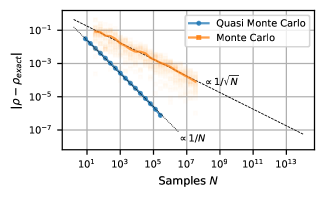
Figure 1: Absolute error $|\rho-\rho_{exact}|$ in the many body density matrix $\rho$ as a function of the number of samples $N$ for the proposed inchworm quasi Monte Carlo algorithm (blue circles) with $1/N$ scaling (dotted line) compared to the Monte Carlo based continuous time hybridization expansion [19, 20, 21, 28, 29] (orange squares) with $1/\sqrt{N}$ scaling (dashed line).

Inchworm algorithm. In its original formulation, the inchworm quantum Monte Carlo method is a stochastic strong coupling technique for solving general quantum impurity models [22]. The algorithm relies on the causality property of the pseudo-particle propagator $P(\tau)$ [30], which is computed step by step starting at $\tau_{i}=0$ and ending at $\tau_{f}=\beta$ where $\beta$ is the inverse temperature. At each step, a short (compared to $\beta$) new segment $[\tau_{w};\tau_{f}]$ is attached to the previously computed segment $[0;\tau_{w}]$, see Fig. 2. Once $P(\tau)$ has been determined, the single-particle Green’s functions $G_{\alpha\beta}(\tau)=-\langle\mathcal{T}c_{\alpha}(\tau)c_{\beta}^{\dagger}(0)\rangle$ is computed as a sum over another set of diagrams [24].

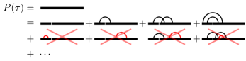
Figure 2: Modified inchworm expansion for the pseudo-particle propagator $P(\tau)$ with bold propagators on both sides of $\tau_{w}$.

Quasi Monte Carlo integration on the simplex. For each step of the inchworm algorithm all possible inchworm proper [22, 24] diagrams have to be integrated over the internal imaginary times. The internal times $\tau_{j}$ are ordered, i.e. $\tau_{f}\geq\tau_{1}\geq\tau_{2}\geq\ldots\geq\tau_{d}\geq 0$, and the integration domain is a $d$-dimensional simplex. However, the low-discrepancy sequences used for quasi Monte Carlo integration, like the Sobol sequence [31] used in our calculations, are commonly defined in the $d$-dimensional hypercube $\vec{x}\in[0,1]^{d}$. Hence, a transformation that maps the $d$-dimensional hypercube to the $d$-dimensional simplex, while preserving the low discrepancy property of the transformed sequence is required. We adopt the Root transformation [32]

$$\tau_{1}=\tau_{f}x_{1}^{1/d},\quad\tau_{2}=\tau_{1}x_{2}^{1/(d-1)},\,\ldots,\quad\tau_{d}=\tau_{d-1}x_{d}\,,$$ (1)

which is continuous, has a constant Jacobian $\tau_{f}^{d}/d!$, and with linear complexity in the dimension $d$ is computationally feasible in high dimensions. Figure 3 shows the distribution of points in the two- and three-dimensional $\tau$-simplex obtained by Root-transforming the first 1024 points of the Sobol sequence.

Unlike an earlier proposed transformation based on an exponential model function [33], the Root transformation has no free adjustable parameters and does not discard any points from the input low-discrepancy sequence. The latter feature has recently been shown to be of crucial importance [34], as skipping even one point spoils the digital net property of the sequence and can worsen the convergence rate. Furthermore, numerical experiments with individual low order inchworm diagrams showed that it outperforms the alternatives from [32, 33] in terms of the relative error scaling with the number of taken samples.

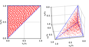
Figure 3: Sobol sequences with 1024 points mapped from the hypercube to the simplex in two (left panel) and three (right panel) dimensions using the Root transform [32] in Eq. (1).

Inchworm Quasi Monte Carlo. Our implementation of the inchworm algorithm does not rely on any form of importance sampling. Instead, the imaginary time integrals are computed using quasi Monte Carlo integration [25, 26, 27]. The remaining discrete parameters labeling various contributions to the strong coupling series – such as expansion order, spin projections and orbital indices – are explicitly summed over. This approach is straightforward, well controlled yet fast enough for the moderate expansion orders $n_{max}$ explored here ($n_{max}\lesssim 7$).

At a given inchworm step defined by ($\tau_{w},\tau_{f}$), the accumulation of the bold pseudo-particle propagators proceeds as follows. For each expansion order $n$ up to a fixed $n_{\mathrm{max}}$, a list of $n!$ diagram topologies is generated. A topology is a partition of the tuple $\{1,\ldots,2n\}$ into pairs. Diagrammatically, is can be thought of as a set of $n$ undirected hybridization lines connecting pairs of vertices located at positions $\{1,\ldots,2n\}$ on the segment $[0;\tau_{f}]$. If each hybridization line is connected by crossings to a line that overarches $\tau_{w}$, the corresponding topology is inchworm proper [22, 24], c.f. Fig. 2. Note, this differs slightly from previous definitions because we choose to use the bold rather than bare propagator between $\tau_{w}$ and $\tau_{f}$. This adjustment marginally reduces the number of diagrams appearing in the expansion. All the proper topologies are then transformed into diagrams by replacing the paired vertices with all possible pairs of operators $c_{\alpha}$ and $c_{\beta}^{\dagger}$ (swapping $c$ and $c^{\dagger}$ within a pair results in a different diagram). Finally, a sum of all contributing diagrams of order $n$ is integrated over the imaginary time domain by evaluating it at the first $N=2^{m}$ Root-transformed points of a $2n$-dimensional Sobol sequence. The power-of-two sample size restriction to $N$ is essential to preserve the digital net property of the Sobol sequence; Using other sample sizes, e.g. $10^{m}$, serverely degrades accuracy [34].

As is known in the context of hybridization expansion methods [21], a significant fraction of diagrams stemming from a retained topology do not actually contribute due to symmetry considerations. We employ the autopartition algorithm [35] to reveal invariant subspaces of the atomic Hamiltonian and to unitarily transform the matrix-valued bare pseudo-particle propagator $P_{0}(\tau)$ into a block-diagonal form. The choice of the invariant subspaces accounts for any potential symmetry breaking caused by a non-diagonal hybridization function. This way, we ensure that the subspace partition is not too refined, and that boldified propagator $P(\tau)$ possesses the same block-diagonal form.

A Julia package implementing the proposed method is publicly available at [36]. It relies on the Keldysh.jl framework [37] for handling pseudo-particle propagators and Green’s functions, and on the KeldyshED.jl package [38] for solving the atomic problem and construction of the bare atomic propagators $P_{0}(\tau)$.

Benchmarks.

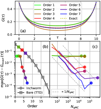
Figure 4: Panel (a): Imaginary time single-particle Green’s function $G(\tau)$ from inchworm quasi Monte Carlo at expansion orders $n_{max}=1$ to 7 (solid lines) compared to the exact solution (dashed line) at $\beta=10$. Panel (b): Expansion order convergence of the error $\max_{\tau}|G(\tau)-G_{exact}(\tau)|$ (circles) compared to the bare TTD expansion error (at $\tau=\beta/2$) (squares) [39]. Panel (c): Convergence with respect to quasi Monte Carlo samples $N_{\text{qMC}}$ at fixed order.

The theory of quasi Monte Carlo integration [25, 26, 27] only promises $1/N$ convergence for well behaved integrands and a crossover to the generic Monte Carlo scaling $1/\sqrt{N}$ for ill-behaved integrands. Hence, it is important to perform a direct investigation of the convergence rate when applying quasi Monte Carlo to a new class of problems.

To establish the convergence rate we study an impurity problem with a known analytical solution, namely a single fermionic state hybridized with a semi-infinite chain with nearest neighbor hopping. Since this system is non-interacting it can be solved exactly and it is also a worst case scenario impurity model for the strong coupling expansion, far from the atomic limit. The action $\mathcal{S}$ of the impurity model has the form

$$\mathcal{S}[c,c^{\dagger}]=-\!\!\int_{0}^{\beta}\!\!\!d\tau d\tau^{\prime}\,c^{\dagger}(\tau)\left[-\delta(\tau\!-\!\tau^{\prime})\partial_{\tau}-\Delta(\tau\!-\!\tau^{\prime})\right]c(\tau^{\prime})\,,$$ (2)

where $c^{\dagger}$ and $c$ are creation and annihilation operators of the spinless fermion, and $\Delta(\tau)$ is the hybridization function of the semi-infinite chain. It is derived from a semi-circular density of states with bandwidth $W$ coupled to the impurity with the hybridization strength $V$.

The convergence rate of the many-body density matrix $\rho=P(\beta)$ as a function of number of samples $N$ per inchworm step, in Fig. 1, is monotonic with a clear $1/N$ scaling. The difference compared to standard partition function Monte Carlo and its $1/\sqrt{N}$ convergence is clear. The improved $1/N$ rate of convergence of the inchworm quasi Monte Carlo is key to reach high precision results. Here $\beta=8$, $V=1/4$, and a hybridization function with bandwidth $W=2$ shifted by 1 (with the lower band edge at the Fermi level) was used, in order to stay away from half-filling, where the inchworm quasi Monte Carlo many-body density matrix immediately converges.

Computing dynamical response functions is central for the application of an impurity solver in many-body methods such as dynamical mean-field theory [7]. Therefore, we compute the single particle Green’s function $G(\tau)=-\langle\mathcal{T}c(\tau)c^{\dagger}(0)\rangle$ [24] and study the convergence for the action in Eq. (2) with $W=4$ and $V=1$. To see the effect of the expansion order we perform calculations including all diagrams up to a given order $n_{max}$ and observe rapid convergence of $G(\tau)$ with respect to $n_{max}$, see Fig. 4b. Already at order four the inchworm result for $G(\tau)$ in Fig. 4a is indistinguishable from the exact result. Looking in detail at the order by order convergence in Fig. 4b, we observe rapid exponential convergence setting in at order 4. For a fixed order, the inchworm expansion (circles) is markedly more accurate than the bare expansion (squares) recently combined with tensor train decomposition (TTD) [39]. We also study the convergence rate of $G(\tau)$ with respect to the number of quasi Monte Carlo integration points. For fixed order we generically observe an initial $1/N$ rate of convergence followed by a plateau as the error becomes dominated by the difference between the fixed order result and the exact infinite order solution, which at e.g. order 7 is of the order $10^{-4}$, see Fig. 4c.

Note that the difference in order-by-order convergence in Fig. 4b is not related to the quasi Monte Carlo (and the TTD of Ref. 39) but rather coming from the difference between the inchworm and bare strong coupling perturbation expansions. In terms of amount of diagrams per order, the bare expansion only contains diagrams up to a given order while the inchworm expansion contains infinite resummations of bare diagrams. In the benchmark we see that the inchworm expansion with more diagrams converges faster with respect to order. However, this comes at the cost of the factorial scaling in the number of diagrams, while the bare expansion has a Wick’s theorem and can use a determinant approach to rid of the factorial scaling [19]. Note, however, that the inchworm factorial scaling can be reduced to exponential using summation based on the inclusion-exclusion principle [41].

Having established the $1/N$ convergence we now turn to benchmark our inchworm quasi Monte Carlo solver for a non-trivial multi-orbital impurity model relevant for real-materials simulation within dynamical mean-field theory. To this end we study a spin-ful two-band impurity model with local Kanamori interaction [42, 43]

$$H=\sum_{i=1}^{2}Un_{\uparrow,i}n_{\downarrow,i}+\sum_{\sigma,\sigma^{\prime}}(U-(3-\delta_{\sigma,\sigma^{\prime}})J)n_{\sigma,1}n_{\sigma,2}\\[-5.69054pt] -J(c^{\dagger}_{\uparrow,1}c^{\dagger}_{\downarrow,1}c_{\uparrow,2}c_{\downarrow,2}+c^{\dagger}_{\uparrow,1}c^{\dagger}_{\downarrow,2}c_{\uparrow,2}c_{\downarrow,1}+\textrm{h.c.})$$ (3)

where $c^{(\dagger)}_{\sigma,i}$ creates (annihilates) a fermion in state $i=1,2$ with spin $\sigma=\uparrow,\downarrow$, with Hubbard interaction $U=2$ and Hund’s coupling $J=1/5$, chemical potential $\mu=(3U-5J-3)/2$, and a hybridization function, $\Delta_{i\sigma,j\sigma^{\prime}}(\tau)=\delta_{\sigma,\sigma^{\prime}}\Delta(\tau)$, where $\Delta(i\nu_{n})=1/(i\nu_{n}+\epsilon)+1/(i\nu_{n}-\epsilon)$ and $\epsilon=2.3$. This class of impurity models is out of reach for standard partition function continuous time hybridization expansion Monte Carlo, since the off-diagonal hybridization produces a severe sign problem [18]. Previously this model has been used to showcase that stochastic inchworm Monte Carlo is not impacted by such a sign problem [23]. Using inchworm quasi Monte Carlo we observe a rapid convergence of the solution with expansion order, with order 4 already being remarkably close to the exact solution, obtainable by exact diagonalization since the hybridization function is a dicrete set of poles, see Fig. 5. We also compare the first, second, and third order inchworm result with bold pseudo-particle perturbation theory recently obtained from a direct integration approach [44] using the discrete Lehmann representation [45, 46]. The agreement confirms that the two expansions are equivalent at fixed perturbation order.

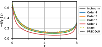
Figure 5: Single particle Green’s function $G_{11}(\tau)$ for the two-band Kanamori model [Eq. (3)] with off-diagonal hybridization at $\beta=8$. The inchworm quasi Monte Carlo result (solid lines) is compared to the exact result from exact diagonalization (dashed yellow line) and the 1st, 2nd, and 3rd order result of bold pseudo-particle self-consistent perturbation theory using the discrete Lehmann representation (PPSC-DLR) [44] (thin dashed lines).

The inchworm approach is not limited to computing single particle response functions and is able to compute arbitrary dynamical response functions [24]. As an example we study the spin-polarized Anderson impurity model with action $\mathcal{S}_{B}=\sum_{\sigma=\uparrow,\downarrow}\mathcal{S}[c_{\sigma},c^{\dagger}_{\sigma}]-\int_{0}^{\beta}\!\!d\tau\,Bc^{\dagger}_{\uparrow}(\tau)c_{\uparrow}(\tau)$ where the field $B=2$ couples to the spin-up component and $\mathcal{S}[c_{\sigma},c^{\dagger}_{\sigma}]$ (see Eq. 2) has a spin-diagonal hybridization function $\Delta_{\sigma}(\tau)=\Delta(\tau)$ with semi-circular density of states, bandwidth $W=2$, and hybridization $V=1/2$. Since the model is non-interacting, it amounts to a worst case scenario for strong coupling expansions like the inchworm approach, which expands in the hybridization function. The single particle Green’s function $G_{\sigma,\sigma}(\tau)=-\langle\mathcal{T}c_{\sigma}(\tau)c^{\dagger}_{\sigma}\rangle$ is shown in Fig. 6a with $G_{\downarrow\downarrow}$ half-filled and $G_{\uparrow\uparrow}$ almost unoccupied. The inchworm expression for dynamical response functions is agnostic to the kind of operators [24], so computing the transverse spin-response $\langle\mathcal{T}S_{+}(\tau)S_{-}\rangle$ is straightforward, see Fig. 6b. On the other hand, this correlator can not be sampled in partition function continuous time hybridization expansion Monte Carlo since in this case $S_{+}$ and $S_{-}$ do not commute with the local Hamiltonian [28, 29]. This limitation can, in part, be overcome by worm sampling [47, 48, 49]. However, for some higher order correlators like $\langle\mathcal{T}S_{+}(\tau)S_{-}\rangle$ also worm sampling has ergodicity problems, as shown in Fig. 6b.

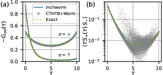
Figure 6: Panel (a): Single particle Green’s function for the spin-polarized Anderson impurity model at inverse temperature $\beta=10$. Panel (b): Out-of-plane spin-response $\langle\mathcal{T}S_{+}(\tau)S_{-}\rangle=\langle\mathcal{T}(c^{\dagger}_{\uparrow}c_{\downarrow})(\tau)(c^{\dagger}_{\downarrow}c_{\uparrow})\rangle$. The inchworm result (blue lines) at order 5 is shown together with the exact analytic solution (dotted yellow lines), and the continuous time hybridization expansion worm sampling (CTHYB+Worm) [47, 48, 49] (grey circles) where the ergodicity problem induces an extremely large variance between bins adjacent in time.

Discussion and conclusions. In conclusion, we have demonstrated a quantum impurity solver based on quasi Monte Carlo integration techniques [25, 26, 27] applied to the inchworm method [22, 23, 24]. Using quasi Monte Carlo, a $1/N$ convergence rate with the number of samples is achievable, which compares favorably to the $1/\sqrt{N}$ convergence of previous Monte Carlo methods. In order to achieve this convergence rate, the smooth Root transformation [32] of the Sobol sequence from the unit hypercube to the simplex is used, which maintains the digital net property. We demonstrate the improved convergence of our method on simple single orbital problems where exact results are available, as well as on a more challenging multi-orbital problem. These results show the usefulness of quasi Monte Carlo for achieving high accuracy of imaginary time integrals at moderate orders arising in diagrammatic expansions for quantum systems.

We also point out that stochastic inchworm quantum Monte Carlo previously has been applied to non-equilibrium real-time dynamics of quantum impurity problems, with considerable success in taming the dynamical sign problem [22, 24]. Hence, the extension of the quasi Monte Carlo integration approach to out-of-equilibrium real-time simulations is an interesting venue for further research.

Acknowledgments. HURS and IK acknowledge funding from the European Research Council (ERC) under the European Union’s Horizon 2020 research and innovation programme (Grant agreement No. 854843-FASTCORR). The computations were enabled by resources provided by the National Academic Infrastructure for Supercomputing in Sweden (NAISS) and the Swedish National Infrastructure for Computing (SNIC) through the projects SNIC 2022/1-18, SNIC 2022/6-113, SNIC 2022/13-9, SNIC 2022/21-15, NAISS 2023/1-44, and NAISS 2023/6-129 at PDC, NSC and CSC partially funded by the Swedish Research Council through grant agreements no. 2022-06725 and no. 2018-05973.

References

- Hanson et al. [2007] R. Hanson, L. P. Kouwenhoven, J. R. Petta, S. Tarucha, and L. M. K. Vandersypen, Spins in few-electron quantum dots, Reviews of Modern Physics 79, 1217 (2007).
- Scott and Natelson [2010] G. D. Scott and D. Natelson, Kondo Resonances in Molecular Devices, ACS Nano 4, 3560 (2010).
- Bloch et al. [2008] I. Bloch, J. Dalibard, and W. Zwerger, Many-body physics with ultracold gases, Reviews of Modern Physics 80, 885 (2008).
- Beenakker [1991] C. W. J. Beenakker, Theory of Coulomb-blockade oscillations in the conductance of a quantum dot, Physical Review B 44, 1646 (1991).
- Kondo [1964] J. Kondo, Resistance Minimum in Dilute Magnetic Alloys, Progress of Theoretical Physics 32, 37 (1964).
- Wilson [1975] K. G. Wilson, The renormalization group: Critical phenomena and the Kondo problem, Reviews of Modern Physics 47, 773 (1975).
- Georges et al. [1996] A. Georges, G. Kotliar, W. Krauth, and M. J. Rozenberg, Dynamical mean-field theory of strongly correlated fermion systems and the limit of infinite dimensions, Rev. Mod. Phys. 68, 13 (1996).
- Rohringer et al. [2018] G. Rohringer, H. Hafermann, A. Toschi, A. A. Katanin, A. E. Antipov, M. I. Katsnelson, A. I. Lichtenstein, A. N. Rubtsov, and K. Held, Diagrammatic routes to nonlocal correlations beyond dynamical mean field theory, Rev. Mod. Phys. 90, 025003 (2018).
- Ayral and Parcollet [2015] T. Ayral and O. Parcollet, Mott physics and spin fluctuations: A unified framework, Phys. Rev. B 92, 115109 (2015).
- Ayral and Parcollet [2016] T. Ayral and O. Parcollet, Mott physics and collective modes: An atomic approximation of the four-particle irreducible functional, Phys. Rev. B 94, 075159 (2016).
- Sun and Kotliar [2002] P. Sun and G. Kotliar, Extended dynamical mean-field theory and method, Phys. Rev. B 66, 085120 (2002).
- Kancharla et al. [2008] S. S. Kancharla, B. Kyung, D. Sénéchal, M. Civelli, M. Capone, G. Kotliar, and A.-M. S. Tremblay, Anomalous superconductivity and its competition with antiferromagnetism in doped Mott insulators, Physical Review B 77, 184516 (2008).
- Rozenberg et al. [1994] M. J. Rozenberg, G. Kotliar, and X. Y. Zhang, Mott-Hubbard transition in infinite dimensions. II, Physical Review B 49, 10181 (1994).
- Shinaoka et al. [2015] H. Shinaoka, S. Hoshino, M. Troyer, and P. Werner, Phase Diagram of Pyrochlore Iridates: All-in–All-out Magnetic Ordering and Non-Fermi-Liquid Properties, Physical Review Letters 115, 156401 (2015).
- Zhang et al. [2017] H. Zhang, K. Haule, and D. Vanderbilt, Metal-Insulator Transition and Topological Properties of Pyrochlore Iridates, Physical Review Letters 118, 026404 (2017).
- Prokof’ev et al. [1998] N. V. Prokof’ev, B. V. Svistunov, and I. S. Tupitsyn, Exact, complete, and universal continuous-time worldline monte carlo approach to the statistics of discrete quantum systems, J. Exp. Theor. Phys. 87, 310 (1998).
- Rubtsov et al. [2005] A. N. Rubtsov, V. V. Savkin, and A. I. Lichtenstein, Continuous-time quantum monte carlo method for fermions, Phys. Rev. B 72, 035122 (2005).
- Gull et al. [2011] E. Gull, A. J. Millis, A. I. Lichtenstein, A. N. Rubtsov, M. Troyer, and P. Werner, Continuous-time monte carlo methods for quantum impurity models, Rev. Mod. Phys. 83, 349 (2011).
- Werner et al. [2006] P. Werner, A. Comanac, L. de’ Medici, M. Troyer, and A. J. Millis, Continuous-time solver for quantum impurity models, Phys. Rev. Lett. 97, 076405 (2006).
- Werner and Millis [2006] P. Werner and A. J. Millis, Hybridization expansion impurity solver: General formulation and application to kondo lattice and two-orbital models, Phys. Rev. B 74, 155107 (2006).
- Haule [2007] K. Haule, Quantum monte carlo impurity solver for cluster dynamical mean-field theory and electronic structure calculations with adjustable cluster base, Phys. Rev. B 75, 155113 (2007).
- Cohen et al. [2015] G. Cohen, E. Gull, D. R. Reichman, and A. J. Millis, Taming the dynamical sign problem in real-time evolution of quantum many-body problems, Phys. Rev. Lett. 115, 266802 (2015).
- Eidelstein et al. [2020] E. Eidelstein, E. Gull, and G. Cohen, Multiorbital quantum impurity solver for general interactions and hybridizations, Phys. Rev. Lett. 124, 206405 (2020).
- Antipov et al. [2017] A. E. Antipov, Q. Dong, J. Kleinhenz, G. Cohen, and E. Gull, Currents and green’s functions of impurities out of equilibrium: Results from inchworm quantum monte carlo, Phys. Rev. B 95, 085144 (2017).
- Dick et al. [2013] J. Dick, F. Y. Kuo, and I. H. Sloan, High-dimensional integration: The quasi-Monte Carlo way, Acta Numerica 22, 133 (2013).
- Art B. Owen [2018] P. W. G. Art B. Owen, Monte Carlo and Quasi-Monte Carlo Methods, Springer Proceedings in Mathematics & Statistics (Springer International Publishing, Cham, 2018).
- Nuyens [2014] D. Nuyens, The construction of good lattice rules and polynomial lattice rules (De Gruyter, Berlin, Boston, 2014) pp. 223–256.
- Parcollet et al. [2015] O. Parcollet, M. Ferrero, T. Ayral, H. Hafermann, I. Krivenko, L. Messio, and P. Seth, Triqs: A toolbox for research on interacting quantum systems, Comput. Phys. Commun. 196, 398 (2015).
- Seth et al. [2016a] P. Seth, I. Krivenko, M. Ferrero, and O. Parcollet, Triqs/cthyb: A continuous-time quantum monte carlo hybridisation expansion solver for quantum impurity problems, Comput. Phys. Commun. 200, 274 (2016a).
- Eckstein and Werner [2010] M. Eckstein and P. Werner, Nonequilibrium dynamical mean-field calculations based on the noncrossing approximation and its generalizations, Phys. Rev. B 82, 115115 (2010).
- Sobol’ [1967] I. Sobol’, On the distribution of points in a cube and the approximate evaluation of integrals, USSR Computational Mathematics and Mathematical Physics 7, 86 (1967).
- Pillards and Cools [2005] T. Pillards and R. Cools, Transforming low-discrepancy sequences from a cube to a simplex, Journal of Computational and Applied Mathematics 174, 29 (2005).
- Maček et al. [2020] M. Maček, P. T. Dumitrescu, C. Bertrand, B. Triggs, O. Parcollet, and X. Waintal, Quantum quasi-monte carlo technique for many-body perturbative expansions, Phys. Rev. Lett. 125, 047702 (2020).
- Owen [2022] A. B. Owen, On dropping the first sobol’ point, in Monte Carlo and Quasi-Monte Carlo Methods, edited by A. Keller (Springer International Publishing, Cham, 2022) pp. 71–86.
- Seth et al. [2016b] P. Seth, I. Krivenko, M. Ferrero, and O. Parcollet, Triqs/cthyb: A continuous-time quantum monte carlo hybridisation expansion solver for quantum impurity problems, Computer Physics Communications 200, 274 (2016b).
- Krivenko et al. [2023] I. Krivenko, H. U. R. Strand, and J. Kleinhenz, QInchworm.jl: A quasi-Monte Carlo inchworm impurity solver for multi-orbital models (2023).
- Kleinhenz [2023] J. Kleinhenz, Keldysh.jl: Julia package for working with Keldysh Green’s functions (2023).
- Krivenko [2023] I. Krivenko, KeldyshED.jl: Equilibrium ED solver for finite fermionic models that can compute Keldysh Green’s functions (2023).
- Erpenbeck et al. [2023] A. Erpenbeck, W.-T. Lin, T. Blommel, L. Zhang, S. Iskakov, L. Bernheimer, Y. Núñez Fernández, G. Cohen, O. Parcollet, X. Waintal, and E. Gull, Tensor train continuous time solver for quantum impurity models, Phys. Rev. B 107, 245135 (2023).
- Note [1] Strictly speaking the rate can be proven to scale as where is the dimension for sufficiently smooth integrands.
- Boag et al. [2018] A. Boag, E. Gull, and G. Cohen, Inclusion-exclusion principle for many-body diagrammatics, Phys. Rev. B 98, 115152 (2018).
- Kanamori [1963] J. Kanamori, Electron correlation and ferromagnetism of transition metals, Prog. Theor. Phys. 30, 275 (1963).
- Georges et al. [2013] A. Georges, L. d. Medici, and J. Mravlje, Strong correlations from hund’s coupling, Ann. Rev. Cond. Mat. Phys. 4, 137 (2013).
- Kaye et al. [2023] J. Kaye, H. U. R. Strand, and D. Golež, Decomposing imaginary time Feynman diagrams using separable basis functions: Anderson impurity model strong coupling expansion, arXiv e-prints , arXiv:2307.08566 (2023).
- Kaye et al. [2022a] J. Kaye, K. Chen, and O. Parcollet, Discrete lehmann representation of imaginary time green’s functions, Phys. Rev. B 105, 235115 (2022a).
- Kaye et al. [2022b] J. Kaye, K. Chen, and H. U. Strand, libdlr: Efficient imaginary time calculations using the discrete lehmann representation, Comput. Phys. Commun. 280, 108458 (2022b).
- Gunacker et al. [2015] P. Gunacker, M. Wallerberger, E. Gull, A. Hausoel, G. Sangiovanni, and K. Held, Continuous-time quantum monte carlo using worm sampling, Phys. Rev. B 92, 155102 (2015).
- Gunacker et al. [2016] P. Gunacker, M. Wallerberger, T. Ribic, A. Hausoel, G. Sangiovanni, and K. Held, Worm-improved estimators in continuous-time quantum monte carlo, Phys. Rev. B 94, 125153 (2016).
- Wallerberger et al. [2019] M. Wallerberger, A. Hausoel, P. Gunacker, A. Kowalski, N. Parragh, F. Goth, K. Held, and G. Sangiovanni, w2dynamics: Local one- and two-particle quantities from dynamical mean field theory, Comput. Phys. Commun. 235, 388 (2019).