Improving Performance in Colorectal Cancer Histology Decomposition using Deep and Ensemble Machine Learning

Abstract

In routine colorectal cancer management, histologic samples stained with hematoxylin and eosin are commonly used. Nonetheless, their potential for defining objective biomarkers for patient stratification and treatment selection is still being explored. The current gold standard relies on expensive and time-consuming genetic tests. However, recent research highlights the potential of convolutional neural networks (CNNs) in facilitating the extraction of clinically relevant biomarkers from these readily available images. These CNN-based biomarkers can predict patient outcomes comparably to golden standards, with the added advantages of speed, automation, and minimal cost. The predictive potential of CNN-based biomarkers fundamentally relies on the ability of convolutional neural networks (CNNs) to classify diverse tissue types from whole slide microscope images accurately. Consequently, enhancing the accuracy of tissue class decomposition is critical to amplifying the prognostic potential of imaging-based biomarkers. This study introduces a hybrid Deep and ensemble machine learning model that surpassed all preceding solutions for this classification task. Our model achieved 96.74% accuracy on the external test set and 99.89% on the internal test set. Recognizing the potential of these models in advancing the task, we have made them publicly available for further research and development.

[inst1]organization=University of Jyväskylä, Faculty of Information Technology, addressline=, city=Jyväskylä, postcode=40014, country=Finland

[inst3]organization=University of Helsinki, Faculty of Science, Department of Computer Science, , city=Helsinki, country=Finland

[inst4]organization=University of Helsinki, Faculty of Agriculture and Forestry, Department of Food and Nutrition, , city=Helsinki, country=Finland

[inst5]organization=University of Jyväskylä, Faculty of Mathematics and Science, Department of Biological and Environmental Science, addressline=, city=Jyväskylä, postcode=40014, country=Finland

[inst7]organization=University of Turku, Institute of Biomedicine, Cancer Research Unit, addressline=, city=Turku, postcode=20014, country=Finland

[inst8]organization=Turku University Hospital, FICAN West Cancer Centre, addressline=, city=Turku, postcode=20521, country=Finland

[inst10]organization=University of Jyväskylä, Department of Biological and Environmental Science, addressline=, city=Jyväskylä, postcode=40014, country=Finland

[inst11]organization=Hospital Nova of Central Finland, Department of Pathology, addressline=, city=Jyväskylä, postcode=40620, country=Finland

1 Introduction

Cancer comprises diseases marked by rapid, uncontrolled growth of abnormal cells that form malignant tumors. These cells can detach, spread, and form new tumors in distant body parts, a process known as metastasis, which is the primary cause of cancer-related deaths [1]. The World Health Organization reports that cancer is a leading global cause of death, responsible for one in six deaths [2]. The most common areas for cancer to initially develop are the breast, lung, colon, and prostate.

Colorectal Cancer (CRC) is the third most common yet second deadliest cancer [3]. American Cancer Society data indicates 56% of patients are diagnosed at stages where cancer has begun to metastasize [4, 5]. Early detection and treatment are paramount [6]. Machine vision advancements, especially through deep neural networks [7], have improved automatic cancer and other disease classification [8, 9, 10, 11, 12, 13]. Despite the technological progress, healthcare professionals still need to examine histologic samples to confirm diagnoses and assess tumor stages. Hematoxylin and Eosin (H&E) staining is typically used to highlight key histopathological features in these tissues[14, 15].

CRC patients are categorized into different groups to tailor their treatment and surveillance strategies. Grouping relies on multiple factors, including clinical outcomes, tumor genetics, quantitative biomarkers, clinical data, and histopathological and molecular analyses of the tumor. Many biomarkers stem from molecular and genetic tests [16, 17, 18, 19]. Recent insights into tumor immunology have revealed the critical role of the tumor microenvironment in tumor growth. Therefore, discovering novel predictive and prognostic biomarkers that effectively identify tumor characteristics is crucial.

In recent times, the first quantitative biomarkers based on deep learning have been extracted from H&E stained whole-slide images [10, 8, 20, 21, 22, 23]. Kather and colleagues [8] were the first to use deep learning to identify a biomarker for stages III and IV of CRC. This novel biomarker exhibited performance comparable to the existing gold standards for determining CRC outcomes [24, 25] and could be automatically generated from images, saving time and resources. Conversely, known biomarkers (MSI, BRAF and KRAS) were also predicted [26] with deep learning transformers [27]. The approach greatly surpassed current methods for detecting microsatellite instability in surgical samples and achieved clinical-level accuracy in colorectal cancer biopsies, a significant finding in the field [28].

In their seminal research, Kather et al.[8] applied convolutional neural networks (CNNs) [29] to identify nine distinct tissue classes from HE-stained whole-slide images. Their methodology led to a noteworthy classification accuracy of 94.3% on their external testing data. They then compiled output layer neuron activations into a single weighted score, named ’Deep Stroma’, and tested this new CNN-biomarker for outcome prediction in new patient cohorts. They discovered that the ’Deep Stroma’ score was a significant prognostic factor, especially in patients with advanced tumor stages (UICC IV). The CNN-biomarker was significantly prognostic in all tumor stages, while manual pathologist annotations and cancer-associated fibroblast (CAF) scores were not. Kather and his team prioritized the model with the highest accuracy, as it directly enhanced the quality and applicability of the new prognostic CNN-biomarker.

Subsequent studies [30, 31, 32, 33, 34, 34, 35, 36, 37] have made notable strides in improving accuracy. Nevertheless, some have either reported results not surpassing the original Kather, et al.[8] model or faced challenges with incompatible output layer specifications and different validation methodologies. In our prior study [38], we refined the model originally proposed by Kather et al.[8], achieving results superior to those previously reported. Building on that foundation, the current study introduces a new model that improves classification accuracy for this task and further surpasses previous solutions. Utilizing the EfficientNetV2 CNN architecture [39] in conjunction with the random forest ensemble algorithm [40], we introduce a hybrid deep and ensemble model.

2 Materials and Methods

In this Methodology section, we detail our research process, outlining our data handling, image augmentation techniques, and the use of Convolutional Neural Networks. As shown in Figure 1 we focused on EfficientNetV2 for image classification, supplemented by the Random Forest method to generate the final deep ensemble model for refined predictions. The process began with the acquisition of HE-stained colorectal cancer data as the first step. In the second step, EfficientNetV2 models were trained for tissue classification. Once the best-performing EfficientNetV2 model was identified, it was frozen in the third step, and a new random forest classifier was trained using the learned features. The fourth step involved evaluating the hybrid model using both test and external datasets. Additionally, results from this model were compared with those obtained from AutoKeras.

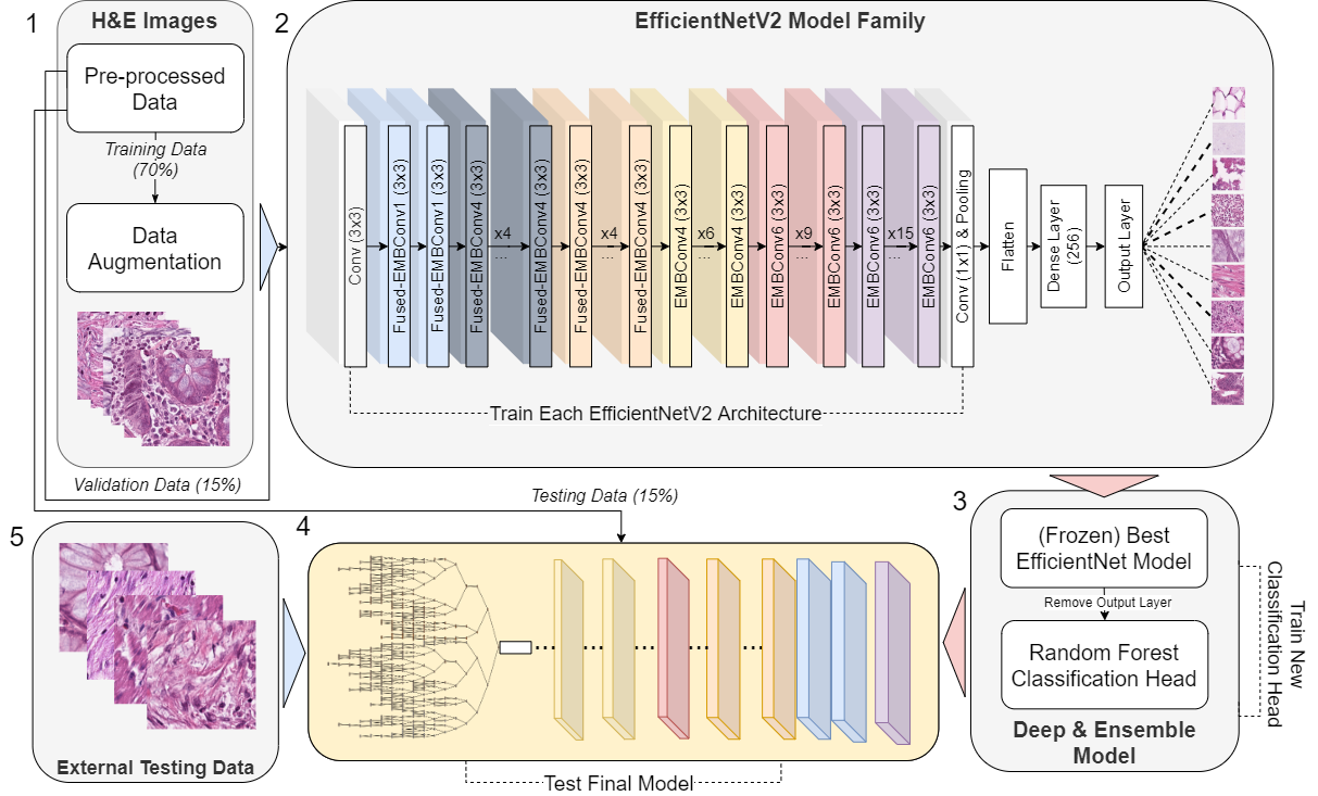
Figure 1: Methodological Pipeline for Model Development. Blue arrows indicate data flow, red arrows represent model transfer, and numerical markers show the operational sequence.

2.1 Data Acquisition and Pre-processing

The data utilized in this study were collected by the National Center for Tumor Diseases (NCT) in Heidelberg, Germany, and the University Medical Center Mannheim (UMM) in Mannheim, Germany. This comprehensive dataset has been made publicly available by Kather et al.[8] and consists of 100,000 non-overlapping image tiles derived from 86 HE-stained tissue slides[41]. The image tiles, each measuring 224 x 224 pixels, were normalized using the Macenko method[42]. These images span nine distinct classes: 1) adipose tissue (ADI); 2) background (BACK); 3) debris (DEB); 4) lymphocyte (LYM); 5) mucus (MUC); 6) smooth muscle (MUS); 7) normal colon mucosa (NORM); 8) cancer-associated stroma (STR); 9) CRC Epithelium (TUM). A detailed breakdown of the class distribution can be found in Figure 2, and representative images for each class are displayed in Figure 3.

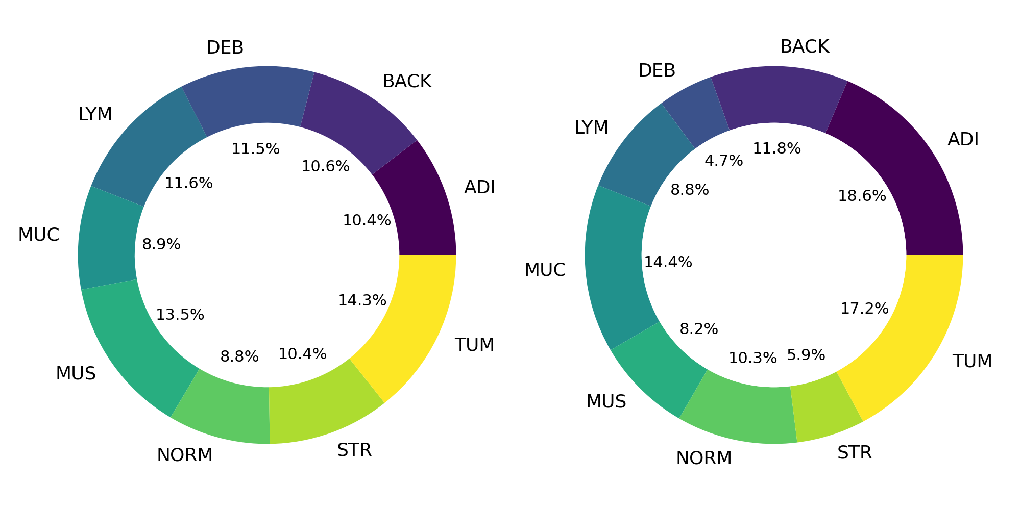
Figure 2: Figure 2 depicts the source (pre-split) data on the left, with the inner ring showing training data percentages and class labels on the outer ring. The right side presents analogous details for the external-testing data.

The dataset was partitioned into a training, validation, and testing set containing 69996, 14995, and 15009 images, respectively. This distribution corresponded to 70% of the original data for training, 15% for validation, and 15% for testing. We also incorporated the external testing set from the original work by Kather et al.[8], consisting of 25 CRC HE slides from the NCT biobank, providing an additional 7180 image patches, code named (CRC-VAL-HE-7K)[41]. Figure 3 visualizes the number of images in each class for the training and external testing data.

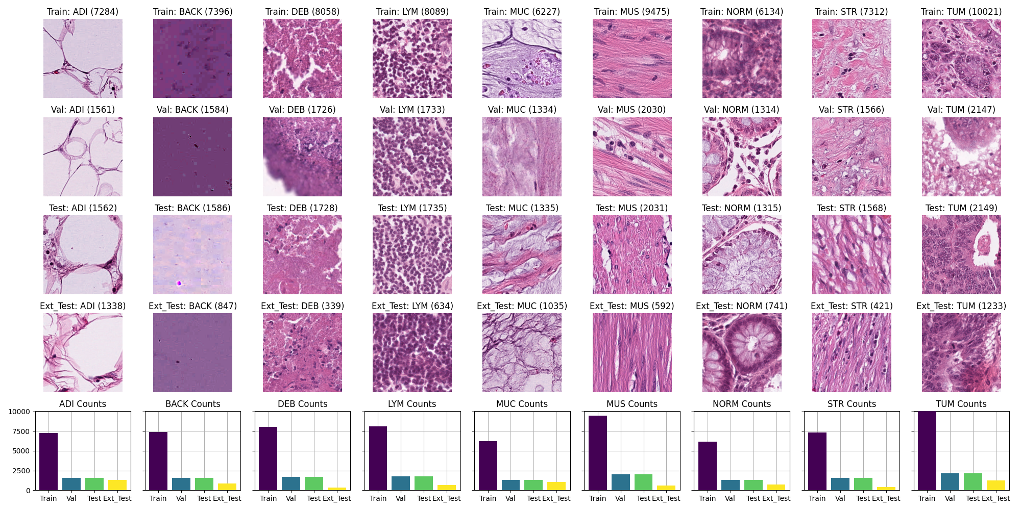
Figure 3: Image tile examples and image counts for each data partition set (rows), exTest refers to external test data.

2.2 Data Augmentation

Data augmentation, a technique to artificially enhance the diversity of training images [43], is applied by randomly transforming some images before they are fed into the training. Simple examples include random image rotation or shifting. When using multiple augmentations, the methods are combined to increase the possible variations. In this study’s context, we employed six data augmentation methods bundled in the ’advanced’ preset of the Deep Fast Vision Repository [44]. Each method and its specific configuration is detailed in Table 1.

Table 1: A detailed description of the various image augmentation techniques utilized during the training of our neural networks.

Augmentation Technique	Technique Explanation	Training Settings
Rotation	Rotates the image in the plane.	Allows image rotation up to a maximum of 40 degrees.
Width Shift	Shifts the image horizontally.	Allows a shift of up to +- 45 pixels along the width.
Height Shift	Shifts the image vertically.	Allows a shift of up to +- 45 pixels along the height.
Shear	Distorts the image by ”stretching” it either horizontally or vertically, providing a ’skewed’ perspective.	Shearing of the image is allowed up to a maximum angle of 0.2 degrees.
Zoom	Changes the image’s apparent distance, making it seem closer or farther away.	Allows for a maximum zoom of up to 20%.
Horizontal Flip	Creates a mirrored version of the image, providing a reflection along the vertical axis.	Only horizontal flipping is supported.

2.3 Convolutional Neural Networks

One of the bedrocks of the recent surge in deep learning is the Convolutional Neural Network (CNN) [29]. A particular type of neural network, CNNs are often deployed for tasks in computer vision. They utilize the operation of convolution between an input and a filter-kernel. The kernels or filters are moved over the inputs to create feature maps, which represent highlighted features of the input. Different feature maps can be aggregated to form higher-level feature maps corresponding to more complex concepts. In a formal context [45], given an image I with dimensions $m\times n$ and a filter-kernel K with dimensions $q\times r$, we generate the feature map F via convolution along the axes $m,n$ with the kernel K as follows:

$$\textbf{{F}}(m,n)=\sum_{q}\sum_{r}\textbf{{I}}(m,n)\textbf{{K}}(m-q,n-r)$$ (1)

Typically, the values in the feature map undergo a transformation by an activation function. One common example is the rectified linear unit activation function [46] (ReLu) which transforms all negative values to zero. This technique contributes to computational efficiency by zeroing-out unnecessary values. The ReLu activation for a given feature map value $x$ is defined as:

$$f(x)=\max(0,x)$$ (2)

In addition to using activation functions, a common practice is to implement max pooling. This operation reduces the size of the convolution result, and with sequential use of convolution and max pooling, the feature size continues to diminish. For image I of dimensions $m\times n$, the max-pooled value ${l(m_{I})}$ corresponding to dimension $m$ can be defined as:

$$l(m_{I})=\lfloor\frac{{m_{I}}-p}{s}\rfloor+1$$ (3)

Here, $m_{I}$ is only dimension $m$ from image I, $p$ refers to the size of the pooling window, and $s$ represents the stride value.

2.4 EfficientNet Architecture

EfficientNet [47] is a model that has gained traction in machine learning applications in recent years. The architecture of EfficientNet has been designed to systematically scale all dimensions of depth, width, and resolution.

The underlying idea of EfficientNet is based on the compound scaling method. This strategy aims to maintain a balance between the network depth (how many layers it has), width (how wide are the layers), and resolution (input image size). A set of fixed scaling coefficients guides this balance. Formally, for a baseline EfficientNet-B0, if $\alpha,\beta,\gamma$ are constants which maintain the balance, and $\phi$ is the user-specified coefficient, we can scale depth $d$, width $w$, and resolution $r$ of the network according to:

$$d=\alpha^{\phi}d_{0},\quad w=\beta^{\phi}w_{0},\quad r=\gamma^{\phi}r_{0}$$ (4)

Here, $d_{0},w_{0},r_{0}$ are the depth, width, and resolution of the base model, respectively.

A core component of EfficientNet is the MBConv block, inspired by the MobileNetV2[48] architecture. This block applies a series of transformations: a $1\times 1$ convolution (expansion), followed by a depth-wise convolution (represented by a depth-wise separable convolution kernel D), a Squeeze-and-Excitation (SE) operation [49], and another $1\times 1$ convolution (projection). For an input image I, the transformation of the MBConv block, $T_{MB}$, can be represented as:

$$T_{MB}(\textbf{{I}})=\textbf{{K}}_{2}\ast SE(\textbf{{D}}\ast(\textbf{{K}}_{1}\ast\textbf{{I}}))$$ (5)

In this equation, $\ast$ represents the convolution operation, $\textbf{{K}}_{1}$ and $\textbf{{K}}_{2}$ are the $1\times 1$ convolutional filters, D represents the depth-wise convolutional filter, and $SE(\cdot)$ denotes the Squeeze-and-Excitation operation. Each convolution is followed by an activation function. This efficient use of computational resources within the MBConv block, especially through the depth-wise convolution and the SE block, contributes significantly to the excellent performance of EfficientNet.

EfficientNetV2 [39] introduces several key changes to the original EfficientNet architecture. The depth, width, and resolution scaling remain the same as in the original EfficientNet. However, the use of the Fused-MBConv block, which combines the initial $1\times 1$ convolution and the depth-wise convolution into a single $3\times 3$ convolution operation, and then applies the Squeeze-and-Excitation (SE) operation followed by a final $1\times 1$ convolution, is a significant modification.

The transformation of the Fused-MBConv block, $T_{FMB}$, can be expressed as:

$$T_{FMB}(\textbf{{I}})=\textbf{{K}}_{2}\ast(SE(\textbf{{K}}_{f}\ast\textbf{{I}}))$$ (6)

In this equation, $\textbf{{K}}_{f}$ is the $3\times 3$ convolutional filter that combines the initial $1\times 1$ convolution and the depth-wise convolution, $\mathbf{K}_{2}$ is the final $1\times 1$ convolutional filter and $SE(\cdot)$ denotes the Squeeze-and-Excitation operation.Each convolution, followed by an activation, is part of a block that may contain a skip connection.

Another key change in EfficientNetV2 is the progressive learning method, which adaptively adjusts the regularization and image size during training. EfficientNetV2 models to train faster and achieve better parameter efficiency than the original EfficientNet, even outperforming transformer models on key vision tasks, such as Image-Net Classification. Figure 4 illustrates the EfficientNetV2’s base architecture (B0). Complementing this, Table 2 enumerates each family variant from the Keras documentation[50], detailing their ImageNet accuracy and base parameter count.

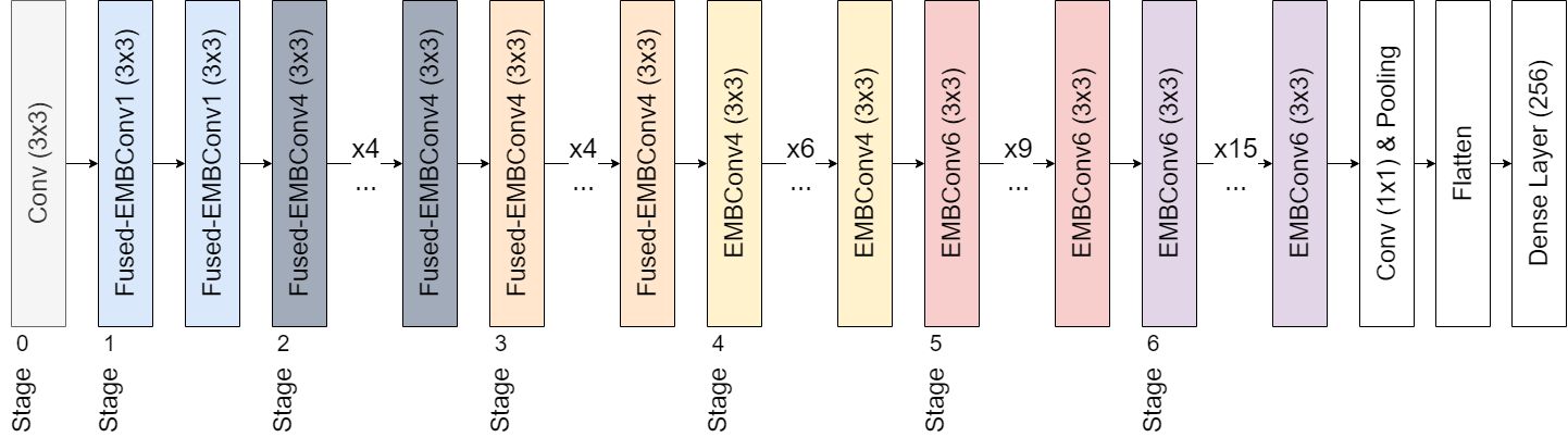
Figure 4: Diagram illustrating the integrated architecture of the base EfficientNetV2 and our modifications after the pooling layer

In our experiment, we extensively explored the EfficientNetV2 family of models, ranging from the relatively compact EfficientNetV2-B0 to the more complex EfficientNetV2-M. We supplemented the architecture by incorporating a flattening layer, followed by a densely connected layer of 256 neurons. This dense layer utilized an Exponential Linear Unit (ELU) as its activation function, set before the final output layer. For the training process, we employed Categorical Cross-Entropy Loss to optimize the model’s performance, and trained for 15 epochs each model family. The minimum validation loss was used as the early stopping criterion. All model training was performed with the Deep Fast Vision repository. The optimizer used was Adam [51], with a learning rate of $2\times 10^{-5}$ and a batch size of 32.

Table 2: Comparison of EfficientNetV2 variants. ImageNet Top Accuracy refers to the model’s performance on the ImageNet validation dataset benchmark.

Model	ImageNet Top-1 Accuracy	ImageNet Top-5 Accuracy	Base Parameters
EfficientNetV2B0	78.7%	94.3%	7.2M
EfficientNetV2B1	79.8%	95.0%	8.2M
EfficientNetV2B2	80.5%	95.1%	10.2M
EfficientNetV2B3	82.0%	95.8%	14.5M
EfficientNetV2S	83.9%	96.7%	21.6M
EfficientNetV2M	85.3%	97.4%	54.4M

2.5 Random Forests

Random Forests [40] (RF) is an ensemble machine learning method that leverages multiple decision trees to make predictions. Its robustness stems from combining a multitude of weak learners, the individual trees, to form a strong learner, the Random Forest. The most typical form of decision tree uses binary decisions based on feature thresholds to make predictions. The prediction of a single decision tree, $T_{d}$, on an input vector I, can be mathematically expressed as:

$$T_{d}(\textbf{{I}})=\sum_{i=1}^{n}v_{i}\delta(f_{i}(\textbf{{I}})<t_{i})$$ (7)

In this equation, $n$ is the total number of nodes in the tree, $v_{i}$ is the predicted value for the $i$-th node, $f_{i}(\textbf{{I}})$ represents the $i$-th feature of the input vector I, $t_{i}$ is the threshold for the $i$-th node, and $\delta$ is the indicator function.

A Random Forest aggregates the predictions from $D$ decision trees to make a final prediction. For regression problems, the decision tree outputs are typically averaged, while for classification, they are aggregated through a majority vote (mode). Formally, the prediction of a Random Forest, $F_{D}$, on an input vector I, can be represented as:

$$F_{D}(\textbf{{I}})=\frac{1}{D}\sum_{d=1}^{D}T_{d}(\textbf{{I}})$$ (8)

In this equation, $T_{d}(\textbf{{I}})$ is the output of the $d$-th decision tree for input vector I, and $D$ is the total number of decision trees in the forest. The Random Forest model’s strength lies in its ability to reduce overfitting compared to a single decision tree by averaging the results over many trees. In our experiment, we employed 400 estimators and default parameters from the scikit-learn library [52]. Ultimately, the best-performing EfficientNet (Deep) model, determined by validation accuracy, had its classification head replaced by the Random Forest. After training and validating the RF, it was evaluated once on the test and external test sets.

2.6 t-Distributed Stochastic Neighbor Embedding

The t-Distributed Stochastic Neighbor Embedding (t-SNE)[53] is a tool for visualizing high-dimensional data in a lower-dimensional space, often two or three dimensions. It is particularly effective for visualizing complex data structures, such as those produced by deep learning models, in a way that preserves the relationships and structures within the data.

In our experiment for visualizing the external test data from the trained model, we used two dimensions with an automatic learning rate on the dense layer before the output layer of the best EfficientNetV2 model. Additionally, we sampled 160 examples per class from the lower-dimensional space and rasterized[54, 55]the projected space. These two approaches can be seen in results Figure 8, while Figure 9 demonstrates the replacement of all data points with their corresponding whole-slide image patches.

2.7 Automatic Machine Learning Repository

Automatic Machine Learning (Auto-ML) refers to automating the end-to-end process of applying machine learning to real-world problems. Auto-ML has been particularly beneficial in cases where domain expertise is scarce and there is a pressing need to get insights from data. Regarding transfer learning auto-ml for vision, only two libraries exist, AutoKeras[56] and Deep Fast Vision[44]. In our experiment, we used both libraries for the vision task.

2.7.1 AutoKeras Configuration

AutoKeras[56] is an open-source Auto-ML library for deep learning, built on top of Keras and offers functionalities like automatic model selection and hyperparameter tuning. The library can handle various data types, including images, text, and structured data. For our experiment, we initiated a search incorporating instance normalization block, image-augmentation, ResNet V2 blocks pre-trained with ImageNet, all followed by flatten and dense layer blocks. We trained for 15 epochs and ran a maximum of 6 trials; early stopping (with restore best weights) was employed, and the search focused on validation loss.

2.7.2 Deep Fast Vision Configuration

Deep Fast Vision [44] is an open-source Auto-ML library designed to prototype deep transfer learning vision models rapidly. It is built around Keras[50] and TensorFlow[57] and offers automatic setups for loss/target types, generators, output layers, and data augmentation. It also manages the saving and loading of best weights, class weights calculation, validation curves, and confusion matrices, as well as configuring dense layers and regularization. Pre-training new dense layers before unfreezing any transfer architecture is also automated. In our experiment, all automations except for dense layer pre-training were used. Post-training dense layer features connected to a random forest algorithm were extracted using the same library. All generated models and components are exported and can be accessed as if generated from Tensorflow or Keras for further use or modification.

3 Results

3.1 Classification

As presented in Table 3, we evaluated the performance of a series of models, including several EfficientNet architectures (without testing), the final hybrid model, and an AutoKeras baseline. The table provides a comprehensive summary of the training, validation, testing accuracy scores, and parameter counts for each model. Notably, the EfficientNet models consistently showcased a rise in accuracy scores corresponding to an increase in model complexity, emphasizing the positive association between the number of parameters and model performance. Among the investigated models, EfficientNetV2M emerged with the highest validation accuracy. This deep model subsequently served as the basis for our hybrid model, complemented by a Random Forest (RF) classification head. Our hybrid model underwent further evaluations on internal and external test sets to ascertain its robustness and applicability. The model accuracy scores of 99.89% on the internal test set and 96.74% on the external test set. In comparison, the AutoKeras baseline model could not match the accuracy levels exhibited by the hybrid model.Table 4 offers a detailed comparative analysis, juxtaposing the performance metrics of our model with those from other studies. Notably, our approach achieved superior results in both internal and external testing datasets.

Table 3: Comparison of accuracy and parameter count across different EfficientNet models and the AutoKeras baseline model.

Model Name	Training Accuracy	Validation Accuracy	Testing Accuracy	External Testing Accuracy	Parameter Count (M)
EfficientNetV2B0	99.5%	99.57%	-	-	21.98
EfficientNetV2B1	99.5%	99.73%	-	-	22.99
EfficientNetV2B2	99.51%	99.73%	-	-	26.43
EfficientNetV2B3	99.59%	99.75%	-	-	32.20
EfficientNetV2S	99.68%	99.79%	-	-	36.39
EfficientNetV2M	99.72%	99.8%	-	-	69.21
EfficientNetV2M + RF	100%	99.91%	99.89%	96.74%	69.21
AutoKeras Model (Baseline)	100%	98.47%	98.52%	94.21%	26.77

As shown in Figure 5, using the one-vs-all scheme, our hybrid model and the AutoKeras baseline model’s performance on the external testing set were assessed using the Area Under the Receiver Operating Characteristic (ROC) Curves. Our hybrid model displayed superior performance across all classes. It achieved the maximum AUC score of 1.00 for ADI, BACK, DEB, LYM, MUC, MUS, NORM, and TUM classes. For the STR class, the AUC slightly dropped, and our model registered a score of 0.97. On the contrary, the AutoKeras baseline model, while demonstrating high AUC scores for ADI, BACK, MUC, NORM, and TUM, showed diminished performance for the remaining classes. The most notable dip was observed for class STR, registering an AUC of 0.89. Notably, the ROC curve for the AutoKeras baseline model intersected with the baseline after the 0.8 threshold. This intersection was not observed in the ROC curves of the hybrid model.

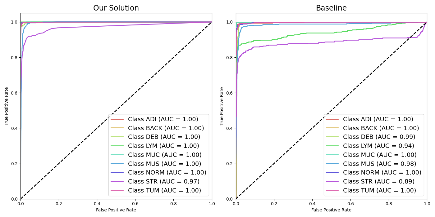
Figure 5: Benchmarking EfficientNetV2M + RF hybrid vs. AutoKeras using one-vs-all ROC curves.

Table 4 comprehensively compares accuracy scores across all relevant studies that employed the original training and external testing data. As shown, our model demonstrated superior performance, surpassing all other studies.

Table 4: Comparative analysis of accuracy metrics and validation techniques across Studies.

Study	Training Set (TR)	Validation Set (V)	Test Set (T)	Validation Approach	External Test Set (T2)
Ours	100%	99.91%	99.89%	TR-V-T-T2	96.74%
Prezja, et al.[38]	99.4%	99.3%	99.5%	TR-V-T-T2	95.6%
Kather et al.[8]	-	-	98.7%	TR-V-T-T2 TR-T2	94.3%
Peng et al.[30]	-	-	-	TR-V-T-T2	95%
Qi et al.[31]	-	99%	-	TR-V-T2	95%
Shen et al.[32]	-	-	-	TR-V-T2	94.8%
Wang et al.[33]	-	-	-	TR-V-T2	94.8%
Yang et al.[34]	-	-	-	TR-V-T2	91.1%
Yang et al.[58]	-	-	-	TR-V-T2	86.4%

Furthermore, our study stands out as the only one providing a complete and transparent report of errors across all stages - from training through to external testing. In evaluating these studies, studies [59, 60] that did not use valid validation approaches, such as the absence of validation and testing data to detect overfitting, including the search for parameters and hyperparameters on external testing data, are not eligible for comparison. Moreover, instances that employed techniques like few-shot learning and testing [35], shuffling of external testing data within training data [36], and using external testing as validation and testing with their own testing data [61], also don’t meet the criteria for a comparative analysis.

Figure 6 demonstrates exceptional performance across most classes, with the vast majority of predictions falling on the diagonal, signifying correct classifications. Class BACK, LYM, and NORM are particularly noteworthy, which were nearly perfectly classified. However, the model exhibits some confusion between classes MUC-MUS, and STR-MUS, suggesting shared features or characteristics that led to these misclassifications.

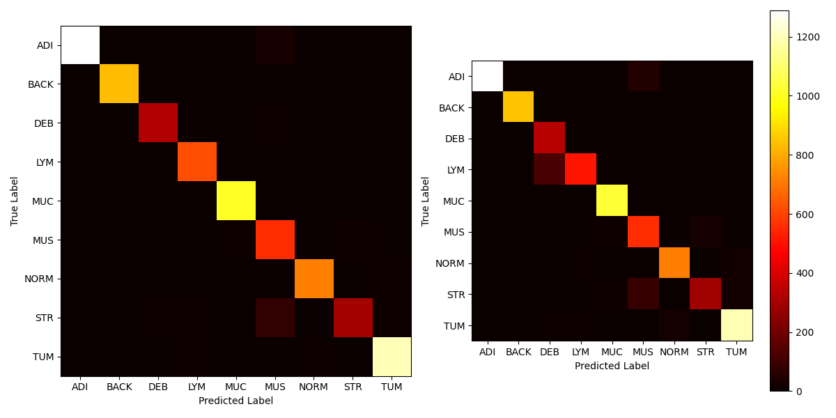
Figure 6: Confusion matrices for external testing: Hybrid Model (left), AutoKeras baseline (right). Identical color format as Kather et al.[8] for direct comparison.

The confusion matrix from the original study conducted by Kather et al. revealed certain areas of confusion between particular classes, specifically LYM-DEB, MUS-MUC, NORM-TUM, TUM-STR, and STR-MUSC-MUC. When we compare this with the confusion matrix generated by our hybrid model, we see substantial improvements in classification accuracy, especially in the problematic areas identified in Kather’s study. Figure 6 (on the left) shows that our model successfully eliminated most of these previously reported confusions. For instance, our model has resolved the confusion between LYM-DEB, indicating its improved ability to distinguish between these two classes. Similarly, the confusion between MUS-MUC and NORM-TUM seen in Kather’s study has also been resolved. One of the most substantial improvements was observed in the classification of LYM, where our model demonstrated almost perfect classification accuracy. In figure 6 (on the right), the AutoKeras model, still achieving overall solid performance, underperformed in several areas relative to the hybrid model. Specifically, there is apparent confusion between classes DEB-LYM, and STR-MUS. It is also worth noting that, unlike the hybrid model, the AutoKeras model made several misclassifications between classes TUM and NORM.

The hybrid model’s superior performance is most noticeable when dealing with classes ADI, MUS, LYM, NORM, and STR, suggesting that its architecture may be more adept at recognizing the nuanced features that distinguish these classes. These features are relevant to the Deep Stroma score calculation proposed by Kather.

In the t-SNE visualization of the high-dimensional feature space (Figure 7), the classes align almost seamlessly around the tumor (TUM) class at the approximate center. This near-optimal separation of classes demonstrates the effectiveness of the hybrid model in distinguishing between various histopathological types. Notably, there is no observed fragmentation within the classes, underlining the consistency of the learned features even as a two-dimensional projection. Moreover, the relative positioning of the classes aligns with histopathological anticipations. The TUM and normal (NORM) tissues, displaying histological similarities, are situated adjacently on the t-SNE map. Analogously, the proximity of the stroma (STR) and muscle (MUS) classes suggests vector space congruence. Transitioning the t-SNE map into a rasterized depiction preserves relative inter-class distances and condenses the visualization by eliminating inter-point space, enabling a more compact visualization of class distributions. Figure 8 illustrates a single instance from each class closest to each class mean as projected by t-SNE. Concurrently, we subsample the t-SNE space with 160 samples per class to build a rasterized representation, substituting data-points with corresponding images. Figure 9 follows the same pattern but without sub-sampling, using all external test data.

Overall, these results demonstrate the robustness of the hybrid model’s feature extraction and highlight its potential to provide clinically relevant insights.

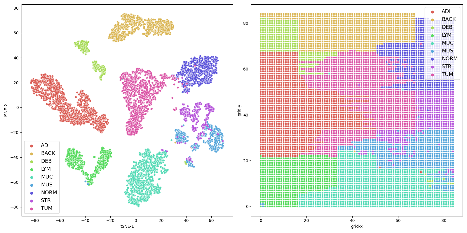
Figure 7: Left: t-SNE projection illustrating near-optimal class separation with TUM class at center. Right: Rasterized t-SNE map preserving relative inter-class distances and eliminating inter-point distance.

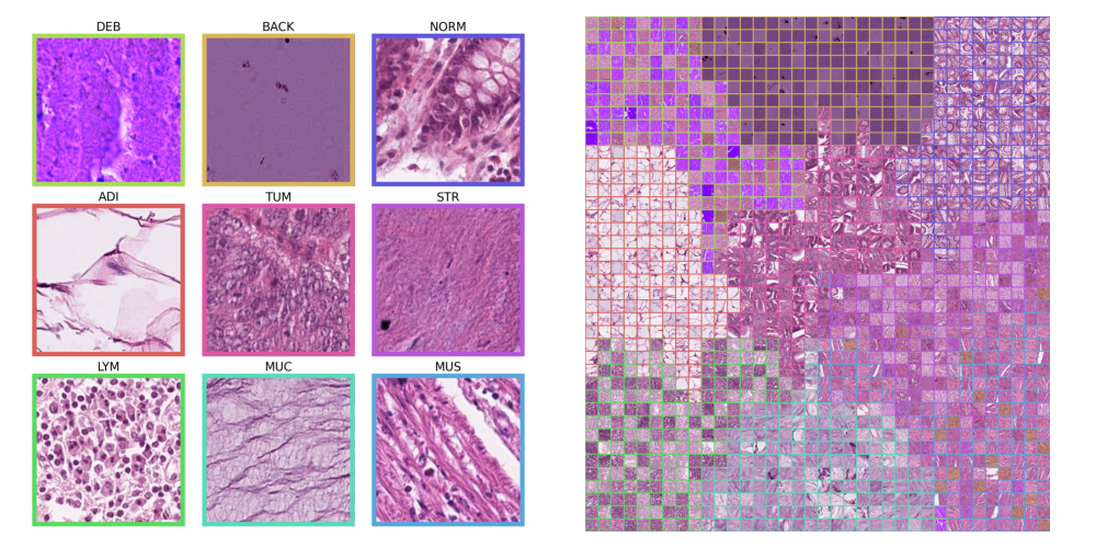
Figure 8: Left:Nearest intra-class image to class mean in the t-SNE projection. Right: Rasterized t-SNE space with 160 samples per class, data points replaced with images. Boundary colors indicate class origin.

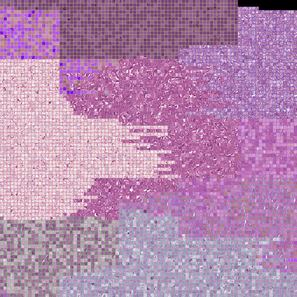
Figure 9: Rasterized t-SNE visualization of all external test data showing class distributions. Black indicates blank grid space, boundary colors denote class origin. The full resolution is made available under data availability.

4 Discussion

The present study was designed to advance the decomposition classification of colorectal cancer by developing a novel hybrid model. Our methodology integrated EfficientNetV2M and Random Forest (RF) techniques, with the results demonstrating the model’s superior performance over previously proposed solutions (Table 4). This was achieved by combining the strengths of both deep learning and traditional ensemble machine learning. In addition to achieving high accuracy rates, our hybrid model demonstrated superior performance across all classes when assessed using the Area Under the Receiver Operating Characteristic (ROC) Curves in a one-vs-all scheme (Figure 5). The hybrid model achieved the maximum AUC score of 1.00 for classes ADI, BACK, DEB, LYM, MUC, MUS, NORM, and TUM. While the model performance slightly dropped for the STR class, it still registered an AUC of 0.97. The confusion matrices demonstrated the hybrid model’s improved ability to correctly classify various histopathological types, even those that presented difficulties in previous studies, such as the original study by Kather et al[8].

In terms of data augmentation and validation, our findings suggest that robust data augmentation is a powerful tool for mitigating overfitting when paired with an appropriate validation technique. This conclusion is consistent with established practices, as data augmentation is a commonly used method in numerous classification studies. As illustrated in Table 4, however, there is considerable variation in validation methods, which poses a challenge when validation, testing, and external testing datasets are missing. The practice of validation in this context could be significantly improved by adopting a standardized approach. From a limitation perspective, the training of such systems necessitates a substantial volume of annotated data. For potential advancements in these systems, the annotation of even more data by medical professionals may be required. Notably, several studies [32, 34, 60] are still pending peer review, thereby constraining their comparative scope.

In reflecting upon the prevailing CRC scientific literature, we have noted considerable advancements achieved over a comparably short time. However, this progress has not been devoid of limitations. Firstly, our survey identified a distinct lack of uniformity in the evaluation methodologies employed across different systems. Emphasizing consistency and adherence to best practices during evaluation is crucial for reducing biases and enabling direct system comparisons. Moreover, estimates for metrics such as label noise are absent. Ascertaining estimates for label noise could be pivotal in establishing a benchmark for future comparative analyses.

In our study, the hybrid model’s deep section was trained using our new Deep Fast Vision open-source library [44], whereas the baseline employed AutoKeras [56]. Both these libraries uniquely leverage AutoML in vision-related contexts with transfer learning capabilities. The hybrid model demonstrated improvement in scores compared to AutoKeras. Although AutoKeras employs ImageNet pre-trained blocks, such blocks function independently, and only low-level features are loaded. On the contrary, Deep Fast Vision utilizes the entire hierarchy of learned features from already validated architectures. This methodology gives Deep Fast Vision an expected early advantage over AutoKeras, allowing it to harness the transfer learning capability of previously validated deep learning models.

Concerning the quality of microscope images, factors such as the slide’s quality and the presence of artifacts or pixel noise could significantly contribute to misclassifications. Normalization and contrast enhancement processes performed on tiles before their entry into the classifier might accentuate pixel noise or other non-tissue artifacts, such as dust or hair, thereby potentially skewing results. The ’Picasso’ effect [62] may compound these distortions in Convolutional Neural Networks (CNNs). Furthermore, instances, where a tile contains minimal or no relevant tissue and isn’t labeled as background could also instigate misclassifications. Incorporating a background class can somewhat mitigate these issues, but this effect is only partial, and similar errors would be anticipated. Future systems could benefit from introducing pixel noise during the augmentation phase, ideally in a randomized manner and with replacement. Randomization and replacement are critical to prevent the introduction of biases and potential overfitting by the classifier. Lastly, the focus factor (’blur’) can also influence results, particularly when it coexists with pixel noise. As a preventative measure, further augmentation involving a variety of blur intensities might be beneficial. Such recommendations are particularly crucial given the variability in focus and quality across different patient slides.

In our previous study [38], we highlighted the need for a deeper analysis of classifier probability profiles [63]. While Kather’s approach [8] pinpointed one classifier, it did not address the influence of model probability calibration on the deep stroma score. Given that different architectures can produce varying probability profiles, even with similar performance metrics, there’s a gap in understanding these profiles’ effects on deep stroma and outcome prediction. Addressing this could open new avenues for research and refine our approach to model architectures and outcome predictions. Before advancing to bio-marker extraction and patient outcome assessment, it’s imperative that these profiles undergo further validation.

In Kather, et al.[8] from which we sourced our data, there was a stringent manual review process for all slides. Slides with pronounced artifacts, be it tissue folds or tears, were set aside. This exclusion underscores an inherent gap: our models, along with others, have not been trained with these challenges. In many real-world scenarios where such artifacts may exist, the desired performance might decline, emphasizing the importance of training datasets that mirror extensive real-world challenges. While remedies like affine augmentations might provide some mitigation, they fall short of fully addressing these challenges.

5 Conclusion

Our study successfully developed a hybrid model that combines the EfficientNetV2 and Random Forest algorithms, notably advancing the task of automatic colorectal cancer tissue decomposition. Our model not only demonstrated high accuracy but also excelled in performance across all classes, as indicated by the AUC scores. It surpassed the results of all previous research in this domain, including the seminal work by Kather et al.[8].

It is imperative that this work is subjected to rigorous clinical validation before any deployment into routine clinical practice. Our research presents considerable potential in the classification of CRC slides and the prospect of improving CNN-based biomarkers that rely on classification accuracy. This improvement, in turn, could lead to improved predictions for CRC patient outcomes.

Lastly, we have made a commitment to transparency and replicability by providing unrestricted access to our models.

6 Data Availability

Materials and best models from the current study are accessible in the Google Drive repository: xxx

Author contributions statement

Conceptualization: F. P. & T.K.; Methodology: F. P.; Investigation: F. P. & T.K.; Data Curation: All authors; Formal analysis: All authors; Writing – original draft: F. P.; Writing – review & editing: All authors.

Additional information

Competing interests All authors declare that they have no conflicts of interest.

References

- [1] C.-N. Qian, Y. Mei, J. Zhang, Cancer metastasis: issues and challenges, Chinese journal of cancer 36 (1) (2017) 1–4.
- [2] WHO, Cancer (2022).
- [3] Colorectal Cancer Alliance, Colorectal Cancer Information (2022).
-
[4]
J. Malik, S. Kiranyaz, S. Kunhoth, T. Ince, S. Al-Maadeed, R. Hamila, M. Gabbouj, Colorectal cancer diagnosis from histology images: A comparative study, arXiv preprint arXiv:1903.11210 (2019).
URL http://arxiv.org/abs/1903.11210 - [5] R. Parveen, S. S. Rahman, S. A. Sultana, Z. H. Habib, Cancer Types and Treatment Modalities in Patients Attending at Delta Medical College Hospital, Delta Medical College Journal 3 (2) (2015) 57–62. doi:10.3329/dmcj.v3i2.24423.
- [6] J. D. Schiffman, P. G. Fisher, P. Gibbs, Early detection of cancer: past, present, and future, American Society of Clinical Oncology Educational Book 35 (1) (2015) 57–65.
- [7] Y. LeCun, Y. Bengio, G. Hinton, Deep learning, nature 521 (7553) (2015) 436–444.
- [8] J. N. Kather, J. Krisam, P. Charoentong, T. Luedde, E. Herpel, C.-A. Weis, T. Gaiser, A. Marx, N. A. Valous, D. Ferber, others, Predicting survival from colorectal cancer histology slides using deep learning: A retrospective multicenter study, PLoS medicine 16 (1) (2019) e1002730.
- [9] D. Bychkov, N. Linder, R. Turkki, S. Nordling, P. E. Kovanen, C. Verrill, M. Walliander, M. Lundin, C. Haglund, J. Lundin, Deep learning based tissue analysis predicts outcome in colorectal cancer, Scientific reports 8 (1) (2018) 1–11.
- [10] O.-J. Skrede, S. De Raedt, A. Kleppe, T. S. Hveem, K. Liestøl, J. Maddison, H. A. Askautrud, M. Pradhan, J. A. Nesheim, F. Albregtsen, others, Deep learning for prediction of colorectal cancer outcome: a discovery and validation study, The Lancet 395 (10221) (2020) 350–360.
- [11] F. Calimeri, A. Marzullo, C. Stamile, G. Terracina, Biomedical data augmentation using generative adversarial neural networks, in: International conference on artificial neural networks, Springer, 2017, pp. 626–634.
- [12] M. Frid-Adar, I. Diamant, E. Klang, M. Amitai, J. Goldberger, H. Greenspan, GAN-based synthetic medical image augmentation for increased CNN performance in liver lesion classification, Neurocomputing 321 (2018) 321–331.
- [13] F. Prezja, J. Paloneva, I. Pölönen, E. Niinimäki, S. Äyrämö, DeepFake knee osteoarthritis X-rays from generative adversarial neural networks deceive medical experts and offer augmentation potential to automatic classification, Scientific Reports 12 (1) (2022) 1–16.
- [14] F. Prezja, I. Pölönen, S. Äyrämö, P. Ruusuvuori, T. Kuopio, H\&E Multi-Laboratory Staining Variance Exploration with Machine Learning, Applied Sciences 12 (15) (2022) 7511.
- [15] U. Khan, S. Koivukoski, M. Valkonen, L. Latonen, P. Ruusuvuori, The effect of neural network architecture on virtual H\&E staining: Systematic assessment of histological feasibility, Patterns 4 (5) (2023).
- [16] B. F. Kurland, E. R. Gerstner, J. M. Mountz, L. H. Schwartz, C. W. Ryan, M. M. Graham, J. M. Buatti, F. M. Fennessy, E. A. Eikman, V. Kumar, others, Promise and pitfalls of quantitative imaging in oncology clinical trials, Magnetic resonance imaging 30 (9) (2012) 1301–1312.
- [17] J. L. Spratlin, N. J. Serkova, S. G. Eckhardt, Clinical applications of metabolomics in oncology: a review, Clinical cancer research 15 (2) (2009) 431–440.
- [18] J. P. B. O’Connor, A. Jackson, M.-C. Asselin, D. L. Buckley, G. J. M. Parker, G. C. Jayson, Quantitative imaging biomarkers in the clinical development of targeted therapeutics: current and future perspectives, The lancet oncology 9 (8) (2008) 766–776.
- [19] A. D. Waldman, A. Jackson, S. J. Price, C. A. Clark, T. C. Booth, D. P. Auer, P. S. Tofts, D. J. Collins, M. O. Leach, J. H. Rees, Quantitative imaging biomarkers in neuro-oncology, Nature Reviews Clinical Oncology 6 (8) (2009) 445–454.
- [20] H. E. Danielsen, T. S. Hveem, E. Domingo, M. Pradhan, A. Kleppe, R. A. Syvertsen, I. Kostolomov, J. A. Nesheim, H. A. Askautrud, A. Nesbakken, others, Prognostic markers for colorectal cancer: estimating ploidy and stroma, Annals of Oncology 29 (3) (2018) 616–623.
- [21] J. N. Kather, A. T. Pearson, N. Halama, D. Jäger, J. Krause, S. H. Loosen, A. Marx, P. Boor, F. Tacke, U. P. Neumann, others, Deep learning can predict microsatellite instability directly from histology in gastrointestinal cancer, Nature medicine 25 (7) (2019) 1054–1056.
- [22] K. Sirinukunwattana, E. Domingo, S. D. Richman, K. L. Redmond, A. Blake, C. Verrill, S. J. Leedham, A. Chatzipli, C. Hardy, C. M. Whalley, others, Image-based consensus molecular subtype (imCMS) classification of colorectal cancer using deep learning, Gut 70 (3) (2021) 544–554.
- [23] A. Echle, N. G. Laleh, P. L. Schrammen, N. P. West, C. Trautwein, T. J. Brinker, S. B. Gruber, R. D. Buelow, P. Boor, H. I. Grabsch, others, Deep learning for the detection of microsatellite instability from histology images in colorectal cancer: a systematic literature review, ImmunoInformatics (2021) 100008.
- [24] L. H. Sobin, M. K. Gospodarowicz, C. Wittekind, TNM classification of malignant tumours, John Wiley \& Sons, 2011.
- [25] C. Isella, A. Terrasi, S. E. Bellomo, C. Petti, G. Galatola, A. Muratore, A. Mellano, R. Senetta, A. Cassenti, C. Sonetto, others, Stromal contribution to the colorectal cancer transcriptome, Nature genetics 47 (4) (2015) 312–319.
- [26] S. J. Wagner, D. Reisenbüchler, N. P. West, J. M. Niehues, J. Zhu, S. Foersch, G. P. Veldhuizen, P. Quirke, H. I. Grabsch, P. A. van den Brandt, et al., Transformer-based biomarker prediction from colorectal cancer histology: A large-scale multicentric study, Cancer Cell 41 (9) (2023) 1650–1661.
- [27] A. Vaswani, N. Shazeer, N. Parmar, J. Uszkoreit, L. Jones, A. N. Gomez, Ł. Kaiser, I. Polosukhin, Attention is all you need, Advances in neural information processing systems 30 (2017).
- [28] P. Ruusuvuori, M. Valkonen, L. Latonen, Deep learning transforms colorectal cancer biomarker prediction from histopathology images, Cancer Cell 41 (9) (2023) 1543–1545.
- [29] Y. LeCun, Y. Bengio, others, Convolutional networks for images, speech, and time series, The handbook of brain theory and neural networks 3361 (10) (1995) 1995.
- [30] T. Peng, M. Boxberg, W. Weichert, N. Navab, C. Marr, Multi-task learning of a deep k-nearest neighbour network for histopathological image classification and retrieval, in: International Conference on Medical Image Computing and Computer-Assisted Intervention, Springer, 2019, pp. 676–684.
- [31] L. Qi, J. Ke, Z. Yu, Y. Cao, Y. Lai, Y. Chen, F. Gao, X. Wang, Identification of prognostic spatial organization features in colorectal cancer microenvironment using deep learning on histopathology images, Medicine in Omics 2 (2021) 100008.
- [32] Y. Shen, Y. Luo, D. Shen, J. Ke, RandStainNA: Learning Stain-Agnostic Features from Histology Slides by Bridging Stain Augmentation and Normalization, arXiv preprint arXiv:2206.12694 (2022).
- [33] K.-S. Wang, G. Yu, C. Xu, X.-H. Meng, J. Zhou, C. Zheng, Z. Deng, L. Shang, R. Liu, S. Su, others, Accurate diagnosis of colorectal cancer based on histopathology images using artificial intelligence, BMC medicine 19 (1) (2021) 1–12.
- [34] J. Yang, R. Shi, B. Ni, Medmnist classification decathlon: A lightweight automl benchmark for medical image analysis, in: 2021 IEEE 18th International Symposium on Biomedical Imaging (ISBI), IEEE, 2021, pp. 191–195.
- [35] W. Shuai, J. Li, Few-Shot Learning with Collateral Location Coding and Single-Key Global Spatial Attention for Medical Image Classification, Electronics 11 (9) (2022) 1510.
- [36] S. Ghosh, A. Bandyopadhyay, S. Sahay, R. Ghosh, I. Kundu, K. C. Santosh, Colorectal histology tumor detection using ensemble deep neural network, Engineering Applications of Artificial Intelligence 100 (2021) 104202.
- [37] D. Schuhmacher, S. Schörner, C. Küpper, F. Großerueschkamp, C. Sternemann, C. Lugnier, A.-L. Kraeft, H. Jütte, A. Tannapfel, A. Reinacher-Schick, et al., A framework for falsifiable explanations of machine learning models with an application in computational pathology, Medical Image Analysis 82 (2022) 102594.
- [38] F. Prezja, S. Äyrämö, I. Pölönen, T. Ojala, S. Lahtinen, P. Ruusuvuori, T. Kuopio, Improved accuracy in colorectal cancer tissue decomposition through refinement of established deep learning solutions, Scientific Reports 13 (1) (2023) 15879.
- [39] M. Tan, Q. Le, Efficientnetv2: Smaller models and faster training, in: International conference on machine learning, PMLR, 2021, pp. 10096–10106.
- [40] L. Breiman, Random forests, Machine learning 45 (2001) 5–32.
- [41] J. N. Kather, N. Halama, A. Marx, 100,000 histological images of human colorectal cancer and healthy tissue (2018), DOI: https://doi. org/10.5281/zenodo 1214456 (2018).
- [42] M. Macenko, M. Niethammer, J. S. Marron, D. Borland, J. T. Woosley, X. Guan, C. Schmitt, N. E. Thomas, A method for normalizing histology slides for quantitative analysis, in: Proceedings - 2009 IEEE International Symposium on Biomedical Imaging: From Nano to Macro, ISBI 2009, IEEE, 2009, pp. 1107–1110. doi:10.1109/ISBI.2009.5193250.
- [43] C. Shorten, T. M. Khoshgoftaar, A survey on image data augmentation for deep learning, Journal of big data 6 (1) (2019) 1–48.
-
[44]
F. Prezja, Deep Fast Vision: Accelerated Deep Transfer Learning Vision Prototyping and Beyond, \url{https://github.com/fabprezja/deep-fast-vision} (4 2023).
doi:10.5281/zenodo.7865289.
URL https://doi.org/10.5281/zenodo.7865289 - [45] I. J. Goodfellow, Y. Bengio, A. Courville, Deep Learning, MIT Press, Cambridge, MA, USA, 2016.
- [46] V. Nair, G. E. Hinton, Rectified linear units improve restricted boltzmann machines, in: Icml, 2010.
- [47] M. Tan, Q. V. Le, EfficientNet: Rethinking Model Scaling for Convolutional Neural Networks (2020).
- [48] M. Sandler, A. Howard, M. Zhu, A. Zhmoginov, L.-C. Chen, Mobilenetv2: Inverted residuals and linear bottlenecks, in: Proceedings of the IEEE conference on computer vision and pattern recognition, 2018, pp. 4510–4520.
- [49] J. Hu, L. Shen, G. Sun, Squeeze-and-excitation networks, in: Proceedings of the IEEE conference on computer vision and pattern recognition, 2018, pp. 7132–7141.
- [50] F. Chollet, others, Keras, \url{https://keras.io} (2015).
- [51] D. P. Kingma, J. Ba, Adam: A method for stochastic optimization, arXiv preprint arXiv:1412.6980 (2014).
- [52] F. Pedregosa, G. Varoquaux, A. Gramfort, V. Michel, B. Thirion, O. Grisel, M. Blondel, P. Prettenhofer, R. Weiss, V. Dubourg, J. Vanderplas, A. Passos, D. Cournapeau, M. Brucher, M. Perrot, E. Duchesnay, Scikit-learn: Machine Learning in {P}ython, Journal of Machine Learning Research 12 (2011) 2825–2830.
- [53] L. der Maaten, G. Hinton, Visualizing data using t-SNE., Journal of machine learning research 9 (11) (2008).
- [54] G. Kogan, ofxTSNE, \url{https://github.com/genekogan/ofxTSNE} (2016).
- [55] M. Klingemann, RasterFairy-Py3, \url{https://github.com/Quasimondo/RasterFairy} (2016).
-
[56]
H. Jin, F. Chollet, Q. Song, X. Hu, AutoKeras: An AutoML Library for Deep Learning, Journal of Machine Learning Research 24 (6) (2023) 1–6.
URL http://jmlr.org/papers/v24/20-1355.html -
[57]
Martín~Abadi, Ashish~Agarwal, Paul~Barham, Eugene~Brevdo, Zhifeng~Chen, Craig~Citro, Greg~S.~Corrado, Andy~Davis, Jeffrey~Dean, Matthieu~Devin, Sanjay~Ghemawat, Ian~Goodfellow, Andrew~Harp, Geoffrey~Irving, Michael~Isard, Y. Jia, Rafal~Jozefowicz, Lukasz~Kaiser, Manjunath~Kudlur, Josh~Levenberg, Dandelion~Mané, Rajat~Monga, Sherry~Moore, Derek~Murray, Chris~Olah, Mike~Schuster, Jonathon~Shlens, Benoit~Steiner, Ilya~Sutskever, Kunal~Talwar, Paul~Tucker, Vincent~Vanhoucke, Vijay~Vasudevan, Fernanda~Viégas, Oriol~Vinyals, Pete~Warden, Martin~Wattenberg, Martin~Wicke, Yuan~Yu, Xiaoqiang~Zheng, {TensorFlow}: Large-Scale Machine Learning on Heterogeneous Systems (2015).
URL https://www.tensorflow.org/ - [58] J. Yang, R. Shi, D. Wei, Z. Liu, L. Zhao, B. Ke, H. Pfister, B. Ni, Medmnist v2: A large-scale lightweight benchmark for 2d and 3d biomedical image classification, arXiv preprint arXiv:2110.14795 (2021).
- [59] M.-J. Tsai, Y.-H. Tao, Deep learning techniques for the classification of colorectal cancer tissue, Electronics 10 (14) (2021) 1662.
- [60] R. A. Shawesh, Y. X. Chen, Enhancing Histopathological Colorectal Cancer Image Classification by using Convolutional Neural Network, medRxiv (2021).
- [61] D. Schuchmacher, S. Schoerner, C. Kuepper, F. Grosserueschkamp, C. Sternemann, C. Lugnier, A.-L. Kraeft, H. Juette, A. Tannapfel, A. Reinacher-Schick, others, A Framework for Falsifiable Explanations of Machine Learning Models with an Application in Computational Pathology, medRxiv (2021).
- [62] V. Gliozzi, G. L. Pozzato, A. Valese, Combining neural and symbolic approaches to solve the Picasso problem: A first step, Displays 74 (2022) 102203.
- [63] C. Guo, G. Pleiss, Y. Sun, K. Q. Weinberger, On calibration of modern neural networks, in: International conference on machine learning, PMLR, 2017, pp. 1321–1330.
Acknowledgements
The authors extend their sincere gratitude to Kimmo Riihiaho, Rodion Enkel, Leevi Lind and the members of the Digital Health Intelligence Laboratory and Hyper Spectral Imaging Laboratory at the University of Jyväskylä.