Abstract

Accurate estimation of conditional average treatment effects (CATE) is at the core of personalized decision making. While there is a plethora of models for CATE estimation, model selection is a nontrivial task, due to the fundamental problem of causal inference. Recent empirical work provides evidence in favor of proxy loss metrics with double robust properties and in favor of model ensembling. However, theoretical understanding is lacking. Direct application of prior theoretical work leads to suboptimal oracle model selection rates due to the non-convexity of the model selection problem. We provide regret rates for the major existing CATE ensembling approaches and propose a new CATE model ensembling approach based on Q-aggregation using the doubly robust loss. Our main result shows that causal Q-aggregation achieves statistically optimal oracle model selection regret rates of $\frac{\log(M)}{n}$ (with $M$ models and $n$ samples), with the addition of higher-order estimation error terms related to products of errors in the nuisance functions. Crucially, our regret rate does not require that any of the candidate CATE models be close to the truth. We validate our new method on many semi-synthetic datasets and also provide extensions of our work to CATE model selection with instrumental variables and unobserved confounding.

1 Introduction

Identifying optimal decisions requires understanding the causal effect of an action on an outcome of interest. With the emergence of rich and large datasets in many application domains such as digital experimentation, precision medicine, and digital marketing, identifying optimal personalized decisions has emerged as a mainstream topic in the literature. Identifying optimal personalized decisions requires understanding how the causal effect changes with observable characteristics of the treated unit. For this reason, many recent works have studied the estimation of conditional average treatment effects (CATE):

$$\tau_{0}(X):=\mathbb{E}[Y(1)-Y(0)\mid X]$$ (1)

where $X$ are observable features and $Y(d)$ is the potential outcome of interest under treatment $d\in\{0,1\}$.

This has led to a surge of many different methods for CATE estimation using machine learning techniques, such as deep learning (Shalit et al.,, 2017; Shi et al.,, 2019), lasso (Imai and Ratkovic,, 2013), random forests (Wager and Athey,, 2018; Oprescu et al.,, 2019), Bayesian regression trees (Hahn et al.,, 2020), as well as model-agnostic frameworks such as meta-learners (Künzel et al.,, 2019) and double machine learning (Kennedy,, 2020; Foster and Syrgkanis,, 2023; Nie and Wager,, 2021). Machine learning CATE estimation has been considered both under the assumption of unconfoundedness, i.e., that outcomes $Y(1),Y(0)$ are independent of the assigned treatment $D$, conditional on the observed features $X$, as well as when there is unobserved confounding and access to instrumental variables (Hartford et al.,, 2017; Syrgkanis et al.,, 2019).

However, the effectiveness of each approach depends on the learnability of the various causal mechanisms at play and the structure of the CATE function. This has led to the pursuit of automated and data-driven model selection approaches for CATE estimation (Schuler et al.,, 2018; Mahajan et al.,, 2022; Curth and van der Schaar,, 2023; Alaa and Van Der Schaar,, 2019). Due to the fundamental problem of causal inference, i.e., that we do not observe both counterfactual outcomes $Y(1),Y(0)$ for each unit, there does not exist a perfect analogue of out-of-sample model selection based on mean squared error, as is typically invoked in regression problems. For this reason, many works have proposed proxy loss metrics Nie and Wager, (2021); Foster and Syrgkanis, (2023); Kennedy, (2020); Alaa and Van Der Schaar, (2019), analogous to the mean square error, which, under assumptions, can be used for data-driven model evaluation. In particular, Mahajan et al., (2022), highlights that proxy metrics that incorporate double robustness properties (that we either have a good estimate of the outcome regression function $\mathbb{E}[Y\mid D,X]$ or the propensity function $\mathbb{E}[D\mid X]$), tend to perform well in many practical scenarios.

Moreover, ensembling of CATE models tends to typically increase performance, as compared to simply choosing the single best model based on the loss. The empirical success of model aggregation in causal inference has also been demonstrated multiple times. In the 2016 Atlantic Causal Inference Conference Competition, 3 out of the 5 best performing models to estimate the average treatment effect were ensemble models (Dorie et al.,, 2019). Moreover, Athey et al., (2019) also showed that ensemble methods can outperform single models at predicting counterfactuals.

Contributions and prior work.

Motivated by these empirical findings and by the success of ensemble methods in the regression and supervised machine learning literature, we consider the problem of CATE model selection: given a set of $M$ candidate CATE models $\mathcal{F}=\{f_{1},\ldots,f_{M}\}$ and $n$ samples, can we construct an ensemble $\hat{f}=\sum_{j}\theta_{j}f_{j}$ that competes with the best model:

$$\mathbb{E}\left[(f_{\theta}(X)-\tau_{0}(X))^{2}\right]\leq\min_{j=1}^{M}\mathbb{E}\left[(f_{j}(X)-\tau_{0}(X))^{2}\right]+\epsilon$$ (2)

No rigorous theoretical treatment of this CATE model selection problem from observational data has been provided in the literature. Prior theoretical work considered only randomized trial data Han and Wu, (2022), or considered only CATE estimation over rich function spaces Nie and Wager, (2021); Foster and Syrgkanis, (2023), which is technically very different from the goal of competing with the best of $M$ given models, or consider only guarantees for model evaluation Alaa and Van Der Schaar, (2019), but not selection. For the case of regression problems, the optimal oracle selection error $\epsilon$ that is achievable is of the order of $\log(M)/n$. This rate allows selecting from an exponentially sized set of candidate models $M$ and decays fast with the sample size, as $n^{-1}$ instead of $n^{-1/2}$.

Our main result is such an optimal oracle selection error for CATE model selection. We propose a novel CATE model ensembling method based on Q-aggregation Lecué and Rigollet, (2014) with a doubly robust loss and prove that it attains the oracle selection error of $\log(M)/n$ plus second-order terms that depend on the regression and the propensity estimation errors. Moreover, even the $\log(M)$ term can be removed if one has a relatively good prior over which models will be the better performers, which can be quite natural in the context of CATE model selection.

In the regression setting, optimal selection error rates cannot be achieved using ERM approaches, i.e., by minimizing squared loss over some ensemble hypothesis space Lecué and Rigollet, (2014). Thus, prior approaches to CATE ensembles Nie and Wager, (2021); Han and Wu, (2022) that either select the best model based on a proxy loss, or optimize over the space of all possible convex combinations of models, will necessarily achieve suboptimal selection error rates (either $\sqrt{\log(M)/n}$ or $M/n$ in the worst case). As a set of side results, we provide oracle selection rates for both of these methods for the CATE problem (which are novel in the literature and require a generalization of the main statistical learning theorems with nuisance functions presented in Foster and Syrgkanis, (2023)). These results also highlight when one should expect ERM approaches to achieve close to optimal error.

Moreover, a theoretical result on optimal oracle model selection necessarily needs to use techniques beyond what is outlined in the prior theoretical work of Nie and Wager, (2021); Foster and Syrgkanis, (2023); Kennedy, (2020), which is our main technical contribution. Notably, the general theorems of Foster and Syrgkanis, (2023) require a first-order optimality condition, which is not satisfied due to the non-convexity of the function space ${\mathcal{F}}$ with which we are trying to compete and cannot be applied to prove our main Q-aggregation theorem. Due to space constraints, we defer a detailed comparison to previous work in the Appendix A.

Finally, we provide an extensive empirical evaluation of our causal Q-aggregation ensemble method and of the ERM based ensemble approaches, on a broad spectrum of synthetic data as well as semi-synthetic data based on five real-world datasets from a multitude of application domains, such as political science (Green and Kern,, 2012), economics (Farbmacher et al.,, 2021; Poterba and Venti,, 1994; Poterba et al.,, 1995), education Word et al., (1990) and digital advertising (Diemert Eustache, Betlei Artem et al.,, 2018). We showcase how ensemble methods offer more robust solutions than any single meta-learning approach proposed in the literature and how Q-aggregation can many times lead to improvements in performance than ERM based approaches.

2 Preliminaries

We consider a setting where we are given a set of $M$ candidate CATE models $\{f_{1},\ldots,f_{M}\}$ and a data set of $n$ samples. Each candidate model $f_{i}$ maps covariates $X$ to a CATE prediction and can be thought of as a CATE model that was fitted on a separate set of samples (e.g. fitted on training set and correspond to different hyperparameters, methods, and model spaces), and the $n$ samples that we are using are the validation set. Our goal is to select a model or an ensemble of models, i.e. $f_{\theta}=\sum_{j=1}^{M}\theta_{j}f_{j}$, that achieves mean-squared-error with respect to the true CATE function $\tau_{0}(x)=\mathbb{E}[Y(1)-Y(0)\mid X=x]$ that is comparable to the best model, i.e.:

$$\mathbb{E}\left[(f_{\theta}(X)-\tau_{0}(X))^{2}\right]\leq\min_{j=1}^{M}\mathbb{E}\left[(f_{j}(X)-\tau_{0}(X))^{2}\right]+\epsilon$$ (3)

As we will see in Section 5, the true CATE model $\tau_{0}$, can be expressed as the minimizer of a risk $\min_{f}\mathbb{E}[\ell(Z;f(X),g_{0})]$, which, in addition to the CATE function $f$ also depends on other nuisance functions $g_{0}$, which are the solution to auxiliary statistical estimation problems and which also need to be estimated from data. Moreover, the loss function varies depending on the argument that is used to identify the CATE (e.g. conditional exogeneity, instrumental variables, etc.).

For this reason, we will consider the more general problem of model selection in the presence of nuisance functions and present our main theorems at this level of generality. Subsequently in Section 5 and Appendix 6, we will instantiate the general theorems for particular CATE selection problems.

Model Selection with Nuisance Functions

Given a set of candidate functions ${\cal F}=\{f_{1},\ldots,f_{M}\}$, we care about minimizing an expected loss function $\mathbb{E}[\ell(Z;f(X),g_{0})]$, where $g_{0}$ is the ground truth nuisance function. In particular, our goal is to identify an ensemble of the candidate estimators, i.e.

$$f_{\theta}:=~{} \sum_{j=1}^{M}\theta_{j}f_{j}, \theta\in\Theta:=~{} \left\{\theta\in\mathbb{R}_{\geq 0}^{M}:\sum_{j=1}^{M}\theta_{j}=1\right\}$$ (4)

that controls the oracle selection error:

$${\cal S}(\theta):=~{} \mathbb{E}[\ell(Z;f_{\theta}(X),g_{0})]-\min_{j=1}^{M}\mathbb{E}[\ell(Z;f_{j}(X),g_{0})]$$ (5)

Our target is to prove an oracle inequality of the order: $O\left(\frac{\log(M)}{n}\right)$, with access to $n$ samples of the variables $(X,Z)$, which is the optimal rate in the absence of nuisance functions. Since, we also do not know $g_{0}$, we need to construct an estimate $\hat{g}$ from the data. Our goal is to derive an error that would have a second order dependence on the estimation error of $g_{0}$

$${\cal S}(\theta)\leq O\left(\frac{\log(M)}{n}\right)+\textsc{Error}(\hat{g})$$ (6)

for some appropriately defined error function that would decay at least as fast or faster than $1/n$ under assumptions on the estimation error of $\hat{g}$. Unless otherwise stated, the estimate $\hat{g}$ will be assumed to be trained on a separate sample of size $n$ (e.g. the training sample used to fit the models $f_{i}$).

Notation

We use short-hand notation:

$$P\ell(Z;f(X),g)=~{} \mathbb{E}[\ell(Z;f(X),g)]$$ (7)

$$P_{n}\ell(Z;f(X),g)=~{} \frac{1}{n}\sum_{i}\ell(Z_{i};f(X_{i}),g),$$ (8)

where $Z$ denotes all the random variables and $X$ is some subset of them. Moreover, we denote with $\|f-f^{\prime}\|^{2}=P(f^{\prime}(X)-f(X))^{2}$ and with $\|X\|_{L^{p}}=\mathbb{E}[X^{p}]^{1/p}$. For any convex combination $\theta$ over a set of candidate functions $\{f_{1},\ldots,f_{M}\}$, we define the notation:

$$\ell_{\theta,g}(Z):=~{} \ell(Z;f_{\theta}(X),g) R(\theta,g):=~{} P\ell_{\theta,g}(Z)$$ (9)

We also denote with $e_{j}\in\Theta$ the vector that has $1$ at coordinate $j$ and zero otherwise (that is, $f_{e_{j}}=f_{j}$) and denote with $\mathrm{co}({\cal F})$ the convex hull of space ${\cal F}$.

3 ERM-Based Selection

We start our investigation by exploring what regret rates are achievable by ensembling or stacking approaches based on ERM, i.e. minimizing the empirical risk over the weight parameters $\theta\in\Theta$, for some constraint space $\Theta$. To simplify exposition, we restrict attention in this section to square losses:

$$\ell(Z;f(X),g)=(\hat{Y}(g)-f(X))^{2}$$ (10)

where $g$ is a vector of nuisance functions and $\hat{Y}(g)$ is some functional of these functions that satisfies:

$$\tau_{0}(X):=\mathbb{E}[\hat{Y}(g_{0})\mid X]$$ (11)

for some target function $\tau_{0}$.

Two major ensemble methods are choosing the single best model, ($\Theta_{b}=\{e_{1},\ldots,e_{M}\}$), and choosing the best convex combination,

$$\hat{\theta}_{b}:=~{} \operatorname*{arg\,min}_{\theta\in\Theta_{b}}\mathbb{E}_{n}[(\hat{Y}(\hat{g})-f_{\theta})^{2}]$$ (Best-ERM)

$$\hat{\theta}_{c}:=~{} \operatorname*{arg\,min}_{\theta\in\Theta}\mathbb{E}_{n}[(\hat{Y}(\hat{g})-f_{\theta})^{2}]$$ (Convex-ERM)

It is known that such ERM approaches lead to suboptimal regret rates without further assumptions, even in the absence of nuisance functions (i.e., when we know $g_{0}$) Lecué and Rigollet, (2014). As a side result of this paper, we provide oracle results for these estimators in the presence of nuisance functions and refine prior results in the regression literature, providing some insights as to when we should expect these methods to achieve near optimal performance in practice.

Theorem 1 (Gurantees for Best-ERM).

Consider the case of the square loss and let:

$$\textsc{Bias}(X;\hat{g})=\mathbb{E}\left[\hat{Y}(\hat{g})-\hat{Y}(g_{0})\mid X\right]$$ (12)

Assume that $\hat{Y}(g)$ is absolutely uniformly bounded by $U$ for all $g\in G$ and all functions $f_{j}$ are absolutely uniformly bounded by $U$. Let

$$\bar{f}_{*}:= \operatorname*{arg\,min}_{f\in\mathrm{co}({\cal F})}\|f-\tau_{0}\|,~{}~{} ~{}~{}f_{*}:= \operatorname*{arg\,min}_{f\in{\cal F}}\|f-\tau_{0}\|$$ (13)

and let:

$$\epsilon=~{} \|f_{*}-\tau_{0}\|^{2}-\|\bar{f}_{*}-\tau_{0}\|^{2}$$ (14)

Then with probability $1-\delta$:

$${\cal S}(\hat{\theta}_{b})\leq~{} O\left(\epsilon+\frac{\log((M\vee n)/\delta)}{n}+\mathbb{E}[\textsc{Bias}(X;\hat{g})^{2}]\right)$$ (15)

The result is enabled by a generalization of the main theorems in Foster and Syrgkanis, (2023). Incorporating the bound $\|f_{*}-\tau_{0}\|^{2}-\|\bar{f}_{*}-\tau_{0}\|^{2}$ is a novel addition to the literature, even in the absence of nuisance functions. We see that the best selector achieves the target rate only when $\epsilon$ vanishes faster than $\log(M)/n$, which would happen only if the best model in ${\cal F}$ is very close to the true model $\tau_{0}$ (c.f. $\min_{f\in{\cal F}}\|f-\tau_{0}\|^{2}\leq\epsilon$), which is quite unlikely when $\tau_{0}$ is complex, or when the best model $\bar{f}_{*}$ in the convex hull ends up putting most of the support on only one model, i.e., there is a dominant model (c.f. $\min_{f\in{\cal F}}\|f-\bar{f}_{*}\|\leq\epsilon$). Typical prior bounds depend on the larger quantity $\epsilon=\|f_{*}-\tau_{0}\|^{2}$, which is not close to zero if the optimizer in the convex hull is primarily supported on one model.

Theorem 1 is also closely related to the results in Van Der Laan and Dudoit, (2003). As we show in Appendix A.1, our Theorem 1 improves upon this prior work in: i) only incurring a dependence on the nuisance error through the term $\mathbb{E}[\textsc{Bias}(X;\hat{g})^{2}]$, which possesses doubly robust properties in our main application of CATE model selection, unlike the bound in Van Der Laan and Dudoit, (2003), which would also depend on a term of the form $\mathbb{E}[(\hat{Y}(\hat{g})-\hat{Y}(g_{0}))^{2}]$, which does not possess doubly robust properties , ii) only depending on the smaller quantity $\epsilon$, unlike the bound in Van Der Laan and Dudoit, (2003) which would depend on $\|f_{*}-\tau_{0}\|^{2}$; as we discussed $\epsilon$ can be much smaller than $\|f_{*}-\tau_{0}\|^{2}$, when there is a dominant model, but all models are far from $\tau_{0}$.

Theorem 2 (Gurantees for Convex-ERM).

Consider the case of the square loss and assume that $\hat{Y}(g)$ is absolutely uniformly bounded by $U$ for all $g\in G$ and all functions $f_{j}$ are absolutely uniformly bounded by $U$. Then with probability $1-\delta$:

$${\cal S}(\hat{\theta}_{c})\leq~{} O\left(\frac{M\log(n/\delta)}{n}+\mathbb{E}[\textsc{Bias}(X;\hat{g})^{2}]\right)$$ (16)

$${\cal S}(\hat{\theta}_{c})\leq~{} O\left(\sqrt{\frac{\log(M/\delta)}{n}}+\mathbb{E}[|\textsc{Bias}(X;\hat{g})|]\right)$$ (17)

As we show in the appendix, the benchmark in the oracle selection guarantee in both the above theorems can be strengthened to be the best model in the convex hull of ${\cal F}$ and not just the best in ${\cal F}$. Moreover, we note that the slow rate result of $\sqrt{\log(M/\delta)/n}$ is closely related to the work of Han and Wu, (2022), who provided the exact same rate for convex-ERM ensembling using the doubly robust loss that we will introduce in Section 5, albeit only for the case of randomized trials, where we have $\mathbb{E}[|\textsc{Bias}(X;\hat{g})|]=0$, due to knowing the propensity function $\mathrm{Pr}(D=1\mid X)$. Thus this result is a direct generalization of their result to observational data. None of these aforementioned theorems achieves the optimal rate when we want to compete with the best in ${\cal F}$. The inability of ERM based approaches to achieve the optimal oracle selection rates motivates the main result of this paper in the next section: the use of ensemble approaches based on Q-aggregation.

4 Q-Aggregation with Nuisances

We assume that the function $\ell$ is $\sigma$-strongly convex in $f$ in expectation, i.e., with $\ell^{(2)}$ being the derivative of $\ell$ with respect to $f(X)$:

$$P\left(\ell(Z;f^{\prime}(X),g_{0})-\ell(Z;f(X),g_{0})\right)\geq\\ P\ell^{(2)}(Z;f(X),g_{0})\,(f^{\prime}(X)-f(X))+\frac{\sigma}{2}\|f-f^{\prime}\|^{2}$$ (18)

Consider a modified loss, which penalizes the weight of each model, based on individual model performance:

$$\tilde{\ell}_{\theta,g}(Z)=~{} (1-\nu)\ell_{\theta,g}(Z)+\nu\sum_{j=1}^{M}\theta_{j}\ell_{e_{j},g}(Z)$$ (19)

For any prior weights $\{\pi_{1},\ldots,\pi_{M}\}$, the Q-aggregation ensemble is the solution to the convex problem:

$$\hat{\theta}=~{} \arg\min_{\theta\in\Theta}P_{n}\tilde{\ell}_{\theta,\hat{g}}(Z)+\frac{\beta}{n}\sum_{j=1}^{M}\theta_{j}\log\left(\frac{1}{\pi_{j}}\right)$$ (Q-agg)

Theorem 3 (Main Theorem).

Assume that for some function $\textsc{Error}(\hat{g})$:

$$P(\tilde{\ell}_{\theta,g_{0}}(Z)-\tilde{\ell}_{\theta^{\prime},g_{0}}(Z))-P(\tilde{\ell}_{\theta,\hat{g}}(Z)-\tilde{\ell}_{\theta^{\prime},\hat{g}}(Z))\\ \leq\textsc{Error}(\hat{g})\,\|f_{\theta}-f_{\theta^{\prime}}\|^{\gamma}$$ (20)

for some $\gamma\in[0,1]$ and $\ell(f,g_{0})$ is $\sigma$-strongly convex in expectation with respect to $f$. Moreover, assume that the loss $\ell(Z;f(X),\hat{g})$ is $C_{b}(\hat{g})$-Lipszhitz with respect to $f(X)$, and both the loss and the candidate functions are uniformly bounded in $[-b,b]$ almost surely. For any $\mu\leq\min\{\nu,1-\nu\}\frac{\sigma}{14}$ and $\beta\geq\{\frac{8C_{b}^{2}(1-\nu)^{2}}{\mu},8\sqrt{3}bC_{b}(1-\nu),\frac{2C_{b}\nu(\nu C_{b}+\mu b)}{\mu}\}$, w.p. $1-\delta$:

$$R(\hat{\theta},g_{0})\leq~{} \min_{j=1}^{M}\left(R(e_{j},g_{0})+\frac{\beta}{n}\log(1/\pi_{j})\right)$$ (21)

$$~{}+O\left(\frac{\log(1/\delta)\max\{\frac{1}{\mu}C_{b}(\hat{g})^{2},b\,C_{b}(\hat{g})\}}{n}\right)$$ (22)

$$+\left(\frac{1}{\mu}\right)^{\frac{\gamma}{2-\gamma}}\textsc{Error}(\hat{g})^{\frac{2}{2-\gamma}}$$ (23)

The theorem gives a more refined version of oracle selection that is adaptive to prior beliefs on which model is best and can even save the $\log(M)$ term, if the prior beliefs end up being correct. In its simplest form, when prior weights are uniform, then $\beta$ is irrelevant in the optimization problem and can be taken to satisfy the condition of the theorem, as part of the analysis, i.e. the method does not have any hyperparameter $\beta$ to choose. Moreover, we can always take $\nu=1/2$, in which case the ensemble has the oracle selection error:

$$S(\hat{\theta})\leq~{} O\left(\frac{1}{\sigma}\frac{\log(M/\delta)}{n}+\left(\frac{1}{\sigma}\right)^{\frac{\gamma}{2-\gamma}}\textsc{Error}(\hat{g})^{\frac{2}{2-\gamma}}\right)$$ (24)

Remark 1 (Computational Considerations).

The computation of the weights $\theta$ that optimize the Q-aggregation objective corresponds to a convex optimization problem, which can be solved efficiently by modern convex optimization solvers. Drawing from the results in Dai et al., (2012), we also show in Appendix H that a greedy approximate solution to the Q-aggregation problem provides the same statistical guarantees as in Theorem 3. The greedy approximation requires only finding the best single model to the Q objective, as well as the best convex combination between that best single model and any other model (see Algorithm 1). This will always return a convex combination of at most two baseline models and can be implemented by a simple line search over the scalar that represents the convex combination of the two models, as well as the procedure that finds the minimum of the objective over the $M$ models (which is linear in $M$).

4.1 Square Losses with Nuisance Functions

We specialize the main theorem to the case of square losses, where the target label depends on unknown and estimated nuisance functions as defined in Equation (10), with target parameter $\tau_{0}$ as defined in Equation (11). For such loss functions, we can instantiate the main theorem to obtain the following corollary.

Corollary 4 (Square Losses with Nuisances).

Let:

$$\textsc{Error}(\hat{g})=2\sqrt{\mathbb{E}\left[\textsc{Bias}(X;\hat{g})^{2}\right]}$$ (25)

Assume that $\hat{Y}(\hat{g})$ and all functions $f_{j}$ are absolutely uniformly bounded by $U$. Then the Q-aggregation ensemble $\hat{\theta}$ with $\nu=1/2$, $\beta\geq\max\{112\,U^{2},56U^{3}\}$ and loss $(\hat{Y}(\hat{g})-f(X))^{2}$, satisfies w.p. $1-\delta$:

$$\|f_{\hat{\theta}}-\tau_{0}\|^{2}\leq\min_{j=1}^{M}\|f_{j}-\tau_{0}\|^{2}+\frac{\beta}{n}\log(1/\pi_{j})\\ +O\left(\frac{\log(1/\delta)}{n}+\textsc{Error}(\hat{g})^{2}\right)$$ (26)

If we impose more restrictions on the functions in ${\cal F}$, then we can show a corollary, with weaker requirements on the nuisance functions:

Corollary 5.

Assume that for all $\theta,\theta^{\prime}\in\Theta$:

$$\|f_{\theta}(X)-f_{\theta^{\prime}}(X)\|_{L^{\infty}}\leq C\|f_{\theta}(X)-f_{\theta^{\prime}}(X)\|_{L^{2}}^{\gamma}$$ (27)

for some constants $C$ and $0<\gamma\leq 1$. Moreover, let:

$$\textsc{Error}(\hat{g})=2\,C\,\mathbb{E}\left[\left|\textsc{Bias}(X;\hat{g})\right|\right]$$ (28)

Then under the remainder conditions and definitions of Corollary 4, w.p. $1-\delta$

$$\|f_{\hat{\theta}}-\tau_{0}\|^{2}\leq\min_{j=1}^{M}\|f_{j}-\tau_{0}\|^{2}+\frac{\beta}{n}\log(1/\pi_{j})\\ +O\left(\frac{\log(1/\delta)}{n}+\textsc{Error}(\hat{g})^{\frac{2}{2-\gamma}}\right)$$ (29)

If the function class ${\cal F}$ contains smooth enough functions, then the above condition tends to hold. For instance, (Mendelson and Neeman,, 2010, Lemma 5.1) shows that if the functions $f_{j}\in F$ lie in an RKHS with a polynomial eigendecay, then the above condition holds for some constant $\gamma$ that depends on the rate of eigendecay. Moreover, as we show in Appendix F.1, even when ${\cal F}$ does not contain smooth functions, we can still show the above property for $\gamma=1$ and $C\sim M$, as long as functions in ${\cal F}$ are not co-linear. Here, the number of models $M$ and not the logarithm of $M$ appears. However, assuming that the nuisance error term decays faster than $n^{-1/2}$, this linear in $M$ term appears only in lower-order terms.

Guarantees without Sample Splitting

When learning with nuisance functions, it is often desirable to train the nuisance functions on a separate sample, as it reduces overfitting bias. However, sample splitting decreases efficiency and statistical power, and, thus, it might not be beneficial for small datasets. The following theorem provides theoretical guarantees when the nuisance estimate and the ensemble weights are constructed using the same sample.

Theorem 6 (Guarantees without Sample Splitting).

Under the same conditions as in Corollary 4, with the exception that the nuisance function $\hat{g}$ is trained on the same sample as the parameter $\hat{\theta}$. The Q-aggregation ensemble $\hat{\theta}$ satisfies w.p. $1-\delta$:

$$\|f_{\hat{\theta}}-\tau_{0}\|^{2}\leq\min_{j}\|f_{j}-\tau_{0}\|^{2}+\frac{\beta}{n}\log(1/\pi_{j})\\ +O\left(\frac{\log(1/\delta)}{n}+r_{n}^{2}+\textsc{Error}(\hat{g})^{2}\right)$$ (30)

where $\textsc{Error}(\hat{g})^{2}$ is of the order:

$$\mathbb{E}\left[\textsc{Bias}(X;\hat{g})^{2}\right]+\mathbb{E}[(\hat{Y}(\hat{g})-\hat{Y}(g_{0}))^{4}]$$ (31)

and $r_{n}$ denotes the critical radius of the function space $\operatorname{star}(Y_{G})$ where $Y_{G}:=\left\{(\hat{Y}(g)-\hat{Y}(g_{0}))^{2}\mid g\in G\right\}$.

4.2 Connections to Neyman Orthogonality

In this section, we draw a connection between the bias in labels and the literature of Neyman orthogonality. When we are interested in estimating an average treatment effect, then we can typically phrase this as estimating a parameter of the form: $\tau_{0}=\mathbb{E}[\hat{Y}(g_{0})]$, for some appropriately defined function $\hat{Y}(g)$. In such settings, we say that the moment function $M(g):=\mathbb{E}[\hat{Y}(g)]$ is Neyman orthogonal (Chernozhukov et al.,, 2018) with respect to the nuisance functions $g$ if for all $g\in G$, the following directional derivative is zero:

$$\partial_{\epsilon}M(g_{0}+\epsilon\,(g-g_{0}))\mid_{\epsilon=0}=0$$ (32)

Similarly, we can define a conditional analogue, when the quantity of interest is a conditional expectation: $\tau_{0}(X)=\mathbb{E}[\hat{Y}(g_{0})\mid X]$. We say that the conditional moment function $M_{X}(g)=\mathbb{E}[\hat{Y}(g_{0})\mid X]$ is conditionally Neyman orthogonal if for all $g\in G$, a.s. over $X$:

$$\partial_{\epsilon}M_{X}(g_{0}+\epsilon\,(g-g_{0}))\mid_{\epsilon=0}=0$$ (33)

When the label function $\hat{Y}(g)$ satisfies the latter property then by a second order Taylor expansion we have:

$$\textsc{Bias}(X;\hat{g})~{} =\int_{0}^{1}\partial_{\epsilon}^{2}M_{X}(g_{0}+\epsilon(\hat{g}-g_{0}))d\epsilon$$ (34)

Thus we can instantiate all the theorems in the aforementioned sections, by using the above bias term. Typically this second order remainder term will depend quadratically in the error of the nuisances, i.e.

$$\int_{0}^{1}\partial_{\epsilon}^{2}M_{X}(g_{0}+\epsilon(\hat{g}-g_{0}))d\epsilon\lesssim\mathbb{E}\left[(\hat{g}(Z)-g_{0}(Z))^{2}\mid X\right]$$ (35)

or will contain only products of errors of the different nuisance functions that compose $g$ (see next section). In both cases, the $\textsc{Error}(\hat{g})^{2}$ term, will most times be of lower order than $\log(M)/n$ or $\min_{j}\|f_{j}-\tau_{0}\|_{L^{2}}^{2}$. The next section and Appendix 6, draw on this connection and provide two Neyman orthogonal label functions for the case of model selection for CATE under unobserved confounding and with access to an instrument.

5 Doubly Robust Q-Aggregation

We now focus on our main question: model selection for CATE, i.e., $\tau_{0}(X)=\mathbb{E}[Y(1)-Y(0)\mid X]$. We focus on the setting where we observe all confounding variables and we defer to Appendix 6 the case of unobserved confounding with access to an instrumental variable (e.g. A/B testing with non-compliance).

In the no unobserved confounding case, we observe a set of variables $W$ (that is, a superset of $X$), such that the conditional exogeneity property holds: $Y(1),Y(0)\perp\!\!\!\perp D\mid W$. Under conditional exogeneity, the CATE is identified as:

$$\tau_{0}(X)=\mathbb{E}[h_{0}(1,W)-h_{0}(0,W)\mid X]$$ (36)

where $h_{0}(D,W):=\mathbb{E}[Y\mid D,W]$. As is well known Oprescu et al., (2019); Semenova and Chernozhukov, (2021); Foster and Syrgkanis, (2023); Kennedy, (2020), this identifying formula can be robustified by incorporating propensity estimation: $\tau_{0}(X)=\mathbb{E}[\hat{Y}(g_{0})\mid X]$

$$\hat{Y}(g)=h(1,W)-h(0,W)+a(D,W)\,(Y-h(D,W))$$ (37)

with $g=(h,a)$, $h$ an estimate of $h_{0}$ and $a$ an estimate of the signed inverse propensity function $a_{0}$ (a.k.a. the Riesz representer in Chernozhukov et al., (2022)):

$$a_{0}(D,W):= \frac{D-p_{0}(W)}{p_{0}(W)\,(1-p_{0}(W))}, p_{0}(W):= \mathbb{E}[D\mid W]$$ (38)

This gives rise to the doubly robust square loss:

$$\ell(Z;f(X),g)=(\hat{Y}(g)-f(X))^{2}$$ (DR-Loss)

For any estimate $\hat{g}=(\hat{h},\hat{a})$, define $\hat{q}(D,W)$ as:

$$(a_{0}(D,W)-\hat{a}(D,W))\,(h_{0}(D,W)-\hat{h}(D,W))$$ (39)

An important fact of the doubly robust target, exploited also in prior works, is that it satisfies the mixed bias property (see Appendix C):

$$\textsc{Bias}(X;\hat{g}):=\mathbb{E}\left[\hat{Y}(g_{0})-\hat{Y}(\hat{g})\mid X\right]=\mathbb{E}\left[\hat{q}(D,W)\mid X\right]$$ (40)

Thus we can apply Corollary 4 to obtain:

Corollary 7 (Main Corollary).

Let $\tau_{0}(X)=\mathbb{E}[Y(1)-Y(0)\mid X]$ and suppose that conditional exogeneity holds conditional on some observed $W$ that is a superset of $X$. Let:

$$\textsc{Error}(\hat{g})=2\sqrt{\mathbb{E}\left[\mathbb{E}\left[\hat{q}(D,W)\mid X\right]^{2}\right]}$$ (41)

and assume that $\hat{Y}(\hat{g})$ all functions $f\in F$ are uniformly and absolutely bounded by $U$. Then the doubly robust Q-aggregation ensemble $\hat{\theta}$, based on the DR-Loss, with $\nu=1/2$ and a uniform prior $\pi$, satisfies that w.p. $1-\delta$:

$$\|f_{\hat{\theta}}-\tau_{0}\|^{2}\leq\min_{j}\|f_{j}-\tau_{0}\|^{2}\\ +O\left(\frac{\log(M/\delta)}{n}+\textsc{Error}(\hat{g})^{2}\right)$$ (42)

For any prior $\pi$, if $\beta\geq\max\{112\,U^{2},56U^{3}\}$, w.p. $1-\delta$:

$$\|f_{\hat{\theta}}-\tau_{0}\|^{2}\leq\min_{j}\|f_{j}-\tau_{0}\|^{2}+\frac{\beta}{n}\log(1/\pi_{j})\\ +O\left(\frac{\log(1/\delta)}{n}+\textsc{Error}(\hat{g})^{2}\right)$$ (43)

The error term can also be further upper bounded by an application of a Cauchy-Schwarz inequality by:

Error $$(\hat{g})\leq\min\{\|\hat{a}-a_{0}\|_{L^{4}}\,\|\hat{g}-g_{0}\|_{L^{4}},$$ (44)

$$\|\hat{a}-a_{0}\|_{L^{2}}\,\|\hat{g}-g_{0}\|_{L^{\infty}},\|\hat{a}-a_{0}\|_{L^{\infty}}\,\|\hat{g}-g_{0}\|_{L^{2}}\}$$ (45)

Thus we can either control the $L^{4}$ moment of the prediction error of the two nuisances, or guarantee an $L^{\infty}$ rate for one and an $L^{2}$ rate for the other. Note that if the above product of error terms is of lower order than $n^{-1/2}$, then the effect of these errors on the quality of the causal ensemble is of second-order importance.

If we further make an assumption that:

$$\|f_{\theta*}(X)-f_{\hat{\theta}}(X)\|_{L^{\infty}}\leq C\|f_{\theta*}(X)-f_{\hat{\theta}}(X)\|_{L^{2}}^{\gamma}$$ (46)

Then by Corollary 4, we can take in Corollary 7:

$$\textsc{Error}(\hat{g})~{} \lesssim C\,\|\hat{a}-a_{0}\|_{L^{2}}^{\frac{1}{2-\gamma}}\,\|\hat{h}-h_{0}\|_{L^{2}}^{\frac{1}{2-\gamma}}$$ (47)

As we saw in Section 4.1, the latter assumption holds if either the functions in ${\cal F}$ are smooth or they contain independent components in their predictions.

Remark 2 (Priors on CATE models).

In the context of CATE estimation, incorporating priors is quite natural. For instance, we have a strong prior that models that come out of meta-learning approaches that only use outcome modeling should perform worse. Thus, we can put lower prior probability on S- and T- learner models and larger prior probability on X-, DR- and R- learner models. Moreover, we can incorporate priors that more complicated models are less probable than simpler models. For instance, we can put higher prior on linear cate models or shallow random forest models.

6 Doubly Robust Q-Aggregation for CATE with Instruments

We consider a widely encountered setting of estimating a CATE from a stratified randomized trial with non-compliance. In this setting we know the cohort assignment policy $\pi_{0}(X)=\mathrm{Pr}(Z=1\mid X)$, and we are interested in estimating the conditional local average treatment effect

$$\tau_{0}(X)=\mathbb{E}[Y(1)-Y(0)\mid D(1)>D(0),X]$$

where $D(z)$ is the potential outcome of the chosen treatment under different cohort assignments (aka recommended treatments). This effect is identified as:

$$\tau_{0}(X)~{} =\frac{\mathbb{E}[Y\tilde{Z}\mid X]}{\mathbb{E}[D\tilde{Z}\mid X]}=\frac{\text{Cov}(Y,Z\mid X)}{\text{Cov}(D,Z\mid X)}$$ (48)

$$=\frac{\mathbb{E}[Y\mid Z=1,X]-\mathbb{E}[Y\mid Z=0,X]}{\mathbb{E}[D\mid Z=1,X]-\mathbb{E}[D\mid Z=0,X]}$$ (49)

where $\tilde{Z}=Z-\pi_{0}(X)$.

Let $\hat{\alpha}$ be an estimate of:

$$a_{0}(X)~{} :=\mathbb{E}[Y\tilde{Z}\mid X]$$ (50)

$$=\mathbb{E}[Y\mid Z=1,X]-\mathbb{E}[Y\mid Z=0,X]$$ (51)

and $\hat{\beta}$ an estimate of:

$$\beta_{0}(X)~{} :=\mathbb{E}[D\tilde{Z}\mid X]$$ (52)

$$=\mathbb{E}[D\mid Z=1,X]-\mathbb{E}[D\mid Z=0,X]$$ (53)

and let $\hat{\tau}=\hat{\alpha}/\hat{\beta}$. Then we can construct the random variable

$$\hat{Y}(\hat{g})=\hat{\tau}(X)+\frac{(Y-\hat{\tau}(X)D)\tilde{Z}}{\hat{\beta}(X)}$$ (54)

and we can consider Q-aggregation with the loss:

$$\ell(Z;f(X),g)=(\hat{Y}(g)-f(X))^{2}$$ (55)

In this case, we can show the following mixed bias property (see Appendix C):

$$\mathbb{E}[\hat{Y}(\hat{g})-\hat{Y}(g_{0})\mid X]=~{} (\tau_{0}(X)-\hat{\tau}(X))\frac{\beta_{0}(X)-\hat{\beta}(X)}{\hat{\beta}(X)}$$ (56)

Thus applying Corollary 4 we have:

Corollary 8 (Main Corollary for CATE with Instruments).

Let $\tau_{0}(X)=\mathbb{E}[Y(1)-Y(0)\mid D(1)>D(0),X]$ and suppose that the instrument is a stratified randomized trial with non-compliance and with a known propensity model $\pi_{0}(X)=\mathrm{Pr}(Z=1\mid X)$. Let:

$$\textsc{Error}(\hat{g})^{2}=4\mathbb{E}\left[(\tau_{0}(X)-\hat{\tau}(X))^{2}\frac{(\beta_{0}(X)-\hat{\beta}(X))^{2}}{\hat{\beta}(X)^{2}}\right]$$ (57)

and assume that $\hat{Y}(\hat{g})$ is uniformly and absolutely bounded by $U$ in a sufficiently small neighborhood of $g_{0}$ and that all functions $f\in F$ are uniformly and absolutely bounded by $U$. Then the doubly robust IV Q-aggregation ensemble $\hat{\theta}$ with $\nu=1/2$ and a uniform prior $\pi$, satisfies that w.p. $1-\delta$:

$$\|f_{\hat{\theta}}-\tau_{0}\|^{2}\leq\min_{j}\|f_{j}-\tau_{0}\|^{2}\\ +O\left(\frac{\log(M)+\log(1/\delta)}{n}+\textsc{Error}(\hat{g})^{2}\right)$$ (58)

Moreover, for any prior $\pi$, for $\beta\geq\max\{112\,U^{2},56U^{3}\}$, w.p. $1-\delta$:

$$\|f_{\hat{\theta}}-\tau_{0}\|^{2}\leq\min_{j}\|f_{j}-\tau_{0}\|^{2}+\frac{\beta}{n}\log(1/\pi_{j})\\ +O\left(\frac{\log(1/\delta)}{n}+\textsc{Error}(\hat{g})^{2}\right)$$ (59)

Moreover, note that since $\hat{\tau}=\hat{\alpha}/\hat{\beta}$, we also have that

$$\tau_{0}-\hat{\tau}=\frac{\alpha_{0}\hat{\beta}-\hat{\alpha}\beta_{0}}{\hat{\beta}\beta_{0}}=\frac{(\alpha_{0}-\hat{\alpha})\hat{\beta}+\hat{\alpha}(\hat{\beta}-\beta_{0})}{\hat{\beta}\beta_{0}}$$

Thus overall we have:

$$\textsc{Error}(\hat{g})^{2}=~{} 4\mathbb{E}\left[\frac{(\alpha_{0}(X)-\hat{\alpha}(X))^{2}(\beta_{0}(X)-\hat{\beta}(X))^{2}}{\beta_{0}(X)^{2}\hat{\beta}(X)^{2}}\right]$$ (60)

$$+4\mathbb{E}\left[\frac{\hat{\alpha}(X)^{2}(\beta_{0}(X)-\hat{\beta}(X))^{4}}{\beta_{0}(X)^{2}\hat{\beta}(X)^{4}}\right]$$ (61)

Assuming that $\beta_{0}(X)\geq\underline{\beta}$ and that we impose the same restriction on our estimate $\hat{\beta}(X)$ (which is a ”minimal conditional instrument strength”) and assuming that $\hat{\alpha}(X)^{2}\leq\bar{\alpha}^{2}$, then we have:

$$\textsc{Error}(\hat{g})^{2}\lesssim~{} \mathbb{E}\left[(\alpha_{0}(X)-\hat{\alpha}(X))^{2}(\beta_{0}(X)-\hat{\beta}(X))^{2}\right]$$ (62)

$$+\mathbb{E}\left[(\beta_{0}(X)-\hat{\beta}(X))^{4}\right]$$ (63)

By Cauchy-Schwarz inequality the latter is upper bounded by:

$$\min\{ \|\hat{\alpha}-\alpha_{0}\|_{L^{4}}^{2}\|\hat{\beta}-\beta_{0}\|_{L^{4}}^{2}+\|\hat{\beta}-\beta_{0}\|_{L^{4}}^{2},$$ (64)

$$\|\hat{\alpha}-\alpha_{0}\|_{L^{2}}^{2}\|\hat{\beta}-\beta_{0}\|_{L^{\infty}}^{2}+\|\hat{\beta}-\beta_{0}\|_{L^{\infty}}^{2}\}$$ (65)

Thus if we learn the effect of the instrument on the treatment (typically referred to as the compliance model) with an $L^{\infty}$ guarantee (e.g. a high-dimensional sparse linear logistic regression), then it suffices to learn the effect of the instrument on the outcome with an $L^{2}$ error. Moreover, as long as the error on the compliance model $\hat{\beta}$ is $o(n^{-1/4})$ and the product of the errors of $\hat{\alpha}$ and $\hat{\beta}$ is $o(n^{-1/2})$, then the nuisance impact is of lower order in the final guarantee for the Q-aggregation ensemble.

Again, if we further make an assumption that:

$$\|f_{\theta*}(X)-f_{\hat{\theta}}(X)\|_{L^{\infty}}\leq C\|f_{\theta*}(X)-f_{\hat{\theta}}(X)\|_{L^{2}}$$ (66)

Then we can take:

$$\textsc{Error}(\hat{g})~{} =2\,C\,\mathbb{E}\left[\left|\mathbb{E}[\hat{Y}(\hat{g})-\hat{Y}(g_{0})\mid X]\right|\right]$$ (67)

$$\lesssim\|\hat{a}-a_{0}\|_{L^{2}}\,\|\hat{\beta}-\beta_{0}\|_{L^{2}}+\|\hat{\beta}-\beta_{0}\|_{L^{2}}^{2}$$ (68)

and it suffices to control only the RMSE errors of $\hat{\alpha}$ and $\hat{\beta}$ to be $o(n^{-1/4})$.

Remark 3 (Beyond Stratified Trials with Non-Compliance).

When the instrument policy $\pi_{0}(X)$ is un-known, i.e. when we have a conditional instrument that corresponds to some natural experiment, then the quantity $\hat{Y}(\hat{g})$ is sensitive to errors in the estimate $\hat{\pi}$ of $\pi_{0}$. To reduce this sensitivity, we can incorporate residualization of $Y$ and $D$ (as also proposed in Syrgkanis et al., (2019)):

$$\hat{Y}(g)=\hat{\tau}(X)+\frac{(\tilde{Y}-\hat{\tau}(X)\tilde{D})\tilde{Z}}{\hat{\beta}(X)}$$ (69)

where $\tilde{Y}=Y-\hat{h}(X)$, $\tilde{D}=D-\hat{r}(X)$ and $\tilde{Z}=Z-\hat{\pi}(X)$ and $\hat{h}$ is an estimate of $h_{0}(X)=\mathbb{E}[Y\mid X]$, $\hat{r}$ is an estimate of $r_{0}(X)=\mathbb{E}[D\mid X]$ and $\hat{\pi}$ is an estimate of $\pi_{0}(X)=\mathbb{E}[Z\mid X]$. With such a proxy label the error term in the Corollaries presented in this section, will contain extra terms that can be upper bounded by terms of the order $\|\hat{\pi}-\pi_{0}\|_{L^{4}}^{2}\,\|\hat{r}-r_{0}\|_{L^{4}}^{2}$, $\|\hat{\pi}-\pi_{0}\|_{L^{4}}^{2}\,\|\hat{h}-h_{0}\|_{L^{4}}^{2}$, $\|\hat{\pi}-\pi_{0}\|_{L^{4}}^{2}\,\|\hat{\beta}-\beta_{0}\|_{L^{4}}^{2}$, $\|\hat{r}-r_{0}\|_{L^{4}}^{2}\,\|\hat{\beta}-\beta_{0}\|_{L^{4}}^{2}$ and $\|\hat{h}-h_{0}\|_{L^{4}}^{2}\,\|\hat{\beta}-\beta_{0}\|_{L^{4}}^{2}$.

7 Experiments

We assessed the performance of our doubly robust Q-aggregation method on fully simulated and semi-synthetic data sets. We constructed several candidate CATE models based on meta-learning approaches using XGboost for regression and classification sub-problems, such as for estimating the nuisance functions: $\hat{\mu}(X,D)$ (an estimate of $\mathbb{E}[Y\mid X,D]$), $\hat{\mu}_{d}(X)$ (an estimate of $\mathbb{E}[Y\mid X,D=d]$), and $\hat{\pi}(X)$ (an estimate for the propensity). For constructing the CATE models we considered 8 meta-learning strategies, namely S-, T-, IPW-, X-, DR-, R-, DRX-, and DAX-learners. Details of each learner are given in Appendix D.1.

We present results for Q-aggregation, convex stacking, and best-ERM (selecting the model with the best doubly robust loss). Note that convex stacking is a special case of Q-aggregation with $\nu$ set to 0. For Q-aggregation, we chose $\nu=0.1$ and did not incorporate any priors. Each data set is divided into 3 portions: $60\%$, $20\%$, and $20\%$. Candidate CATE models and nuisance functions are trained on the $60\%$ of the data. Subsequently, the CATE ensemble weights are trained on $20\%$ of the data. Finally, CATE RMSE is evaluated on the remaining $20\%$ of the data. For each model, we report the RMSE regret when compared to the oracle model selection - the model that achieves the lowest RMSE on the test set (i.e. $\|f_{\hat{\theta}}-\tau_{0}\|^{2}-\min_{j}\|f_{j}-\tau_{0}\|^{2}$).

Table 1: Mean RMSE Regret Over DGPs And Semi-synthetic Datasets.

	S	T	IPS	X	DR	R	DRX	DAX	Qtrain	Convextrain	Besttrain
DGP	1.495	0.946	2.350	1.149	0.663	1.125	0.894	0.837	0.485	0.488	0.567
Simple Semi-synthetic	0.611	0.534	7.081	0.284	0.445	0.619	0.411	0.384	0.194	0.204	0.234
Fitted Semi-Synthetic	0.133	1.912	5.106	0.431	0.417	0.899	0.407	0.816	0.300	0.322	0.258
All Experiments	0.746	1.131	4.846	0.621	0.508	0.881	0.570	0.679	0.327	0.338	0.353

Table 2: RMSE Regret For Semi-synthetic Datasets with Simple CATE.

	401k	welfare	poverty	star	criteo
Besttrain	[355 $\pm$ 147.9] 362.4 (585.7)	[0.0390 $\pm$ 0.0181] 0.0406 (0.0722)	[0.0075 $\pm$ 0.0068] 0.0060 (0.0194)	[0.0107 $\pm$ 0.0096] 0.0070 (0.0287)	[0.00081 $\pm$ 0.00040] 0.0008 (0.00161)
Convextrain	[362.3 $\pm$ 157.1] 371.5 (634.4)	[0.0289 $\pm$ 0.0156] 0.0275 (0.0557)	[0.0066 $\pm$ 0.0049] 0.0057 (0.0166)	[0.0095 $\pm$ 0.0093] 0.0062 (0.0284)	[0.00066 $\pm$ 0.00032] 0.0006 (0.00122)
Qtrain	[341.1 $\pm$ 157.1] 331.3 (634.2)	[0.0281 $\pm$ 0.0156] 0.0272 (0.0537)	[0.0061 $\pm$ 0.0049] 0.0051 (0.0165)	[0.0095 $\pm$ 0.0093] 0.0061 (0.0284)	[0.00060 $\pm$ 0.00032] 0.0006 (0.00112)
$\%$ Decrease w.r.t Best	4.0692 $\%$ 9.4008 $\%$	38.7569 $\%$ 49.2038 $\%$	22.8005 $\%$ 17.7918 $\%$	13.0432 $\%$ 15.7684 $\%$	34.8879 $\%$ 30.0913 $\%$
$\%$ Decrease w.r.t Convex	6.2148 $\%$ 12.1341 $\%$	2.6238 $\%$ 1.0101 $\%$	8.1161 $\%$ 13.0241 $\%$	0.2770 $\%$ 2.3870 $\%$	9.9629 $\%$ 8.5184 $\%$

Simulated Data

We employed six distinct data generation processes and performed experiments (DGP) on 100 instances of each DGP. In all cases, a scalar covariate $X$ is drawn from a uniform distribution. Each DGP is characterized by 3 functions: propensity $\pi(X)$, conditional baseline response surface $m(X)$, and treatment effect $\tau(X)$. Treatment $D$ is sampled from a binomial distribution with probability $\pi(X)$, and outcome Y is simulated by:

$$Y=m(X)+D\tau(X)+\epsilon$$

where $\epsilon\sim\mathrm{N}(0,\sigma^{2})$. The details of each DGP can be found in the supplementary materials.

Semi-synthetic Data

Semi-synthetic data was generated from five datasets used in previous studies: welfare dataset (Green and Kern,, 2012), poverty dataset(Farbmacher et al.,, 2021), Project STAR dataset (Word et al.,, 1990), 401k eligibility dataset (Poterba and Venti,, 1994; Poterba et al.,, 1995), and the Criteo Uplift Modeling (Diemert Eustache, Betlei Artem et al.,, 2018) dataset. Since our analysis assumes a binary treatment, only one treatment is considered for datasets with multiple treatments.

We used two simulation modes to generate the outcome from covariates. In the simple mode, the outcome is generated based on a simple linear CATE and baseline response function plus Gaussian noise (with $\sigma=0.2$). In the fitted mode, the output is generated from a random forest regressor that is fitted on the real dataset, with randomness introduced by the addition of the model residual uniformly at random.

Results

Overall, there is no single meta-learning model that performs consistently well across all DGPs or semi-synthetic datasets. We present in Table 1 the mean RMSE regret for different DGPs and different semisynthetic datasets, where the RMSE regret is normalized by the mean RMSE regret of all models for each DGP/dataset. The results in Table 1 show that best-model selection, convex stacking, and Q aggregation achieve a significantly lower average RMSE regret compared to choosing any single model.

On semi-synthetic datasets, Q-aggregation achieves comparable RMSE regret with convex stacking (see Figure 1) and consistently outperforms both best-ERM and convex stacking in the case of a simple CATE and baseline response function. Table 2 summarizes the RMSE regret for model selection, convex stacking, and Q-aggregation for semi-synthetic datasets with simple CATE functions, where each cell in the table reports [mean $\pm$ st.dev.] median (95%) of RMSE Regret over 100 experiments for each semi-synthetic dataset simulated using the simple mode. The last two rows present the percentage decrease in the mean and median RMSE regret for Q-aggregation with respect to convex stacking and model selection.

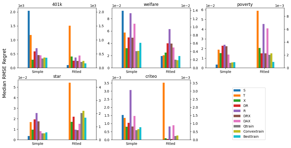
Figure 1: Median RMSE Regret for Each DGP.

For simple CATE functions, Table 2 shows that there is an decrease in the mean and median RMSE regret for Q-aggregation, when compared with convex stacking and model selection for every dataset. For datesets generated with the fitted CATE functions, the underlying model follows a S-learner setup. Thus, we expect the S-learners to be dominant models, which is evident Table 1. As a result, we observe that the there is often an increase in the RMSE regret for ensemble models over the best single model, as is hinted by Theorem 1, since in this case we have a dominant model.

 

Causal Q-Aggregation for CATE Model Selection: Appendix

 

Contents

1. 1 Introduction
2. 2 Preliminaries
3. 3 ERM-Based Selection
4. 4 Q-Aggregation with Nuisances
   1. 4.1 Square Losses with Nuisance Functions
   2. 4.2 Connections to Neyman Orthogonality
5. 5 Doubly Robust Q-Aggregation
6. 6 Doubly Robust Q-Aggregation for CATE with Instruments
7. 7 Experiments
8. A Detailed Comparison with Prior Works
   1. A.1 Comparison to Van Der Laan and Dudoit, (2003)
9. B Proofs for ERM-Based Selection
   1. B.1 Preliminaries
   2. B.2 Best-ERM: Proof of Theorem 1 of the Main Paper
   3. B.3 Convex-ERM: Proof of Theorem 2 of the Main Paper
10. C Mixed Bias Properties
    1. C.1 Doubly Robust Targets for CATE under Conditional Exogeneity
    2. C.2 Doubly Robust Targets for CATE with Instruments
11. D Experiment Details
    1. D.1 Candidate Models
    2. D.2 Data Generating Processes for Synthetic Datasets
    3. D.3 Semi-synthetic Datasets
    4. D.4 Additional Results
12. E Proof of Main Theorem
    1. E.1 Concentration of offset empirical processes
    2. E.2 Putting it all together
    3. E.3 Basic concentration proofs
    4. E.4 Auxiliary Lemmas
13. F Proof of Corollaries for Square Losses
    1. F.1 Relaxed Nuisance Guarantees Under Eigenvalue Condition
14. G Proof of Main Theorem without Sample Splitting
    1. G.1 Putting it all together
15. H Greedy Q-aggregation for Square Losses
    1. H.1 Preliminaries
    2. H.2 Excess Risk Guarantees for the k-step Greedy Q-aggregation Estimator
16. I Proof of Orthogonal Statistical Learning Theorem
    1. I.1 Fast Rates
    2. I.2 Slow Rates
       1. I.2.1 With Universal Orthogonality
       2. I.2.2 Without Universal Orthogonality

Appendix A Detailed Comparison with Prior Works

In traditional supervised learning, the standard approach for model selection is through M-fold cross validation, also called the discrete super learner. Vaart et al., (2006) proved an oracle inequality (under conditions):

$$\mathbb{E}[R(\hat{f})]-\mathbb{E}[R(f^{*})]\leq O\left(\mathbb{E}[R(f^{*})]+\frac{\log(M)}{n}\right)$$ (70)

where $\hat{f}$ is the best model selected by K-fold cross validation, $f^{*}$ is the oracle model selection, and $R(f)$ is the excess risk. Similar oracle inequalities are also provided in Van der Laan et al., (2007). Moreover, Van Der Laan and Dudoit, (2003) proved similar oracle inequalities for cross-validation even in the presence of nuisance functions in the loss. Our results on ERM-based selection and Q-aggregation based selection improve upon the results of Van Der Laan and Dudoit, (2003) on many critical directions. In summary, the results in Van Der Laan and Dudoit, (2003) cannot yield the doubly robust form of the dependence in the errors of the nuisances, for our main application to CATE model selection. Moreover, the selection rate results in Van Der Laan and Dudoit, (2003) depend on the performance of the best model in the set and only provide slow rates if the loss of the best model is not close to zero. Given the subtleties of the comparison of the results in Van Der Laan and Dudoit, (2003) and our work, we give very detailed comparison in the next subsection.

A similar oracle inequality was shown when ERM is used for model selection (Mitchell and van de Geer,, 2009). In addition, under strong assumptions on the tails of the centered excess losses, the authors proved that model selection via ERM can achieve a tail bound that with probability $1-\delta$:

$$R(\hat{f})-R(f^{*})\leq O\left(R(f^{*})+\frac{\log(M)}{n}+\frac{\log(1/\delta)}{n}\right)$$ (71)

Model Selection is particularly difficult for CATE estimation due to the lack of ground truth counterfactual data, making it difficult to evaluate model performance. Existing model selection criterion include the influence corrected loss (Alaa and Van Der Schaar,, 2019), R-loss for double machine learning (Nie and Wager,, 2021), doubly robust loss (Saito and Yasui,, 2020), the X-score (Künzel et al.,, 2019), matching score, (Rolling and Yang,, 2014), calibration score (Dwivedi et al.,, 2020), etc. In two recently conducted benchmarking studies on model selection for CATE estimators (Mahajan et al.,, 2022; Curth and van der Schaar,, 2023), the results showed that no single evaluation metric stood out as the dominant choice. Moreover, Mahajan et al., (2022) demonstrated that softmax stacking of the estimators often lead to better performance for any proxy evaluation metric.

Another line of work employs stacking which optimizes model weights by minimizing some performance metric on a held-out sample. Grimmer et al., (2017) constructed a weighted average across different potential outcome models via a cross validation based super learning approach(Van der Laan et al.,, 2007) that estimates the weights from out-of-sample performance through regression. In contrast to our work, Grimmer et al., (2017) applies stacking to the nuisance function that is used to construct the estimator, instead of the estimator itself. Closer to our line of work, Nie and Wager, (2021) proposed to use a positive linear combination of different estimators that minimizes their proposed R-loss on a validation sample. Although both work demonstrated empirical success, they did not provide any theoretical guarantees for stacking.

Bridging this gap, Han and Wu, (2022) studied the the theoretical guarantees of their proposed stacking algorithm when compared to oracle model selection. The proposed causal stacking algorithm learns a convex combination of the candidate models by optimizing the doubly robust loss on a validation set. Notably, what we are presenting in this work, that is Q aggregation, can be reduced to causal stacking when choose the same loss and some hyperparameter is set to 0. Han and Wu showed that, with probability $1-\delta$, the RMSE regret is on the order of $\sqrt{\frac{\log(M^{2})/\delta}{n}}$, which is a slower rate that what we presented in this paper. Interestingly, allowing the weights to be any non-negative value instead of summing to 1 improved performance when the treatment assignment is balanced.

More recently, Sugasawa et al., (2023) sought a different approach to construct ensembles which uses the Bayesian predictive synthesis(McAlinn and West,, 2019) framework, which allows the model/posterior weights to depend on the covariates, enabling the final ensemble to capture the heterogeneity of the performance of different models.

In our work, we provide additional theoretical results utilizing the orthogonal statistical learning framework (Foster and Syrgkanis,, 2023) when a Neyman orthogonal loss (e.g. the doubly robust loss) is used. In Section 3, we present results for both model selection and convex stacking using plug-in empirical risk minimization. In addition, we propose Q-aggregation (Lecué and Rigollet,, 2014) for CATE estimation, which constructs a convex combination of the candidate functions via a modified version of empirical risk minimization, and achieves optimal rate (Tsybakov,, 2003) of $O(\frac{\log(M)}{n})$ plus higher order error terms for the nuisance functions.

A.1 Comparison to Van Der Laan and Dudoit, (2003)

Van Der Laan and Dudoit, (2003) proved oracle inequalities for cross-validation that considers the need to estimate nuisance functions for the loss function. Here, we reproduce the main theorem in Van Der Laan and Dudoit, (2003) using our notation.

Theorem 9 (Theorem 1 of Van Der Laan and Dudoit, (2003)).

Let $f_{\hat{k}}$ and $f_{\tilde{k}}$ denote the best model selected by cross-validation and oracle model selection respectively. Define the excess risk with respect to the true candidate model as $d(f,f_{0})=\mathbb{E}_{S_{n}}[P(\ell_{f,g_{0}}-\ell_{f_{0},g_{0}})]$, where $S_{n}$ is the data split. Let $p$ denote the proportion of data used for validation in each split. Further define:

$$r_{1}(n)=~{} \max_{\bar{k}\in\{\hat{k},\tilde{k}\}}\frac{\mathbb{E}\left[P(\ell_{f_{\bar{k}},\hat{g}}-\ell_{f_{0},\hat{g}})-P(\ell_{f_{\bar{k}},g_{0}}-\ell_{f_{0},g_{0}})\right]}{\sqrt{\mathbb{E}[P(\ell_{f_{\bar{k}},g_{0}}-\ell_{f_{0},g_{0}})]}}$$ (72)

$$r_{2}(n)=~{} \mathbb{E}\left[\max_{k}\sqrt{P\left((\ell_{f_{k},\hat{g}}-\ell_{f_{0},\hat{g}})-(\ell_{f_{k},g_{0}}-\ell_{f_{0},g_{0}})\right)^{2}}\right]$$ (73)

$$\tilde{r}(n)=~{} \sqrt{\mathbb{E}[d(f_{\tilde{k}},f_{0})]}$$ (74)

Assuming that the nuisance estimator $\hat{g}$ converges to the true nuisance function $g_{0}$ as $n\rightarrow\infty$, the loss function is uniformly bounded by some constant $M_{1}$ for any $f\in F$, and $Var(\ell_{f,g_{0}}-\ell_{f_{0},g_{0}})\leq M_{2}\mathbb{E}[\ell_{f,g_{0}}-\ell_{f_{0},g_{0}}]$ for some constant $M_{2}$, then for any $\delta>0$:

$$\sqrt{\mathbb{E}[d(f_{\hat{k}},f_{0})]}\leq\frac{(1+\delta)r_{1}(n)+\sqrt{(1+\delta)^{2}r_{1}(n)^{2}+4\epsilon_{n}(\delta)}}{2}=:\sqrt{R(n)}$$ (75)

where

$$\epsilon_{n}(\delta)=~{} (1+2\delta)\tilde{r}^{2}(n)+4(1+\delta)^{2}\left(\frac{2M_{1}}{3}+\frac{M_{2}}{\delta}\right)\frac{1+\log(M)}{np}+$$ (76)

$$(1+\delta)r_{1}(n)\tilde{r}(n)+\frac{2M_{3}(1+\delta)\log(M)}{(np)^{0.5}}\max\left(r_{2}(n),(np)^{-0.5}I\left(r_{2}(n)>0\right)\right)$$ (77)

And $M_{3}$ is given by:

$$M_{3}(n)=\frac{M_{1}}{3}+\sqrt{2}\frac{\sqrt{\log(2)}}{\log(M)}+\frac{\sqrt{2}}{\sqrt{\log(M)}}+b_{0}+\int_{b_{0}}^{\infty}2M^{1-m(x)}dx$$ (78)

where

$$m(x)=\frac{1}{2}\frac{x^{2}}{1/\log(M)+\frac{4}{3M_{1}}x}$$ (79)

and $b_{0}$ is the solution to $1-m(x)=0$.

Note that $1-m(x)$ is decreasing in $x$. Thus $M_{3}(n)$ is upper and lower bounded by some strictly positive constant factor that only depends on $M_{1}$. Up to a constant factor $C(M_{1},M_{2})$ that depends only on $M_{1},M_{2}$ (and assuming for simplification that $\delta\leq 1$), the above can be simplified as:

$$R(n)\sim~{} (1+\delta)^{2}r_{1}(n)^{2}+4\epsilon_{n}(\delta)$$ (81)

$$\sim~{} (1+2\delta)\mathbb{E}[d(f_{\tilde{k}},f_{0})]+C(M_{1},M_{2})\left(\frac{1}{\delta}\frac{\log(M)}{n}+r_{1}(n)^{2}+r_{1}(n)\,\tilde{r}(n)+\frac{\log(M)}{\sqrt{n}}r_{2}(n)\right)$$ (82)

Thus this upper bound, provides selection rates of the form:

$$\mathbb{E}[d(f_{\hat{k}},f_{0})]-\mathbb{E}[d(f_{\tilde{k}},f_{0})]\lesssim 2\delta\mathbb{E}[d(f_{\tilde{k}},f_{0})]+C(M_{1},M_{2})\left(\frac{1}{\delta}\frac{\log(M)}{n}+r_{1}(n)^{2}+r_{1}(n)\,\tilde{r}(n)+\frac{\log(M)}{\sqrt{n}}r_{2}(n)\right)$$ (83)

As a side note, if we assume that the true nuisance parameter is known, i.e. $g_{0}$ is known, then $r_{1}(n)=r_{2}(n)=0$, and we get the same type of results as in Van der Laan et al., (2007).

Invoking the theorem with the square loss that we used in our paper, we get:

$$d(f,f_{0}):=~{} \|f-f_{0}\|^{2}$$ (84)

$$r_{1}(n)^{2}=~{} \Theta\left(\frac{\mathbb{E}\left[\textsc{Bias}(X;\hat{g})\,(f_{\bar{k}}(X)-f_{0}(X))\right]^{2}}{\mathbb{E}\left[\|f_{\bar{k}}-f_{0}\|^{2}\right]}\right)\stackrel{{\scriptstyle(i)}}{{\leq}}\Theta\left(\frac{\mathbb{E}\left[\textsc{Bias}(X;\hat{g})^{2}\right]\,\mathbb{E}\left[(f_{\bar{k}}(X)-f_{0}(X))^{2}\right]}{\mathbb{E}\left[\|f_{\bar{k}}-f_{0}\|^{2}\right]}\right)$$ (85)

$$=~{} \Theta\left(\frac{\mathbb{E}\left[\textsc{Bias}(X;\hat{g})^{2}\right]\mathbb{E}[\|f_{\bar{k}}-f_{0}\|^{2}]}{\mathbb{E}\left[\|f_{\bar{k}}-f_{0}\|^{2}\right]}\right)=\Theta(\mathbb{E}\left[\textsc{Bias}(X;\hat{g})^{2}\right])$$ (86)

$$r_{2}(n)^{2}=~{} \mathbb{E}\left[\max_{j}\left\{\mathbb{E}\left[\mathbb{E}[(\hat{Y}(\hat{g})-\hat{Y}(g_{0}))^{2}|X](f_{j}(X)-f_{0}(X))^{2}\right]\right\}\right]=\Theta\left(\mathbb{E}\left[(\hat{Y}(\hat{g})-\hat{Y}(g_{0}))^{2}\right]\right)$$ (87)

$$f_{*}:=~{} f_{\tilde{k}},~{}~{}~{}\tau_{0}:=f_{0},~{}~{}~{}~{}\hat{f}:=f_{\hat{k}}$$ (88)

$$\tilde{r}(n)=~{} \|f_{*}-\tau_{0}\|^{2}$$ (89)

Moreover, inequality $(i)$ is tight whenever $\textsc{Bias}(X;\hat{g})$ is independent of $f_{k}(X)-f_{0}(X)$, which cannot be excluded without further hard-to-justify assumptions. Therefore, the result of Van Der Laan and Dudoit, (2003) yields bounds of the form:

$${\cal S}(n):=~{} \|\hat{f}-\tau_{0}\|^{2}-\|f_{*}-\tau_{0}\|^{2}$$ (90)

$$\leq~{} \Theta\left(\delta\|f_{*}-\tau_{0}\|^{2}+\frac{1}{\delta}\frac{\log(M)}{n}+\mathbb{E}\left[\textsc{Bias}(X;\hat{g})^{2}\right]+\sqrt{\mathbb{E}\left[\textsc{Bias}(X;\hat{g})^{2}\right]}\|f_{*}-\tau_{0}\|+{\frac{\log(M)}{\sqrt{n}}}\mathbb{E}\left[(\hat{Y}(\hat{g})-\hat{Y}(g_{0}))^{2}\right]^{{\frac{1}{2}}}\right)$$ (91)

for any constant $\delta>0$. Note that the optimal choice of $\delta$, yields a rate of:

$${\cal S}(n)\leq~{} \Theta\left(\|f_{*}-\tau_{0}\|\,\sqrt{\frac{\log(M)}{n}}+\mathbb{E}\left[\textsc{Bias}(X;\hat{g})^{2}\right]+\sqrt{\mathbb{E}\left[\textsc{Bias}(X;\hat{g})^{2}\right]}\|f_{*}-\tau_{0}\|+{\frac{\log(M)}{\sqrt{n}}}\mathbb{E}\left[(\hat{Y}(\hat{g})-\hat{Y}(g_{0}))^{2}\right]^{{\frac{1}{2}}}\right)$$ (92)

On the contrary, our Theorem 1 yields an oracle inequality of the form:

$${\cal S}(n)\leq~{} O\left(\epsilon+\frac{\log(M)}{n}+\mathbb{E}\left[\textsc{Bias}(X;\hat{g})^{2}\right]\right) \epsilon=~{} \|f_{*}-\tau_{0}\|^{2}-\|\bar{f}_{*}-\tau_{0}\|^{2}$$ (93)

We identify the following critical differences in the two results:

1. The term ${\frac{\log(M)}{\sqrt{n}}}\mathbb{E}\left[(\hat{Y}(\hat{g})-\hat{Y}(g_{0}))^{2}\right]^{{\frac{1}{2}}}$ that appears in the result of Van Der Laan and Dudoit, (2003) does not appear in our bound. This is crucial for the doubly robust application. Note that $\mathbb{E}[\textsc{Bias}(X;\hat{g})^{2}]$ takes the form of the product of the errors of the propensity and the regression estimates, i.e. $\mathbb{E}[(\hat{\alpha}-\alpha_{0})^{2}\,(\hat{g}-g_{0})^{2}]$. On the contrary the quantity $\mathbb{E}\left[(\hat{Y}(\hat{g})-\hat{Y}(g_{0}))^{2}\right]^{{\frac{1}{2}}}$ does not take this product form. Thus, we would incur a dependence on the error of propensity and the regression, i.e. $\mathbb{E}[(\hat{\alpha}-\alpha_{0})^{2}]^{{\frac{1}{2}}}+\mathbb{E}[(\hat{g}-g_{0})^{2}]^{{\frac{1}{2}}}$. The latter wont converge faster than $1/{\sqrt{n}}$, even for parametric functions and thereby the estimation error of the regression and the propensity cannot be ignored in the selection error.

2. For any reasonable value of $\delta$, the result of Van Der Laan and Dudoit, (2003) would have a linear dependence on $\|f_{*}-\tau_{0}\|^{2}$. On the contrary our error only depends on the strictly smaller quanity $\epsilon=\|f_{*}-\tau_{0}\|^{2}-\|\bar{f}_{*}-\tau_{0}\|^{2}$, where $\bar{f}_{*}$ is the minizer of the square loss within the convex hull of the original set of functions. The quantity $\epsilon$ has the property that when there is a “dominant” model, such that the best in the convex hull puts almost all weight on one model, then $\epsilon$ is almost zero, while $\|f_{*}-\tau_{0}\|^{2}$ can be very far away from zero. Note that when $\|f_{*}-\tau_{0}\|$ is far from zero, then the optimal choice of $\delta$, yields only a slow rate of $\sqrt{\log(M)/n}$ and not a fast rate of $\log(M)/n$.

Moreover, our main Q-aggregation Theorem 3 yields an oracle inequality of the form:

$${\cal S}(n)\leq~{} O\left(\frac{\log(M)}{n}+\mathbb{E}\left[\textsc{Bias}(X;\hat{g})^{2}\right]\right)$$ (94)

We identify the following critical differences in the two results:

1. The term ${\frac{\log(M)}{\sqrt{n}}}\mathbb{E}\left[(\hat{Y}(\hat{g})-\hat{Y}(g_{0}))^{2}\right]^{{\frac{1}{2}}}$ does not appear in our bound, which is crucial for our doubly robust Q-aggregation results for the same reason as outlined in the bullet points above.

2. For any reasonable value of $\delta$, the result of Van Der Laan and Dudoit, (2003) would have a linear dependence on $\|f_{*}-\tau_{0}\|^{2}$. On the contrary our error bound incurs no dependence on the performance of the best model! Even if the best model is very far from the true function $f_{0}$, we still compete with the best model at a $\log(M)/n+\mathbb{E}[\textsc{Bias}(X;\hat{g})^{2}]$ rate.

Appendix B Proofs for ERM-Based Selection

B.1 Preliminaries

We will be invoking a generalization of orthogonal statistical learning theorem (Foster and Syrgkanis,, 2023).

First, we describe the assumptions for the theorem. Let $F$ and $F^{\prime}$ be two function spaces such that $F\subseteq F^{\prime}$. Consider $f_{*}\in F$ and $f^{\prime}\in F^{\prime}$. Let $d(g,g_{0})$ denote a distance metric in the function space $G$. The the remaining of the section, we will assume that the loss $\ell_{f,g}$ is $C_{b}$-lipschitz in $f(X)$.

ASSUMPTION 1 (Orthogonal Loss).

The population risk is Neyman Orthogonal, i.e. for all $\bar{f}\in\text{Star}(F,f^{\prime})$ and $g\in G$:

$$D_{f}D_{g}P\ell_{f^{\prime},g_{0}}(Z)[g-g_{0},f-f^{\prime}]=0$$ (95)

ASSUMPTION 2 (First Order Optimality).

The estimator $f^{\prime}$ for the population risk satisfies the first-order optimality condition:

$$D_{f}P\ell_{f^{\prime},g_{0}}(Z)[f-f^{\prime}]\geq 0\quad\forall f\in\text{Star}(F,f^{\prime})$$ (96)

ASSUMPTION 3 (Higher Order Smoothness).

There exist constants $\beta_{1}$ and $\beta_{2}$ such that the following holds:

• Second order smoothness with respect to the target $f$. For all $f\in F$ and all $\bar{f}\in\text{Star}(F,f^{\prime})$:

  $$D^{2}_{f}P\ell_{\bar{f},g_{0}}(Z)[f-f^{\prime},f-f^{\prime}]\leq\beta_{1}\|f-f^{\prime}\|^{2}$$ (97)

• Higher order smoothness. There exist $r\in[0,1)$ such that for all $f\in\text{Star}(F,f^{\prime})$, $g\in G$, and $\bar{g}\in\text{Star}(G,g_{0})$:

  $$\left|D^{2}_{g}D_{f}P\ell_{f^{\prime},\bar{g}}(Z)[f-f^{\prime},g-g_{0},g-g_{0}]\right|\leq\beta_{2}\|f-f^{\prime}\|^{1-r}d(g,g_{0})^{2}$$ (98)

ASSUMPTION 4 (Strong Convexity).

The population risk is strongly convex with respect to the target function: there exist constants $\lambda$, $\kappa>0$ such that for all $f\in F$ and an estimate $\hat{g}\in G$.

$$D^{2}_{f}P\ell_{\bar{f},\hat{g}}(Z)[f-f^{\prime},f-f^{\prime}]\geq\lambda\|f-f^{\prime}\|^{2}-\kappa d(\hat{g},g_{0})^{\frac{4}{1+r}}\quad\forall\bar{f}\in\text{Star}(F,f^{\prime})$$ (99)

Alternatively, Assumption 1 and Assumption 3(b) may be replaced by the following assumption.

ASSUMPTION 5.

There exist $r\in[0,1)$ and constant $\beta_{3}$ such that for all $f,\bar{f}\in\text{Star}(F,f^{\prime})$, $g\in G$:

$$|D_{f}P\ell(\bar{f},g)[f-f^{\prime}]-D_{f}P\ell(\bar{f},g_{0})[f-f^{\prime}]|\leq\beta_{3}\|f-f^{\prime}\|^{1-r}d(g,g_{0})^{2}$$ (100)

Theorem 10 (Fast Rates Under Strong Convexity (Foster and Syrgkanis,, 2023)).

Suppose Assumptions 1 to 4, or alternatively, Assumptions 2, 4, and 5 and Assumption 3(a), are satisfied for some $f^{\prime}\in F^{\prime}$ and function space $F\subseteq F^{\prime}$. Then any estimator $\hat{f}\in F$ satisfies:

$$P\ell_{\hat{f},g_{0}}(Z)-P\ell_{f^{\prime},g_{0}}(Z)\leq O\left(P\ell_{\hat{f},\hat{g}}(Z)-P\ell_{f^{\prime},\hat{g}}(Z)+d(\hat{g},g_{0})^{\frac{4}{1+r}}\right)$$ (101)

Moreover, if the estimator $\hat{f}$ satisfies with probability at least $1-\delta$,

$$P\ell_{\hat{f},\hat{g}}(Z)-P\ell_{f^{\prime},\hat{g}}(Z)\leq\epsilon_{n}(\delta)\|\hat{f}-f^{\prime}\|+\alpha_{n}(\delta)$$ (102)

for functions $\epsilon_{n}(\delta)$ and $\alpha_{n}(\delta)$, then we have, with probability at least $1-\delta$

$$P\ell_{\hat{f},g_{0}}(Z)-P\ell_{f^{\prime},g_{0}}(Z)\leq O\left(\epsilon_{n}(\delta)^{2}+\alpha_{n}(\delta)+d(\hat{g},g_{0})^{\frac{4}{1+r}}\right)$$ (103)

Despite the small generalization made to consider any $f^{\prime}\in F^{\prime}$ that satisfies the first order optimality condition, the proof follows the original proof closely, and is included in Section I for completeness. We also showed that the same results can be obtained if Assumption 5 is satisfied instead of Assumptions 1 and 3.

Lemma 11.

Assume that the Assumptions 1 and 3(b) hold, or alternatively Assumption 5 holds, for some $f^{\prime}\in F^{\prime}$. Then for any $f_{*}\in F$ we have:

$$P\ell_{\hat{f},\hat{g}}(Z)-P\ell_{f^{\prime},\hat{g}}(Z)\leq P\ell_{\hat{f},\hat{g}}(Z)-P\ell_{f_{*},\hat{g}}(Z)+{2(P\ell_{f_{*},g_{0}}(Z)-P\ell_{f^{\prime},g_{0}}(Z))+O\left(((2/\lambda)^{\frac{2}{1+r}}+\kappa)\,d(\hat{g},g_{0})^{\frac{4}{1+r}}\right)}$$ (104)

Moreover, if $\ell$ is a square loss, we have:

$$P\ell_{\hat{f},\hat{g}}(Z)-P\ell_{f^{\prime},\hat{g}}(Z)\leq P\ell_{\hat{f},\hat{g}}(Z)-P\ell_{f_{*},\hat{g}}(Z)+{2\left(\|f_{*}-\tau_{0}\|^{2}-\|f^{\prime}-\tau_{0}\|^{2}\right)+O\left(d(\hat{g},g_{0})^{\frac{4}{1+r}}\right)}$$ (105)

Proof.

$$P\ell_{\hat{f},\hat{g}}(Z)-P\ell_{f^{\prime},\hat{g}}(Z)=~{} (P\ell_{\hat{f},\hat{g}}(Z)-P\ell_{f_{*},\hat{g}}(Z))+(P\ell_{f_{*},\hat{g}}(Z)-P\ell_{f^{\prime},\hat{g}}(Z))$$ (106)

Let us first consider the case where Assumptions 1 and 3(b) holds. For any $g$, taking a first order Taylor expansion yields:

$$P\ell_{f_{*},g}(Z)-P\ell_{f^{\prime},g}(Z)=D_{f}P\ell_{\bar{f},g}(Z)[f_{*}-f^{\prime}]$$ (107)

for some $\bar{f}\in\text{Star}(F,f^{\prime})$. Let us first consider the excess risk for evaluated at $g_{0}$.

Taking a second order Taylor expansion for the $(P\ell_{f_{*},\hat{g}}(Z)-P\ell_{f^{\prime},\hat{g}}(Z))$ term at $g_{0}$, we get:

$$(P\ell_{f_{*},\hat{g}}(Z)-P\ell_{f^{\prime},\hat{g}}(Z))=~{} (P\ell_{f_{*},g_{0}}(Z)-P\ell_{f^{\prime},g_{0}}(Z))+D_{g}D_{f}P\ell_{\bar{f},g_{0}}(Z)[f_{*}-f^{\prime},\hat{g}-g_{0}]$$ (108)

$$+~{} \frac{1}{2}D_{g}^{2}D_{f}P\ell_{\bar{f},\bar{g}}(Z)[f_{*}-f^{\prime},\hat{g}-g_{0},\hat{g}-g_{0}]$$ (109)

$$=~{} (P\ell_{f_{*},g_{0}}(Z)-P\ell_{f^{\prime},g_{0}}(Z))+\frac{1}{2}D_{g}^{2}D_{f}P\ell_{\bar{f},\bar{g}}(Z)[f_{*}-f^{\prime},\hat{g}-g_{0},\hat{g}-g_{0}]$$ (By Assumption 1)

$$\leq~{} (P\ell_{f_{*},g_{0}}(Z)-P\ell_{f^{\prime},g_{0}}(Z))+\frac{1}{2}D_{g}^{2}D_{f}P\ell_{\bar{f},\bar{g}}(Z)[f_{*}-f^{\prime},\hat{g}-g_{0},\hat{g}-g_{0}]$$ (110)

$$\leq~{} (P\ell_{f_{*},g_{0}}(Z)-P\ell_{f^{\prime},g_{0}}(Z))+\frac{\beta_{2}}{2}\|f_{*}-f^{\prime}\|^{1-r}d(\hat{g},g_{0})^{2}$$ (By Assumption 3(b))

$$\leq~{} (P\ell_{f_{*},g_{0}}(Z)-P\ell_{f^{\prime},g_{0}}(Z)){+\frac{\lambda}{2}\|f_{*}-f^{\prime}\|^{2}+O\left((2/\lambda)^{\frac{2}{1+r}}d(\hat{g},g_{0})^{\frac{4}{1+r}}\right)}$$ (Young’s inequality)

Alternatively, if Assumption 5 holds, then it follows immediately from a first order Taylor expansion that

$$(P\ell_{f_{*},\hat{g}}(Z)-P\ell_{f^{\prime},\hat{g}}(Z))-(P\ell_{f_{*},g_{0}}(Z)-P\ell_{f^{\prime},g_{0}}(Z))=~{} D_{f}P\ell(\bar{f},g)[\hat{f}-f^{\prime}]-D_{f}P\ell(\bar{f},g_{0})[\hat{f}-f^{\prime}]$$ (111)

$$\leq~{} \beta_{3}\|f-f^{\prime}\|^{1-r}d(\hat{g},g_{0})^{2}$$ (112)

$$\leq~{} {\frac{\lambda}{2}\|f_{*}-f^{\prime}\|^{2}+O\left((2/\lambda)^{\frac{2}{1+r}}d(\hat{g},g_{0})^{\frac{4}{1+r}}\right)}$$ (113)

and the same result follows.

By the first order optimality of $f^{\prime}$ and strong convexity, we have that:

$$P\ell_{f_{*},g_{0}}(Z)-P\ell_{f^{\prime},g_{0}}(Z)\geq D_{f}P\ell_{f^{\prime},g_{0}}[f_{*}-f^{\prime}]+\frac{\lambda}{2}\|f_{*}-f^{\prime}\|^{2}-\frac{\kappa}{2}d(\hat{g},g_{0})^{\frac{4}{1+r}}\geq\frac{\lambda}{2}\|f_{*}-f^{\prime}\|^{2}-\frac{\kappa}{2}d(\hat{g},g_{0})^{\frac{4}{1+r}}$$ (114)

Thus we deduce that:

$$P\ell_{f_{*},\hat{g}}(Z)-P\ell_{f^{\prime},\hat{g}}(Z)\leq 2(P\ell_{f_{*},g_{0}}(Z)-P\ell_{f^{\prime},g_{0}}(Z))+O\left(((2/\lambda)^{\frac{2}{1+r}}+\kappa)d(\hat{g},g_{0})^{\frac{4}{1+r}}\right)$$ (115)

For square losses, $\lambda=2$, $\kappa=0$ and as we will show in Section F (by the realizability of $\tau_{0}$, i.e. $\mathbb{E}[Y(g_{0})\mid X]=\tau_{0}(X)$):

$$(P\ell_{f_{*},g_{0}}(Z)-P\ell_{f^{\prime},g_{0}}(Z))=\|f_{*}-\tau_{0}\|^{2}-\|f^{\prime}-\tau_{0}\|^{2}$$ (116)

So we get:

$$P\ell_{\hat{f},\hat{g}}(Z)-P\ell_{f^{\prime},\hat{g}}(Z)\leq~{} (P\ell_{\hat{f},\hat{g}}(Z)-P\ell_{f_{*},\hat{g}}(Z))+2(\|f_{*}-\tau_{0}\|^{2}-\|f^{\prime}-\tau_{0}\|^{2})+O\left(d(\hat{g},g_{0})^{\frac{4}{1+r}}\right)$$ (117)

∎

Corollary 12 (Generalization of Theorem 10).

Suppose Assumptions 1 to 4, or alternatively, Assumptions 2, 4, and 5 and Assumption 3(a), are satisfied for some $f^{\prime}\in F^{\prime}$ and function space $F\subseteq F^{\prime}$ and for some constants $\lambda,\beta_{1},\beta_{2},\beta_{3},\kappa,r$. Let $f_{*}$ be any function in $F$. Then any estimator $\hat{f}\in F$ satisfies

$$P\ell_{\hat{f},g_{0}}(Z)-P\ell_{f^{\prime},g_{0}}(Z)\leq O\left(P\ell_{\hat{f},\hat{g}}(Z)-P\ell_{f_{*},\hat{g}}(Z)+(P\ell_{f_{*},g_{0}}(Z)-P\ell_{f^{\prime},g_{0}}(Z))+d(\hat{g},g_{0})^{\frac{4}{1+r}}\right)$$ (118)

and for square losses:

$$P\ell_{\hat{f},g_{0}}(Z)-P\ell_{f^{\prime},g_{0}}(Z)\leq O\left(P\ell_{\hat{f},\hat{g}}(Z)-P\ell_{f_{*},\hat{g}}(Z)+\|f_{*}-\tau_{0}\|^{2}-\|f^{\prime}-\tau_{0}\|^{2}+d(\hat{g},g_{0})^{\frac{4}{1+r}}\right)$$ (119)

Moreover, if the estimator $\hat{f}$ satisfies w.p. $1-\delta$

$$P\ell_{\hat{f},\hat{g}}(Z)-P\ell_{f_{*},\hat{g}}(Z)\leq\epsilon_{n}(\delta)\|\hat{f}-f_{*}\|+\alpha_{n}(\delta)$$ (120)

for functions $\epsilon_{n}(\delta)$ and $\alpha_{n}(\delta)$, then we have, with probability at least $1-\delta$

$$P\ell_{\hat{f},g_{0}}(Z)-P\ell_{f^{\prime},g_{0}}(Z)\leq O\left((P\ell_{f_{*},g_{0}}(Z)-P\ell_{f^{\prime},g_{0}}(Z))+\epsilon_{n}(\delta)^{2}+\alpha_{n}(\delta)+d(\hat{g},g_{0})^{\frac{4}{1+r}}\right)$$ (121)

and for square losses:

$$P\ell_{\hat{f},g_{0}}(Z)-P\ell_{f^{\prime},g_{0}}(Z)\leq O\left(\|f_{*}-\tau_{0}\|^{2}-\|f^{\prime}-\tau_{0}\|^{2}+\epsilon_{n}(\delta)^{2}+\alpha_{n}(\delta)+d(\hat{g},g_{0})^{\frac{4}{1+r}}\right)$$ (122)

Proof.

The first result follows from a direct application of Lemma 11.

Next,

$$P\ell_{\hat{f},\hat{g}}(Z)-P\ell_{f_{*},\hat{g}}(Z)\leq~{} \epsilon_{n}(\delta)\|\hat{f}-f_{*}\|+\alpha_{n}(\delta)$$ (123)

$$\leq~{} \epsilon_{n}(\delta)(\|\hat{f}-f^{\prime}\|+\|f_{*}-f^{\prime}\|)+\alpha_{n}(\delta)$$ (124)

$$\leq~{} \epsilon_{n}(\delta)\|\hat{f}-f^{\prime}\|+\frac{1}{2}\epsilon_{n}(\delta)^{2}+\frac{1}{2}\|f_{*}-f^{\prime}\|^{2}+\alpha_{n}(\delta)$$ (125)

By the first order optimality of $f^{\prime}$ and strong convexity, we have that:

$$P\ell_{f_{*},g_{0}}(Z)-P\ell_{f^{\prime},g_{0}}(Z)\geq D_{f}P\ell_{f^{\prime},g_{0}}[f_{*}-f^{\prime}]+\lambda\|f_{*}-f^{\prime}\|^{2}-\kappa d(g,g_{0})^{\frac{4}{1+r}}\geq\lambda\|f_{*}-f^{\prime}\|^{2}-\kappa d(\hat{g},g_{0})^{\frac{4}{1+r}}$$ (126)

Thus:

$$P\ell_{\hat{f},\hat{g}}(Z)-P\ell_{f_{*},\hat{g}}(Z)\leq~{} \epsilon_{n}(\delta)\|\hat{f}-f^{\prime}\|+\frac{1}{2}\epsilon_{n}(\delta)^{2}+\alpha_{n}(\delta)+O\left(P\ell_{f_{*},g_{0}}(Z)-P\ell_{f^{\prime},g_{0}}(Z)+d(\hat{g},g_{0})^{\frac{4}{1+r}}\right)$$ (127)

Applying Lemma 11 yields:

$$P\ell_{\hat{f},\hat{g}}(Z)-P\ell_{f^{\prime},\hat{g}}(Z)\leq~{} (P\ell_{\hat{f},\hat{g}}(Z)-P\ell_{f_{*},\hat{g}}(Z))+O\left((P\ell_{f_{*},g_{0}}(Z)-P\ell_{f^{\prime},g_{0}}(Z))+d(\hat{g},g_{0})^{\frac{4}{1+r}}\right)$$ (128)

$$\leq~{} \epsilon_{n}(\delta)\|\hat{f}-f^{\prime}\|+O\left(\epsilon_{n}(\delta)^{2}+\alpha_{n}(\delta)+(P\ell_{f_{*},g_{0}}(Z)-P\ell_{f^{\prime},g_{0}}(Z))+d(\hat{g},g_{0})^{\frac{4}{1+r}}\right)$$ (129)

Finally, invoking Theorem 10, we get:

$$P\ell_{\hat{f},g_{0}}(Z)-P\ell_{f^{\prime},g_{0}}(Z)\leq O\left(\epsilon_{n}(\delta)^{2}+\alpha_{n}(\delta)+(P\ell_{f_{*},g_{0}}(Z)-P\ell_{f^{\prime},g_{0}}(Z))+d(\hat{g},g_{0})^{\frac{4}{1+r}}\right)$$ (130)

Similarly for square losses. ∎

When strong convexity is not satisfied, slower oracle rates can be shown.

ASSUMPTION 6 (Universal Orthogonality).

For all $\bar{f}\in\text{Star}(F,f_{*})+\text{Star}(F-f_{*},0)$,

$$D_{g}D_{f}P\ell_{\bar{f},g_{0}}(Z)[f-f_{*},g-g_{0}]=0\quad\forall g\in G,f\in F$$ (131)

ASSUMPTION 7.

The derivatives $D^{2}_{g}P\ell_{f,g}(Z)$ and $D^{2}_{f}D_{g}P\ell_{f,g}(Z)$ are continuous. Furthermore, there exists a constant $\beta$ such that for all $f\in\text{Star}(F,f_{*})$ and $\bar{g}\in\text{Star}(G,g_{0})$,

$$|D^{2}_{g}P\ell_{f,\bar{g}}[g-g_{0},g-g_{0}]|\leq\beta d(g,g_{0})^{2}\quad\forall g\in G$$ (132)

Similarly, Assumptions 6 to 7 can be replaced by the following assumption:

ASSUMPTION 8.

There exist a constant $\beta_{4}$ such that for all $f,\bar{f}\in\text{Star}(F,f^{\prime})$, $g\in G$:

$$|D_{f}P\ell(\bar{f},g)[f-f^{\prime}]-D_{f}P\ell(\bar{f},g_{0})[f-f^{\prime}]|\leq\beta_{4}d(g,g_{0})^{2}$$ (133)

Theorem 13 (Slow Rates without Strong Convexity).

Suppose that $f_{*}$ satisfies Assumptions 6 to 7, or alternatively, Assumption 8 holds, then with probability at least $1-\delta$, the target estimator $\hat{f}$ has the following exexss risk bound:

$$P\ell_{\hat{f},g_{0}}(Z)-P\ell_{f^{\prime},g_{0}}(Z)\leq O\left(P\ell_{\hat{f},\hat{g}}(Z)-P\ell_{f^{\prime},\hat{g}}(Z)+d(g,g_{0})^{2}\right)$$ (134)

B.2 Best-ERM: Proof of Theorem 1 of the Main Paper

First, we verify that Assumptions 2, 4, and 5 are satisfied for the square losses, so that Corollary 12 can be invoked.

Consider $f^{\prime}$ to be the minimizer of the population risk in the function space $F^{\prime}=\mathrm{co}(F)$. Since we can rewrite $\ell_{f,g_{0}}(Z)=\mathbb{E}[(f-\tau_{0})^{2}]+Var(\hat{Y}(g_{0}))$, it is straight forward to see that Assumption 2 is satisfied.

Moreover, for any function $g$, we have:

$$D^{2}_{f}P\ell_{\bar{f},g_{0}}(Z)[f-f^{\prime},f-f^{\prime}]=\mathbb{E}[2(f-f^{\prime})^{2}]=2\|f-f^{\prime}\|^{2}$$ (135)

Therefore, Assumption 4 are satisfied with $r=0$ and $\kappa=0$.

In Section F, we showed that:

$$|(P\ell_{f,g}(Z)-P\ell_{f^{\prime},g}(Z))-(P\ell_{f,g_{0}}(Z)-P\ell_{f^{\prime},g_{0}}(Z))|=2\sqrt{\mathbb{E}\left[\textsc{Bias}(\hat{g})]^{2}\right]}\,\|f_{\theta^{*}}-f_{\hat{\theta}}\|$$ (136)

Thus, Assumption 5 is satisfied with $r=0$, $\beta_{3}=2$, and $d(\hat{g},g_{0})=\mathbb{E}\left[\textsc{Bias}(\hat{g})]^{2}\right]^{\frac{1}{4}}$.

Next, we need to bound $P\ell_{\hat{f},\hat{g}}(Z)-P\ell_{f_{*},\hat{g}}(Z)$.

Invoking Lemma 14 from Foster and Syrgkanis, (2023), with probability at least $1-\delta$, we can bound the centered excess loss for ERM over any function class $F$ by:

$$(P-P_{n})({\ell}_{\hat{f},\hat{g}}(Z)-{\ell}_{f_{*},\hat{g}}(Z))\leq O\left(\delta_{n}\|\hat{f}-f_{*}\|+\delta_{n}^{2}\right)$$ (137)

where for any $f_{*}\in F$, $\delta_{n}=r_{n}+\sqrt{\frac{\log(1/\delta)}{n}}$, and $r_{n}$ is the critical radius of $\text{Star}(F-f_{*},0)$. In particular, we consider $f_{*}$ to be the minimizer of $\|f_{*}-f^{\prime}\|$ in $F$. By definition of $\hat{f}$, $P_{n}({\ell}_{\hat{f},\hat{g}}(Z)-{\ell}_{f_{*},\hat{g}}(Z))<0$, so we have:

$$P({\ell}_{\hat{f},\hat{g}}(Z)-{\ell}_{f_{*},\hat{g}}(Z))\leq(P-P_{n})({\ell}_{\hat{f},\hat{g}}(Z)-{\ell}_{f_{*},\hat{g}}(Z))\leq O\left(\delta_{n}\|\hat{f}-f_{*}\|+\delta_{n}^{2}\right)$$ (138)

As a result, we can instantiate Corollary 12 with $r=0$, and $d(\hat{g},g_{0})=\mathbb{E}\left[\textsc{Bias}(\hat{g})^{2}\right]^{\frac{1}{4}}$. Moreover, we can let $\epsilon_{n}=O(\delta_{n})$ and $\alpha_{n}=O(\delta_{n}^{2})$, to obtain:

$$\|\hat{f}-\tau_{0}\|^{2}-\|f^{\prime}-\tau_{0}\|^{2}=~{} P\ell_{\hat{f},g_{0}}(Z)-P\ell_{f^{\prime},g_{0}}(Z)$$ (139)

$$\leq~{} O\left(\delta_{n}^{2}+\|f_{*}-\tau_{0}\|^{2}-\|f^{\prime}-\tau_{0}\|^{2}+\mathbb{E}\left[\textsc{Bias}(\hat{g})^{2}\right]\right)$$ (140)

Applying the fact that, for $F=\{f_{1},f_{2},\dots,f_{M}\}$, the critical radius of the $\text{Star}(F-f_{*},0)$ is $r_{n}^{2}=\Theta\left(\frac{\log(\max\{M,n\})}{n}\right)$, we get:

$$\|\hat{f}-\tau_{0}\|^{2}-\|f^{\prime}-\tau_{0}\|^{2}\leq O\left(\frac{\log(\max\{M,n\}/\delta)}{n}+\|f_{*}-\tau_{0}\|^{2}-\|f^{\prime}-\tau_{0}\|^{2}+\mathbb{E}\left[\textsc{Bias}(\hat{g})^{2}\right]\right)$$ (141)

Since by definition, $f^{\prime}$ is equivalent to $\bar{f_{*}}$, we obtain a stronger result than in Theorem 1 in the main text, which bounds the regret with respect to the optimal convex combination of models instead of the best model:

$$\mathcal{S}(\hat{\theta})=~{} \|f_{\hat{\theta}}-\tau_{0}\|^{2}-\|f_{\theta_{*}}-\tau_{0}\|^{2}$$ (142)

$$\leq~{} \|f_{\hat{\theta}}-\tau_{0}\|^{2}-\|\bar{f_{\theta_{*}}}-\tau_{0}\|^{2}$$ (143)

$$\leq~{} O\left(\frac{\log(\max\{M,n\}/\delta)}{n}+\|f_{*}-\tau_{0}\|^{2}-\|f^{\prime}-\tau_{0}\|^{2}+\mathbb{E}\left[\textsc{Bias}(\hat{g})^{2}\right]\right)$$ (144)

B.3 Convex-ERM: Proof of Theorem 2 of the Main Paper

For ERM over the convex hull, we can follow the same arguments to invoke Theorem 10 with $r=0$, $\beta_{3}=2$, and $d(\hat{g},g_{0})=\mathbb{E}\left[\textsc{Bias}(\hat{g})]^{2}\right]^{\frac{1}{4}}$ as in the previous section, with $f_{*}=f^{\prime}=\bar{f_{*}}$ and $F^{\prime}=F=\mathrm{co}(\{f_{1},f_{2},\dots,f_{M}\})$, we get that:

$$\|\hat{f}-\tau_{0}\|^{2}-\|f_{*}-\tau_{0}\|^{2}\leq~{} O\left(\delta_{n}^{2}+\mathbb{E}\left[\textsc{Bias}(\hat{g})^{2}\right]\right)$$ (145)

By metric entropy arguments, the critical radius for this $\text{Star}(F-f_{*},0)$ is $r_{n}^{2}=\Theta\left(\sqrt{\frac{M\log(n)}{n}}\right)$. Combining, we get:

$$\|\hat{f}-\tau_{0}\|^{2}-\|f_{*}-\tau_{0}\|^{2}\leq~{} O\left(\frac{M\log(n/\delta)}{n}+\mathbb{E}\left[\textsc{Bias}(\hat{g})^{2}\right]\right)$$ (146)

On the other hand, a different nuisance error term can be obtained by invoking Theorem 13. First, we show that square losses satisfy Assumption 8. Assuming $f$ is uniformly bounded by $U$ for all $f\in F$, we have that:

$$|D_{f}P\ell(\bar{f},g)[f-f^{\prime}]-D_{f}P\ell(\bar{f},g_{0})[f-f^{\prime}]|=~{} |\mathbb{E}[(\bar{f}-\hat{Y}(g))(f-f^{\prime})-(\bar{f}-\hat{Y}(g_{0}))(f-f^{\prime})]|$$ (147)

$$=~{} |\mathbb{E}[(\hat{Y}(g)-\hat{Y}(g_{0}))(f-f^{\prime})]|$$ (148)

$$=~{} 2|\mathbb{E}[\textsc{Bias}(\hat{g})(\hat{f}-f^{\prime})]|$$ (149)

$$\leq~{} 4U\mathbb{E}[|\textsc{Bias}(\hat{g})|]$$ (150)

Thus, Assumption 8 is satisfied with $\beta_{4}=4U$ and $d(\hat{g},g_{0})=\mathbb{E}[|\textsc{Bias}(\hat{g})|]^{\frac{1}{2}}$.

Next, we need a generalization bound that does not involve $\|\hat{f}-f^{\prime}\|$ terms. With probability at least $1-\delta$:

$$(P-P_{n})(\ell_{\hat{f},\hat{g}}-\ell_{f^{\prime},\hat{g}})\leq~{} C_{b}(P-P_{n})(\hat{f}-f^{\prime}) \ell C_{b} f(X)$$ (Since we assume is Lipschitz in )

$$\leq~{} O\left(R(F)+\sqrt{\frac{\log(1/\delta)}{n}}\right)$$ (By standard generalization arguments)

where $R(F)$ is the Rademacher complexity of the function space $F$.

Thus invoking Theorem 13, we get:

$$\|\hat{f}-\tau_{0}\|^{2}-\|f_{*}-\tau_{0}\|^{2}\leq~{} O\left(R(F)+\sqrt{\frac{\log(1/\delta)}{n}}+\mathbb{E}\left[|\textsc{Bias}(\hat{g})|\right]\right)$$ (151)

$$\leq~{} O\left(\sqrt{\frac{\log(M)}{n}}+\sqrt{\frac{\log(1/\delta)}{n}}+\mathbb{E}\left[|\textsc{Bias}(\hat{g})|\right]\right)$$ (Lemma 26.11 in Shalev-Shwartz and Ben-David, (2014))

$$\leq~{} O\left(\sqrt{\frac{\log(M/\delta)}{n}}+\mathbb{E}\left[|\textsc{Bias}(\hat{g})|\right]\right)$$ (152)

As with the Best-ERM case, this bounds the regret with respect to the optimal convex combination of models instead of the best model, which is a stronger result than in Theorem 2 in the main text.

Appendix C Mixed Bias Properties

C.1 Doubly Robust Targets for CATE under Conditional Exogeneity

$$\mathbb{E}\left[\hat{Y}(g_{0})-\hat{Y}(\hat{g})\mid X\right]=~{} \mathbb{E}\left[a_{0}(D,W)\,h_{0}(D,W)\mid X\right]-\mathbb{E}\left[a_{0}(D,W)\,\hat{h}(D,W)\mid X\right]$$ (153)

$$~{}+\mathbb{E}\left[\hat{a}(D,W)\,(h_{0}(D,W)-\hat{h}(D,W))\mid X\right]$$ (154)

$$=~{} \mathbb{E}\left[(a_{0}(D,W)-\hat{a}(D,W))\,(h_{0}(D,W)-\hat{h}(D,W))\mid X\right]$$ (155)

$$=~{} \mathbb{E}\left[\hat{q}(D,W)\mid X\right]$$ (156)

C.2 Doubly Robust Targets for CATE with Instruments

$$\mathbb{E}[\hat{Y}(\hat{g})-\hat{Y}(g_{0})\mid X]=~{} \hat{\tau}(X)+\frac{\mathbb{E}[Y\tilde{Z}\mid X]-\hat{\tau}(X)\mathbb{E}[D\tilde{Z}\mid X]}{\hat{\beta}(X)}-\tau_{0}(X)$$ (157)

$$=~{} \hat{\tau}(X)+\frac{\tau_{0}(X)\beta_{0}(X)-\hat{\tau}(X)\beta_{0}(X)}{\hat{\beta}(X)}-\tau_{0}(X)$$ (158)

$$=~{} \hat{\tau}(X)-\tau_{0}(X)+(\tau_{0}(X)-\hat{\tau}(X))\frac{\beta_{0}(X)}{\hat{\beta}(X)}$$ (159)

$$=~{} (\tau_{0}(X)-\hat{\tau}(X))\left(\frac{\beta_{0}(X)}{\hat{\beta}(X)}-1\right)$$ (160)

$$=~{} (\tau_{0}(X)-\hat{\tau}(X))\frac{\beta_{0}(X)-\hat{\beta}(X)}{\hat{\beta}(X)}$$ (161)

Appendix D Experiment Details

D.1 Candidate Models

We consider 8 meta-learners to be the candidate models for this study. The estimators $\hat{\mu}(X,D)$, $\hat{\mu}_{0}(X)$, $\hat{\mu}_{1}(X)$, $\hat{\pi}$ are fitted using XGboost regressors and classifiers.

T-learner

$$\hat{\tau}_{T}(X)=\hat{\mu}_{1}(X)-\hat{\mu}_{0}(X)$$

S-learner

$$\hat{\tau}_{S}(X)=\hat{\mu}(X,D=1)-\hat{\mu}(X,D=0)$$

Inverse Propensity Weighted Learner

$$\hat{\tau}_{IPW}=\arg\min_{f\in F}\sum_{i}\left(\frac{D_{i}Y_{i}}{\hat{\pi}(X_{i})}-\frac{(1-D_{i})Y_{i}}{1-\hat{\pi}(X_{i})}-f\left(X_{i}\right)\right)^{2}$$

X-learner (Künzel et al.,, 2019) Using the potential outcome estimators, we first compute the imputed treatment effects:

$$\hat{\tau}^{0}~{} =\arg\min_{f\in F}\sum_{i,D_{i}=0}\left(\hat{\mu}_{1}\left(X_{i}\right)-Y_{i}-f\left(X_{i}\right)\right)^{2}$$ (162)

$$\hat{\tau}^{1}~{} =\arg\min_{f\in F}\sum_{i,D_{i}=1}\left(Y_{i}-\hat{\mu}_{0}\left(X_{i}\right)-f\left(X_{i}\right)\right)^{2}$$ (163)

The final estimator is an weighted average of the two imputed treatment effects:

$$\hat{\tau}_{IPW}(X)=\hat{\pi}(X)\hat{\tau}^{0}+(1-\hat{\pi}(X))\hat{\tau}^{1}$$

DR-learner (Foster and Syrgkanis,, 2023; Kennedy,, 2020) The doubly robust potential outcome is formulated by the addition of the inverse propensity weighted residual term:

$$Y_{d}^{DR}=\hat{\mu}(X,d)+\frac{Y-\hat{\mu}(X,D)}{\hat{\pi}_{d}(X)}\cdot\mathbbm{1}(D=d)$$

The final estimator is:

$$\hat{\tau}_{DR}:=\arg\min_{f\in F}\sum_{i}\left(Y_{i,1}^{DR}-Y_{i,0}^{DR}-f\left(X_{i}\right)\right)^{2}$$

R-learner (Nie and Wager,, 2021) The R-learner employs an additional nuisance estimator, $\hat{m}(X)$, for the conditional response surface $\mathbb{E}[Y\mid X]$. Let $\tilde{Y}=Y-\hat{m}(X)$ and $\tilde{D}=D-\hat{\pi}(X)$ denote the residuals. Then, the final estimator is:

$$\hat{\tau}_{R}:=\arg\min_{f\in F}\sum_{i}\left(\tilde{Y}_{i}-f\left(X_{i}\right)\cdot\tilde{D}_{i}\right)^{2}$$

Doubly Robust X-learner The DRX-learner follows the doubly robust framework, but replaces $\hat{\mu}(X,d)$ by their X-learner analogues:

$$\hat{g}_{0}(X)~{} =\hat{\mu}(X,0)(1-\hat{\pi}(X))+(\hat{\mu}(X,1)-\hat{\tau}^{0})\hat{\pi}(X)$$ (164)

$$\hat{g}_{1}(X)~{} =\hat{\mu}(X,1)(1-\hat{\pi}(X))+(\hat{\mu}(X,0)-\hat{\tau}^{1})\hat{\pi}(X)$$ (165)

DAX-learner This is a combination of the X-learner strategy and the Domain-Adaptation learner proposed in the EconML library Battocchi et al., (2019) that we introduce in this paper. In the context of the X-Learner, we train a model $\hat{\tau}^{1}$ on the treated data and then we use it to calculate $\hat{\tau}(X)=\hat{\tau}^{1}(X)\,(1-\hat{\pi}(X))+\hat{\tau}^{0}(X)\,\hat{\pi}(X)$ on all the data points. Thus in this case, when measuring the quality of the downstream CATE estimate $\hat{\tau}$ in the final step of the X-Learner, we care about the quality of $\hat{\tau}^{1}$ as measured by the metric:

$$\mathbb{E}_{X}\left[(1-\hat{\pi}(X))^{2}(\hat{\tau}^{1}(X)-\tau_{0}(X))^{2}\right]$$ (166)

On the contrary, the regression estimator for $\hat{\tau}^{1}$ would be guaranteeing:

$$\mathbb{E}_{X\mid D=1}\left[(\hat{\tau}^{1}(X)-\tau_{0}(X))^{2}\right]$$ (167)

We can correct this covariate shift if instead we minimized the weighted square loss:

$$\mathbb{E}_{X\mid D=1}\left[\frac{1}{\hat{\pi}(X)}(1-\hat{\pi}(X))^{2}(\hat{\tau}^{1}(Z)-\tau_{0}(Z))^{2}\right]$$ (168)

which corresponds to a density ratio weighted square loss. We can achieve this by using a sample-weighted regression oracle with weights $(1-\hat{\pi}(X))^{2}\frac{1}{\hat{\pi}(X)}$, when training $\hat{\tau}^{1}$. Similarly, we should use weights $\hat{\pi}(X)^{2}\frac{1}{1-\hat{\pi}(X)}$, when training $\hat{\tau}^{0}$. Then we proceed exactly as in the X-learner. We will call this the Domain-Adapted-X-Learner (DAX-Learner).

D.2 Data Generating Processes for Synthetic Datasets

The details of each DGP is summarized in Table 3.

Table 3: Summary of Data Generating Processes.

DGP	$\pi(X)$	$m(X)$	$\tau(X)$
1	0.05	$0.1\mathbbm{1}(0.6\leq X\leq 0.8)$	0.5
2	0.05	$0.1\mathbbm{1}(0.6\leq X\leq 0.8)$	$0.5+0.1\mathbbm{1}(0.2\leq X\leq 0.4)$
3	$0.5-0.49\mathbbm{1}(0.3\leq X\leq 0.6)$	$0.1\mathbbm{1}(0.6\leq X\leq 0.8)$	$0.5X^{2}$
4	$0.5-0.49\mathbbm{1}(0.3\leq X\leq 0.6)$	$0.1\mathbbm{1}(0.6\leq X\leq 0.8)$	$0.5X^{2}\mathbbm{1}(X\leq 0.6)+0.18$
5	0.05	0.1	$0.5\mathbbm{1}(0.5\leq X\leq 0.8)$
6	0.95	0.1	$0.5\mathbbm{1}(0.5\leq X\leq 0.8)$

D.3 Semi-synthetic Datasets

The details dataset (after pre-processing) used for Semi-synthetic experiments are summarized in the Table 4.

Table 4: Summary of Semi-synthetic Datasets.

	401k	welfare	STAR	Poverty	Criteo
Number of Entries	$9716$	$12907$	$5220$	$2480$	$13979592$
Number of Covariates	$14$	$42$	$15$	$24$	$12$
Percentage Treated	$37.18\%$	$51.33\%$	$30.23\%$	$50.89\%$	$85.00\%$

D.4 Additional Results

The RMSE regret for the candidate models as well as model selection, convex stacking, and Q-aggregation is summarized in tables 5, 7, and 6. Each cell in the table reports [mean $\pm$ st.dev.] median (95%) of RMSE Regret over the 100 experiments for each semi-synthetic dataset or DGP. The last two rows presents the percentage decrease in the mean and median RMSE regret for Q-aggregation with respect to convex stacking and model selection using the DR-loss.

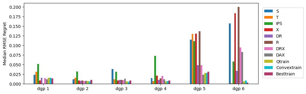
Figure 2: Median RMSE Regret for Each DGP.

Table 5: RMSE Regret For Fully-synthetic Datasets.

	DGP 1	DGP 2	DGP 3	DGP 4	DGP 5	DGP 6
S	[0.026 $\pm$ 0.012] 0.023 (0.047)	[0.014 $\pm$ 0.009] 0.012 (0.032)	[0.037 $\pm$ 0.010] 0.039 (0.051)	[0.017 $\pm$ 0.006] 0.015 (0.027)	[0.122 $\pm$ 0.034] 0.115 (0.186)	[0.159 $\pm$ 0.026] 0.157 (0.194)
T	[0.032 $\pm$ 0.007] 0.032 (0.042)	[0.016 $\pm$ 0.007] 0.016 (0.029)	[0.014 $\pm$ 0.011] 0.012 (0.036)	[0.008 $\pm$ 0.006] 0.007 (0.020)	[0.130 $\pm$ 0.027] 0.130 (0.168)	[0.005 $\pm$ 0.006] 0.002 (0.018)
IPS	[0.061 $\pm$ 0.047] 0.052 (0.143)	[0.045 $\pm$ 0.038] 0.032 (0.118)	[0.032 $\pm$ 0.008] 0.032 (0.047)	[0.075 $\pm$ 0.020] 0.073 (0.112)	[0.104 $\pm$ 0.044] 0.111 (0.164)	[0.058 $\pm$ 0.021] 0.058 (0.094)
X	[0.010 $\pm$ 0.009] 0.009 (0.025)	[0.010 $\pm$ 0.006] 0.009 (0.021)	[0.011 $\pm$ 0.009] 0.009 (0.023)	[0.021 $\pm$ 0.008] 0.021 (0.033)	[0.130 $\pm$ 0.026] 0.130 (0.168)	[0.175 $\pm$ 0.024] 0.183 (0.204)
DR	[0.017 $\pm$ 0.011] 0.016 (0.037)	[0.010 $\pm$ 0.007] 0.008 (0.022)	[0.013 $\pm$ 0.011] 0.011 (0.035)	[0.010 $\pm$ 0.007] 0.010 (0.022)	[0.052 $\pm$ 0.034] 0.048 (0.111)	[0.036 $\pm$ 0.015] 0.034 (0.063)
R	[0.004 $\pm$ 0.005] 0.001 (0.016)	[0.010 $\pm$ 0.005] 0.009 (0.019)	[0.015 $\pm$ 0.012] 0.010 (0.037)	[0.015 $\pm$ 0.008] 0.015 (0.029)	[0.135 $\pm$ 0.026] 0.136 (0.174)	[0.189 $\pm$ 0.024] 0.200 (0.215)
DRX	[0.017 $\pm$ 0.012] 0.015 (0.039)	[0.010 $\pm$ 0.008] 0.007 (0.026)	[0.012 $\pm$ 0.009] 0.010 (0.036)	[0.020 $\pm$ 0.008] 0.020 (0.032)	[0.053 $\pm$ 0.034] 0.048 (0.111)	[0.104 $\pm$ 0.035] 0.095 (0.176)
DAX	[0.018 $\pm$ 0.014] 0.012 (0.045)	[0.010 $\pm$ 0.008] 0.008 (0.025)	[0.018 $\pm$ 0.016] 0.013 (0.047)	[0.016 $\pm$ 0.016] 0.012 (0.042)	[0.031 $\pm$ 0.027] 0.024 (0.076)	[0.090 $\pm$ 0.028] 0.083 (0.140)
Besttrain	[0.017 $\pm$ 0.013] 0.014 (0.040)	[0.011 $\pm$ 0.008] 0.010 (0.027)	[0.012 $\pm$ 0.011] 0.009 (0.036)	[0.010 $\pm$ 0.009] 0.008 (0.021)	[0.036 $\pm$ 0.031] 0.032 (0.089)	[0.008 $\pm$ 0.013] 0.003 (0.041)
Convextrain	[0.017 $\pm$ 0.011] 0.016 (0.039)	[0.009 $\pm$ 0.008] 0.007 (0.027)	[0.008 $\pm$ 0.009] 0.006 (0.025)	[0.008 $\pm$ 0.007] 0.007 (0.020)	[0.033 $\pm$ 0.025] 0.028 (0.083)	[0.011 $\pm$ 0.009] 0.009 (0.027)
Qtrain	[0.016 $\pm$ 0.011] 0.015 (0.038)	[0.009 $\pm$ 0.007] 0.007 (0.023)	[0.009 $\pm$ 0.009] 0.006 (0.025)	[0.008 $\pm$ 0.007] 0.007 (0.021)	[0.033 $\pm$ 0.025] 0.028 (0.083)	[0.010 $\pm$ 0.010] 0.006 (0.026)
$\%$ Decrease w.r.t Best	1.264 $\%$ -7.700 $\%$	22.081 $\%$ 40.148 $\%$	41.138 $\%$ 44.073 $\%$	20.952 $\%$ 25.093 $\%$	11.236 $\%$ 11.446 $\%$	-13.003 $\%$ -49.579 $\%$
$\%$ Decrease w.r.t Convex	2.324 $\%$ 2.740 $\%$	0.119 $\%$ -6.044 $\%$	-4.316 $\%$ -8.569 $\%$	0.526 $\%$ 5.734 $\%$	0.080 $\%$ -0.636 $\%$	12.474 $\%$ 35.252 $\%$

Table 6: RMSE Regret For Semi-synthetic Datasets with Simple CATE.

	401k	welfare	poverty	star	criteo
S	[2042 $\pm$ 411.7] 2042 (2677)	[0.0947 $\pm$ 0.0248] 0.0929 (0.1346)	[0.0050 $\pm$ 0.0050] 0.0034 (0.0139)	[0.0055 $\pm$ 0.0059] 0.0035 (0.0174)	[0.00151 $\pm$ 0.00044] 0.0015 (0.00223)
T	[1172 $\pm$ 229.5] 1172 (1572)	[0.0546 $\pm$ 0.0267] 0.0573 (0.1035)	[0.0193 $\pm$ 0.0072] 0.0188 (0.0320)	[0.0224 $\pm$ 0.0211] 0.0169 (0.0670)	[0.00136 $\pm$ 0.00054] 0.0013 (0.00231)
IPS	[5845 $\pm$ 1489] 5513 (8983)	[0.7937 $\pm$ 0.0893] 0.7757 (0.9694)	[0.1739 $\pm$ 0.0373] 0.1731 (0.2329)	[0.6294 $\pm$ 0.2361] 0.5938 (1.0945)	[0.05433 $\pm$ 0.02190] 0.0459 (0.09577)
X	[302.6 $\pm$ 155.6] 289.2 (582.4)	[0.0337 $\pm$ 0.0170] 0.0319 (0.0649)	[0.0159 $\pm$ 0.0064] 0.0152 (0.0267)	[0.0145 $\pm$ 0.0158] 0.0096 (0.0490)	[0.00079 $\pm$ 0.00032] 0.0008 (0.00135)
DR	[581 $\pm$ 225.8] 587.6 (994.3)	[0.0522 $\pm$ 0.0195] 0.0494 (0.0876)	[0.0241 $\pm$ 0.0068] 0.0229 (0.0375)	[0.0206 $\pm$ 0.0165] 0.0194 (0.0431)	[0.00105 $\pm$ 0.00055] 0.0010 (0.00193)
R	[727.5 $\pm$ 217.9] 704.6 (1096)	[0.0872 $\pm$ 0.0174] 0.0889 (0.1157)	[0.0248 $\pm$ 0.0072] 0.0239 (0.0378)	[0.0280 $\pm$ 0.0176] 0.0254 (0.0540)	[0.00302 $\pm$ 0.00057] 0.0031 (0.00390)
DRX	[460.5 $\pm$ 194] 460.3 (801.7)	[0.0510 $\pm$ 0.0188] 0.0489 (0.0832)	[0.0240 $\pm$ 0.0069] 0.0223 (0.0390)	[0.0198 $\pm$ 0.0157] 0.0176 (0.0411)	[0.00082 $\pm$ 0.00040] 0.0008 (0.00161)
DAX	[446.6 $\pm$ 179.7] 444.6 (741.2)	[0.0727 $\pm$ 0.0173] 0.0718 (0.1047)	[0.0147 $\pm$ 0.0068] 0.0138 (0.0260)	[0.0133 $\pm$ 0.0170] 0.0083 (0.0389)	[0.00145 $\pm$ 0.00030] 0.0015 (0.00190)
Besttrain	[355 $\pm$ 147.9] 362.4 (585.7)	[0.0390 $\pm$ 0.0181] 0.0406 (0.0722)	[0.0075 $\pm$ 0.0068] 0.0060 (0.0194)	[0.0107 $\pm$ 0.0096] 0.0070 (0.0287)	[0.00081 $\pm$ 0.00040] 0.0008 (0.00161)
Convextrain	[362.3 $\pm$ 157.1] 371.5 (634.4)	[0.0289 $\pm$ 0.0156] 0.0275 (0.0557)	[0.0066 $\pm$ 0.0049] 0.0057 (0.0166)	[0.0095 $\pm$ 0.0093] 0.0062 (0.0284)	[0.00066 $\pm$ 0.00032] 0.0006 (0.00122)
Qtrain	[341.1 $\pm$ 157.1] 331.3 (634.2)	[0.0281 $\pm$ 0.0156] 0.0272 (0.0537)	[0.0061 $\pm$ 0.0049] 0.0051 (0.0165)	[0.0095 $\pm$ 0.0093] 0.0061 (0.0284)	[0.00060 $\pm$ 0.00032] 0.0006 (0.00112)
$\%$ Decrease w.r.t Best	4.0692 $\%$ 9.4008 $\%$	38.7569 $\%$ 49.2038 $\%$	22.8005 $\%$ 17.7918 $\%$	13.0432 $\%$ 15.7684 $\%$	34.8879 $\%$ 30.0913 $\%$
$\%$ Decrease w.r.t Convex	6.2148 $\%$ 12.1341 $\%$	2.6238 $\%$ 1.0101 $\%$	8.1161 $\%$ 13.0241 $\%$	0.2770 $\%$ 2.3870 $\%$	9.9629 $\%$ 8.5184 $\%$

Table 7: RMSE Regret For Semi-synthetic Datasets with Fitted CATE.

	401k	welfare	poverty	star	criteo
S	[115.1 $\pm$ 104.1] 98.59 (306.3)	[0.0029 $\pm$ 0.0018] 0.0029 (0.0061)	[0.0002 $\pm$ 0.0004] 0.0000 (0.0013)	[0.0843 $\pm$ 0.1903] 0.0000 (0.4518)	[0.00000 $\pm$ 0.00001] 0.0000 (0.00001)
T	[1526 $\pm$ 340.2] 1511 (2052)	[0.0033 $\pm$ 0.0014] 0.0031 (0.0056)	[0.0088 $\pm$ 0.0013] 0.0088 (0.0110)	[4.3250 $\pm$ 0.6061] 4.3450 (5.1982)	[0.00334 $\pm$ 0.00089] 0.0035 (0.00478)
IPS	[1643 $\pm$ 1291] 1212 (4731)	[0.0343 $\pm$ 0.0059] 0.0343 (0.0437)	[0.0219 $\pm$ 0.0151] 0.0181 (0.0575)	[345.6718 $\pm$ 130.7644] 321.2090 (563.5089)	[0.00227 $\pm$ 0.00107] 0.0024 (0.00376)
X	[431.7 $\pm$ 271.9] 400.8 (919.6)	[0.0039 $\pm$ 0.0017] 0.0037 (0.0069)	[0.0032 $\pm$ 0.0010] 0.0031 (0.0048)	[1.3916 $\pm$ 0.4319] 1.3608 (2.1141)	[0.00013 $\pm$ 0.00011] 0.0001 (0.00035)
DR	[321.8 $\pm$ 284.4] 259.5 (882.3)	[0.0063 $\pm$ 0.0021] 0.0060 (0.0103)	[0.0025 $\pm$ 0.0014] 0.0022 (0.0048)	[1.6791 $\pm$ 0.8769] 1.7604 (3.0720)	[0.00006 $\pm$ 0.00004] 0.0000 (0.00015)
R	[410.2 $\pm$ 216.7] 374 (837.5)	[0.0095 $\pm$ 0.0020] 0.0094 (0.0129)	[0.0068 $\pm$ 0.0011] 0.0068 (0.0086)	[0.8925 $\pm$ 0.4380] 0.7595 (1.7322)	[0.00081 $\pm$ 0.00008] 0.0008 (0.00094)
DRX	[314.5 $\pm$ 279.5] 251.4 (842.7)	[0.0063 $\pm$ 0.0021] 0.0059 (0.0103)	[0.0025 $\pm$ 0.0014] 0.0022 (0.0048)	[0.8536 $\pm$ 0.6130] 0.7277 (2.0083)	[0.00006 $\pm$ 0.00004] 0.0001 (0.00013)
DAX	[501.6 $\pm$ 254.7] 437.1 (1063)	[0.0052 $\pm$ 0.0015] 0.0050 (0.0080)	[0.0062 $\pm$ 0.0011] 0.0061 (0.0082)	[1.2216 $\pm$ 0.4937] 1.2192 (2.0556)	[0.00090 $\pm$ 0.00021] 0.0009 (0.00123)
Besttrain	[257.5 $\pm$ 262.1] 159.9 (812.1)	[0.0029 $\pm$ 0.0015] 0.0029 (0.0053)	[0.0017 $\pm$ 0.0020] 0.0009 (0.0057)	[2.0018 $\pm$ 1.4700] 1.6779 (4.7187)	[0.00002 $\pm$ 0.00003] 0.0000 (0.00010)
Convextrain	[266.2 $\pm$ 180.9] 245.3 (577.4)	[0.0019 $\pm$ 0.0012] 0.0019 (0.0040)	[0.0023 $\pm$ 0.0014] 0.0022 (0.0048)	[2.1629 $\pm$ 0.8906] 2.2012 (3.5904)	[0.00027 $\pm$ 0.00007] 0.0003 (0.00038)
Qtrain	[245.6 $\pm$ 183] 215.8 (579.5)	[0.0019 $\pm$ 0.0012] 0.0020 (0.0041)	[0.0021 $\pm$ 0.0014] 0.0020 (0.0047)	[2.0705 $\pm$ 0.9286] 2.0370 (3.5692)	[0.00024 $\pm$ 0.00006] 0.0002 (0.00035)
$\%$ Decrease w.r.t Best	4.8579 $\%$ -25.8868 $\%$	50.4544 $\%$ 46.1057 $\%$	-17.3363 $\%$ -55.4313 $\%$	-3.3152 $\%$ -17.6290 $\%$	-91.0409 $\%$ -100.0000 $\%$
$\%$ Decrease w.r.t Convex	8.4122 $\%$ 13.6626 $\%$	-0.7623 $\%$ -4.4831 $\%$	8.7545 $\%$ 9.9212 $\%$	4.4656 $\%$ 8.0570 $\%$	10.7980 $\%$ 11.0042 $\%$

Appendix E Proof of Main Theorem

In this section, we will be proving Theorem 3 in the main paper, which we also reproduce here:

Theorem 14 (Main Theorem).

Assume that for some function $\textsc{Error}(\hat{g})$:

$$P(\tilde{\ell}_{\theta,g_{0}}(Z)-\tilde{\ell}_{\theta^{\prime},g_{0}}(Z))-P(\tilde{\ell}_{\theta,\hat{g}}(Z)-\tilde{\ell}_{\theta^{\prime},\hat{g}}(Z))\leq\textsc{Error}(\hat{g})\,\|f_{\theta}-f_{\theta^{\prime}}\|^{\gamma}$$ (169)

for some $\gamma\in[0,1]$ and $\ell(f,g_{0})$ is $\sigma$-strongly convex in expectation with respect to $f$. Moreover, assume that the loss $\ell(Z;f(X),\hat{g})$ is $C_{b}(\hat{g})$-Lipszhitz with respect to $f(X)$, and both the loss and the candidate functions are uniformly bounded in $[-b,b]$ almost surely. For any $\mu\leq\min\{\nu,1-\nu\}\frac{\sigma}{14}$ and $\beta\geq\{\frac{8C_{b}^{2}(1-\nu)^{2}}{\mu},8\sqrt{3}bC_{b}(1-\nu),\frac{2C_{b}\nu(\nu C_{b}+\mu b)}{\mu}\}$, w.p. $1-\delta$:

$$R(\hat{\theta},g_{0})\leq~{} \min_{j=1}^{M}\left(R(e_{j},g_{0})+\frac{\beta}{n}\log(1/\pi_{j})\right)+O\left(\frac{\log(1/\delta)\max\{\frac{1}{\mu}C_{b}(\hat{g})^{2},b\,C_{b}(\hat{g})\}}{n}\right)+\left(\frac{1}{\mu}\right)^{\frac{\gamma}{2-\gamma}}\textsc{Error}(\hat{g})^{\frac{2}{2-\gamma}}$$ (170)

We remind some key definitions and assumptions from the main text. We assume that the function $\ell$ is $\sigma$-strongly convex in $f$ in expectation, i.e.:

$$P\left(\ell(Z;f^{\prime}(X),g_{0})-\ell(Z;f(X),g_{0})\right)\geq P\left(\langle\nabla_{f}\ell(Z;f(X),g_{0}),f^{\prime}(X)-f(X)\rangle\right)+\frac{\sigma}{2}\|f-f^{\prime}\|^{2}$$ (171)

We consider the modified loss, which penalizes the weight put on each model, based on the individual model performance:

$$\tilde{\ell}_{\theta,g}(Z)=~{} (1-\nu)\ell_{\theta,g}(Z)+\nu\sum_{j}\theta_{j}\ell_{e_{j},g}(Z) \tilde{R}(\theta,g)=~{} P\tilde{\ell}_{\theta,g}(Z)$$ (172)

We also define with:

$$K(\theta):=~{} \sum_{j}\theta_{j}\log(1/\pi_{j})$$ (173)

Then the Q-aggregation ensemble is defined as:

$$\hat{\theta}=~{} \arg\min_{\theta}P_{n}\tilde{\ell}_{\theta,\hat{g}}(Z)+\frac{\beta}{n}K(\theta)$$ (174)

We introduce some population quantities that will play a key role in our analysis. Define:

$$V(\theta):=~{} \sum_{j}\theta_{j}\|f_{j}-f_{\theta}\|^{2}$$ (175)

$$H(\theta,g):=\tilde{R}(\theta,g)+\mu V(\theta)+\frac{\beta}{n}K(\theta)$$

and define:

$$\theta^{*}=~{} \arg\min_{\theta}\tilde{R}(\theta,g_{0})+\mu V(\theta)+\frac{\beta}{n}K(\theta)~{}=~{}\arg\min_{\theta}H(\theta,g_{0})$$ (176)

Then we introduce the shorthand notation and invoke the error decomposition assumption:

$${\cal E}(\hat{g}):=~{} P(\tilde{\ell}_{\hat{\theta},g_{0}}(Z)-\tilde{\ell}_{\theta^{*},g_{0}}(Z))-P(\tilde{\ell}_{\hat{\theta},\hat{g}}(Z)-\tilde{\ell}_{\theta^{*},\hat{g}}(Z))~{}\leq~{}\textsc{Error}(\hat{g})\,\|f_{\hat{\theta}}-f_{\theta^{*}}\|^{\gamma}$$ (178)

Lemma 15.

If $\ell(Z;f(X),g)$ is $\sigma(g)$-strongly convex in expectation with respect to $f$, then for any $\theta,\theta^{\prime}\in\Theta$:

$$R(\theta,g)-R(\theta^{\prime},g)\geq\langle\nabla R(\theta^{\prime},g),\theta-\theta^{\prime}\rangle+\frac{\sigma(g)}{2}\|f_{\theta}-f_{\theta^{\prime}}\|^{2}$$ (179)

Proof.

Let $F$ be the random column vector defined as $F:=[f_{1}(X)\cdots f_{M}(X)]$. Note that by the chain rule:

$$\langle\nabla_{\theta}\ell(Z;f_{\theta}^{\prime}(X),g),\theta-\theta^{\prime}\rangle =\langle(\nabla_{\theta}(f_{\theta^{\prime}}(X)))^{\top}\nabla_{f}\ell(Z;f_{\theta^{\prime}}(X),g),\theta-\theta^{\prime}\rangle$$ (180)

$$=\langle F\nabla_{f}\ell(Z;f_{\theta^{\prime}}(X),g),\theta-\theta^{\prime}\rangle$$ (181)

$$=\nabla_{f}\ell(Z;f_{\theta^{\prime}}(X),g))^{\top}F^{\top}(\theta-\theta^{\prime})$$ (182)

$$=\langle\nabla_{f}\ell(Z;f_{\theta^{\prime}}(X),g),F^{\top}(\theta-\theta^{\prime})\rangle$$ (183)

$$=\langle\nabla_{f}\ell(Z;f_{\theta^{\prime}}(X),g),f_{\theta}(X)-f_{\theta}^{\prime}(X)\rangle$$ (184)

Taking expectation over $Z$, we have:

$$\langle\nabla_{\theta}R(\theta^{\prime}),\theta-\theta^{\prime}\rangle=~{} \langle\nabla_{\theta}\mathbb{E}\left[\ell(Z;f_{\theta}^{\prime}(X),g)\right],\theta-\theta^{\prime}\rangle$$ (185)

$$=~{} \mathbb{E}\left[\langle\nabla_{\theta}\ell(Z;f_{\theta}^{\prime}(X),g),\theta-\theta^{\prime}\rangle\right]$$ (186)

$$=~{} \mathbb{E}\left[\langle\nabla_{f}\ell(Z;f_{\theta^{\prime}}(X),g),f_{\theta}(X)-f_{\theta}^{\prime}(X)\rangle\right]$$ (187)

The result then follows by the definition of $\sigma(g)$-strong convexity in expectation of the function $\ell(f,g)$ and the definition of $R(\theta,g)$. ∎

Lemma 16.

If $R(\theta,g)$ is $\sigma(g)$-strongly convex in expectation, then for any $\theta\in\Theta$:

$$\tilde{R}(\theta,g)\geq R(\theta,g)+\frac{\nu\sigma(g)}{2}V(\theta)$$ (188)

Proof.

By $\sigma$-strong convexity of the loss and Lemma 15, we have that:

$$R(e_{j},g)-R(\theta,g)\geq\langle\nabla R(\theta,g),e_{j}-\theta\rangle+\frac{\sigma(g)}{2}\|f_{j}-f_{\theta}\|^{2}$$ (189)

Multiplying each equation by $\theta_{j}$ and summing across $j$, yields:

$$R(\theta,g)\leq\sum_{j}\theta_{j}R(e_{j},g)-\frac{\sigma(g)}{2}V(\theta)$$ (190)

where we used the fact that $\sum_{j}\theta_{j}=1$ and $\sum_{j}\theta_{j}\langle\nabla R(\theta,g),e_{j}-\theta\rangle=0$.

Thus we have that:

$$\tilde{R}(\theta,g)=~{} (1-\nu)R(\theta,g)+\nu\sum_{j}\theta_{j}R(e_{j},g)$$ (191)

$$\geq~{} (1-\nu)R(\theta,g)+\nu R(\theta,g)+\frac{\nu\sigma(g)}{2}V(\theta)$$ (192)

$$=~{} R(\theta,g)+\frac{\nu\sigma(g)}{2}V(\theta)$$ (193)

∎

Lemma 17.

If $\ell(Z;f(X),g_{0})$ is $\sigma$-strongly convex in $f$, in expectation, and $\theta_{*}=\operatorname*{arg\,min}_{\theta\in\Theta}H(\theta,g_{0})$, then for any $\theta\in\Theta$:

$$H(\theta,g_{0})-H(\theta^{*},g_{0})\geq\left(\frac{(1-\nu)\sigma}{2}-\mu\right)\|f_{\theta}-f_{\theta^{*}}\|^{2}$$ (194)

Proof.

By Lemma 15 we have:

$$R(\theta,g_{0})-R(\theta^{\prime},g_{0})\geq\langle\nabla R(\theta^{\prime},g_{0}),\theta-\theta^{\prime}\rangle+\frac{\sigma}{2}\|f_{\theta}-f_{\theta^{\prime}}\|^{2}$$ (195)

Now let $q(Z;\theta,g)=\sum_{j=1}^{M}\theta_{j}\ell(Z;f_{e_{j}}(X),g)$ and $L_{e}(g)=[\ell(Z;f_{e_{1}}(X),g)\cdots\ell(Z;f_{e_{M}}(X),g)]^{T}$ and let $Q(\theta,g)=\mathbb{E}\left[q(Z;\theta,g)\right]$. We have that:

$$q(Z;\theta,g)-q(Z;\theta^{\prime},g) =\sum_{j=1}^{M}\ell(Z;f_{e_{j}}(X),g)(\theta_{j}-\theta^{\prime}_{j})=\langle{L_{e}(g),\theta-\theta^{\prime}}\rangle=\langle\nabla q(Z;\theta^{\prime},g),\theta-\theta^{\prime}\rangle$$ (196)

By taking the expectation over $Z$:

$$Q(\theta,g)-Q(\theta^{\prime},g)=\sum_{j=1}^{M}\theta_{j}R(e_{j},g)-\sum_{j=1}^{M}\theta_{j}^{\prime}R(e_{j},g)=\langle\nabla Q(\theta^{\prime},g),\theta-\theta^{\prime}\rangle$$ (197)

By adding Equations (195) and (197) we have that:

$$\tilde{R}(\theta,g_{0})-\tilde{R}(\theta^{\prime},g_{0})=~{} (1-\nu)(R(\theta,g_{0})-R(\theta^{\prime},g_{0}))+\nu(Q(\theta,g_{0})-Q(\theta^{\prime},g_{0}))$$ (198)

$$\geq~{} (1-\nu)\langle\nabla R(\theta^{\prime},g_{0}),\theta-\theta^{\prime}\rangle+\nu\langle\nabla Q(\theta^{\prime},g_{0}),\theta-\theta^{\prime}\rangle+\frac{(1-\nu)\sigma}{2}\|f_{\theta}-f_{\theta^{\prime}}\|^{2}$$ (199)

$$\geq~{} \langle\nabla\tilde{R}(\theta^{\prime},g_{0}),\theta-\theta^{\prime}\rangle+\frac{(1-\nu)\sigma}{2}\|f_{\theta}-f_{\theta^{\prime}}\|^{2}$$ (200)

meaning that $\tilde{R}$ will also be $(1-\nu)\sigma$-strongly convex in $\theta$. We also have that for any $\theta,\theta^{\prime}$:

$$V(\theta)-V(\theta^{\prime})=\langle\nabla V(\theta^{\prime}),\theta-\theta^{\prime}\rangle-\|f_{\theta}-f_{\theta^{\prime}}\|_{2}^{2}$$ (201)

which implies that $V(\theta)$ is at most 2-strongly concave. We also have:

$$K(\theta)-K(\theta^{\prime})=\sum_{j}(\theta_{j}-\theta^{\prime}_{j})\log(1/\pi_{j})=\langle\nabla K(\theta^{\prime}),\theta-\theta^{\prime}\rangle$$ (202)

Adding the three inequalities and substituting $\theta^{\prime}$ with $\theta^{*}$ we have:

$$H(\theta,g_{0})-H(\theta^{*},g_{0})\geq\langle\nabla H(\theta^{*},g_{0}),\theta-\theta^{*}\rangle+\left(\frac{(1-\nu)\sigma}{2}-\mu\right)\|f_{\theta}-f_{\theta^{*}}\|^{2}$$ (203)

Note that by the optimality of $\theta^{*}$ over the convex set $\Theta$ we have that $\langle\nabla H(\theta^{*},g_{0}),\theta-\theta^{*}\rangle\geq 0$, which immediately yields the statement we want to prove. ∎

Lemma 18.

Define the centered and offset empirical processes:

$$Z_{n,1}=~{} (1-\nu)(P-P_{n})(\ell_{\hat{\theta},\hat{g}}(Z)-\ell_{\theta^{*},\hat{g}}(Z))-\mu\sum_{j}\hat{\theta}_{j}\|f_{j}-f_{\theta^{*}}\|^{2}{-\frac{1}{s}K(\hat{\theta})}$$ (204)

$$Z_{n,2}=~{} \nu(P-P_{n})\sum_{j}(\hat{\theta}_{j}-\theta_{j}^{*})\ell_{e_{j},\hat{g}}(Z)-\mu\hat{\theta}^{\top}H\theta^{*}{-\frac{1}{s}K(\hat{\theta})} H_{ij}=\|f_{i}-f_{j}\|^{2}$$ (205)

where $s$ is a positive number. Assume that:

$${\cal E}(\hat{g}):=P(\tilde{\ell}_{\hat{\theta},g_{0}}(Z)-\tilde{\ell}_{\theta^{*},g_{0}}(Z))-P(\tilde{\ell}_{\hat{\theta},\hat{g}}(Z)-\tilde{\ell}_{\theta^{*},\hat{g}}(Z))\leq\textsc{Error}(\hat{g})\,\|f_{\theta}-f_{\theta^{*}}\|$$ (206)

and $\ell(Z;f(X),g_{0})$ is $\sigma$-strongly convex in expectation with respect to $f$. For $\beta\geq\frac{4n}{s}$ and $\mu\leq\min\{\nu,1-\nu\}\frac{\sigma}{14}$:

$$R(\hat{\theta})\leq\min_{j}[R(e_{j},g_{0}){+\frac{\beta}{n}\log(1/\pi_{j})}]+2\,(Z_{n,1}+Z_{n,2})+\frac{1}{\mu}\textsc{Error}(\hat{g})^{2}$$ (207)

Proof.

$$\tilde{R}(\hat{\theta},g_{0})-\tilde{R}(\theta^{*},g_{0})=~{} P(\tilde{\ell}_{\hat{\theta},g_{0}}(Z)-\tilde{\ell}_{\theta^{*},g_{0}}(Z))$$ (208)

$$=~{} P(\tilde{\ell}_{\hat{\theta},\hat{g}}(Z)-\tilde{\ell}_{\theta^{*},\hat{g}}(Z))+{\cal E}(\hat{g})$$ (209)

$$\leq~{} (P-P_{n})(\tilde{\ell}_{\hat{\theta},\hat{g}}(Z)-\tilde{\ell}_{\theta^{*},\hat{g}}(Z))+{\cal E}(\hat{g}){-\frac{\beta}{n}(K(\hat{\theta})-K(\theta^{*}))} \hat{\theta} P_{n}(\tilde{\ell}_{\hat{\theta},\hat{g}}(Z)-\tilde{\ell}_{\theta^{*},\hat{g}}(Z)){+\frac{\beta}{n}(K(\hat{\theta})-K(\theta^{*}))}\leq 0$$ (By optimality of , )

$$=~{} \mu\sum_{j}\hat{\theta}_{j}\|f_{j}-f_{\theta^{*}}\|^{2}+\mu\hat{\theta}^{\top}H\theta^{*}+Z_{n,1}+Z_{n,2}+{\cal E}(\hat{g})$$ (210)

$${-\frac{\beta}{n}(K(\hat{\theta})-K(\theta^{*}))+\frac{2}{s}K(\hat{\theta})} Z_{n,1},Z_{n,2}$$ (definition of )

By simple algebraic manipulations note that for any $\theta\in\Theta$:

$$\sum_{j}\hat{\theta}_{j}\|f_{j}-f_{\theta^{*}}\|^{2}=V(\hat{\theta})+\|f_{\hat{\theta}}-f_{\theta^{*}}\|^{2}$$ (211)

$$\hat{\theta}^{\top}H\theta^{*}=V(\hat{\theta})+V(\theta^{*})+\|f_{\hat{\theta}}-f_{\theta^{*}}\|^{2}$$ (212)

Letting $Z_{n}=Z_{n,1}+Z_{n,2}$, we have:

$$\tilde{R}(\hat{\theta},g_{0})-\tilde{R}(\theta^{*},g_{0})\leq~{} 2\mu V(\hat{\theta})+\mu V(\theta^{*})+2\mu\|f_{\hat{\theta}}-f_{\theta^{*}}\|^{2}+Z_{n}+{\cal E}(\hat{g}){-\frac{\beta}{n}(K(\hat{\theta})-K(\theta^{*}))+\frac{2}{s}K(\hat{\theta})}$$ (213)

$$\leq~{} 2\mu V(\hat{\theta})+\mu V(\theta^{*})+2\mu\|f_{\hat{\theta}}-f_{\theta^{*}}\|^{2}+Z_{n}+\textsc{Error}(\hat{g})\,\|f_{\hat{\theta}}-f_{\theta^{*}}\|^{\gamma}$$ (214)

$${-\frac{\beta}{n}(K(\hat{\theta})-K(\theta^{*}))+\frac{2}{s}K(\hat{\theta})}$$ (215)

By Young’s inequality, for any $a\geq 0$ and $b\geq 0$, we have $a\,b\leq\frac{a^{p}}{p}+\frac{b^{q}}{q}$, such that $\frac{1}{p}+\frac{1}{q}=1$. Taking $a=\left(\frac{\gamma}{2\mu}\right)^{\gamma/2}\textsc{Error}(\hat{g})$ and $b=\left(\frac{2\mu}{\gamma}\right)^{\gamma/2}\|f_{\hat{\theta}}-f_{\theta^{*}}\|^{\gamma}$ and $q=2/\gamma$ and $p=\frac{1}{1-1/q}=\frac{1}{1-\gamma/2}=\frac{2}{2-\gamma}$

$$\textsc{Error}(\hat{g})\,\|f_{\hat{\theta}}-f_{\theta^{*}}\|^{\gamma}\leq\underbrace{\frac{2}{2-\gamma}\left(\frac{\gamma}{2\mu}\right)^{\frac{\gamma}{2-\gamma}}\textsc{Error}(\hat{g})^{\frac{2}{2-\gamma}}}_{{\cal A}(\hat{g})}+\mu\|f_{\hat{\theta}}-f_{\theta^{*}}\|^{2}$$ (216)

Thus we can derive:

$$\tilde{R}(\hat{\theta},g_{0})-\tilde{R}(\theta^{*},g_{0})\leq~{} 2\mu V(\hat{\theta})+\mu V(\theta^{*})+3\mu\|f_{\hat{\theta}}-f_{\theta^{*}}\|^{2}+Z_{n}+{\cal A}(\hat{g})$$ (217)

$${-\frac{\beta}{n}(K(\hat{\theta})-K(\theta^{*}))+\frac{2}{s}K(\hat{\theta})}$$ (218)

By Lemma 17, we have:

$$\tilde{R}(\hat{\theta},g_{0})-\tilde{R}(\theta^{*},g_{0})\geq~{} \mu(V(\theta^{*})-V(\hat{\theta})){+\frac{\beta}{n}(K(\theta^{*})-K(\hat{\theta}))}+\left(\frac{(1-\nu)\sigma}{2}-\mu\right)\|f_{\hat{\theta}}-f_{\theta^{*}}\|^{2}$$ (219)

$$\geq~{} \mu(V(\theta^{*})-V(\hat{\theta})){+\frac{\beta}{n}(K(\theta^{*})-K(\hat{\theta}))}+6\mu\|f_{\hat{\theta}}-f_{\theta^{*}}\|^{2} \mu\leq\frac{(1-\nu)\sigma}{14}\implies\frac{(1-\nu)\sigma}{2}\geq 7\mu$$ (Since: )

Combining the latter upper and lower bound on $\tilde{R}(\hat{\theta},g_{0})-\tilde{R}(\theta^{*},g_{0})$, we have:

$$3\mu\|f_{\hat{\theta}}-f_{\theta^{*}}\|^{2}\leq 3\mu V(\hat{\theta})+Z_{n}{+\frac{2}{s}K(\hat{\theta})}+{\cal A}(\hat{g})$$ (220)

Plugging the bound on $3\mu\|f_{\hat{\theta}}-f_{\theta^{*}}\|^{2}$ back into Equation (218) we have:

$$\tilde{R}(\hat{\theta},g_{0})-\tilde{R}(\theta^{*},g_{0})\leq~{} 5\mu V(\hat{\theta})+\mu V(\theta^{*})+2\,Z_{n}+2\,{\cal A}(\hat{g})$$ (221)

$${+\frac{\beta}{n}(K(\theta^{*})-K(\hat{\theta}))+\frac{4}{s}K(\hat{\theta})}$$ (222)

By Lemma 16, we have:

$$R(\hat{\theta},g_{0})\leq~{} \tilde{R}(\theta^{*},g_{0})+\mu V(\theta^{*})+\left(5\mu-\frac{\nu\sigma(g_{0})}{2}\right)V(\hat{\theta})+2Z_{n}+2{\cal A}(\hat{g})$$ (223)

$${+\frac{\beta}{n}K(\theta^{*})+\left(\frac{4}{s}-\frac{\beta}{n}\right)K(\hat{\theta})}$$ (224)

$$\leq~{} \tilde{R}(\theta^{*},g_{0})+\mu V(\theta^{*}){+\frac{\beta}{n}K(\theta^{*})}+2Z_{n}+2{\cal A}(\hat{g}) \mu\leq\frac{\nu\sigma}{10} V(\hat{\theta})>0 \beta\geq\frac{4n}{s} K(\hat{\theta}\geq 0)$$ (since , , and )

$$=~{} \min_{\theta\in\Theta}[\tilde{R}(\theta,g_{0})+\mu V(\theta){+\frac{\beta}{n}K(\theta^{*})}]+2Z_{n}+2{\cal A}(\hat{g}) \theta_{*} H(\theta,g_{0})$$ (Since minimizes )

$$\leq~{} \min_{j}[\tilde{R}(e_{j},g_{0})+\mu V(e_{j}){+\frac{\beta}{n}\log(1/\pi_{j})}]+2Z_{n}+2{\cal A}(\hat{g})$$ (225)

$$=~{} \min_{j}[R(e_{j},g_{0}){+\frac{\beta}{n}\log(1/\pi_{j})}]+2Z_{n}+2{\cal A}(\hat{g}) \tilde{R}(e_{j},g_{0})=R(e_{j},g_{0}) V(e_{j})=0 e_{j}$$ (Since and for all )

∎

E.1 Concentration of offset empirical processes

Lemma 19.

Assuming that the loss $\ell(f(X),\hat{g})$ is $C_{b}$ lipschitz in $f(X)$ and all $f_{i}(X)$ are bounded in $[-b,b]$, almost surely, then for any positive $s\leq\min\left\{\frac{\mu n}{(2C_{b}(1-\nu))^{2}},\frac{n}{2\sqrt{3}bC_{b}(1-\nu)}\right\}$:

$${\mathrm{Pr}\left(Z_{n,1}\geq\frac{\log(1/\delta)}{s}\right)\leq\delta}$$ (226)

Proof.

By Lemma 21 it suffices to show that:

$${I:=\mathbb{E}\left[\exp\left\{sZ_{n,1}\right\}\right]\leq 1}$$ (227)

By symmetrization (sym.) and contraction (contr.):

$$I=~{} \mathbb{E}\left[\exp\left\{s\left((1-\nu)(P-P_{n})(\ell_{\hat{\theta}}(Z)-\ell_{\theta^{*}}(Z))-\mu\sum_{j}\hat{\theta}_{j}\|f_{j}-f_{\theta^{*}}\|^{2}{-\frac{1}{s}\sum_{j}\hat{\theta}_{j}\log(1/\pi_{j})}\right)\right\}\right]$$ (228)

$$\leq~{} \mathbb{E}\left[\exp\left\{s\max_{\theta}\left((1-\nu)(P-P_{n})(\ell_{\theta}(Z)-\ell_{\theta^{*}}(Z))-\mu\sum_{j}\theta_{j}\|f_{j}-f_{\theta^{*}}\|^{2}{+\frac{1}{s}\sum_{j}\theta_{j}\log(\pi_{j})}\right)\right\}\right]$$ (229)

$$\leq~{} \mathbb{E}\left[\exp\left\{s\max_{\theta}\left(2\,(1-\nu)P_{n,\epsilon}(\ell_{\theta}(Z)-\ell_{\theta^{*}}(Z))-\mu\sum_{j}\theta_{j}\|f_{j}-f_{\theta^{*}}\|^{2}{+\frac{1}{s}\sum_{j}\theta_{j}\log(\pi_{j})}\right)\right\}\right]$$ (sym.)

$$\leq~{} \mathbb{E}\left[\exp\left\{s\max_{\theta}\left(2\,(1-\nu)C_{b}P_{n,\epsilon}(f_{\theta}(Z)-f_{\theta^{*}}(Z))-\mu\sum_{j}\theta_{j}\|f_{j}-f_{\theta^{*}}\|^{2}+\frac{1}{s}\sum_{j}\theta_{j}\log(\pi_{j})\right)\right\}\right]$$ (contr.)

Since the quantity:

$$2\,(1-\nu)C_{b}P_{n,\epsilon}(f_{\theta}(Z)-f_{\theta^{*}}(Z))-\mu\sum_{j}\theta_{j}\|f_{j}-f_{\theta^{*}}\|^{2}+\frac{1}{s}\sum_{j}\theta_{j}\log(\pi_{j})$$ (230)

is a linear function of $\theta$ (recall that $f_{\theta}=\sum_{j}\theta_{j}f_{j}$), the maximum over $\theta$ is attained at one of $e_{1},\ldots,e_{M}$. Thus:

$$I\leq~{} \mathbb{E}\left[\exp\left\{s\max_{j}\left(2\,(1-\nu)C_{b}P_{n,\epsilon}(f_{j}(Z)-f_{\theta^{*}}(Z))-\mu\|f_{j}-f_{\theta^{*}}\|^{2}{+\frac{1}{s}\log(\pi_{j})}\right)\right\}\right]$$ (231)

$$\leq~{} \mathbb{E}\left[\max_{j}{\pi_{j}}\exp\left\{s\left(2\,(1-\nu)C_{b}P_{n,\epsilon}(f_{j}(Z)-f_{\theta^{*}}(Z))-\mu\|f_{j}-f_{\theta^{*}}\|^{2}\right)\right\}\right]$$ (232)

$$\leq~{} \mathbb{E}\left[\sum_{j}{\pi_{j}}\exp\left\{s\left(2\,(1-\nu)C_{b}P_{n,\epsilon}(f_{j}(Z)-f_{\theta^{*}}(Z))-\mu\|f_{j}-f_{\theta^{*}}\|^{2}\right)\right\}\right]$$ (233)

$$=~{} \sum_{j}{\pi_{j}}\mathbb{E}\left[\exp\left\{s\left(2\,(1-\nu)C_{b}P_{n,\epsilon}(f_{j}(Z)-f_{\theta^{*}}(Z))-\mu\|f_{j}-f_{\theta^{*}}\|^{2}\right)\right\}\right]$$ (234)

$$=~{} \sum_{j}{\pi_{j}}\mathbb{E}_{Z_{1:n}}\mathbb{E}_{\epsilon}\left[\exp\left\{s\left(2\,(1-\nu)C_{b}P_{n,\epsilon}(f_{j}(Z)-f_{\theta^{*}}(Z))-\mu\|f_{j}-f_{\theta^{*}}\|^{2}\right)\right\}\right]$$ (235)

$$=~{} \sum_{j}{\pi_{j}}\mathbb{E}_{Z_{1:n}}\left[\mathbb{E}_{\epsilon}\left[\exp\left\{s2\,(1-\nu)C_{b}P_{n,\epsilon}(f_{j}(Z)-f_{\theta^{*}}(Z))\right\}\right]\exp\left\{-s\mu\|f_{j}-f_{\theta^{*}}\|^{2}\right\}\right]$$ (236)

By Hoeffding’s inequality in Lemma 22, we can bound the first term in the product:

$$\mathbb{E}_{\epsilon}\left[\exp\left\{s2\,(1-\nu)C_{b}P_{n,\epsilon}(f_{j}(Z)-f_{\theta^{*}}(Z))\right\}\right]\leq\exp\left\{\frac{2s^{2}}{n}\,(1-\nu)^{2}C_{b}^{2}P_{n}(f_{j}(Z)-f_{\theta^{*}}(Z))^{2}\right\}$$ (237)

Thus we have:

$$I\leq~{} \sum_{j}{\pi_{j}}\mathbb{E}_{Z_{1:n}}\left[\exp\left\{\frac{2s^{2}}{n}\,(1-\nu)^{2}C_{b}^{2}P_{n}(f_{j}(Z)-f_{\theta^{*}}(Z))^{2}\right\}\,\exp\left\{-s\mu\|f_{j}-f_{\theta^{*}}\|^{2}\right\}\right]$$ (238)

$$=~{} \sum_{j}{\pi_{j}}\mathbb{E}_{Z_{1:n}}\left[\exp\left\{\frac{2s^{2}}{n}\,(1-\nu)^{2}C_{b}^{2}P_{n}(f_{j}(Z)-f_{\theta^{*}}(Z))^{2}\right\}\,\exp\left\{-s\mu P(f_{j}(Z)-f_{\theta^{*}}(Z))^{2}\right\}\right]$$ (239)

$$=~{} \sum_{j}{\pi_{j}}\mathbb{E}_{Z_{1:n}}\left[\exp\left\{\frac{2s^{2}\,(1-\nu)^{2}C_{b}^{2}}{n}\left(P_{n}-\frac{\mu\,n}{2s(1-\nu)^{2}C_{b}^{2}}P\right)(f_{j}(Z)-f_{\theta^{*}}(Z))^{2}\right\}\right]$$ (240)

Since $s$ is small enough such that: $\frac{\mu\,n}{2s(1-\nu)^{2}C_{b}^{2}}\geq 2$ (which is satisfied by our assumptions on $s$), we have that:

$$I\leq~{} \sum_{j}\pi_{j}\mathbb{E}_{Z_{1:n}}\left[\exp\left\{\frac{2s^{2}\,(1-\nu)^{2}C_{b}^{2}}{n}\left(P_{n}-2P\right)(f_{j}(Z)-f_{\theta^{*}}(Z))^{2}\right\}\right]$$ (241)

$$=~{} \sum_{j}\pi_{j}\mathbb{E}_{Z_{1:n}}\left[\exp\left\{\frac{2s^{2}\,(1-\nu)^{2}C_{b}^{2}}{n}\left(\left(P_{n}-P\right)(f_{j}(Z)-f_{\theta^{*}}(Z))^{2}-P(f_{j}(Z)-f_{\theta^{*}}(Z))^{2}\right)\right\}\right]$$ (242)

Since $f_{j}(Z)\in[-b,b]$, we have that $f_{j}(Z)-f_{\theta^{*}}(Z)\in[-2b,2b]$. Thus:

$$(f_{j}(Z)-f_{\theta^{*}}(Z))^{2}\geq\frac{(f_{j}(Z)-f_{\theta^{*}}(Z))^{2}}{4b^{2}}(f_{j}(Z)-f_{\theta^{*}}(Z))^{2}=\frac{1}{4b^{2}}(f_{j}(Z)-f_{\theta^{*}}(Z))^{4}.$$ (243)

Thus:

$$I\leq~{} \sum_{j}\pi_{j}\mathbb{E}_{Z_{1:n}}\left[\exp\left\{\frac{2s^{2}\,(1-\nu)^{2}C_{b}^{2}}{n}\left(\left(P_{n}-P\right)(f_{j}(Z)-f_{\theta^{*}}(Z))^{2}-\frac{1}{4b^{2}}P(f_{j}(Z)-f_{\theta^{*}}(Z))^{4}\right)\right\}\right]$$ (244)

It suffices to show that each of the summands is upper bounded by $1$. Then their weighted average is also upper bounded by $1$.

Applying Lemma 23 with:

$$V_{i}=~{} (f_{j}(Z_{i})-f_{\theta^{*}}(Z_{i}))^{2}$$ (245)

$$c=~{} 4b^{2}$$ (246)

$$\lambda=~{} \frac{2s^{2}(1-\nu)^{2}C_{b}^{2}}{n^{2}}$$ (247)

$$c_{0}=~{} \frac{1}{4b^{2}}$$ (248)

we have that as long as:

$$\lambda:=\frac{2s^{2}(1-\nu)^{2}C_{b}^{2}}{n^{2}}\leq\frac{2c_{0}}{1+2c_{0}c}=:\frac{2\cdot 1/4b^{2}}{1+2}=\frac{1}{6b^{2}}$$ (249)

Then:

$$\mathbb{E}_{Z_{1:n}}\left[\exp\left\{\frac{2s^{2}\,(1-\nu)^{2}C_{b}^{2}}{n}\left(\left(P_{n}-P\right)(f_{j}(Z)-f_{\theta^{*}}(Z))^{2}-\frac{1}{4b^{2}}P(f_{j}(Z)-f_{\theta^{*}}(Z))^{4}\right)\right\}\right]\leq 1$$ (250)

Thus we need that:

$$s\leq\frac{n}{2\sqrt{3}b(1-\nu)C_{b}}$$ (251)

which is satisfied by our assumptions on $s$. ∎

Lemma 20.

Assuming that the loss $\ell(f(X),\hat{g})$ is $C_{b}$ lipschitz in $f(X)$ and bounded in $[-b,b]$, for any positive $s\leq\frac{2\mu n}{C_{b}\nu(\nu C_{b}+4\mu b)}$:

$$\mathrm{Pr}\left(Z_{n,2}\geq\frac{\log(1/\delta)}{s}\right)\leq\delta$$ (252)

Proof.

It suffices to show that:

$$I:=\mathbb{E}\left[\exp\left\{sZ_{n,2})\right\}\right]\leq 1$$ (253)

By definition of $Z_{n,2}$:

$$I=~{} \mathbb{E}\left[\exp\left\{s\left(\nu(P-P_{n})\sum_{j}(\hat{\theta}_{j}-\theta_{j}^{*})\ell_{e_{j}}(Z)-\mu\hat{\theta}^{\top}H\theta^{*}-\frac{1}{s}\sum_{j}\hat{\theta}_{j}\log(1/\pi_{j})\right)\right\}\right]$$ (254)

$$=~{} \mathbb{E}\left[\exp\left\{s\left(\nu(P-P_{n})\sum_{j}\hat{\theta}_{j}\ell_{e_{j}}(Z)+\frac{1}{s}\sum_{j}\hat{\theta}_{j}\log(\pi_{j})\right)\right\}\exp\left\{s\left(-\nu(P-P_{n})\sum_{j}\theta_{j}^{*}\ell_{e_{j}}(Z)-\mu\hat{\theta}^{\top}H\theta^{*}\right)\right\}\right]$$ (255)

Note that:

$$-\nu(P-P_{n})\sum_{j}\theta_{j}^{*}\ell_{e_{j}}(Z)-\mu\hat{\theta}^{\top}H\theta^{*}=~{} \sum_{j}\theta_{j}^{*}\left(-\nu(P-P_{n})\ell_{e_{j}}(Z)-\mu\hat{\theta}^{\top}H_{\cdot,j}\right)$$ (256)

$$=~{} \sum_{j}\theta_{j}^{*}\underbrace{\left(-\nu(P-P_{n})\ell_{e_{j}}(Z)-\mu\sum_{k}\hat{\theta}_{k}\|f_{k}-f_{j}\|^{2}\right)}_{\Phi_{j}}$$ (257)

Thus:

$$I=~{} \mathbb{E}\left[\exp\left\{s\left(\nu(P-P_{n})\sum_{j}\hat{\theta}_{j}\ell_{e_{j}}(Z)+\frac{1}{s}\sum_{j}\hat{\theta}_{j}\log(\pi_{j})\right)\right\}\exp\left\{\sum_{j}\theta_{j}^{*}s\Phi_{j}\right\}\right]$$ (258)

By Jensen’s inequality:

$$\exp\left\{\sum_{j}\theta_{j}^{*}s\Phi_{j}\right\}\leq\sum_{j}\theta_{j}^{*}\exp\left\{s\Phi_{j}\right\}$$ (259)

Thus:

$$I\leq~{} \sum_{j}\theta_{j}^{*}\mathbb{E}\left[\exp\left\{s\left(\nu(P-P_{n})\sum_{k}\hat{\theta}_{k}\ell_{e_{k}}(Z){+\frac{1}{s}\sum_{k}\hat{\theta}_{k}\log(\pi_{k})}\right)\right\}\exp\left\{s\Phi_{j}\right\}\right]$$ (260)

$$=~{} \sum_{j}\theta_{j}^{*}\mathbb{E}\left[\exp\left\{s\left(\nu(P-P_{n})\sum_{k}\hat{\theta}_{k}\ell_{e_{k}}(Z)+\Phi_{j}{+\frac{1}{s}\sum_{k}\hat{\theta}_{k}\log(\pi_{k})}\right)\right\}\right]$$ (261)

$$=~{} \sum_{j}\theta_{j}^{*}\mathbb{E}\left[\exp\left\{s\left(\nu(P-P_{n})\left(\sum_{k}\hat{\theta}_{k}\ell_{e_{k}}(Z)-\ell_{e_{j}}(Z)\right)-\mu\sum_{k}\hat{\theta}_{k}\|f_{k}-f_{j}\|^{2}{+\frac{1}{s}\sum_{k}\hat{\theta}_{k}\log(\pi_{k})}\right)\right\}\right]$$ (262)

$$=~{} \sum_{j}\theta_{j}^{*}\mathbb{E}\left[\exp\left\{s\left(\nu(P-P_{n})\sum_{k}\hat{\theta}_{k}\left(\ell_{e_{k}}(Z)-\ell_{e_{j}}(Z)\right)-\mu\sum_{k}\hat{\theta}_{k}\|f_{k}-f_{j}\|^{2}+\frac{1}{s}\sum_{k}\hat{\theta}_{k}\log(\pi_{k})\right)\right\}\right]$$ (263)

$$\leq~{} \sum_{j}\theta_{j}^{*}\mathbb{E}\left[\exp\left\{s\max_{\theta}\left(\nu(P-P_{n})\sum_{k}\theta_{k}\left(\ell_{e_{k}}(Z)-\ell_{e_{j}}(Z)\right)-\mu\sum_{k}\theta_{k}\|f_{k}-f_{j}\|^{2}+\frac{1}{s}\sum_{k}\theta_{k}\log(\pi_{k})\right)\right\}\right]$$ (264)

Since the objective in the exponent is linear in $\theta$ it takes its value at one of the extreme points $e_{1},\ldots,e_{M}$:

$$I\leq~{} \sum_{j}\theta_{j}^{*}\mathbb{E}\left[\exp\left\{s\max_{k}\left(\nu(P-P_{n})\left(\ell_{e_{k}}(Z)-\ell_{e_{j}}(Z)\right)-\mu\|f_{k}-f_{j}\|^{2}+\frac{1}{s}\log(\pi_{k})\right)\right\}\right]$$ (265)

$$=~{} \sum_{j}\theta_{j}^{*}\mathbb{E}\left[\max_{k}{\pi_{k}}\exp\left\{s\left(\nu(P-P_{n})\left(\ell_{e_{k}}(Z)-\ell_{e_{j}}(Z)\right)-\mu\|f_{k}-f_{j}\|^{2}\right)\right\}\right]$$ (266)

$$\leq~{} \sum_{j}\theta_{j}^{*}\mathbb{E}\left[\sum_{k}{\pi_{k}}\exp\left\{s\left(\nu(P-P_{n})\left(\ell_{e_{k}}(Z)-\ell_{e_{j}}(Z)\right)-\mu\|f_{k}-f_{j}\|^{2}\right)\right\}\right]$$ (267)

$$\leq~{} \sum_{j}\theta_{j}^{*}\sum_{k}{\pi_{k}}\mathbb{E}\left[\exp\left\{s\left(\nu(P-P_{n})\left(\ell_{e_{k}}(Z)-\ell_{e_{j}}(Z)\right)-\mu\|f_{k}-f_{j}\|^{2}\right)\right\}\right]$$ (268)

By Lipschitzness of $\ell$, we have that:

$$\|\ell_{e_{k}}-\ell_{e_{j}}\|^{2}\leq C_{b}^{2}\|f_{k}-f_{j}\|^{2}$$ (269)

Thus:

$$I\leq~{} \sum_{j}\theta_{j}^{*}\sum_{k}{\pi_{k}}\mathbb{E}\left[\exp\left\{s\left(\nu(P-P_{n})\left(\ell_{e_{k}}(Z)-\ell_{e_{j}}(Z)\right)-\frac{\mu}{C_{b}^{2}}\|\ell_{e_{k}}-\ell_{e_{j}}\|^{2}\right)\right\}\right]$$ (270)

$$=~{} \sum_{j}\theta_{j}^{*}\sum_{k}{\pi_{k}}\mathbb{E}\left[\exp\left\{s\left(\nu(P-P_{n})\left(\ell_{e_{k}}(Z)-\ell_{e_{j}}(Z)\right)-\frac{\mu}{C_{b}^{2}}P(\ell_{e_{k}}(Z)-\ell_{e_{j}}(Z))^{2}\right)\right\}\right]$$ (271)

$$=~{} \sum_{j}\theta_{j}^{*}\sum_{k}{\pi_{k}}\mathbb{E}\left[\exp\left\{s\nu\left((P-P_{n})\left(\ell_{e_{k}}(Z)-\ell_{e_{j}}(Z)\right)-\frac{\mu}{\nu\,C_{b}^{2}}P(\ell_{e_{k}}(Z)-\ell_{e_{j}}(Z))^{2}\right)\right\}\right]$$ (272)

Invoking Lemma 23 with:

$$V_{i}=~{} \ell_{e_{j}}(Z_{i})-\ell_{e_{k}}(Z_{i})$$ (273)

$$c_{0}=~{} \frac{\mu}{\nu C_{b}^{2}}$$ (274)

$$\lambda=\frac{s\nu}{n}$$ (275)

$$c=~{} 2bC_{b}$$ (276)

Hence we need:

$$\lambda:=\frac{s\nu}{n}\leq\frac{2c_{0}}{1+2c_{0}c}=:\frac{2\mu}{\nu C_{b}^{2}(1+2\frac{\mu}{\nu C_{b}^{2}}2bC_{b})}=\frac{2\mu}{(\nu C_{b}^{2}+4\mu bC_{b})}\implies s\leq\frac{2\mu n}{\nu C_{b}(\nu C_{b}+4\mu b)}$$ (277)

∎

E.2 Putting it all together

With the choice of $\beta$ and $\mu$ as described in the theorem statement, we can invoke the above Lemmas. Letting $C_{b}(\hat{g})$ the Lipschitz constant associated with an estimate $\hat{g}$, we have that w.p. $1-\delta$:

$$R(\hat{\theta})\leq\min_{j}\left(R(e_{j})+\frac{\beta}{n}\log(1/\pi_{j})\right)+O\left(\frac{\log(1/\delta)\max\{\frac{1}{\mu}C_{b}(\hat{g})^{2},b\,C_{b}(\hat{g})\}}{n}\right)+\frac{2}{\mu}\textsc{Error}(\hat{g})^{2}$$ (278)

E.3 Basic concentration proofs

Lemma 21.

For any random variable $Z$, if $\mathbb{E}\left[\exp\left\{Z\right\}\right]\leq 1$, then $\mathrm{Pr}(Z\geq\log(1/\delta))\leq\delta$.

Proof.

Suppose that one shows that:

$$\mathbb{E}\left[\exp\left\{Z\right\}\right]\leq 1$$ (279)

Then by Markov’s inequality:

$$\mathrm{Pr}(Z\geq x)=\mathrm{Pr}(\exp(Z)\geq\exp(x))\leq\frac{\mathbb{E}[\exp(Z)]}{\exp(x)}\leq\frac{1}{\exp(x)}=\exp(-x)$$ (280)

Thus:

$$\mathrm{Pr}(Z\geq\log(1/\delta))\leq\delta$$ (281)

∎

Lemma 22.

Suppose $\epsilon_{1},\ldots,\epsilon_{n}$ are independent Rademacher random variables drawn equiprobably in $\{-1,1\}$ and that $a_{1},\ldots,a_{n}$ are real numbers. Then:

$$\mathbb{E}_{\epsilon_{1:n}}\left[\exp\left\{\frac{1}{n}\sum_{i}\epsilon_{i}a_{i}\right\}\right]\leq\exp\left\{\frac{1}{2n^{2}}\sum_{i}a_{i}^{2}\right\}$$ (282)

Proof.

First note that for by the derivation in Example 2.2 of https://www.stat.berkeley.edu/~mjwain/stat210b/Chap2_TailBounds_Jan22_2015.pdf, we have that:

$$\mathbb{E}[\exp(\epsilon_{i}a_{i}/n)]\leq\exp(a_{i}^{2}/2n^{2})$$ (283)

Invoking now independence of the $\epsilon_{i}$ we have:

$$\mathbb{E}_{\epsilon_{1:n}}\left[\exp\left\{\frac{1}{n}\sum_{i}\epsilon_{i}a_{i}\right\}\right]=~{} \mathbb{E}_{\epsilon_{1:n}}\left[\prod_{i=1}^{n}\exp\left\{\epsilon_{i}a_{i}/n\right\}\right]$$ (284)

$$=~{} \prod_{i=1}^{n}\mathbb{E}_{\epsilon_{1:n}}\left[\exp\left\{\epsilon_{i}a_{i}/n\right\}\right]$$ (independence)

$$\leq~{} \prod_{i=1}^{n}\exp\left(\frac{a_{i}^{2}}{2n^{2}}\right)=\exp\left\{\frac{1}{2n^{2}}\sum_{i}a_{i}^{2}\right\}$$ (285)

∎

The following proposition can also be proven as an application of Bernstein’s inequality.

Lemma 23 (Proposition 1, Lecué and Rigollet, (2014)).

Let $V_{1},\ldots,V_{n}$ be i.i.d. random variables, such that $|V_{i}|\leq c$ a.s.. Let $c_{0}>0$, then for any $0<\lambda<\frac{2c_{0}}{1+2c_{0}c}$:

$$\mathbb{E}\left[\exp\left\{n\lambda\left(\frac{1}{n}\sum_{i}(V_{i}-\mathbb{E}[V_{i}]-c_{0}\mathbb{E}[V_{i}^{2}]\right)\right\}\right]\leq 1$$ (286)

E.4 Auxiliary Lemmas

Lemma 24 (Symmetrization Inequality (Lecué and Rigollet,, 2014)).

let $\mathcal{F}$ be a function class, $A_{f},f\in\mathcal{F}$ be a given function on $\mathcal{F}$ and $\Phi$ be a convex non-decreasing function then

$$\mathbb{E}\Phi\left(\sup_{f\in\mathcal{F}}\left[\mathbb{E}[f(Z)]-\frac{1}{n}\sum_{i=1}^{n}f(Z_{i})-A_{f}\right]\right)\leq\mathbb{E}\Phi\left(2\sup_{f\in\mathcal{F}}\left[\frac{1}{n}\sum_{i=1}^{n}\varepsilon_{i}f(Z_{i})-A_{f}\right]\right)$$

Lemma 25 (Contraction Inequality, Theorem 4.12 in (Ledoux and Talagrand,, 1991)).

Let $F:\mathbb{R}_{+}\rightarrow\mathbb{R}_{+}$be convex and increasing. Let further $\varphi_{i}:\mathbb{R}\rightarrow\mathbb{R},i\leq N$, be such that $|\varphi_{i}(s)-\varphi_{i}(t)|\leq|s-t|$ and $\varphi_{i}(0)=0$. Then, for any bounded subset $T$ in $\mathbb{R}^{N}$

$$\mathbb{E}F\left(\frac{1}{2}\left\|\sum_{i=1}^{N}\varepsilon_{i}\varphi_{i}\left(t_{i}\right)\right\|_{T}\right)\leq\mathbb{E}F\left(\left\|\sum_{i=1}^{N}\varepsilon_{i}t_{i}\right\|_{T}\right)$$

Appendix F Proof of Corollaries for Square Losses

Proof of Corollary 4.

Note that if we assume that $\hat{Y}(\hat{g})$ is uniformly bounded for any $\hat{g}\in G$ with $d(\hat{g},g_{0})\leq\epsilon$ for some constant $\epsilon$ and since for $n$ larger than the designated constant, we have that w.p. $1-\delta$, $\hat{Y}(\hat{g})$ is absolutely and uniformly bounded by $U$. Moreover, $f_{j}(X)$ is absolutely and uniformly bounded by $U$. Note that by an exact first order Taylor expansion:

$$|\ell(Z;f(X),g)-\ell(Z;f_{*}(X),g)|=~{} \left|\int_{0}^{1}2(\hat{Y}(g)-(1-\tau)f(X)-\tau f_{*}(X))(f(X)-f_{*}(X))d\tau\right|$$ (287)

$$\leq 2\left(\sup_{f\in F}|f(X)|+|\hat{Y}(g)|\right)|f(X)-f_{*}(X)|$$ (288)

$$\leq 2\,U\,|f(X)-f_{*}(X)|$$ (289)

Thus the loss function is $C_{b}=2U$ lipschitz and absolutely bounded by $4U^{2}$. Moreover, we have that the loss function $\ell(Z;f(X),g_{0})$ is $2$-strongly convex in $f$ in expectation. Thus, we can take $\sigma=2$ in Theorem 3. Thus we can apply the main theorem with $\nu=1/2$, $\mu=1/14$ and $\beta=\max\{112\,U^{2},56U^{3}\}$.

Finally, we analyze the quantity ${\cal E}(\hat{g})$. We first note that for any $\theta,g$, we have:

$$\ell_{\theta,g}(Z)-\ell_{\theta^{*},g}(Z)~{} =(\hat{Y}(g)-f_{\theta}(X))^{2}-(\hat{Y}(g)-f_{\theta^{*}}(X))^{2}$$ (290)

$$=~{} f_{\theta}(X)^{2}-f_{\theta^{*}}(X)^{2}+2\hat{Y}(g)\,(f_{\theta^{*}}(X)-f_{\theta}(X))$$ (291)

Moreover, for any $\theta\in\Theta$:

$$\sum_{j}\theta_{j}\ell_{e_{j},g}(Z)=~{} \sum_{j}\theta_{j}(\hat{Y}(g)-f_{j}(X))^{2}$$ (292)

$$=~{} \hat{Y}(g)^{2}\sum_{j}\theta_{j}+\sum_{j}\theta_{j}f_{j}(X)^{2}-2\sum_{j}\theta_{j}\hat{Y}(g)f_{j}(X)$$ (293)

$$=~{} \hat{Y}(g)^{2}+\sum_{j}\theta_{j}f_{j}(X)^{2}-2\sum_{j}\theta_{j}\hat{Y}(g)f_{j}(X) \sum_{j}\theta_{j}=1$$ ()

$$=~{} \hat{Y}(g)^{2}+\sum_{j}\theta_{j}f_{j}(X)^{2}-2\hat{Y}(g)f_{\theta} f_{\theta}=\sum_{j}\theta_{j}f_{j}$$ ()

Thus we have that:

$$\sum_{j}\theta_{j}\ell_{e_{j},g}(Z)-\sum_{j}\theta_{j}^{*}\ell_{e_{j},g}(Z)=\sum_{j}(\theta_{j}-\theta_{j}^{*})f_{j}(X)^{2}+2\hat{Y}(g)(f_{\theta^{*}}(X)-f_{\theta}(X))$$ (294)

Then by the definition of $\tilde{\ell}_{\theta,g}$, we have:

$$\ell_{\theta,g}(Z)-\ell_{\theta^{*},g}(Z)=(1-\nu)(f_{\theta}(X)^{2}-f_{\theta^{*}}(X)^{2})+\nu\sum_{j}(\theta_{j}-\theta_{j}^{*})f_{j}(X)^{2}+2\hat{Y}(g)(f_{\theta^{*}}(X)-f_{\theta}(X))$$ (295)

Only the last part depends on the parameter $g$. Thus we get:

$${\cal E}(\hat{g})=~{} 2\mathbb{E}[(\hat{Y}(g_{0})-\hat{Y}(\hat{g}))(f_{\theta^{*}}(X)-f_{\hat{\theta}}(X))]=~{}2\mathbb{E}\left[\mathbb{E}\left[\hat{Y}(g_{0})-\hat{Y}(\hat{g})\mid X\right]\,(f_{\theta^{*}}(X)-f_{\hat{\theta}}(X))\right]$$ (296)

Applying a Cauchy-Schwarz inequality, we have:

$${\cal E}(\hat{g})=~{} 2\sqrt{\mathbb{E}\left[\mathbb{E}\left[\hat{Y}(g_{0})-\hat{Y}(\hat{g})\mid X\right]^{2}\right]}\,\|f_{\theta^{*}}-f_{\hat{\theta}}\|_{L^{2}}$$ (297)

and we can take:

$$\textsc{Error}(\hat{g})=2\sqrt{\mathbb{E}\left[\mathbb{E}\left[\hat{Y}(g_{0})-\hat{Y}(\hat{g})\mid X\right]^{2}\right]}$$ (298)

in Theorem 3. Finally, note that since $\mathbb{E}[\hat{Y}(g_{0})\mid X]=\tau_{0}(X)$, the excess risk evaluated at the true parameters satisfies that:

$$R(\theta,g_{0})-R(\theta^{\prime},g_{0})=~{} \mathbb{E}\left[f_{\theta}(X)^{2}-f_{\theta^{\prime}}(X)^{2}+2\hat{Y}(g_{0})(f_{\theta}(X)-f_{\theta^{\prime}}(X))\right]$$ (299)

$$=~{} \mathbb{E}\left[f_{\theta}(X)^{2}-f_{\theta^{\prime}}(X)^{2}+2\tau_{0}(X)\,(f_{\theta}(X)-f_{\theta^{\prime}}(X))\right]$$ (300)

$$=~{} \mathbb{E}\left[(f_{\theta}(X)-\tau_{0}(X))^{2}-(f_{\theta^{\prime}}(X)-\tau_{0}(X))^{2}\right]$$ (301)

$$=~{} \|f_{\theta}-\tau_{0}\|^{2}-\|f_{\theta^{\prime}}-\tau_{0}\|^{2}$$ (302)

Thus we have that:

$$R(\hat{\theta},g_{0})-\min_{j}R(e_{j},g_{0})=\|f_{\hat{\theta}}-\tau_{0}\|^{2}-\min_{j}\|f_{j}-\tau_{0}\|^{2}$$ (303)

∎

Proof of Corollary 5.

The proof is identical to Corollary 4, but we simply replace the application of the Cauchy-Schwarz inequality with the inequality:

$$2\mathbb{E}\left[\mathbb{E}\left[\hat{Y}(g_{0})-\hat{Y}(\hat{g})\mid X\right]\,(f_{\theta^{*}}(X)-f_{\hat{\theta}}(X))\right]\leq~{} 2\mathbb{E}\left[\left|\mathbb{E}\left[\hat{Y}(g_{0})-\hat{Y}(\hat{g})\mid X\right]\right|\right]\,\|f_{\theta_{*}}-f_{\hat{\theta}}\|_{L^{\infty}}$$ (304)

$$\leq~{} 2\,C\,\mathbb{E}\left[\left|\mathbb{E}\left[\hat{Y}(g_{0})-\hat{Y}(\hat{g})\mid X\right]\right|\right]\,\|f_{\theta_{*}}-f_{\hat{\theta}}\|_{L^{2}}^{\gamma}$$ (305)

∎

F.1 Relaxed Nuisance Guarantees Under Eigenvalue Condition

Lemma 26.

Let $F$ be the random column vector defined as $F:=(f_{1}(X),\cdots,f_{M}(X))$. Suppose that $\mathbb{E}[FF^{\prime}]\succeq cI$ and $\left\|\|F\|_{\infty}\right\|_{L^{\infty}}\leq U$. Then we can take $\gamma=1$ and $C=2\,U\sqrt{\frac{M}{c}}$ in Corollary 5.

Here, the number of models $M$ and not the logarithm of them appears. However, assuming that the nuisance error term decays faster than $n^{-1/2}$, this linear in $M$ term will only appear in the lower-order terms.

Proof.

Let $F$ be the random column vector defined as $F:=(f_{1}(X),\cdots,f_{M}(X))$ and assume that $\left\|\|F\|_{\infty}\right\|_{L^{\infty}}\leq U$. Noting that:

$$f_{\theta*}(X)-f_{\hat{\theta}}(X)=F^{\prime}(\theta^{*}-\hat{\theta}).$$ (306)

we have:

$$\|f_{\theta*}(X)-f_{\hat{\theta}}(X)\|_{L^{\infty}}~{} \leq\left\|\|F\|_{\infty}\right\|_{L^{\infty}}\|\theta^{*}-\hat{\theta}\|_{1}$$ (307)

$$\leq U\,\|\theta^{*}-\hat{\theta}\|_{1}\leq U\sqrt{M}\|\theta^{*}-\hat{\theta}\|_{2}$$ (308)

Then we if we further assume that $\mathbb{E}[FF^{\prime}]\succeq cI$, i.e. the CATE models all contain independent signal components and are not colinear. Then we can write:

$$\|f_{\theta*}(X)-~{} f_{\hat{\theta}}(X)\|_{L^{\infty}}\leq U\sqrt{M}\sqrt{\|\theta^{*}-\hat{\theta}\|_{2}^{2}}$$ (309)

$$\leq~{} U\sqrt{M}\sqrt{\frac{1}{c}(\theta^{*}-\hat{\theta})\mathbb{E}[FF^{\prime}](\theta^{*}-\hat{\theta})}$$ (310)

$$=~{} U\sqrt{M}\sqrt{\frac{1}{c}\mathbb{E}[(F^{\prime}(\theta^{*}-\hat{\theta}))^{2}]}$$ (311)

$$=~{} U\sqrt{M}\frac{1}{\sqrt{c}}\|f_{\theta^{*}}-f_{\hat{\theta}}\|_{L^{2}}$$ (312)

Thus under these further assumptions, we can set:

$$C=2\,U\sqrt{\frac{M}{c}}$$ (313)

in Corollary 5. ∎

Appendix G Proof of Main Theorem without Sample Splitting

We will solely change the statement and proof of Lemma 18 and subsequently Lemma 19 and Lemma 20 will be invoked at $g_{0}$ and not $\hat{g}$. The rest of the Lemmas do not depend on whether $\hat{g}$ was trained on the same samples or not as the ones that were used to construct $\hat{\theta}$.

Lemma 27.

Define the centered and offset empirical processes:

$$Z_{n,1}=~{} (1-\nu)(P-P_{n})(\ell_{\hat{\theta},g_{0}}(Z)-\ell_{\theta^{*},g_{0}}(Z))-\mu\sum_{j}\hat{\theta}_{j}\|f_{j}-f_{\theta^{*}}\|^{2}-\frac{1}{s}K(\hat{\theta})$$ (314)

$$Z_{n,2}=~{} \nu(P-P_{n})\sum_{j}(\hat{\theta}_{j}-\theta_{j}^{*})\ell_{e_{j},g_{0}}(Z)-\mu\hat{\theta}^{\top}H\theta^{*}-\frac{1}{s}K(\hat{\theta}) H_{ij}=\|f_{i}-f_{j}\|^{2}$$ (315)

$$Z_{n,3}=~{} \max_{j}\left[(P-P_{n})(f_{j}(X)-f_{\theta^{*}}(X))^{2}-\mu\|f_{j}-f_{\theta^{*}}\|^{2}+\frac{1}{s}\log(\pi_{j})\right]$$ (316)

$$Z_{n,4}=~{} (P-P_{n})(\hat{Y}(\hat{g})-\hat{Y}(g_{0}))^{2}$$ (317)

Assume that:

$${\cal E}(\hat{g}):=P(\tilde{\ell}_{\hat{\theta},g_{0}}(Z)-\tilde{\ell}_{\theta^{*},g_{0}}(Z))-P(\tilde{\ell}_{\hat{\theta},\hat{g}}(Z)-\tilde{\ell}_{\theta^{*},\hat{g}}(Z))\leq\textsc{Error}(\hat{g})\,\|f_{\theta}-f_{\theta^{*}}\|$$ (318)

and $\ell(f,g_{0})$ is $1$-strongly convex in expectation with respect to $f$ since we consider square losses. For any $\mu\leq\min\{\nu,1-\nu\}\frac{1}{14}$:

$$R(\hat{\theta})\leq\min_{j}R(e_{j})+2\,(Z_{n,1}+Z_{n,2}+Z_{n,3}+Z_{n,4})+\frac{1}{\mu}\textsc{Error}(\hat{g})^{2}$$ (319)

Proof.

$$\tilde{R}(\hat{\theta},g_{0})-\tilde{R}(\theta^{*},g_{0})=~{} P(\tilde{\ell}_{\hat{\theta},g_{0}}(Z)-\tilde{\ell}_{\theta^{*},g_{0}}(Z))$$ (320)

$$=~{} P(\tilde{\ell}_{\hat{\theta},\hat{g}}(Z)-\tilde{\ell}_{\theta^{*},\hat{g}}(Z))+{\cal E}(\hat{g})$$ (321)

$$\leq~{} (P-P_{n})(\tilde{\ell}_{\hat{\theta},\hat{g}}(Z)-\tilde{\ell}_{\theta^{*},\hat{g}}(Z))-\frac{\beta}{n}(K(\hat{\theta})-K(\theta^{*}))+{\cal E}(\hat{g}) \hat{\theta} P_{n}(\tilde{\ell}_{\hat{\theta},\hat{g}}(Z)-\tilde{\ell}_{\theta^{*},\hat{g}}(Z)){+\frac{\beta}{n}(K(\hat{\theta})-K(\theta^{*}))}\leq 0$$ (By optimality of , )

$$=~{} (P-P_{n})(\tilde{\ell}_{\hat{\theta},g_{0}}(Z)-\tilde{\ell}_{\theta^{*},g_{0}}(Z))+\Delta(\hat{g},\hat{\theta})-\frac{\beta}{n}(K(\hat{\theta})-K(\theta^{*}))+{\cal E}(\hat{g})$$ (322)

$$=~{} \mu\sum_{j}\hat{\theta}_{j}\|f_{j}-f_{\theta^{*}}\|^{2}+\mu\hat{\theta}^{\top}H\theta^{*}+Z_{n,1}+Z_{n,2}$$ (323)

$$+\frac{2}{s}K(\hat{\theta})-\frac{\beta}{n}(K(\hat{\theta})-K(\theta^{*}))+\Delta(\hat{g},\hat{\theta})+{\cal E}(\hat{g}) Z_{n,1},Z_{n,2}$$ (definition of )

where:

$$\Delta(\hat{g},\hat{\theta})=(P-P_{n})\left\{\tilde{\ell}_{\hat{\theta},\hat{g}}(Z)-\tilde{\ell}_{\theta^{*},\hat{g}}(Z)-\left(\tilde{\ell}_{\hat{\theta},g_{0}}(Z)-\tilde{\ell}_{\theta^{*},g_{0}}(Z)\right)\right\}$$ (324)

For the case of square losses, the above difference in differences simplifies to:

$$\Delta(\hat{g},\hat{\theta})=~{} (P-P_{n})\left\{2(\hat{Y}(\hat{g})-\hat{Y}(g_{0}))\,(f_{\hat{\theta}}(X)-f_{\theta^{*}}(X))\right\}$$ (325)

$$=~{} \sum_{j}\hat{\theta}_{j}\left[(P-P_{n})\left\{2(\hat{Y}(\hat{g})-\hat{Y}(g_{0}))\,(f_{j}(X)-f_{\theta^{*}}(X))\right\}-\frac{1}{s}\log(\frac{1}{\pi_{j}})\right]+\frac{1}{s}K(\hat{\theta})$$ (326)

$$=~{} \mu\sum_{j}\hat{\theta}_{j}\|f_{j}-f_{\hat{\theta}^{*}}\|^{2}+\frac{1}{s}K(\hat{\theta})$$ (327)

$$+\sum_{j}\hat{\theta}_{j}\left[(P-P_{n})\left\{2(\hat{Y}(\hat{g})-\hat{Y}(g_{0}))\,(f_{j}(X)-f_{\theta^{*}}(X))\right\}-\mu\|f_{j}-f_{\theta^{*}}\|^{2}+\frac{1}{s}\log(\pi_{j})\right]$$ (328)

$$=~{} \mu\sum_{j}\hat{\theta}_{j}\|f_{j}-f_{\hat{\theta}^{*}}\|^{2}+\frac{1}{s}K(\hat{\theta})$$ (329)

$$+\max_{\theta\in\Theta}\sum_{j}\theta_{j}\left[(P-P_{n})\left\{2(\hat{Y}(\hat{g})-\hat{Y}(g_{0}))\,(f_{j}(X)-f_{\theta^{*}}(X))\right\}-\mu\|f_{j}-f_{\theta^{*}}\|^{2}+\frac{1}{s}\log(\pi_{j})\right]$$ (330)

Since the last term is linear in $\hat{\theta}$ and $\Theta$ is the simplex, it is maximized at a corner, which yields:

$$\Delta(\hat{g},\hat{\theta})\leq~{} \mu\sum_{j}\hat{\theta}_{j}\|f_{j}-f_{\hat{\theta}^{*}}\|^{2}+\frac{1}{s}K(\hat{\theta})$$ (331)

$$+\max_{j}\left[(P-P_{n})\left\{2(\hat{Y}(\hat{g})-\hat{Y}(g_{0}))\,(f_{j}(X)-f_{\theta^{*}}(X))\right\}-\mu\|f_{j}-f_{\theta^{*}}\|^{2}+\frac{1}{s}\log(\pi_{j})\right]$$ (332)

$$\leq~{} \mu\sum_{j}\hat{\theta}_{j}\|f_{j}-f_{\hat{\theta}^{*}}\|^{2}+\frac{1}{s}K(\hat{\theta})+(P-P_{n})(\hat{Y}(\hat{g})-\hat{Y}(g_{0}))^{2}$$ (333)

$$+\max_{j}\left[(P-P_{n})(f_{j}(X)-f_{\theta^{*}}(X))^{2}-\mu\|f_{j}-f_{\theta^{*}}\|^{2}+\frac{1}{s}\log(\pi_{j})\right]$$ (334)

$$\leq~{} \mu\sum_{j}\hat{\theta}_{j}\|f_{j}-f_{\hat{\theta}^{*}}\|^{2}+Z_{n,3}+Z_{n,4}+\frac{1}{s}K(\hat{\theta})$$ (335)

By simple algebraic manipulations note that for any $\theta\in\Theta$:

$$\sum_{j}\hat{\theta}_{j}\|f_{j}-f_{\theta^{*}}\|^{2}=V(\hat{\theta})+\|f_{\hat{\theta}}-f_{\theta^{*}}\|^{2}$$ (336)

$$\hat{\theta}^{\top}H\theta^{*}=V(\hat{\theta})+V(\theta^{*})+\|f_{\hat{\theta}}-f_{\theta^{*}}\|^{2}$$ (337)

Letting $Z_{n}=Z_{n,1}+Z_{n,2}+Z_{n,3}+Z_{n,4}$, we have:

$$\tilde{R}(\hat{\theta},g_{0})-\tilde{R}(\theta^{*},g_{0})\leq~{} 3\mu V(\hat{\theta})+\mu V(\theta^{*})+3\mu\|f_{\hat{\theta}}-f_{\theta^{*}}\|^{2}+Z_{n}+\frac{3}{s}K(\hat{\theta})-\frac{\beta}{n}(K(\hat{\theta})-K(\theta^{*}))+{\cal E}(\hat{g})$$ (338)

$$\leq~{} 3\mu V(\hat{\theta})+\mu V(\theta^{*})+3\mu\|f_{\hat{\theta}}-f_{\theta^{*}}\|^{2}+Z_{n}$$ (339)

$$+\frac{3}{s}K(\hat{\theta})-\frac{\beta}{n}(K(\hat{\theta})-K(\theta^{*}))+\textsc{Error}(\hat{g})\,\|f_{\hat{\theta}}-f_{\theta^{*}}\|$$ (340)

$$\leq~{} 3\mu V(\hat{\theta})+\mu V(\theta^{*})+4\mu\|f_{\hat{\theta}}-f_{\theta^{*}}\|^{2}+Z_{n}$$ (341)

$$+\frac{3}{s}K(\hat{\theta})-\frac{\beta}{n}(K(\hat{\theta})-K(\theta^{*}))+\frac{1}{\mu}\textsc{Error}(\hat{g})^{2}$$ (342)

where the last inequality follows by an application of the AM-GM inequality. By Lemma 17, we have:

$$\tilde{R}(\hat{\theta},g_{0})-\tilde{R}(\theta^{*},g_{0})\geq~{} \mu(V(\theta^{*})-V(\hat{\theta}))-\frac{\beta}{n}(K(\hat{\theta})-K(\theta^{*}))+\left(\frac{(1-\nu)\sigma}{2}-\mu\right)\|f_{\hat{\theta}}-f_{\theta^{*}}\|^{2}$$ (343)

$$\geq~{} \mu(V(\theta^{*})-V(\hat{\theta}))-\frac{\beta}{n}(K(\hat{\theta})-K(\theta^{*}))+8\mu\|f_{\hat{\theta}}-f_{\theta^{*}}\|^{2} \sigma=2 \mu\leq\frac{(1-\nu)}{18}\implies\frac{(1-\nu)\sigma}{2}\geq 9\mu$$ (Since: and )

Combining the latter upper and lower bound on $\tilde{R}(\hat{\theta},g_{0})-\tilde{R}(\theta^{*},g_{0})$, we have:

$$4\mu\|f_{\hat{\theta}}-f_{\theta^{*}}\|^{2}\leq 4\mu V(\hat{\theta})+Z_{n}+\frac{3}{s}K(\hat{\theta})+\frac{1}{\mu}\textsc{Error}(\hat{g})^{2}$$ (344)

Plugging the bound on $4\mu\|f_{\hat{\theta}}-f_{\theta^{*}}\|^{2}$ back into Equation (342) we have:

$$\tilde{R}(\hat{\theta},g_{0})-\tilde{R}(\theta^{*},g_{0})\leq 7\mu V(\hat{\theta})+\mu V(\theta^{*})+2\,Z_{n}-\frac{\beta}{n}(K(\hat{\theta})-K(\theta^{*}))+\frac{6}{s}K(\hat{\theta})+\frac{2}{\mu}\textsc{Error}(\hat{g})^{2}$$ (345)

By Lemma 16, we have:

$$R(\hat{\theta},g_{0})\leq~{} \tilde{R}(\theta^{*},g_{0})+\mu V(\theta^{*})+\left(7\mu-\frac{\nu\sigma}{2}\right)V(\hat{\theta})+2Z_{n}+\frac{2}{\mu}\textsc{Error}(\hat{g})^{2}$$ (346)

$$+\left(\frac{6}{s}-\frac{\beta}{n}\right)K(\hat{\theta})+\frac{\beta}{n}K(\theta^{*})$$ (347)

$$\leq~{} \tilde{R}(\theta^{*},g_{0})+\mu V(\theta^{*})+\frac{\beta}{n}K(\theta^{*})+2Z_{n}+\frac{2}{\mu}\textsc{Error}(\hat{g})^{2} \sigma=2 \mu\leq\frac{\nu}{14} V(\hat{\theta})>0 \beta\geq\frac{6n}{s} K(\hat{\theta})\geq 0$$ (since, , and and and )

$$=~{} \min_{\theta\in\Theta}\left[\tilde{R}(\theta,g_{0})+\mu V(\theta)+\frac{\beta}{n}K(\theta^{*})\right]+2Z_{n}+\frac{2}{\mu}\textsc{Error}(\hat{g})^{2} \theta_{*} H(\theta,g_{0})$$ (Since minimizes )

$$\leq~{} \min_{j}\left[\tilde{R}(e_{j},g_{0})+\mu V(e_{j})+\frac{\beta}{n}\log(\frac{1}{\pi_{j}})\right]+2Z_{n}+\frac{2}{\mu}\textsc{Error}(\hat{g})^{2}$$ (348)

$$=~{} \min_{j}\left[R(e_{j},g_{0})+\frac{\beta}{n}\log(\frac{1}{\pi_{j}})\right]+2Z_{n}+\frac{2}{\mu}\textsc{Error}(\hat{g})^{2} \tilde{R}(e_{j},g_{0})=R(e_{j},g_{0}) V(e_{j})=0 e_{j}$$ (Since and for all )

∎

Lemma 28.

Assuming that $f\in F$ are uniformly and absolutely and bounded in $[-b,b]$, for any $s\leq\frac{n\mu}{2b^{2}(1+\mu)}$:

$${\mathrm{Pr}\left(Z_{n,3}\geq\frac{\log(1/\delta)}{s}\right)\leq\delta}$$ (349)

Proof.

It suffices to show that:

$$I:=\mathbb{E}\left[\exp sZ_{n,3}\right]\leq 1$$ (350)

Note first that:

$$\mathbb{E}\left[\exp sZ_{n,3}\right]=~{} \mathbb{E}\left[\exp\left\{s\max_{j}\left[(P-P_{n})(f_{j}(Z)-f_{\theta^{*}}(Z))^{2}-\mu P(f_{j}(Z)-f_{\theta^{*}}(Z))^{2}+\frac{1}{s}\log(\pi_{j})\right]\right\}\right]$$ (351)

$$\leq~{} \mathbb{E}\left[\max_{j}\exp\left\{s\left((P-P_{n})(f_{j}(Z)-f_{\theta^{*}}(Z))^{2}-\mu P(f_{j}(Z)-f_{\theta^{*}}(Z))^{2}+\frac{1}{s}\log(\pi_{j})\right)\right\}\right]$$ (352)

$$\leq~{} \sum_{j}\pi_{j}\mathbb{E}\left[\exp\left\{s\left((P-P_{n})(f_{j}(Z)-f_{\theta^{*}}(Z))^{2}-\mu P(f_{j}(Z)-f_{\theta^{*}}(Z))^{2}\right)\right\}\right]$$ (353)

$$\leq~{} \max_{j}\mathbb{E}\left[\exp\left\{s\left((P-P_{n})(f_{j}(Z)-f_{\theta^{*}}(Z))^{2}-\mu P(f_{j}(Z)-f_{\theta^{*}}(Z))^{2}\right)\right\}\right]$$ (354)

Since $f_{j}(Z)\in[-b,b]$, we have that $f_{j}(Z)-f_{\theta^{*}}(Z)\in[-2b,2b]$. Thus:

$$(f_{j}(Z)-f_{\theta^{*}}(Z))^{2}\geq\frac{(f_{j}(Z)-f_{\theta^{*}}(Z))^{2}}{4b^{2}}(f_{j}(Z)-f_{\theta^{*}}(Z))^{2}=\frac{1}{4b^{2}}(f_{j}(Z)-f_{\theta^{*}}(Z))^{4}.$$ (355)

Thus:

$$I\leq~{} \max_{j}\mathbb{E}_{Z_{1:n}}\left[\exp\left\{s\left(\left(P_{n}-P\right)(f_{j}(Z)-f_{\theta^{*}}(Z))^{2}-\frac{\mu}{4b^{2}}P(f_{j}(X)-f_{\theta^{*}}(X))^{4}\right)\right\}\right]$$ (356)

It suffices to show that each term $j$ is upper bounded by $1$.

Applying Lemma 23 with:

$$V_{i}=~{} (f_{j}(Z_{i})-f_{\theta^{*}}(Z_{i}))^{2}$$ (357)

$$c=~{} 4b^{2}$$ (358)

$$\lambda=~{} s$$ (359)

$$c_{0}=~{} \frac{\mu}{4b^{2}}$$ (360)

we have that as long as:

$$\lambda:=\frac{s}{n}\leq\frac{2c_{0}}{1+2c_{0}c}=:\frac{2\cdot\mu/4b^{2}}{1+\mu}=\frac{\mu}{2b^{2}(1+\mu)}$$ (361)

Then:

$$\mathbb{E}_{Z_{1:n}}\left[\exp\left\{s\left(\left(P_{n}-P\right)(f_{j}(Z)-f_{\theta^{*}}(Z))^{2}-\frac{\mu}{4b^{2}}P(f_{j}(X)-f_{\theta^{*}}(X))^{4}\right)\right\}\right]\leq 1$$ (362)

Thus we need that:

$$s\leq\frac{n\mu}{2b^{2}(1+\mu)}$$ (363)

which is satisfied by our assumptions on $s$. ∎

To bound $Z_{n,4}$ we will use the following concentration inequality of based on critical radius (e.g. Wainwright, (2019)). See (Foster and Syrgkanis,, 2023) for a proof of this theorem:

Lemma 29 (Localized Concentration, (Foster and Syrgkanis,, 2023)).

For any $h\in{\cal H}:=\prod_{i=1}^{d}{\cal H}_{i}$ be a multi-valued outcome function, that is almost surely absolutely bounded by a constant. Let $\ell(Z;h(W))\in\mathbb{R}$ be a loss function that is $L$-Lipschitz in $h(W)$, with respect to the $\ell_{2}$ norm. Fix any $h_{*}\in{\cal H}$ and let $\delta_{n}=\Omega\left(\sqrt{\frac{d\,\log\log(n)+\log(1/\zeta)}{n}}\right)$ be an upper bound on the critical radius of $\text{star}({\cal H}_{i}-h_{i,*})$ for $i\in[d]$. Then w.p. $1-\zeta$:

$$\forall h\in{\cal H}:\left|(P_{n}-P)\left[\ell(Z;h(W))-\ell(Z;h_{*}(W))\right]\right|=18\,L\,\left(d\,\delta_{n}\sum_{i=1}^{d}\|h_{i}-h_{i,*}\|_{L_{2}}+d\,\delta_{n}^{2}\right)$$ (364)

If the loss is linear in $h(W)$, i.e. $\ell(Z;h(W)+h^{\prime}(W))=\ell(Z;h(W))+\ell(Z;h^{\prime}(W))$ and $\ell(Z;\alpha h(W))=\alpha\ell(Z;h(W))$ for any scalar $\alpha$, then it suffices that we take $\delta_{n}=\Omega\left(\sqrt{\frac{\log(1/\zeta)}{n}}\right)$ that upper bounds the critical radius of $\text{star}({\cal H}_{i}-h_{i,*})$ for $i\in[d]$.

Lemma 30.

Let $r_{n}$ denote the critical radius of the function space $\operatorname{star}(Y_{G})$ where $Y_{G}:=\{(\hat{Y}(g)-\hat{Y}(g_{0}))^{2}|g\in G\}$ and assume that $\hat{Y}(g)$ is uniformly bounded by $U$ for all $g\in G$.Then for $\delta_{n}\geq\max\left\{r_{n},\Omega\left(\sqrt{\frac{\log(1/\delta)}{n}}\right)\right\}$, w.p. $1-\delta$

$$Z_{n,4}\leq~{} 18\,\left(\delta_{n}\sqrt{\mathbb{E}\left[(\hat{Y}(g)-\hat{Y}(g_{0}))^{4}\right]}+\delta_{n}^{2}\right)$$ (365)

Proof.

We can apply Lemma 29 with:

$$h_{g}(W):=~{} (\hat{Y}(g)-\hat{Y}(g_{0}))^{2},g\in G h_{*}(W):=~{} 0 \ell(Z;h(W)):=~{} h(W)$$ (366)

where $W$ is assumed to contain all the random variables that go into the calculation of the proxy labels $\hat{Y}(g)$. Note that the loss function is $1$-Lipschitz in $h$ and we have a scalar-valued function $h$, i.e. $d=1$ and the loss function is linear in $h$. Thus we get that if $\delta_{n}=\Omega\left(\sqrt{\frac{\log(1/\zeta)}{n}}\right)$ upper bounds the critical radius $r_{n}$ of $\text{star}(Y_{G})$, then w.p. $1-\zeta$:

$$\left|(P_{n}-P)h_{\hat{g}}(W)\right|=18\,\left(\delta_{n}\|h_{\hat{g}}\|_{L_{2}}+\delta_{n}^{2}\right)\leq 18\,\left(\delta_{n}\sqrt{\mathbb{E}\left[(\hat{Y}(g)-\hat{Y}(g_{0}))^{4}\right]}+\delta_{n}^{2}\right)$$ (367)

∎

G.1 Putting it all together

Applying the AM-GM inequality to Equation (365), we get:

$$Z_{n,4}\leq~{} \mathbb{E}[(\hat{Y}(\hat{g})-\hat{Y}(g_{0}))^{4}]+23\delta_{n}^{2}=\mathbb{E}[(\hat{Y}(\hat{g})-\hat{Y}(g_{0}))^{4}]+O\left(r_{n}^{2}+\frac{\log(1/\delta)}{n}\right)$$ (368)

Assuming $\hat{Y}(g)$ be uniformly bounded by $U$ and $f_{j}(X)$ is absolutely and uniformly bounded by $U$, the square loss is $4U$-Lipschitz. Choosing $\nu=1/2$ and combining all the above Lemmas, we have that w.p. $1-\delta$:

$$R(\hat{\theta})\leq~{} \min_{j}\left(R(e_{j})+\frac{\beta}{n}\log(1/\pi_{j})\right)+O\left(r_{n}^{2}+\frac{\log(\log(n))+\log(1/\delta)\max\{\frac{1}{\mu}U^{2},b\,U\}}{n}\right)+\frac{2}{\mu}\textsc{Error}(\hat{g})^{2}$$ (369)

Appendix H Greedy Q-aggregation for Square Losses

In this section, we show that we can get comparable theoretical guarantees when using a k-step greedy approximation of the Q-aggregation algorithm.

H.1 Preliminaries

Consider the following k-step greedy algorithm to find an approximate minimizer of a functional $Q(\theta)$, proposed in Dai et al., (2012):

Algorithm 1 Greedy model averaging GMA-0₊

Let $\theta^{(0)}=0$, $f_{\theta^{(0)}}=0$

for $k=1,2,\cdots$ do

     Set $a_{k}=\frac{2}{k+1}$

     $J^{(k)}=\operatorname*{arg\,min}_{j}Q((1-a_{k})\theta^{(k-1)}+a_{k}e_{j})$

     $\theta^{(k)}=\operatorname*{arg\,min}_{\theta\in\Theta}Q(\theta)$ s.t. $\theta_{j}=0$ for $j\not\in\{J^{(1)},\cdots,J^{(k)}\}$

end for

Theorem 31 (Dai et al., (2012)).

Suppose that $\ell_{\theta,\hat{g}}(Z)$ is of the form $(Y-f_{\theta}(X))^{2}$ for some label $Y\equiv\hat{Y}(\hat{g})$. Denote with:

$$Q(\theta):=~{} P_{n}\tilde{\ell}_{\theta,\hat{g}}(Z)+\frac{\beta}{n}K(\theta) V_{n}(\theta):=~{} \sum_{j=1}^{M}\theta_{j}P_{n}(f_{j}(X)-f_{\theta}(X))^{2}$$ (370)

Then the estimator $f_{\theta^{(k)}}$, where $\theta^{(k)}$ is the output of GMA-$0_{+}$ after k steps satisfies:

$$Q(\theta^{(k)})\leq\min_{\theta\in\Theta}\{Q(\theta)+C_{Q}V_{n}(\theta)\}$$ (371)

where $C_{Q}=\frac{4(1-\nu)}{k+3}$.

Proof.

We first introduce some short-hand notation that will be convenient for the proof. Let $x_{\theta}=(f_{\theta}(X_{1}),\ldots,f_{\theta}(X_{n}))\in\mathbb{R}^{n}$, denote the vector of values of the function $f_{\theta}$ on the $n$ samples and $y=(Y_{1},\ldots,Y_{n})\in\mathbb{R}^{n}$ denote the vector of samples. For any vectors $x_{\theta},x_{\bar{\theta}}\in\mathbb{R}^{n}$ define the empirical norm and associated inner product

$$\|x_{\theta}-x_{\bar{\theta}}\|_{n}^{2}:=~{} \frac{1}{n}\sum_{i=1}^{n}(x_{\theta_{i}}-x_{\bar{\theta}_{i}})^{2} \langle x_{\theta},x_{\bar{\theta}}\rangle_{n}:=~{} \frac{1}{n}\sum_{i=1}^{n}x_{\theta_{i}}x_{\bar{\theta}_{i}}$$ (372)

Then note that:

$$V_{n}(\theta)=~{} \sum_{j=1}^{M}\theta_{j}\|x_{j}-x_{\theta}\|_{n}^{2} Q(\theta)=~{} (1-\nu)\|x_{\theta}-y\|_{n}^{2}+\nu\,\sum_{j=1}^{M}\theta_{j}\|x_{j}-y\|_{n}^{2}+\frac{\beta}{n}K(\theta)$$ (373)

From Taylor expansion on the Q-functional, we have for any $x_{\theta},x_{\theta^{\prime}}\in\mathbb{R}^{n}$:

$$Q(\theta)=Q(\theta^{\prime})+\langle\nabla_{x}Q({\theta^{\prime}}),x_{\theta}-x_{\theta^{\prime}}\rangle_{n}+(1-\nu)\|x_{\theta}-x_{\theta^{\prime}}\|_{n}^{2}$$ (374)

Observe that for any $j\in\{1,\cdots,M\}$:

$$Q(\theta^{(k)}+a_{k+1}(e_{J^{(k+1)}})-\theta^{(k)})\leq Q(\theta^{(k)}+a_{k+1}(e_{j}-\theta^{(k)}))$$ (375)

Multiplying by $\theta_{j}$ and summing over all $\theta$ we get that for any $\theta\in\Theta$:

$$\sum_{j=1}^{M}\theta_{j}Q(\theta^{(k)}+a_{k+1}(e_{J^{(k+1)}})-\theta^{(k)})\leq\sum_{j=1}^{M}\theta_{j}Q(\theta^{(k)}+a_{k+1}(e_{j}-\theta^{(k)}))$$ (376)

$$\iff Q(\theta^{(k)}+a_{k+1}(e_{J^{(k+1)}})-\theta^{(k)})\leq\sum_{j=1}^{M}\theta_{j}Q(\theta^{(k)}+a_{k+1}(e_{j}-\theta^{(k)}))$$ (377)

$$\implies Q(\theta^{(k+1)})\leq\sum_{j=1}^{M}\theta_{j}Q(\theta^{(k)}+a_{k+1}(e_{j}-\theta^{(k)}))$$ (378)

Using the Taylor expansion formula with $\theta=\theta^{(k)}+a_{k+1}(e_{j}-\theta^{(k)})$ and $\theta^{\prime}=\theta^{(k)}$ on the RHS:

$$Q(\theta^{(k+1)})\leq~{} \sum_{j=1}^{M}\theta_{j}\left[Q(\theta^{(k+1)})+\left[a_{k+1}(e_{j}-\theta^{(k)})\right]^{T}\nabla Q(\theta^{(k)})+(1-\nu)\left\lVert\sum_{j=1}^{M}a_{k+1}(e_{j}-\theta^{(k)})x_{j}\right\rVert_{n}^{2}\right]$$ (379)

$$\leq~{} Q(\theta^{(k)})+a_{k+1}\sum_{j=1}^{M}\theta_{j}\langle e_{j},\nabla Q(\theta^{(k)})\rangle_{n}-a_{k+1}\langle\theta^{(k)},\nabla Q(\theta^{(k)})\rangle_{n}+(1-\nu)a_{k+1}^{2}\sum_{j=1}^{M}\theta_{j}\left\lVert x_{j}-x_{\theta^{(k)}}\right\rVert_{n}^{2}$$ (380)

$$\leq~{} Q(\theta^{(k)})+a_{k+1}\langle\theta-\theta^{(k)},\nabla Q(\theta^{(k)})\rangle_{n}+(1-\nu)a_{k+1}^{2}\sum_{j=1}^{M}\theta_{j}\left\lVert x_{j}-x_{\theta^{(k)}}\right\rVert_{n}^{2}$$ (381)

$$\leq~{} Q(\theta^{(k)})+a_{k+1}[Q(\theta)-Q(\theta^{(k)})]-(1-\nu)a_{k+1}\|x_{\theta^{(k)}}-x_{\theta}\|_{n}^{2}+(1-\nu)a_{k+1}^{2}\sum_{j=1}^{M}\theta_{j}\left\lVert x_{j}-x_{\theta^{(k)}}\right\rVert_{n}^{2}$$ (382)

$$\leq~{} Q(\theta^{(k)})+a_{k+1}[Q(\theta)-Q(\theta^{(k)})]-(1-\nu)a_{k+1}\|x_{\theta^{(k)}}-x_{\theta}\|_{n}^{2}$$ (383)

$$+(1-\nu)a_{k+1}^{2}\left(\sum_{j=1}^{M}\theta_{j}\left\lVert x_{j}-x_{\theta}\right\rVert_{n}^{2}+\left\lVert x_{\theta^{(k)}}-x_{\theta}\right\rVert_{n}^{2}\right)$$ (384)

$$\leq~{} Q(\theta^{(k)})+a_{k+1}[Q(\theta)-Q(\theta^{(k)})]+(1-\nu)a_{k+1}^{2}\sum_{j=1}^{M}\theta_{j}\left\lVert x_{j}-x_{\theta}\right\rVert_{n}^{2}$$ (385)

$$Q(\theta^{(k+1)})-Q(\theta)\leq~{} (1-a_{k+1})[Q(\theta^{(k)})-Q(\theta)]+(1-\nu)a_{k+1}^{2}V(\theta)$$ (386)

For simplicity, denote $\delta_{k}=Q(\theta^{(k)})-Q(\theta)$ and $B=(1-\nu)\sum_{j=1}^{M}\theta_{j}\|x_{j}-x_{\theta}\|_{n}^{2}$

Using an induction on k, it is straightforward to prove the following:

$$\delta_{k}\leq\frac{4B}{k+3}$$ (387)

∎

H.2 Excess Risk Guarantees for the k-step Greedy Q-aggregation Estimator

Theorem 32.

Assume that for some function $\textsc{Error}(\hat{g})$:

$$P(\tilde{\ell}_{\theta,g_{0}}(Z)-\tilde{\ell}_{\theta^{\prime},g_{0}}(Z))-P(\tilde{\ell}_{\theta,\hat{g}}(Z)-\tilde{\ell}_{\theta^{\prime},\hat{g}}(Z))\leq\textsc{Error}(\hat{g})\,\|f_{\theta}-f_{\theta^{\prime}}\|^{\gamma}$$ (388)

for some $\gamma\in[0,1]$ and square loss $\ell_{f,g}$. Assume that $\hat{Y}(\hat{g})$ and all functions $f_{j}$ are absolutely uniformly bounded by $U$. Let $\theta^{k}$ be the k-step greedy approximate of $\hat{\theta}$. For any $k\geq 2$, $\nu\geq 1/2$ and $\mu\leq\frac{1}{60}(1-\nu)$ and $\beta\geq\max\{\frac{64U^{2}(1-\nu)^{2}}{\mu},\frac{16\nu U^{2}(\nu+8\mu U)}{\mu}\}$, w.p. $1-\delta$:

$$R(\theta^{k},g_{0})\leq~{} \min_{j=1}^{M}\left(R(e_{j},g_{0})+\frac{3\beta}{2n}\log(1/\pi_{j})\right)+O\left(\frac{\log(1/\delta)\frac{1}{\mu}U^{2}}{n}\right)+\left(\frac{1}{\mu}\right)^{\frac{\gamma}{2-\gamma}}\textsc{Error}(\hat{g})^{\frac{2}{2-\gamma}}$$ (389)

Here, we prove an analogue of Lemma 18 for the K-step greedy approximate of $\hat{\theta}$.

Lemma 33.

Let $\theta^{*}=\operatorname*{arg\,min}_{\theta\in\Theta}\tilde{R}(\theta,g_{0})+C_{V}V(\theta)+C_{K}K(\theta)$ and let $\theta^{k}$ be the k-step greedy approximate of $\hat{\theta}$.

Define the centered and offset empirical processes:

$$Z_{n,1}=~{} (1-\nu)(P-P_{n})(\ell_{\theta^{k},\hat{g}}(Z)-\ell_{\theta^{*},\hat{g}}(Z))-\mu\sum_{j}\theta^{k}_{j}\|f_{j}-f_{\theta^{*}}\|^{2}{-\frac{1}{s}K(\theta^{k})}$$ (390)

$$Z_{n,2}=~{} \nu(P-P_{n})\sum_{j}(\theta^{k}_{j}-\theta_{j}^{*})\ell_{e_{j},\hat{g}}(Z)-\mu(\theta^{k})^{\top}H\theta^{*}{-\frac{1}{s}K(\theta^{k})} H_{ij}=\|f_{i}-f_{j}\|^{2}$$ (391)

$${Z_{n,5}=}~{} {C_{Q}(V_{n}(\theta^{*})-V(\theta^{*}))-\mu V(\theta^{*})-\frac{1}{s}K(\theta^{*})}$$ (392)

where $s$ is a positive number. Assume that:

$${\cal E}(\hat{g}):=P(\tilde{\ell}_{\theta^{k},g_{0}}(Z)-\tilde{\ell}_{\theta^{*},g_{0}}(Z))-P(\tilde{\ell}_{\theta^{k},\hat{g}}(Z)-\tilde{\ell}_{\theta^{*},\hat{g}}(Z))\leq\textsc{Error}(\hat{g})\,\|f_{\theta^{k}}-f_{\theta^{*}}\|$$ (394)

and $\ell_{f,g}=(\hat{(}Y)(g)-f)$ where $\hat{Y}(\hat{g})$ and all functions $f_{j}$ are absolutely uniformly bounded by $U$.

Choose $\beta\geq\frac{8n}{s}$, $C_{K}=\frac{3\beta}{2n}$, and $C_{V}<\min\{1-\nu,\nu\}$. Furthermore, choose $k$ such that $C_{Q}<C_{V}$. Then, assuming $\mu\leq\min\left\{\frac{1}{6}\left(1-\nu-C_{V}\right),{\frac{1}{4}(\nu-C_{V})},\frac{1}{2}(C_{V}-C_{Q})\right\}$, we get:

$$R(\theta^{k})\leq\min_{j}[R(e_{j},g_{0}){+\frac{3\beta}{2n}\log(1/\pi_{j})}]+2\,(Z_{n,1}+Z_{n,2}+Z_{n,5})+\frac{1}{\mu}\textsc{Error}(\hat{g})^{2}$$ (395)

Proof.

For k-step greedy approximate, Theorem 31 implies that:

$$P_{n}\tilde{\ell}_{\theta^{k},\hat{g}}(Z)+\frac{\beta}{n}K(\theta^{k})\leq~{} \min_{\theta\in\Theta}\{P_{n}\tilde{\ell}_{\theta,\hat{g}}(Z)+\frac{\beta}{n}K(\theta)+\frac{4(1-\nu)}{k+3}V_{n}(\theta)\}$$ (396)

$$\leq~{} P_{n}\tilde{\ell}_{\theta^{*},\hat{g}}(Z)+\frac{4(1-\nu)}{k+3}V_{n}(\theta^{*})+\frac{\beta}{n}K(\theta^{*})$$ (397)

$$\tilde{R}(\theta^{k},g_{0})-\tilde{R}(\theta^{*},g_{0})=~{} P(\tilde{\ell}_{\theta^{k},g_{0}}(Z)-\tilde{\ell}_{\theta^{*},g_{0}}(Z))$$ (398)

$$=~{} P(\tilde{\ell}_{\theta^{k},\hat{g}}(Z)-\tilde{\ell}_{\theta^{*},\hat{g}}(Z))+{\cal E}(\hat{g})$$ (399)

$$\leq~{} (P-P_{n})(\tilde{\ell}_{\theta^{k},\hat{g}}(Z)-\tilde{\ell}_{\theta^{*},\hat{g}}(Z))+{\cal E}(\hat{g}){-\frac{\beta}{n}(K(\theta^{k})-K(\theta^{*}))}{+C_{Q}V_{n}(\theta^{*})}$$ (By Eqn 397)

$$=~{} \mu\sum_{j}\theta^{k}_{j}\|f_{j}-f_{\theta^{*}}\|^{2}+\mu(\theta^{k})^{\top}H\theta^{*}+Z_{n,1}+Z_{n,2}{+Z_{n,5}}+{\cal E}(\hat{g})$$ (400)

$${-\frac{\beta}{n}(K(\theta^{k})-K(\theta^{*}))+\frac{2}{s}K(\theta^{k})}{+(C_{Q}+\mu)V(\theta^{*})+\frac{1}{s}K(\theta^{*})} Z_{n,1},Z_{n,2},Z_{n,5}$$ (definition of )

By simple algebraic manipulations note that for any $\theta,\theta^{\prime}\in\Theta$:

$$\sum_{j}\theta_{j}\|f_{j}-f_{\theta^{\prime}}\|^{2}=V(\theta)+\|f_{\theta}-f_{\theta^{\prime}}\|^{2}$$ (401)

$$\theta^{\top}H\theta^{\prime}=V(\theta)+V(\theta^{\prime})+\|f_{\theta}-f_{\theta^{\prime}}\|^{2}$$ (402)

Letting $Z_{n}=Z_{n,1}+Z_{n,2}{+Z_{n,5}}$, we have:

$$\tilde{R}(\theta^{k},g_{0})-\tilde{R}(\theta^{*}_{k},g_{0})\leq~{} 2\mu V(\theta^{k})+({2\mu+C_{Q}})V(\theta^{*})+2\mu\|f_{\theta^{k}}-f_{\theta^{*}}\|^{2}+Z_{n}+{\cal E}(\hat{g})$$ (403)

$$-\frac{\beta}{n}(K(\theta^{k})-K(\theta^{*}))+\frac{2}{s}K(\theta^{k}){+\frac{1}{s}K(\theta^{*})}$$ (404)

$$\leq~{} 2\mu V(\theta^{k})+({2\mu+C_{Q}})V(\theta^{*})+2\mu\|f_{\theta^{k}}-f_{\theta^{*}}\|^{2}+Z_{n}+\textsc{Error}(\hat{g})\,\|f_{\theta^{k}}-f_{\theta^{*}}\|^{\gamma}$$ (405)

$${-\frac{\beta}{n}(K(\theta^{k})-K(\theta^{*}))+\frac{2}{s}K(\theta^{k})}{+\frac{1}{s}K(\theta^{*})}$$ (406)

By Young’s inequality, for any $a\geq 0$ and $b\geq 0$, we have $a\,b\leq\frac{a^{p}}{p}+\frac{b^{q}}{q}$, such that $\frac{1}{p}+\frac{1}{q}=1$. Taking $a=\left(\frac{\gamma}{2\mu}\right)^{\gamma/2}\textsc{Error}(\hat{g})$ and $b=\left(\frac{2\mu}{\gamma}\right)^{\gamma/2}\|f_{\theta^{k}}-f_{\theta^{*}}\|^{\gamma}$ and $q=2/\gamma$ and $p=\frac{1}{1-1/q}=\frac{1}{1-\gamma/2}=\frac{2}{2-\gamma}$

$$\textsc{Error}(\hat{g})\,\|f_{\theta^{k}}-f_{\theta^{*}}\|^{\gamma}\leq\underbrace{\frac{2}{2-\gamma}\left(\frac{\gamma}{2\mu}\right)^{\frac{\gamma}{2-\gamma}}\textsc{Error}(\hat{g})^{\frac{2}{2-\gamma}}}_{{\cal A}(\hat{g})}+\mu\|f_{\theta^{k}}-f_{\theta^{*}}\|^{2}$$ (407)

Thus we can derive:

$$\tilde{R}(\theta^{k},g_{0})-\tilde{R}(\theta^{*},g_{0})\leq~{} 2\mu V(\theta^{k})+({2\mu+C_{Q}})V(\theta^{*})+3\mu\|f_{\theta^{k}}-f_{\theta^{*}}\|^{2}+Z_{n}+{\cal A}(\hat{g})$$ (408)

$${-\frac{\beta}{n}(K(\theta^{k})-K(\theta^{*}))+\frac{2}{s}K(\theta^{k})}{+\frac{1}{s}K(\theta^{*})}$$ (409)

To obtain a lower bound:

$$\tilde{R}(\theta^{k},g_{0})-\tilde{R}(\theta^{*},g_{0})=~{} H(\theta_{k},g_{0})-H(\theta^{*},g_{0})+C_{V}(V(\theta^{*})-V(\theta^{k}))+C_{K}(K(\theta^{*})-K(\theta^{k}))$$ (410)

$$\geq~{} \left(1-\nu-C_{V}\right)\|f_{\theta^{k}}-f_{\theta^{*}}\|^{2}+C_{V}(V(\theta^{*})-V(\theta^{k}))+C_{K}(K(\theta^{*})-K(\theta^{k}))$$ (By Lemma 17)

Combining the latter upper and lower bound on $\tilde{R}(\theta^{k},g_{0})-\tilde{R}(\theta^{*},g_{0})$, we have:

$$\left(1-\nu-C_{V}-3\mu\right)\|f_{\theta^{k}}-f_{\theta^{*}}\|^{2}\leq~{} (2\mu+C_{V})V(\theta^{k})+Z_{n}{+{\cal A}(\hat{g})}+(2\mu+C_{Q}-C_{V})V(\theta^{*})$$ (412)

$$-~{} \left(\frac{\beta}{n}-C_{K}\right)(K(\theta^{k})-K(\theta^{*}))+\frac{2}{s}K(\theta^{k})+\frac{1}{s}K(\theta^{*})$$ (413)

Choosing:

$$\left(1-\nu-C_{V}-3\mu\right)\geq 3\mu~{}~{}~{}~{}~{}\Leftrightarrow~{}~{}~{}~{}~{}\frac{1}{6}\left(1-\nu-C_{V}\right)\geq\mu$$ (415)

We get that:

$$3\mu\|f_{\theta^{k}}-f_{\theta^{*}}\|^{2}\leq~{} {Z_{n}+{\cal A}(\hat{g})}+(2\mu+C_{V})V(\theta^{k})+(2\mu+C_{Q}-C_{V})V(\theta^{*})$$ (416)

$$-~{} \left(\frac{\beta}{n}-C_{K}\right)(K(\theta^{k})-K(\theta^{*}))+\frac{2}{s}K(\theta^{k})+\frac{1}{s}K(\theta^{*})$$ (417)

Plugging the bound on $\|f_{\theta^{k}}-f_{\theta^{*}}\|^{2}$ back into Equation (409) we have:

$$\tilde{R}(\theta^{k},g_{0})-\tilde{R}(\theta^{*},g_{0})\leq~{} (4\mu+C_{V})V(\theta^{k})+(4\mu+2C_{Q}-C_{V})V(\theta^{*})+2\,Z_{n}+2\,{\cal A}(\hat{g})$$ (419)

$$-\left(\frac{2\beta}{n}-C_{K}\right)(K(\theta^{k})-K(\theta^{*}))+\frac{4}{s}K(\theta^{k})+\frac{2}{s}K(\theta^{*})$$ (420)

By Lemma 16, we have:

$$R(\theta^{k},g_{0})\leq~{} \tilde{R}(\theta^{*},g_{0})+(4\mu+2C_{Q}-C_{V})V(\theta^{*})+\left(4\mu+C_{V}-{\nu}\right)V(\theta^{k})+2Z_{n}+2{\cal A}(\hat{g})$$ (422)

$${+\left(\frac{2\beta}{n}-C_{K}+\frac{2}{s}\right)K(\theta^{*})+\left(\frac{4}{s}-\frac{2\beta}{n}+C_{K}\right)K(\theta^{k})}$$ (423)

$$\leq~{} \tilde{R}(\theta^{*},g_{0})+(4\mu+2C_{Q}-C_{V})V(\theta^{*})+2Z_{n}+2{\cal A}(\hat{g}) \mu\leq\frac{1}{4}(\nu-C_{V})$$ (Since )

$${+(\frac{2\beta}{n}-C_{K}+\frac{2}{s})K(\theta^{*})+\left(\frac{4}{s}-\frac{2\beta}{n}+C_{K}\right)K(\theta^{k})}$$ (424)

Let $C_{K}=\frac{3\beta}{2n}$ Assuming:

$$\frac{1}{s}\leq~{} \frac{\beta}{8n}$$ (426)

$$C_{V}\geq~{} C_{Q}$$ (427)

$$\mu\leq~{} \frac{1}{2}(C_{V}-C_{Q})$$ (428)

We get that:

$$4\mu+2C_{Q}-C_{V}\leq C_{V}$$ (429)

$$\frac{2\beta}{n}-C_{K}+\frac{2}{s}\leq~{} C_{K}$$ (430)

$$\frac{4}{s}-\frac{2\beta}{n}+C_{K}\leq~{} 0$$ (431)

Thus we get:

$$R(\theta^{k},g_{0})\leq~{} \tilde{R}(\theta^{*},g_{0})+C_{V}V(\theta^{*})+C_{K}K(\theta^{*})+2Z_{n}+2{\cal A}(\hat{g})$$ (433)

$$\leq~{} \min_{j}[\tilde{R}(e_{j},g_{0})+C_{V}V(e_{j}){+C_{K}\log(1/\pi_{j})}]+2Z_{n}+2{\cal A}(\hat{g})$$ (434)

$$=~{} \min_{j}[R(e_{j},g_{0}){+\frac{3\beta}{2n}\log(1/\pi_{j})}]+2Z_{n}+2{\cal A}(\hat{g}) \tilde{R}(e_{j},g_{0})=R(e_{j},g_{0}) V(e_{j})=0 e_{j}$$ (Since and for all )

∎

Lemma 34.

Assuming that $f\in F$ are uniformly and absolutely and bounded in $[-U,U]$, for any positive $s\leq\frac{n\mu}{2C_{Q}^{2}U^{2}(1+\mu)}$:

$${\mathrm{Pr}\left(Z_{n,5}\geq\frac{\log(1/\delta)}{s}\right)\leq\delta}$$ (435)

Proof.

It suffices to show that:

$$I:=\mathbb{E}\left[\exp sZ_{n,5}\right]\leq 1$$ (436)

Note first that:

$$Z_{n,5}=~{} {C_{Q}(V_{n}(\theta^{*})-V(\theta^{*}))-\mu V(\theta^{*})-\frac{1}{s}K(\theta^{*})}$$ (437)

$$\leq~{} \max_{j}\left[C_{Q}(P_{n}-P)(f_{j}(Z)-f_{\theta^{*}}(Z))^{2}-\mu P(f_{j}(Z)-f_{\theta^{*}}(Z))^{2}+\frac{1}{s}\log(\pi_{j})\right]$$ (438)

Thus:

$$\mathbb{E}\left[\exp sZ_{n,5}\right]\leq~{} \mathbb{E}\left[\exp\left\{s\max_{j}\left[C_{Q}(P_{n}-P)(f_{j}(Z)-f_{\theta^{*}}(Z))^{2}-\mu P(f_{j}(Z)-f_{\theta^{*}}(Z))^{2}+\frac{1}{s}\log(\pi_{j})\right]\right\}\right]$$ (439)

$$\leq~{} \mathbb{E}\left[\max_{j}\exp\left\{s\left(C_{Q}(P_{n}-P)(f_{j}(Z)-f_{\theta^{*}}(Z))^{2}-\mu P(f_{j}(Z)-f_{\theta^{*}}(Z))^{2}+\frac{1}{s}\log(\pi_{j})\right)\right\}\right]$$ (440)

$$\leq~{} \sum_{j}\pi_{j}\mathbb{E}\left[\exp\left\{s\left(C_{Q}(P_{n}-P)(f_{j}(Z)-f_{\theta^{*}}(Z))^{2}-\mu P(f_{j}(Z)-f_{\theta^{*}}(Z))^{2}\right)\right\}\right]$$ (441)

$$\leq~{} \max_{j}\mathbb{E}\left[\exp\left\{s\left(C_{Q}(P_{n}-P)(f_{j}(Z)-f_{\theta^{*}}(Z))^{2}-\mu P(f_{j}(Z)-f_{\theta^{*}}(Z))^{2}\right)\right\}\right]$$ (442)

Since $f_{j}(Z)\in[U,U]$, we have that $f_{j}(Z)-f_{\theta^{*}}(Z)\in[-2U,2U]$. Thus:

$$(f_{j}(Z)-f_{\theta^{*}}(Z))^{2}\geq\frac{(f_{j}(Z)-f_{\theta^{*}}(Z))^{2}}{4U^{2}}(f_{j}(Z)-f_{\theta^{*}}(Z))^{2}=\frac{1}{4U^{2}}(f_{j}(Z)-f_{\theta^{*}}(Z))^{4}.$$ (443)

Thus:

$$I\leq~{} \max_{j}\mathbb{E}_{Z_{1:n}}\left[\exp\left\{s\left(C_{Q}\left(P_{n}-P\right)(f_{j}(Z)-f_{\theta^{*}}(Z))^{2}-\frac{\mu}{4C_{Q}^{2}U^{2}}PC_{Q}^{2}(f_{j}(Z)-f_{\theta^{*}}(Z))^{4}\right)\right\}\right]$$ (444)

It suffices to show that each term $j$ is upper bounded by $1$.

Applying Lemma 23 with:

$$V_{i}=~{} C_{Q}(f_{j}(Z_{i})-f_{\theta^{*}}(Z_{i}))^{2}$$ (445)

$$c=~{} 4C_{Q}^{2}U^{2}$$ (446)

$$\lambda=~{} s$$ (447)

$$c_{0}=~{} \frac{\mu}{4C_{Q}^{2}U^{2}}$$ (448)

we have that as long as:

$$\lambda:=\frac{s}{n}\leq\frac{2c_{0}}{1+2c_{0}c}=:\frac{2\cdot\mu/4C_{Q}^{2}U^{2}}{1+\mu}=\frac{\mu}{2C_{Q}^{2}U^{2}(1+\mu)}$$ (449)

Then:

$$\mathbb{E}_{Z_{1:n}}\left[\exp\left\{s\left(C_{Q}\left(P_{n}-P\right)(f_{j}(Z)-f_{\theta^{*}}(Z))^{2}-\frac{\mu}{4C_{Q}^{2}U^{2}}PC_{Q}^{2}(f_{j}(X)-f_{\theta^{*}}(X))^{4}\right)\right\}\right]\leq 1$$ (450)

Thus we need that:

$$s\leq\frac{n\mu}{2C_{Q}^{2}U^{2}(1+\mu)}$$ (451)

which is satisfied by our assumptions on $s$. ∎

Putting it All Together

Choose $\nu\geq 1/2$, such that $1-\nu\leq\nu$. Note that for any $k\geq 2$, we have $C_{Q}=\frac{4}{k+3}(1-\nu)\leq\frac{4}{5}(1-\nu)$. Choosing $C_{V}=\frac{5}{6}(1-\nu)\leq\frac{5}{6}\nu$, then we have that for $k\geq 2$, we have $C_{Q}<C_{V}$ and we can take $\mu\leq\frac{1}{60}(1-\nu)$ in Lemma 33. Combining all the above Lemmas, we have that w.p. $1-\delta$, the k-step greedy Q-aggregation estimator $\theta_{k}$ achieves:

$$R(\theta_{k})\leq\min_{j}\left(R(e_{j})+\frac{3\beta}{2n}\log(1/\pi_{j})\right)+O\left(\frac{\log(1/\delta)\frac{1}{\mu}U^{2}}{n}\right)+\frac{2}{\mu}\textsc{Error}(\hat{g})^{2}$$ (452)

Appendix I Proof of Orthogonal Statistical Learning Theorem

I.1 Fast Rates

Proof of Theorem 10.

The proof follows the proof of Theorem 1 in Foster and Syrgkanis, (2023) after replacing $f_{*}$ by $f$, and we recover the original theorem by assuming $F^{\prime}=F$.

By a second order Taylor expansion around $f^{\prime}$, there exist $\bar{f}\in\text{Star}(F^{\prime},f^{\prime})$ such that:

$$(P\ell_{\hat{f},\hat{g}}-P\ell_{f^{\prime},\hat{g}})-D_{f}P\ell(f^{\prime},\hat{g})[\hat{f}-f^{\prime}]=~{} \frac{1}{2}D_{f}^{2}P\ell_{\bar{f},\hat{g}}[\hat{f}-f^{\prime},\hat{f}-f^{\prime}]$$ (453)

$$\geq~{} \frac{\lambda}{2}\|\hat{f}-f^{\prime}\|^{2}-\frac{\kappa}{2}d(\hat{g},g_{0})^{\frac{4}{1+r}}$$ (By Assumption 4)

Rearranging, we get:

$$\frac{\lambda}{2}\|\hat{f}-f^{\prime}\|^{2}\leq~{} (P\ell_{\hat{f},\hat{g}}-P\ell_{f^{\prime},\hat{g}})-D_{f}P\ell(f^{\prime},\hat{g})[\hat{f}-f^{\prime}]+\frac{\kappa}{2}d(\hat{g},g_{0})^{\frac{4}{1+r}}$$ (454)

Applying a second-order Taylor expansion, we get:

$$-D_{f}P\ell(f^{\prime},\hat{g})[\hat{f}-f^{\prime}]=~{} -D_{f}P\ell(f^{\prime},g_{0})[\hat{f}-f^{\prime}]-D_{g}D_{f}P\ell_{f^{\prime},g_{0}}[\hat{f}-f^{\prime},\hat{g}-g_{0}]$$ (456)

$$-~{} \frac{1}{2}D_{g}^{2}D_{f}P\ell_{f,\bar{g}}[\hat{f}-f^{\prime},\hat{g}-g_{0},\hat{g}-g_{0}]$$ (457)

$$=~{} -D_{f}P\ell(f^{\prime},g_{0})[\hat{f}-f^{\prime}]-\frac{1}{2}D_{g}^{2}D_{f}P\ell_{f,\bar{g}}[\hat{f}-f^{\prime},\hat{g}-g_{0},\hat{g}-g_{0}]$$ (By Assumption 1)

$$\leq~{} -D_{f}P\ell(f^{\prime},g_{0})[\hat{f}-f^{\prime}]+\beta_{2}\|\hat{f}-f^{\prime}\|^{1-r}d(\hat{g},g_{0})^{2}$$ (By Assumption 3(b))

Alternatively, we can get the above result directly by 5 instead of Assumptions 1 and 3.

Invoking Young’s inequality and using $r\in[0,1)$, we have that for any $\eta>0$:

$$-D_{f}P\ell(f^{\prime},\hat{g})[\hat{f}-f^{\prime}]\leq-D_{f}P\ell(f^{\prime},g_{0})[\hat{f}-f^{\prime}]+\frac{\beta_{2}\eta}{4}\|\hat{f}-f^{\prime}\|^{2}+\frac{\beta_{2}}{2\eta^{(1-r)/(1+r)}}d(\hat{g},g_{0})^{\frac{4}{1+r}}$$ (459)

Choosing $\eta=\frac{\lambda}{\beta_{2}}$, we get that:

$$\|\hat{f}-f^{\prime}\|^{2}\leq-\frac{4}{\lambda}D_{f}P\ell(f^{\prime},g_{0})[\hat{f}-f^{\prime}]+(P\ell_{\hat{f},\hat{g}}-P\ell_{f^{\prime},\hat{g}})+O\left(d(\hat{g},g_{0})^{\frac{4}{1+r}}\right)$$ (460)

Taking Taylor expansion at $f^{\prime}$, we have that there exist $\bar{f}\in\text{Star}(F^{\prime},f^{\prime})$ such that:

$$P\ell_{\hat{f},g_{0}}-P\ell_{f^{\prime},g_{0}}=~{} D_{f}P\ell_{f^{\prime},g_{0}}[\hat{f}-f^{\prime}]+\frac{1}{2}D_{f}^{2}P\ell_{\bar{f},g_{0}}[\hat{f}-f^{\prime},\hat{f}-f^{\prime}]$$ (461)

$$\leq~{} D_{f}P\ell_{f^{\prime},g_{0}}[\hat{f}-f^{\prime}]+\frac{\beta_{1}}{2}\|\hat{f}-f^{\prime}\|^{2}$$ (By Assumption 3(a))

$$\leq~{} -(\frac{2\beta_{1}}{\lambda}-1)D_{f}P\ell_{f^{\prime},g_{0}}[\hat{f}-f^{\prime}]+O\left((P\ell_{\hat{f},\hat{g}}-P\ell_{f^{\prime},\hat{g}})+d(\hat{g},g_{0})^{\frac{4}{1+r}}\right)$$ (462)

Since $\beta_{1}$ is the upper bound, we may assume $\frac{2\beta_{1}}{\lambda}>1$. Thus, we get:

$$P\ell_{\hat{f},g_{0}}-P\ell_{f^{\prime},g_{0}}\leq O\left((P\ell_{\hat{f},\hat{g}}-P\ell_{f^{\prime},\hat{g}})+d(\hat{g},g_{0})^{\frac{4}{1+r}}\right)$$ (463)

Moreover, if

$$P\ell_{\hat{f},\hat{g}}(Z)-P\ell_{f^{\prime},\hat{g}}(Z)\leq\epsilon_{n}(\delta)\|\hat{f}-f^{\prime}\|+\alpha_{n}(\delta)$$ (464)

Plugging this into Equation 460 yields:

$$\|\hat{f}-f^{\prime}\|^{2}\leq~{} -\frac{4}{\lambda}D_{f}P\ell(f^{\prime},g_{0})[\hat{f}-f^{\prime}]+\epsilon_{n}(\delta)\|\hat{f}-f^{\prime}\|+\alpha_{n}(\delta)+O\left(d(\hat{g},g_{0})^{\frac{4}{1+r}}\right)$$ (465)

$$\leq~{} -\frac{4}{\lambda}D_{f}P\ell(f^{\prime},g_{0})[\hat{f}-f^{\prime}]+\frac{1}{2}\|\hat{f}-f^{\prime}\|^{2}+O\left(\epsilon_{n}(\delta)^{2}+\alpha_{n}(\delta)+d(\hat{g},g_{0})^{\frac{4}{1+r}}\right)$$ (466)

Thus, we get:

$$\|\hat{f}-f^{\prime}\|^{2}\leq-\frac{8}{\lambda}D_{f}P\ell(f^{\prime},g_{0})[\hat{f}-f^{\prime}]+O\left(\epsilon_{n}(\delta)^{2}+\alpha_{n}(\delta)+d(\hat{g},g_{0})^{\frac{4}{1+r}}\right)$$ (467)

Plugging this into the Taylor expansion at $f^{\prime}$, we get:

$$P\ell_{\hat{f},g_{0}}-P\ell_{f^{\prime},g_{0}}=~{} D_{f}P\ell_{f^{\prime},g_{0}}[\hat{f}-f^{\prime}]+\frac{1}{2}D_{f}^{2}P\ell_{\bar{f},g_{0}}[\hat{f}-f^{\prime},\hat{f}-f^{\prime}]$$ (468)

$$\leq~{} D_{f}P\ell_{f^{\prime},g_{0}}[\hat{f}-f^{\prime}]+\frac{\beta_{1}}{2}\|\hat{f}-f^{\prime}\|^{2}$$ (By Assumption 3(a))

$$\leq~{} -(\frac{4\beta_{1}}{\lambda}-1)D_{f}P\ell_{f^{\prime},g_{0}}[\hat{f}-f^{\prime}]+O\left(\epsilon_{n}(\delta)^{2}+\alpha_{n}(\delta)+d(\hat{g},g_{0})^{\frac{4}{1+r}}\right)$$ (469)

Again, we may assume $\frac{4\beta_{1}}{\lambda}>1$. Finally, we get:

$$P\ell_{\hat{f},g_{0}}-P\ell_{f^{\prime},g_{0}}\leq O\left(\epsilon_{n}(\delta)^{2}+\alpha_{n}(\delta)+d(\hat{g},g_{0})^{\frac{4}{1+r}}\right)$$ (470)

∎

I.2 Slow Rates

I.2.1 With Universal Orthogonality

Proof of Theorem 13.

The proof follows the proof of Theorem 2 in Foster and Syrgkanis, (2023), we reproduce it here for completeness.

$$P\ell_{\hat{f},g_{0}}-P\ell_{f^{\prime},g_{0}}=~{} (P\ell_{\hat{f},g_{0}}-P\ell_{\hat{f},\hat{g}})+(P\ell_{f^{\prime},\hat{g}}-P\ell_{f^{\prime},g_{0}})+(P\ell_{\hat{f},\hat{g}}-P\ell_{f^{\prime},\hat{g}})$$ (471)

Taking a second order Taylor expansion yields that there exist $g,\bar{g}\in\text{Star}(G,g_{0})$ such that:

$$(P\ell_{\hat{f},g_{0}}-P\ell_{\hat{f},\hat{g}})+(P\ell_{f^{\prime},\hat{g}}-P\ell_{f^{\prime},g_{0}})=~{} -D_{g}P\ell_{\hat{f},g_{0}}[\hat{g}-g_{0}]-\frac{1}{2}D_{g}^{2}P\ell_{\hat{f},g_{0}}[\hat{g}-g-0,\hat{g}-g_{0}]$$ (473)

$$+~{} D_{g}P\ell_{f^{\prime},g_{0}}[\hat{g}-g_{0}]+\frac{1}{2}D_{g}^{2}P\ell_{f^{\prime},g_{0}}[\hat{g}-g-0,\hat{g}-g_{0}]$$ (474)

$$\leq~{} -D_{g}P\ell_{\hat{f},g_{0}}[\hat{g}-g_{0}]+D_{g}P\ell_{f^{\prime},g_{0}}[\hat{g}-g_{0}]+\beta d(\hat{g},g_{0})^{2}$$ (By Assumption 7)

Next, we take another second-order Taylor expansion on the derivative terms:

$$D_{g}P\ell_{\hat{f},g_{0}}[\hat{g}-g_{0}]-D_{g}P\ell_{f^{\prime},g_{0}}[\hat{g}-g_{0}]=~{} D_{f}D_{g}P\ell_{f^{\prime},g_{0}}[\hat{g}-g_{0},\hat{f}-f^{\prime}]+\frac{1}{2}D_{f}^{2}D_{g}P\ell_{\bar{f},g_{0}}[\hat{g}-g_{0},\hat{f}-f^{\prime},\hat{f}-f^{\prime}]$$ (475)

$$=~{} \frac{1}{2}D_{f}^{2}D_{g}P\ell_{\bar{f},g_{0}}[\hat{g}-g_{0},\hat{f}-f^{\prime},\hat{f}-f^{\prime}]$$ (By Assumption 6)

for some $\bar{f}\in\text{Star}(F,f^{\prime})$. Furthermore, we can rewrite:

$$D_{f}^{2}~{} D_{g}P\ell_{\bar{f},g_{0}}[\hat{g}-g_{0},\hat{f}-f^{\prime},\hat{f}-f^{\prime}]$$ (476)

$$=~{} \lim_{t\rightarrow 0}\frac{D_{f}D_{g}P\ell_{\bar{f}+t(\hat{f}-f^{\prime}),g_{0}}[\hat{g}-g_{0},\hat{f}-f^{\prime}]-D_{f}D_{g}P\ell_{\bar{f},g_{0}}[\hat{g}-g_{0},\hat{f}-f^{\prime}]}{t}$$ (477)

Since $\bar{f}+t(\hat{f}-f^{\prime})\in\text{Star}(F,f^{\prime})+\text{Star}(F-f^{\prime},0)$ for all $t\in[0,1]$, Assumption 6 implies that both terms in the numerator are zero. Thus, we get:

$$D_{g}P\ell_{\hat{f},g_{0}}[\hat{g}-g_{0}]=D_{g}P\ell_{f^{\prime},g_{0}}[\hat{g}-g_{0}]$$ (478)

Combining, we arrive at the desired result:

$$P\ell_{\hat{f},g_{0}}(Z)-P\ell_{f^{\prime},g_{0}}(Z)\leq O\left(P\ell_{\hat{f},\hat{g}}(Z)-P\ell_{f^{\prime},\hat{g}}(Z)+d(g,g_{0})^{2}\right)$$ (479)

∎

I.2.2 Without Universal Orthogonality

Proof of Theorem 13.

$$P\ell_{\hat{f},g_{0}}-P\ell_{f^{\prime},g_{0}}=~{} (P\ell_{\hat{f},g_{0}}-P\ell_{f^{\prime},g_{0}})-(P\ell_{\hat{f},\hat{g}}-P\ell_{f^{\prime},\hat{g}})+(P\ell_{\hat{f},\hat{g}}-P\ell_{f^{\prime},\hat{g}})$$ (480)

$$=~{} D_{f}P\ell(\bar{f},g_{0})[\hat{f}-f^{\prime}]-D_{f}P\ell(\bar{f},\hat{g})[\hat{f}-f^{\prime}]+P\ell_{\hat{f},\hat{g}}-P\ell_{f^{\prime},\hat{g}})$$ (By first order Taylor expansion)

$$\leq~{} \beta_{4}d(\hat{g},g_{0})^{2}+(P\ell_{\hat{f},\hat{g}}-P\ell_{f^{\prime},\hat{g}})$$ (By Assumption 8)

$$=~{} O\left(P\ell_{\hat{f},\hat{g}}-P\ell_{f^{\prime},\hat{g}}+d(\hat{g},g_{0})^{2}\right)$$ (481)

∎

References

- Alaa and Van Der Schaar, (2019) Alaa, A. and Van Der Schaar, M. (2019). Validating causal inference models via influence functions. In International Conference on Machine Learning, pages 191–201. PMLR.
- Athey et al., (2019) Athey, S., Bayati, M., Imbens, G., and Qu, Z. (2019). Ensemble methods for causal effects in panel data settings. In AEA papers and proceedings, volume 109, pages 65–70. American Economic Association 2014 Broadway, Suite 305, Nashville, TN 37203.
- Battocchi et al., (2019) Battocchi, K., Dillon, E., Hei, M., Lewis, G., Oka, P., Oprescu, M., and Syrgkanis, V. (2019). EconML: A Python Package for ML-Based Heterogeneous Treatment Effects Estimation. https://github.com/py-why/EconML. Version 0.14.1.
- Chernozhukov et al., (2018) Chernozhukov, V., Chetverikov, D., Demirer, M., Duflo, E., Hansen, C., Newey, W., and Robins, J. (2018). Double/debiased machine learning for treatment and structural parameters.
- Chernozhukov et al., (2022) Chernozhukov, V., Newey, W., Quintas-Martınez, V. M., and Syrgkanis, V. (2022). Riesznet and forestriesz: Automatic debiased machine learning with neural nets and random forests. In International Conference on Machine Learning, pages 3901–3914. PMLR.
- Curth and van der Schaar, (2023) Curth, A. and van der Schaar, M. (2023). In search of insights, not magic bullets: Towards demystification of the model selection dilemma in heterogeneous treatment effect estimation. arXiv preprint arXiv:2302.02923.
- Dai et al., (2012) Dai, D., Rigollet, P., and Zhang, T. (2012). Deviation optimal learning using greedy q-aggregation. The Annals of Statistics, pages 1878–1905.
- Diemert Eustache, Betlei Artem et al., (2018) Diemert Eustache, Betlei Artem, Renaudin, C., and Massih-Reza, A. (2018). A large scale benchmark for uplift modeling. In Proceedings of the AdKDD and TargetAd Workshop, KDD, London,United Kingdom, August, 20, 2018. ACM.
- Dorie et al., (2019) Dorie, V., Hill, J., Shalit, U., Scott, M., and Cervone, D. (2019). Automated versus do-it-yourself methods for causal inference. Statistical Science, 34(1):43–68.
- Dwivedi et al., (2020) Dwivedi, R., Tan, Y. S., Park, B., Wei, M., Horgan, K., Madigan, D., and Yu, B. (2020). Stable discovery of interpretable subgroups via calibration in causal studies. International Statistical Review, 88:S135–S178.
- Farbmacher et al., (2021) Farbmacher, H., Kögel, H., and Spindler, M. (2021). Heterogeneous effects of poverty on attention. Labour Economics, 71:102028.
- Foster and Syrgkanis, (2023) Foster, D. J. and Syrgkanis, V. (2023). Orthogonal statistical learning. The Annals of Statistics, 51(3):879–908.
- Green and Kern, (2012) Green, D. P. and Kern, H. L. (2012). Modeling heterogeneous treatment effects in survey experiments with bayesian additive regression trees. Public opinion quarterly, 76(3):491–511.
- Grimmer et al., (2017) Grimmer, J., Messing, S., and Westwood, S. J. (2017). Estimating heterogeneous treatment effects and the effects of heterogeneous treatments with ensemble methods. Political Analysis, 25(4):413–434.
- Hahn et al., (2020) Hahn, P. R., Murray, J. S., and Carvalho, C. M. (2020). Bayesian regression tree models for causal inference: Regularization, confounding, and heterogeneous effects (with discussion). Bayesian Analysis, 15(3):965–1056.
- Han and Wu, (2022) Han, K. W. and Wu, H. (2022). Ensemble method for estimating individualized treatment effects. arXiv preprint arXiv:2202.12445.
- Hartford et al., (2017) Hartford, J., Lewis, G., Leyton-Brown, K., and Taddy, M. (2017). Deep IV: A flexible approach for counterfactual prediction. In Precup, D. and Teh, Y. W., editors, Proceedings of the 34th International Conference on Machine Learning, volume 70 of Proceedings of Machine Learning Research, pages 1414–1423. PMLR.
- Imai and Ratkovic, (2013) Imai, K. and Ratkovic, M. (2013). Estimating treatment effect heterogeneity in randomized program evaluation. The Annals of Applied Statistics, 7(1):443 – 470.
- Kennedy, (2020) Kennedy, E. H. (2020). Towards optimal doubly robust estimation of heterogeneous causal effects. arXiv preprint arXiv:2004.14497.
- Künzel et al., (2019) Künzel, S. R., Sekhon, J. S., Bickel, P. J., and Yu, B. (2019). Metalearners for estimating heterogeneous treatment effects using machine learning. Proceedings of the national academy of sciences, 116(10):4156–4165.
- Lecué and Rigollet, (2014) Lecué, G. and Rigollet, P. (2014). Optimal learning with Q-aggregation. The Annals of Statistics, 42(1):211 – 224.
- Ledoux and Talagrand, (1991) Ledoux, M. and Talagrand, M. (1991). Probability in Banach Spaces: isoperimetry and processes, volume 23. Springer Science & Business Media.
- Mahajan et al., (2022) Mahajan, D., Mitliagkas, I., Neal, B., and Syrgkanis, V. (2022). Empirical analysis of model selection for heterogenous causal effect estimation. arXiv preprint arXiv:2211.01939.
- McAlinn and West, (2019) McAlinn, K. and West, M. (2019). Dynamic bayesian predictive synthesis in time series forecasting. Journal of econometrics, 210(1):155–169.
- Mendelson and Neeman, (2010) Mendelson, S. and Neeman, J. (2010). Regularization in kernel learning. The Annals of Statistics, pages 526–565.
- Mitchell and van de Geer, (2009) Mitchell, C. and van de Geer, S. (2009). General oracle inequalities for model selection. Electronic Journal of Statistics, 3:176–204.
- Nie and Wager, (2021) Nie, X. and Wager, S. (2021). Quasi-oracle estimation of heterogeneous treatment effects. Biometrika, 108(2):299–319.
- Oprescu et al., (2019) Oprescu, M., Syrgkanis, V., and Wu, Z. S. (2019). Orthogonal random forest for causal inference. In International Conference on Machine Learning, pages 4932–4941. PMLR.
- Poterba and Venti, (1994) Poterba, J. M. and Venti, S. F. (1994). 401 (k) plans and tax-deferred saving. In Studies in the Economics of Aging, pages 105–142. University of Chicago Press.
- Poterba et al., (1995) Poterba, J. M., Venti, S. F., and Wise, D. A. (1995). Do 401 (k) contributions crowd out other personal saving? Journal of Public Economics, 58(1):1–32.
- Rolling and Yang, (2014) Rolling, C. A. and Yang, Y. (2014). Model selection for estimating treatment effects. Journal of the Royal Statistical Society Series B: Statistical Methodology, 76(4):749–769.
- Saito and Yasui, (2020) Saito, Y. and Yasui, S. (2020). Counterfactual cross-validation: Stable model selection procedure for causal inference models. In International Conference on Machine Learning, pages 8398–8407. PMLR.
- Schuler et al., (2018) Schuler, A., Baiocchi, M., Tibshirani, R., and Shah, N. (2018). A comparison of methods for model selection when estimating individual treatment effects. arXiv preprint arXiv:1804.05146.
- Semenova and Chernozhukov, (2021) Semenova, V. and Chernozhukov, V. (2021). Debiased machine learning of conditional average treatment effects and other causal functions. The Econometrics Journal, 24(2):264–289.
- Shalev-Shwartz and Ben-David, (2014) Shalev-Shwartz, S. and Ben-David, S. (2014). Understanding machine learning: From theory to algorithms. Cambridge university press.
- Shalit et al., (2017) Shalit, U., Johansson, F. D., and Sontag, D. (2017). Estimating individual treatment effect: generalization bounds and algorithms. In International conference on machine learning, pages 3076–3085. PMLR.
- Shi et al., (2019) Shi, C., Blei, D., and Veitch, V. (2019). Adapting neural networks for the estimation of treatment effects. Advances in neural information processing systems, 32.
- Sugasawa et al., (2023) Sugasawa, S., Takanashi, K., and McAlinn, K. (2023). Bayesian causal synthesis for supra-inference on heterogeneous treatment effects. arXiv preprint arXiv:2304.07726.
- Syrgkanis et al., (2019) Syrgkanis, V., Lei, V., Oprescu, M., Hei, M., Battocchi, K., and Lewis, G. (2019). Machine learning estimation of heterogeneous treatment effects with instruments. Advances in Neural Information Processing Systems, 32.
- Tsybakov, (2003) Tsybakov, A. B. (2003). Optimal rates of aggregation. In Learning Theory and Kernel Machines: 16th Annual Conference on Learning Theory and 7th Kernel Workshop, COLT/Kernel 2003, Washington, DC, USA, August 24-27, 2003. Proceedings, pages 303–313. Springer.
- Vaart et al., (2006) Vaart, A. W. v. d., Dudoit, S., and Laan, M. J. v. d. (2006). Oracle inequalities for multi-fold cross validation. Statistics & Decisions, 24(3):351–371.
- Van der Laan et al., (2007) Van der Laan, M., Polley, E., and Hubbard, A. (2007). Super learner, statistical applications in genetics and molecular biology. Super learner. Statistical applications in genetics and molecular biology, 6(1).