Magnetic flux eruptions at the root of time-lags in low-luminosity AGN

Abstract

Context. Sagittarius A^∗ is a compact radio source at the center of the Milky Way that has not conclusively shown evidence for the presence of a relativistic jet. Nevertheless, indirect methods at radio frequencies do indicate consistent outflow signatures.

Aims. Brinkerink et al. (2015) found temporal shifts between frequency bands, called time-lags, which are associated with flares and/or outflows of the accretion system. It is possible to gain information on the emission and potential outflow mechanics by interpreting these time-lags.

Methods. By means of combined general-relativistic magnetrohydrodynamical and radiative transfer modeling, we study the origin of the time-lags for magnetically arrested disc models at three black hole spins ($a_{\ast}$ = 0.9375, 0, -0.9375). The study also includes a targeted ‘slow light’ study for one of the best-fitting ‘fast light’ windows.

Results. We were able to recover the time-lags found by Brinkerink et al. (2015) in various windows of our simulated lightcurves. The theoretical interpretation of these most-promising time-lag windows is threefold; i) a magnetic flux eruption perturbs the jet-disc boundary and creates a flux tube, ii) the flux tube orbits and creates a clear emission feature, and iii) the flux tube interacts with the jet-disc boundary. The best-fitting windows have an intermediate (i=30^∘/50^∘) inclination and zero-BH-spin. The targeted ‘slow light’ study did not yield better-fitting time-lag results, which indicates that the fast vs. slow light paradign is often not intuitively understood and is likely influential in timing-sensitive studies.

Conclusions.

1 Introduction

Relativistic jets have been established as a prominent feature of some Active Galactic Nuclei (AGN). Even though prominent jets are present for M87 (Owen et al., 1989; de Gasperin et al., 2012) and Centaurus A (Janssen et al., 2021), it is not a common feature of AGN in general. The compact radio source Sagittarius A* (Sgr A*), at the center of the Milky Way, does not boast a direct jet detection, even though claims of jet-like features spanning several parsecs have been made (Li et al., 2013). The exact origin of Sgr A^∗’s emission signature is still much debated (as described in, e.g., Issaoun et al., 2019; EHTC et al., 2022a), but one can infer the presence of a (compact and/or unresolved) jet from the flat or inverted radio spectrum.

Supermassive Black Holes (SMBHs) have been pivotal in understanding the origin and dynamics of jets (Blandford et al., 2019). Collimated outflows from SMBHs systems are expected as a means of angular momentum and energy dissipation either via the Blandford-Znajek (BZ; Blandford & Znajek, 1977) or Blandford-Payne (BP; Blandford & Payne, 1982) processes. While the former invokes the rotation of the central BH as the main driver, the latter relies on the rotational energy of the disc itself to produce outflows or winds. If sufficient poloidal magnetic field is present and the BH has a non-negligible spin, then the BZ mechanism is assumed to be dominant (e.g., Tchekhovskoy et al., 2012).

Brinkerink et al. 2015, 2021 (hereafter ; ) observed flares at various radio frequencies ($\nu=19-47$ GHz) and quantified the time difference in arrival time as a function of frequency with a cross-correlation analysis. The acquired “time-lags” can be used to infer properties of the emitting plasma, mostly with regard its flow velocity. Previously, time-lags have been interpreted with simple in- or outflow models, either via a jet-dominated (Falcke et al., 2009) or an expanding cloud model (van der Laan, 1966; Yusef-Zadeh et al., 2008). Until now, however, a rigorous study using general relativistic magnetohydrodynamical (GRMHD) simulations of BH accretion has never been done in 3D (in 2D, preliminary work was undertaken by Okuda et al. 2023).

In this Paper, we will investigate if GRMHD models of Sgr A^∗ can self-consistently capture the time-lags as seen by BR15. Our modelling effort starts from a new set of GRMHD simulations with varying black hole spin that are post-processed to acquire synchrotron emission images and lightcurves. Due to its low Eddington luminosity, Sgr A^∗ is best described by advection-dominated and radiatively inefficient accretion flow (ADAF and/or RIAF; Narayan & Yi, 1994; Narayan et al., 1995; Abramowicz et al., 1995). Dynamically evolved GRMHD models are typically split in two subclasses; SANE (from Standard And Normal Evolution; e.g., De Villiers et al., 2003) or MAD (from Magnetically Arrested Disc; e.g., Igumenshchev et al., 2003; Narayan et al., 2003). While the former is relatively weakly magnetized and turbulence-driven, the latter has a more highly magnetized disc with a coherent large scale magnetic field and sizeable disc.

For this work, we limit ourselves to the investigation of MAD models since they are currently favoured for Sgr A^∗ (EHTC et al., 2022a, b). A MAD model characteristic is that they display magnetic flux eruptions, associated with a critical accumulation of magnetic field, that produce under-dense and over-magnetized regions in the accretion disc called flux tubes (McKinney et al., 2012; Dexter et al., 2020; Porth et al., 2021). Flux tubes turn out to create clear synchrotron emission features (also shown in Najafi-Ziyazi et al., 2023; Davelaar et al., 2023) and are prominently represented in the best-corresponding simulation time-lag windows at the evaluated radio frequencies ($\nu=19-47$ GHz). Moreover, we find evidence for interaction between the flux tube and jet-disc boundary which is a prominent source of variability in the lightcurves.

The paper is structured as follows. The methods include a brief overview of our GRMHD simulation setup, how we do the post-processing, and how one calculates the time-lags. This is all outlined in Section 2. The results and their interpretation are presented in Section 3. The discussion and conclusion can be found in Section 4.

2 Methods

In the following sections, we will outline the methods employed for our GRMHD simulations (section 2.1), the radiative transfer procedure (section 2.2), the cross-correlation procedure and observational goodness-of-fit estimation (section 2.3), and an basic overview of our slow light implementation in RAPTOR (section 2.5).

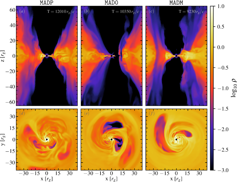
Figure 1: Flux tubes in the 3D GRMHD simulations visualized with meridial (panels $a$, $b$, $c$) and equatorial (panels $d$, $e$, $f$) slices. They correspond to low-density ($\rho$) and high-magnetization regions that come about after a magnetically-driven flux eruption starting from the central BH. The chosen slices correspond to promising time-lag windows, as listed in Table 4.

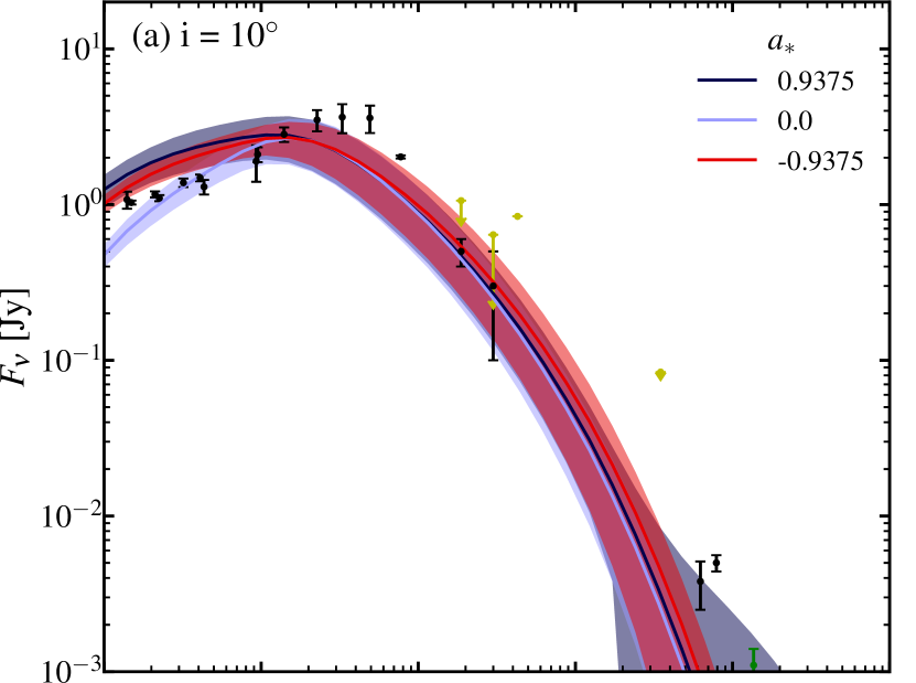
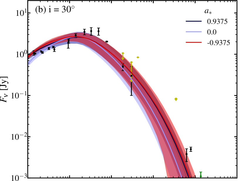
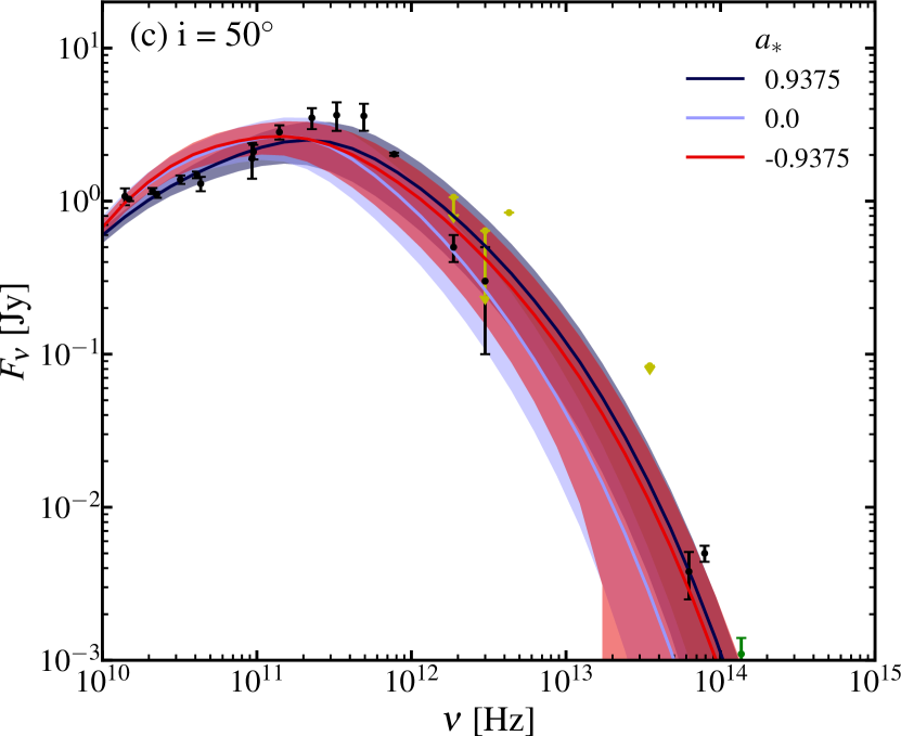
Figure 2: SEDs for three inclinations with $i=10^{\circ}$ (panel a), $i=30^{\circ}$ (b), and $i=50^{\circ}$ (c). Each panel contains the fit corresponding to the models MADP ($a_{\ast}=0.9375$), MAD0 ($a_{\ast}=0.0$), and MAD0 ($a_{\ast}=-0.9375$) where the shaded region denotes the one-sigma standard deviation for the $1$ $r_{\mathrm{g}}/c$ spaced lightcurves at each frequency. The origin of the observational points are listed in section 3.1.

2.1 General Relativistic MagnetoHydroDynamics

We simulate the accretion flow surrounding a rotating Kerr black hole with the Black Hole Accretion Code (BHAC, Porth et al., 2017; Olivares et al., 2019), which solves the MHD equations in a general-relativistic context. These equations are defined as;

$$\nabla_{\mu}(\rho u^{\mu})=0,$$ (1)

$$\nabla_{\mu}T^{\mu\nu}=0,$$ (2)

$$\nabla_{\mu}\tensor[^{\star}]{F}{{}^{\mu\nu}}=0,$$ (3)

where $\nabla_{\mu}$ denotes the covariant derivative, $\rho$ the rest-mass density, $u^{\mu}$ the fluid four-velocity, $T^{\mu\nu}$ the energy-momentum tensor (containing both ideal fluid and electromagnetic components), and $\tensor[^{\star}]{F}{{}^{\mu\nu}}$ the (Hodge) dual of the Faraday tensor. We assume an ideal MHD description, which implies that the electric field is acquired via the “frozen-in” condition (i.e., $\bm{E}=-\bm{v}\times\bm{B}$).

Our 3D simulations investigate three black hole spins, $a_{\ast}=-0.9375,0.0,0.9375$, which will be referred to as MADM, MAD0, and MADP. The simulations were performed using Modified Kerr-Schild coordinates (MKS, McKinney et al., 2012), which are logarithmically spaced in the radial direction and concentrates resolution in the equatorial plane (with $h=0.25$ and $R=0$, see Eqs. 49 and 50 in Porth et al. 2017). Nevertheless, we will only list the following quantities using Kerr-Schild (KS) coordinates ($t$, $r$, $\theta$, $\phi$).

One of BHAC’s main features is the inherent Adaptive-Mesh-Refinement (AMR) construction of the underlying grid – refine- and derefinement of the grid is possible based on user-defined criterion. This allows for a more efficient resolution allocation and, therefore, increases computational performance. While resolution is typically concentrated in the disc region to ensure a well-resolved magneto-rotational instability (MRI), our simulations have an additional high refinement block on the jet-disc boundary. As is shown explicitly in Appendix C, these blocks are at the highest AMR level corresponding to the resolution level that is listed in Table 1, alongside other simulation parameters. Due to the logarithmic radial spacing of the grid, this is still at a lower effective resolution level than close to be BH. Another feature of our simulations is that it has a high output cadence of 1 $r_{\mathrm{g}}/c$, a factor 5-10 larger than comparable works, which makes it well-suited to conduct variability and ‘slow light’ studies (see both Sect. 2.5 and 3.4).

The simulations are initialized from a hydrostatic equilibrium solution (FM; Fishbone & Moncrief, 1976) with the main user-defined parameters and naming conventions being introduced in Table 1. The disc is seeded with a (perturbing) poloidal magnetic field that is initialized via the following vector potential;

$$A_{\phi}\propto\max\left(\rho\left(\frac{r}{r_{\rm in}}\right)^{3}\sin^{3}\theta\exp\left(-\frac{r}{400}\right)-0.2,\>0\right).$$ (4)

Here, $\rho$ and $r_{\mathrm{in}}$ denote the density and inner radius of the torus at initialization. The resulting, evolved magnetic field brings about the MAD state which is characterized by magnetic flux eruption that locally and temporarily halt the accretion flow onto the black hole as demonstrated in Fig. 1. These flux eruption come about when the black hole saturates in horizon-penetrating magnetic flux after which the flux eruption generates a vertical magnetic field that creates a barrier and halts the accretion flow. The resulting under-dense, over-magnetized regions are dubbed flux tubes (McKinney et al., 2012; Dexter et al., 2020; Porth et al., 2021), as outlined in the Introduction.

Table 1: Overview of GRMHD simulations.

Model	Spin	Eff. Resolution	$r_{\mathrm{in}}$	$r_{\rho_{\mathrm{max}}}$
Name	$a_{*}$	$N_{r}$, $N_{\theta}$, $N_{\phi}$
MADP	0.9375	768,384,384	20	41
MAD0	0.0	768,384,384	20	41
MADM	-0.9375	768,384,384	20	42

2.2 Radiative transfer

To obtain synthetic images, lightcurves, and spectra, we post-process our GRMHD simulations with the general-relativistic radiative-transfer code RAPTOR (Bronzwaer et al., 2018, 2020), which computes null-geodesics along which the radiative transfer equations are solved assuming thermal synchrotron emission (according to Leung et al. 2011). It is currently the only code that supports a direct readout of the native non-uniform AMR data structure as generated by BHAC (Davelaar et al., 2019). After the null-geodesics are calculated, we infer the electron temperature via a coupling relation as we are only evolving a (proton) one-fluid. We utilize the so-called R$\beta$ description (Mościbrodzka et al., 2016) that allows for a parametrization of the ion-to-electron temperature ratio ($T_{\mathrm{ratio}}$) as a function of the local plasma $\beta$ (ratio of gas to magnetic pressure) from which one then acquires the dimensionless electron temperature ($\Theta_{e}$) according to;

$$T_{\text{ratio}}=\frac{T_{p}}{T_{e}}=R_{\text{low}}\frac{1}{1+\beta^{2}}+R_{\text{high}}\frac{\beta^{2}}{1+\beta^{2}},\\$$ (5)

$$\Theta_{e}=\frac{U\,(\hat{\gamma}-1)\,m_{p}/m_{e}}{\rho\,(T_{\text{ratio}}+1)}.$$ (6)

Hereto undefined quantities are plasma $\beta=2p/B^{2}$, internal energy density ($U$), proton mass ($m_{p}$) and electron mass ($m_{e}$). In this work, we will exclusively image our models with $R_{\mathrm{high}}=100$ and $R_{\mathrm{low}}=1$, where $R_{\mathrm{low}}$ is almost exclusively and $R_{\mathrm{high}}$ This is effectively because a high $R_{\mathrm{high}}$ corresponds to relatively hot jet/jet-sheath electrons and relatively cool disc electrons, while for low $R_{\mathrm{high}}$ the electron temperature is more uniform. We look at the accretion system under three inclinations angles $i=10^{\circ},30^{\circ},50^{\circ}$. Our choices in $R_{\mathrm{high}}$ as well as inclinations are consistent with promising regions of the parameter-space as explored in EHTC et al. (2022a). We will evaluate the lightcurves and/or images at frequencies $\nu\in\{19,21,23,25,30,32,34,36,41,43,45,47\}$ GHz (following BR21, ). To appropriately cover the large-scale emission features present at these radio-wavelengths, we have utilized a spherical polar camera grid where the pixels are spaced logarithmically in the radial direction (outlined in Davelaar et al., 2018) with a resolution of $256\times 256$ pixels, which has been shown to converge with results at higher resolutions (Davelaar et al., 2018), and a radial size of 500 $r_{\mathrm{g}}$. As regions in the inner jet-funnel tend to be dominated by emission from floor-violations, one has to exclude these from the radiative transfer procedure. We employ both a geometrical and a standard (cold) magnetization criterion ($\sigma=B^{2}/\rho>1.0$) where we set the synchrotron emissivity to zero. For the geometrical cut, we assume a conical ($7.5^{\circ}$) cutout up to a radius $r=50$ $r_{\mathrm{g}}$ after which we utilize a staged cylindrical (with cylindrical radius $r_{c}$) cutout (i.e., [i] $r_{c}<10$ for $r\geqslant 50$, [ii] $r_{c}<25$ for $r\geqslant 300$).

Lastly, we will introduce the relevant scaling relations. GRMHD simulations are naturally scale-invariant and it is therefore possible to scale it to any (RIAF) system. To scale our simulations we need to define a black hole mass ($M_{\mathrm{BH}}$), which sets the time and length units, and a user-defined parameter called the mass unit ($\mathcal{M}$) that sets the overall energy budget of the accretion flow. The total produced emission is also effectively set with $\mathcal{M}$ and this parameter is therefore varied until one acquires the desired integrated emission level. We will predominantly be working with a theoretically advantageous unit-set that is based on gravitational radius $r_{\rm g}=GM/c^{2}$ and its time-unit $t_{g}=r_{g}/c$, which both reduce simply to $M$ in geometrized units $G=c=1$. The black hole mass is set to $M_{\mathrm{BH}}=4.1\times 10^{6}\,M_{\sun}$ in combination with a distance to the central black hole of $D=8.125$ kpc following Gravity Collaboration et al. (2018). Expressed in cgs units, we find that $t_{g}\approx 20.2$ s and the angular size correspond to a single $r_{g}$ is $\theta_{\rm g}=5\,\mu as$ (see also, e.g., EHTC et al., 2022b).

2.3 Local cross-correlation function and goodness-of-fit estimation

To compute the time-lags from our synthetic lightcurves we use the local cross-correlation function (Welsh, 1999; Max-Moerbeck et al., 2014). The LCCF enables cross-correlation between unevenly sampled timeseries and will be used exclusively to estimate the time-lags in this work. Even though the simulated lightcurves are evenly sampled by construction, we still utilize the LCCF as this is consistent with the methodology outlined in ; . We will cross-correlate all lightcurves with a reference $\nu_{1}$ = 19 GHz lightcurve, which implies that the auto-correlation will serve as the zeroth time-lag point.

To determine the similarity between the simulated ($E_{i,\mathrm{sim}}$) and observed time-lags ($O_{i,\mathrm{obs}}$), we evaluate the $\chi^{2}$ statistic for the six listed time-lags values (excluding 100 GHz) in BR15 to see which lightcurve sections are most similar to the observational equivalent. However, as the acquired time-lags can be arbitrarily shifted ($\xi$) in time, we minimise the following function to assess goodness of fit;

$$\chi^{2}=\sum_{i}^{N}\left[\frac{O_{i,\mathrm{obs}}-E_{i,\mathrm{sim}}-\xi}{\sigma_{i,\mathrm{obs}}}\right]^{2},$$ (7)

where $\sigma_{i,\mathrm{obs}}$ denotes the observational standard deviation and the sum is over the number of frequencies $N=12$. In addition to the goodness-of-fit estimation with the observations directly, we will calculated it also with respect to the linear fit from BR15 (with a slope of 42 min/cm) to gauge similarity to the preferred linear relation as expected from theory (Falcke et al., 2009). An overview of the best-fitting windows in outlined in Appendix D.

2.4 Favoured linear fit

In addition to assessing our ability to recover the observational time-lags, we will ascertain the preferred linear time-lag relation for the evaluated simulations. As, from isotropic outflow arguments, a linear relation is expected in the case of a relatively simplistic conical jet structure (Falcke et al., 2009), this is an interesting test to find the deviations from this picture. So, more specifically, we will fit a linear relation ($y=Ax+B$) to all time-lags acquired from the simulations and assess the root-mean-square error (RMSE) to evaluate goodness-of-fit according to;

$$\mathrm{RMSE}=\sqrt{\frac{1}{N}\sum_{i=1}^{N}\left(T-T_{\mathrm{f}}\right)^{2}}.$$ (8)

Here, $T$ is the simulation time-lag and $T_{\mathrm{f}}$ is the time-lag prescribed by the fit at the (N=)12 frequencies evaluated in this work. Typically, one finds errors of $\mathrm{RMSE}\lesssim 5$ for time-lag windows that show a fairly linear relation.

2.5 Slow light: basic implementation

The fast- vs. slow-light paradigm is quite well-investigated for mm-wavelength emission originating from close to the BH (see, e.g., Dexter et al., 2010; Bronzwaer et al., 2018; Mościbrodzka et al., 2021). For ray-tracing GRMHD simulations the standard in the field is to use a ‘fast light’ prescription, which entails that the plasma description is not evolved while the radiative transfer equations are evaluated along the null-geodesics. This effectively renders the speed of light to be infinite. For a more realistic description, denoted as ‘slow light’, one needs to evolve the plasma and light simultaneously. Overall, one can identify two scenarios where a slow-light prescription could make a significant difference. First, when one experiences strong space-time curvature, which is important for emission originating predominantly from within the inner $5-10$ $r_{\mathrm{g}}$. Even though matter moves fast ($v\cong 0.5c$) for this scenario, relatively few photons escape from innermost accretion regions and the time-lags are relatively when they originate close to the BH, which is partly explained by the confined region in which they are created. Second, when matter is moving (relatively) fast over long distances, which one associates with emission from the jet(-sheath). Contrary to all previously mentioned studies at $230$ GHz (1.3 mm), our scenario falls within the second category which is the more complicated case as we will outline in the following paragraph.

The complexity of this latter case lies predominantly with the large and diffuse emission structure as is present for the 19 GHz images in this work. So, when the emission structure is compact (at, e.g., 230 GHz), then one only has to read in relatively few slices to get a consistent picture. Our convergence study indicates that slow-light images at this frequency converge starting from $\sim$550 GRMHD snapshots assuming a 1 $r_{\mathrm{g}}/c$ cadence – reading in more would only results in minor $\mathcal{O}(0.5\%)$ image morphology differences at places with significant emission. Therefore, to be on the conservative side, we have opted for read-in GRMHD snapshot count of 600 per slow light image. Naturally, the convergence number is determined by when one reaches the limiting optical depth of $\tau\gtrsim 1$ after which the medium becomes (too) optically thick and (almost) no increase in emission occurs. This is the case for all radiative transfer studies, only for ‘slow light’ this limiting surface is dependent on the plasma conditions over a given time.

In practice, we employ a hybrid slow and fast light approach, where we calibrate the ‘slow light’ integration region along the geodesic so that (almost) all emission is described in the slow light window. As mentioned, for this ‘slow light’ implementation, we read-in 600 GRMHD files ($\sim$350 GB) that will give the plasma description at different times along the geodesic and it is therefore a memory-intensive procedure. The implementation relies on two dependent parameters; $r_{\mathrm{slow}}$ and $N_{\mathrm{snap}}$, while the latter denotes how many GRMHD snapshots are read in, the former determines from what time-coordinate along the ray the slow light description is assumed. As the geodesics are integrated backwards, the GRMHD description starts to move back in time until it has reached $T_{\mathrm{END}}=T_{\mathrm{START}}-N_{\mathrm{snap}}$. All integration before $T_{\mathrm{START}}$ and after $T_{\mathrm{END}}$ assumes fast light. For this approach, one has to calibrate for $N_{\mathrm{snap}}$ and find the number after which difference in emission structure are at an acceptable level. In this work, we choose to include a study of the most prominent ‘fast light’ time window, as we investigate a scenario where the inclusion of ‘slow light’ could have a significant effect (Sect. 3.4).

3 Results

In the following sections, we discuss the fitted spectra (Sect. 3.1), the qualitative (Sect. 3.2) and quantitative (Sect. 3.3) aspects of the time-lag analysis, and the implications of adopting a slow light approach (Sect. 3.4).

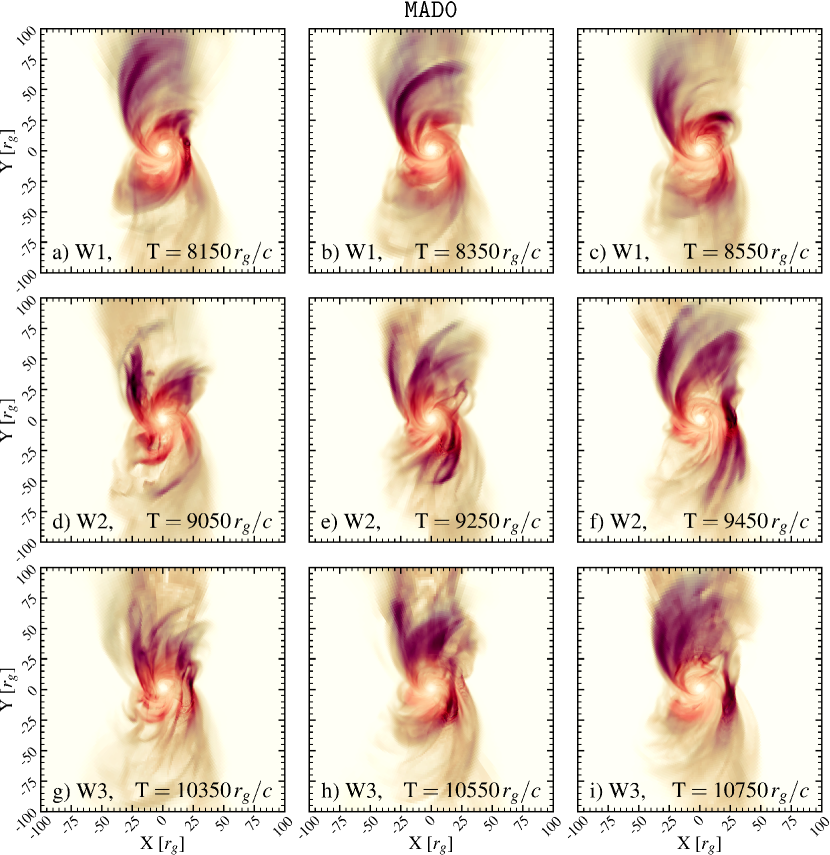
Figure 3: Ray-traced images for an inclination $i=30^{\circ}$ that consist of three combined colormaps corresponding to the thermal synchrotron emission at $\nu=19,\,32,\,\mathrm{and}\>47$ GHz in shades of green-blue, red-purple, and orange-red, respectively. When emission from all frequencies is present, one creates a black-purple hue in the composite image. All base image maps describe the flux density ($F_{\nu}$) between $0.0$ and $0.025$ Jy per pixel. The base images are combined with equal weight to acquire the composite images. More details on the procedure as well as animations for all cases are provided in Appendix A.

3.1 Spectral Energy Distributions

Figure 2 displays the Spectral Energy Distributions (SEDs) for all our ray-traced models. The spectra were fitted with a binary search algorithm (also utilized and outlined in Bronzwaer et al., 2021) which launches the ray-tracing code in an iterative manner and fits the 230 GHz flux density $F_{\nu}$ to $2.5\pm 0.03$ Jy. With this relatively simple procedure and an exclusively thermal electron population, we obtain good fits to the quiescent Sgr A^∗ spectrum at inclinations of $i=10^{\circ}$, $30^{\circ}$, and $50^{\circ}$. Especially for $i=30^{\circ}$ and $i=50^{\circ}$, we obtain SEDs that correspond well to the binned observational data that are gathered from Falcke et al. (1998); Schödel et al. (2011); Bower et al. (2015, 2019); Witzel et al. (2018); von Fellenberg et al. (2018); Gravity Collaboration et al. (2020). At $i=10^{\circ}$, we tend to either under- or overproduce the radio emission ($\nu\lesssim 100$ GHz).

For our fits we find a corresponding accretion rate via $\dot{M}_{\mathrm{cgs}}=\mathcal{M}\cdot\langle\dot{M}_{\mathrm{sim}}\rangle/t_{\mathrm{g}}$, where the simulation accretion rate ($\dot{M}_{\mathrm{sim}}$) is the averaged over the evaluated time-domain (i.e., $T\in[6300,15300]\,r_{\mathrm{g}}/c$). For inclination $i=30^{\circ}$, we find accretion rates of $\dot{M}_{\mathrm{cgs}}=5.69\times 10^{-9},1.52\times 10^{-8},1.62\times 10^{-8}\,M_{\sun}/\mathrm{yr}$ for MADP, MAD0, and MADM, respectively. As $\mathcal{M}$ is calculated for every inclination (and simulation) separately, the accretion rate will vary quite substantially, but remains low as is outlined in Appendix B. We list the $i=30^{\circ}$ accretion rates explicitly as they correspond to the favoured models in this work.

3.2 Qualitative analysis of Time-lags

Figure 3 displays composite ray-traced images of thermal synchrotron emission at $19$ (blue-green), $32$ (pink-purple), and $47$ GHz (red-orange) for selected windows of the MAD0 case. This allows for an intuitive interpretation of how emission features move through frequency space, where dark regions indicate coincident emission at all frequencies. As time-lags move from high to low frequencies, it will start out as a red hue and gradually move to blue/purple and end in black. Window 2 (W2, in panels $d$,$e$,$f$) gives a prime example of this behavior, especially if one looks at the flux tube that starts out with a red color and gradually becomes darker as it cools.

Figures 4, 5, and 6 consist of the corresponding lightcurves and display LCCF coefficients of three sections of the lightcurves (W1, W2, and W3) for the MADP, MAD0, and MADM cases, respectively. The classical interpretation of the time-lags rests on the frequency-dependent synchrotron emission from a (mildly-)relativistic, conical jet (see, e.g., Blandford & Königl, 1979; Falcke et al., 1993; Falcke & Biermann, 1999; Falcke et al., 2009), or even an expanding blob of plasma (van der Laan, 1966). Even though the jet picture is broadly correct, it is not sufficient to explain the time-lags from our simulations. As these are relatively short observing windows (of up to $400\,r_{g}/c\approx 2.25\,\mathrm{hrs}$), the variable emission component is arguably more important than the relatively static jet emission structure, which is confirmed by our findings. More specifically, we note that a number of windows (in Figures 4, 5, and 6) containing good time-lag fits follow closely after a flux eruption event which is denoted by the drop in $\Phi_{\mathrm{B}}$ (magenta line), as will be explained in more detail in next paragraph(s).

We postulate that the main driver behind the variable component in our MAD simulation is the formation of flux tubes after a magnetic flux eruptions. During these flux eruptions, a low-density, high-magnetization region is created after the BH saturates in horizon-penetrating magnetic flux ($\Phi_{\mathrm{B}}$; Tchekhovskoy et al., 2011). When this occurs, a part of the magnetic flux $\Phi_{\mathrm{B}}$ is dissipated by means of a magnetic reconnection event that generated a strong vertical magnetic field component which partly halts and pushes back the accretion flow effectively creating the flux tube. The flux tube is aligned with the jet and orbits the BH at sub-Keplerian velocities before expanding and eventually dissipating into the disc. This can span several orbital periods ($\sim 1500$ $r_{\mathrm{g}}/c$ for, e.g., W2 in Fig. 5). At its birth, it is predominantly visible in the higher frequency emission (red) before it expands and cools so it will start emitting at lower frequencies also (creating the purple-black hue).

Interestingly, as it matures, the tail-end of the flux tube (furthest away from the BH) produces the strongest emission feature as the flux tube is pushing against the accretion flow which compresses (creating an over-density) and heats the electrons as is clearly shown in Appendix C (also commented on in Najafi-Ziyazi et al., 2023). This emission feature has the resemblance of a ‘hot spot’ (Broderick & Loeb, 2006; Vos et al., 2022), especially when the flux tube is receding with respect to the observer as one then directly looks at (the back of) the compression region. We note that this deviates in interpretation from the standard hot spot model as the point of maximal emission typically occurs when the spot approaches the observer and is maximally (Doppler) beamed (cf. Vos et al., 2022). For $i=50^{\circ}$, however, one clearly sees a vertical tube emission structure, which is quite different from the typical spherical hot spot picture. Another channel by which variable emission features originate is the non-homogeneous nature of the jet sheath (or wall), which produces the majority of the emission overall. Over-dense outflows will occur sporadically and are sheared and subsequently ‘smeared’ out over the jet sheath cone. Nevertheless, we find that the jet-sheath-related bursts in emission are often closely preceded by a flux eruption event, so even though they originate is different parts of the simulation domain they are triggered by the same physical mechanism.

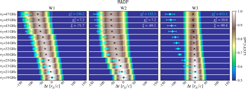
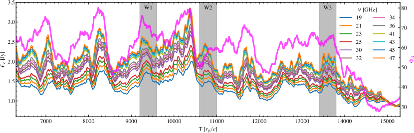
Figure 4: LCCF coefficients and lightcurves for the MADP case at $i=30^{\circ}$. For the LCCF (in the top panel), we choose one lightcurve ($\nu_{1}=19$ GHz) that we cross-correlate with all other lightcurves ($\nu_{2}$). The black crosses (‘x’) denotes the maximum of the LCCF within a given window. The cyan diamants with errors denote the fit obtained in BR15. Both the lightcurves, ranging from $19$ to $47$ GHz, and horizon-penetrating magnetic flux $\Phi_{B}$ are shown in the bottom panel. The three windows W1, W2, and W3 are $400$ $r_{\mathrm{g}}/c$ in length and correspond to the LCCF panels shown in the top.

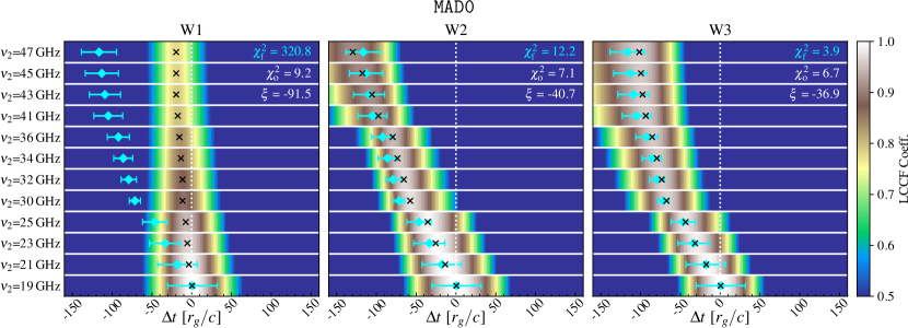
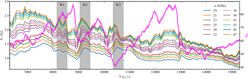
Figure 5: LCCF coefficients and lightcurves for the MAD0 case at $i=30^{\circ}$. The rest of the description of Fig. 4 is also applicable here.

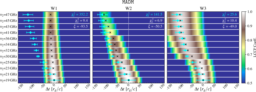
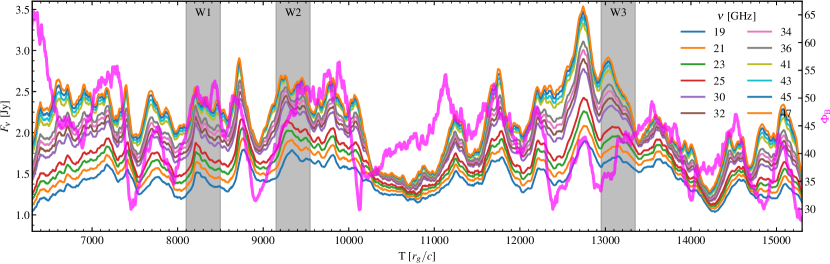
Figure 6: LCCF coefficients and lightcurves for the MADM case at $i=30^{\circ}$. The rest of the description of Fig. 4 is also applicable here.

3.3 Quantitative analysis of Time-lags

Presently, we have identified several channels via which time-lags can be created. To quantify how well our simulations agree with the findings of ; , we calculate the time-lags over sections of the synthetic lightcurves for time windows of 100, 200, 300, and 400 $r_{\mathrm{g}}/c$. The window is shifted with steps of 10 $r_{\mathrm{g}}/c$ until the entire lightcurve is covered. The acquired time-lags are then scored with two types of $\chi^{2}$ estimate. Following the method outlined in Sect. 2.3, we calculate $\chi^{2}_{\mathrm{o}}$ directly with the observations. Then, we calculate $\chi^{2}_{\mathrm{f}}$ between the linear fits listed in BR15 and our simulated ones to get an idication if we are able to recover this slope. The overview table (4) is listed in Appendix D. We note that the 25 GHz measurement (from Brinkerink et al., 2015) deviates significantly from the otherwise linear trend in the data and is therefore not well-represented in the linear fit. We also investigate the preferred linear relations from our simulated data which will be outlined later in this section. Overall, the $\chi^{2}_{\mathrm{o}}$ is significantly less constraining than $\chi^{2}_{\mathrm{f}}$ as a result of the large errors on the observational time-lags. Nevertheless, the combined constrains (both $\chi^{2}<7$) are restricting, but still identify a number of passing windows with a preference for the MAD0 case, especially with $i=30^{\circ}/50^{\circ}$ and longer correlation windows. The choice for $\chi^{2}<7$ is arbitrary and quite stringent, but it also clearly highlights windows where the simulation’s behavior is highly consistent with BR15, as we find a reduced $\chi^{2}_{\nu}\lesssim 1.2$ (for the six observational points in the case of $\chi^{2}_{\mathrm{o}}$ and 12 for $\chi^{2}_{\mathrm{f}}$ as shown in, e.g., Fig. 4).

The physical manifestation of the best-fitting time-lags corresponds to a flux tube that starts directly in front of the main jet structure and continues it’s counter-clockwise trajectory till it moves behind the jet. Even behind the jet, the flux tubes still contributes to the observed flux. As clearly seen in W2 and W3 of Fig. 3, the flux eruption that creates the flux tube also give an increase in the high frequency (red) emission that will gradually move to lower frequencies in the jet sheath (dark purple). The time-lag displays quite an characteristic kink in the low frequency bands to accommodate for the outlier (at 25 GHz). The largest passing window is denoted by W3 in both Figs. 3 and 5. For completeness, we note the data listed in BR21 is more complex in nature than what was used for BR15 but is still consistent with the linear relation that we investigate (i.e., $\chi^{2}_{\mathrm{f}}$ in Table 4).

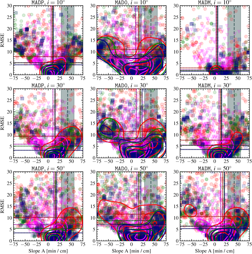
Figure 7: RMSE of calculated simulations time-lags with respect to their linear fit. The points are color-coded according to the time-lag window lenght; 100 (magenta), 200 (red), 300 (green), and 400 (blue) $r_{\mathrm{g}}/c$. The color-dashed lines denote the mean slope of the best-fitting (RMSE ¡ 5) time-lags for the vertical lines, while the horizontal lines denote the mean RMSE of the entire population. The grey dashed line, with standard deviation area, corresponds to the linear fit to the VLA-only data from BR15, which is $A=42\pm 14$ cm/min. The contours denote the $25\%$, $50\%$, and $75\%$ levels of the normalized kernel density estimations for each of the window length results (in the corresponding colors).

Figure 7 answers two main questions; how linear are the simulation time-lag relations and which slope would best fit them? While all distributions display considerable variance, we note that one finds quite a considerable number of points in the area corresponding to the fit of BR15 in the grey shaded area; $A=41\pm 14$ cm/min. The mean slope of the best-fitting time-lag distributions (denoted by the black-color dashed vertical lines) are significantly lower than the observational slope. This indicates that most linear time-lags from the simulations favour a more shallow slope than was found for BR15 and/or the steeper better-fitting time-lags favour do not display linear behavior. Therefore, based on the results from this work, we find that the relatively steep slope is a rare occurrence according to our simulations. A last point to consider is that a significant portion of observational time-lags do not show a clear relation (BR21). Interestingly, this behavior is also recovered for our idealized simulations as they do regularly not show a clear time-lag relation (i.e. there are breaks or multiple competing features in the LCCF coeff.), as is indicated by the black-color dashed horizontal lines that denotes the mean RMSE of all points. This indicates that a time-lag analysis is typically difficult, but there are indications that longer LCCF windows improve linearity in the time-lags. Overall, based on the kernel density contours, we find that most of the simulated time-lags show are predominantly linear ($\mathrm{RMSE}<5$) trend which is typically lower than $A=41\pm 14$ cm/min. The linear trend that is preferred from simulations is $A\in[7,23]$ cm/min based on the $400$ window length calculations, with $A\approx 20$ cm/min for MAD0 and lower values for MADP and MADM which increase with inclination from $A\approx 10$ cm/min at $i=10^{\circ}$ to $A\approx 20$ cm/min at $i=50^{\circ}$.

3.4 Slow light comparison

After one has acquired the slow lightcurve, it is beneficial to find the optimal offset between both the fast and slow lightcurves, which allows for more intuitive comparison. However, this is a somewhat non-trivial procedure as the timing between various features differs depending on your light description. While one has several options to find the offset (e.g., via cross-correlation of either the images or the ligthcurves), we have have opted for the minimisation of the Euclidean distance between segments of the slow and fast light curves (i.e., 1D trivial equivalent of the down-hill-simplex method; Press et al. 2002). Taking $\nu=19$ GHz as the reference frequency, we find an offset in time of $\Delta t=365$ $r_{\mathrm{g}}/c$, while for $\nu=47$ GHz we find $\Delta t=402$ $r_{\mathrm{g}}/c$. Nevertheless, we would like to note that for the outcome of the LCCF calculations the alignment shift is inconsequential as one calculates the time-lags between the various frequency lightcurves within their corresponding groups.

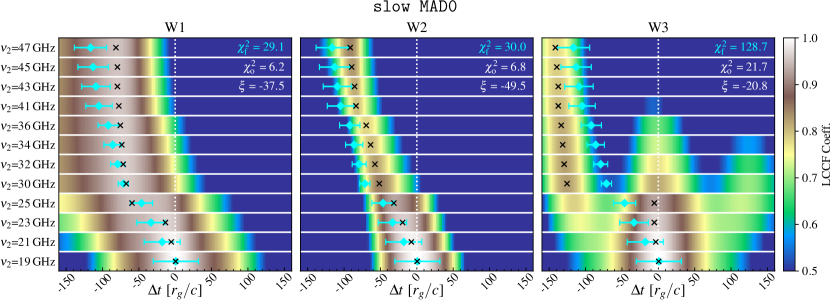
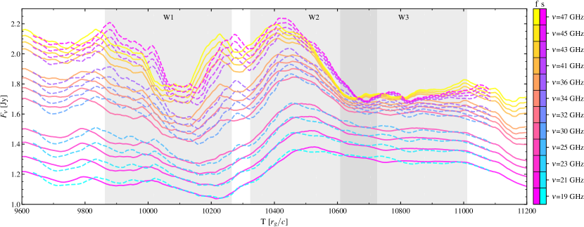
Figure 8: Fast and slow lightcurves for the MAD0 case at $i=30^{\circ}$. The slow light window was chosen to correspond to the most promising time-lag window for the fast light curves, as indicated by Table 4. The color-schemes corresponding to the various frequencies for the fast (solid) and slow (dashed lines) lightcurves are denoted by the ‘f’ and ‘s’, respectively. The three windows W1, W2, and W3 are 400 $r_{\mathrm{g}}/c$ in length and correspond to the LCCF panels shown at the top, analogously to Fig. 5 for fast light.

Figure 8 displays the fast and slow lightcurves corresponding to the promising window centered around $T=10400$ $r_{\mathrm{g}}/c$ for the MAD0, $i=30^{\circ}$ case. What becomes clear is that the slow light description has strong consequences for the resulting time-lags. We only calculate the alignment shift for $\nu=19$ GHz and shift all slow light curves accordingly. As we expected, timing between various features has changed significantly resulting in a seemingly worse correspondence with the observational time-lags (especially for $\chi^{2}_{\mathrm{f}}$ as listed in Table 4). This is also reflected in the time-lag panels in the top of Fig. 8. Nevertheless, what has not changed is that a relatively large number of time-lags pass the $\chi^{2}_{\mathrm{o}}$ constraint. For the $\chi^{2}_{\mathrm{f}}$ constraint, however, we find that almost no time-lag passes. This indicates that while there is a good consistency when the time-lag is compared to the observational data directly it is not consistent with the proposed linear fit. The slow lightcurves show a preference for shallower slopes. More specifically, W2 in Fig. 8 corresponds almost exactly to the same window shown in Fig. 5. While we find a similar $\chi^{2}_{\mathrm{o}}\approx 7$, we find that $\chi^{2}_{\mathrm{f}}$ differs significantly, which highlights the sensitivity of this particular diagnostic.

To conclude, we will comment on why the slow light time-lags seem to fit less well to the observational time-lag than the fast light counterpart. Employing the simplest interpretation, there are two main ways in which the lightcurves change when comparing fast with slow light, namely the timing between features differs or the features are different themselves. While the former point is largely determined by relative emission structure sizes and the associated light travel time difference, the latter point is associated with the radiative transfer calculations itself. The preferred shallower slope does indicate a change in timing and from the lightcurves we can already ascertain the more peaky nature of the slow light curves. For the slow light approach, one expects to find differences in regions where the plasma moves with or against the (integration) direction of the light rays, which either results in increased or reduced emission, respectively. Another clear affect is found in the size of the emission structure, which is smaller for the higher frequencies indicating longer light travel times. The higher the velocity of plasma, the greater this effect will be. From this preliminary study, it becomes clear that the adaption of a slow light approach is able to significantly alter lightcurves and underlying images at the evaluated wavelengths, and does not necessarily result in better correspondence to the observational time-lags (for the evaluated window).

4 Discussion and Conclusion

We have demonstrated that flux eruption events and the emergence of flux tubes are consequential for the emission features at radio frequencies ($\nu=19-47$ GHz). Selected windows from our simulations are well-able to reproduce the characteristic observational time-lag as presented in ; . Interestingly, flux tube emission is prominently featured in the best-fitting time-lag windows, but that does not mean that the classical picture with an expanding and cooling jet sheath is no longer applicable. We advocate a more complex picture where the flux eruption, subsequent flux tube, and jet sheath are all affecting and perturbing one another, which is clearly seen in the most promising windows (in Fig. 3). The question what happens to these features at larger distances sill remains open. As our simulations display strong outflows extending several hundreds of $r_{\mathrm{g}}$, one wonders about the exact origin of VLBI jet (Lobanov & Zensus, 1999; Kim et al., 2023) observations which could perhaps be explained with a strong outflow starting at the central black hole rather than the collimation shock picture. However, we also note that our modelling only deals within the inner 500 $r_{\mathrm{g}}$ and that these VLBI jet observation span several thousands of $r_{\mathrm{g}}$.

A number of effects, that were not within the scope of this work, are likely to influence our results. To improve, one can consider the addition of non-thermal emission (Özel et al., 2000; Chan et al., 2009; Chael et al., 2017; Davelaar et al., 2018), GRMHD simulation focusing on better resolving the jet sheath (as seen in, e.g., Ripperda et al., 2022), and more elaborate electron heating prescriptions (see, e.g., Howes, 2010; Rowan et al., 2017, 2019; Kawazura et al., 2019) or even a more in-depth R$\beta$ study. Other possibilities that could have an effect on inclusion of non-ideal current sheets in the vicinity of the jet-disc interface (Ripperda et al., 2020; Vos et al., 2023). Additionally, polarised lightcurves (see, e.g., Najafi-Ziyazi et al., 2023; Davelaar et al., 2023) are likely to shed more light on the preferred magnetic field orientation and if it diverges significantly from the commonly applied singular poloidal loop, as outlined in section 2.1.

In this work, we have also undertaken an exploratory study to establish the sensitivity of our results to the ‘fast-light’ assumption and found that this does indeed have a significant effect on the outcome (see Sect. 3.4). Nevertheless, at face value, the slow light time-lags did not correspond better to the observational results, which high-lights that the fast vs. slow light paradigm is not intuitively understood, especially for a timing-sensitive study. Nevertheless, we have demonstrated that it is possible to explain the observed time-lags around Sgr A^∗ utilizing the modelling techniques outlined in this works.

Appendix A Animations

To display the time-lag in a visually intuitive manner, we combine images at multiple frequencies into a single multi-frequency image, from which one can intuitively interpret regions of simultaneous emission or when a feature is predominantly present at a single frequency. The colors per frequency are as follows: green-blue for $\nu=19$ GHz, pink-purple for $\nu=32$ GHz, orange-red for $\nu=47$ GHz that combine into a red to dark-purple/black master color scheme. All images saturate at a flux density ($F_{\nu}$) per pixel of $0.025$, which allows for interpreting which image feature (at which frequency) is most dominant. As we modify the RGBA codes of the base figures to acquire the top figure, one potentially loses some physical interpretability but one visual interpretation of the time-lag becomes more intuitive. The interpretation of the strongest emission features is naturally still robust. An example of how the combination of base images occurs is shown in Fig. 9.

As mentioned, all simulations have accompanying animations that are available in the following online repository; https://doi.org/10.5281/zenodo.10041492 .

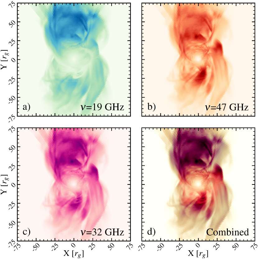
Figure 9: Schematic outlining the components of the multi-frequency graphics as shown in Fig. 3. The panels ($a$,$b$,$c$) display the flux density maps ($F_{\nu}$) at frequencies $\nu=19,32,47$ at $T=9230$ of the MADM, $i=30^{\circ}$ case, which is the same instance as shown in panels ($c$) and ($f$) of Fig. 1. The image’s RGBA codes are combined into the final result in the bottom right (panel $d$).

Appendix B Accretion rate for all simulations

Table 3 lists the acquired accretion rates as $\dot{M}_{\mathrm{cgs}}=\mathcal{M}\cdot\langle\dot{M}_{\mathrm{sim}}\rangle/t_{\mathrm{g}}$ as a function of the time-averaged simulation accretion rate ($\langle\dot{M}_{\mathrm{sim}}\rangle$) and the user-defined mass unit $\mathcal{M}$ as was outlined previously in Sect. 2.2 and 3.1. The flux calibration procedure, which we will outline in more detail here, is based on incrementally changing $\mathcal{M}$ based on the average flux acquired from a $100$ $r_{\mathrm{g}}/c$ spaced lightcurve. After updating $\mathcal{M}$, RAPTOR is launched 900 times as the total length of the lightcurve is $9000$ $r_{\mathrm{g}}/c$. The $\mathcal{M}$ space is sampled by means of a binary search and typically converges on the desired flux density ($F_{\nu}=2.5$ Jy at 230 GHz) in ten cycles or less.

Table 2: Accretion rates for all GRMHD simulations.

Model	$i$	$\mathcal{M}$	$\dot{M}_{\mathrm{cgs}}$
Name		[c.u.]	[$M_{\odot}$/yr]
MADP	$10^{\circ}$	$4.056742\times 10^{17}$	$5.522208\times 10^{-9}$
	$30^{\circ}$	$4.177095\times 10^{17}$	$5.686037\times 10^{-9}$
	$50^{\circ}$	$4.177095\times 10^{17}$	$5.686037\times 10^{-9}$
MAD0	$10^{\circ}$	$9.684549\times 10^{17}$	$1.636448\times 10^{-8}$
	$30^{\circ}$	$9.024831\times 10^{17}$	$1.524972\times 10^{-8}$
	$50^{\circ}$	$8.126574\times 10^{17}$	$1.373189\times 10^{-8}$
MADM	$10^{\circ}$	$7.225904\times 10^{17}$	$1.682900\times 10^{-8}$
	$30^{\circ}$	$6.943015\times 10^{17}$	$1.617016\times 10^{-8}$
	$50^{\circ}$	$6.378044\times 10^{17}$	$1.485435\times 10^{-8}$

Appendix C Grid layout of the GRMHD simulations and flux tube temperature profiles

Figure 10 displays the AMR grid layout of our simulations, with a high refinement block covering the jet-disc boundary, and gives insight into the temperature profile of the flux tubes. The high refinement blocks allow for capturing structural variability in the jet sheath better than is standardly applied. As it’s typically advantageous to keep the blocks at lowest level along the jet axis, we opted for the user-defined and intricate refinement scheme. Nevertheless, to sufficiently resolve plasma-driven (i.e. Kelvin-Helmholtz instabilities; Sironi et al. 2021) or even current-driven (i.e. magnetic reconnection; Ripperda et al. 2020; Vos et al. 2023) instabilities one needs much higher resolution levels to resolve these properly. Additionally, as discussed in Sect. 3.2, we find that tail-end of the flux tube is both heated and over-dense which gives it a clear emission feature, while the very center of the tube (having low density) is typically excluded from the GRRT analysis (as $\sigma>1$).

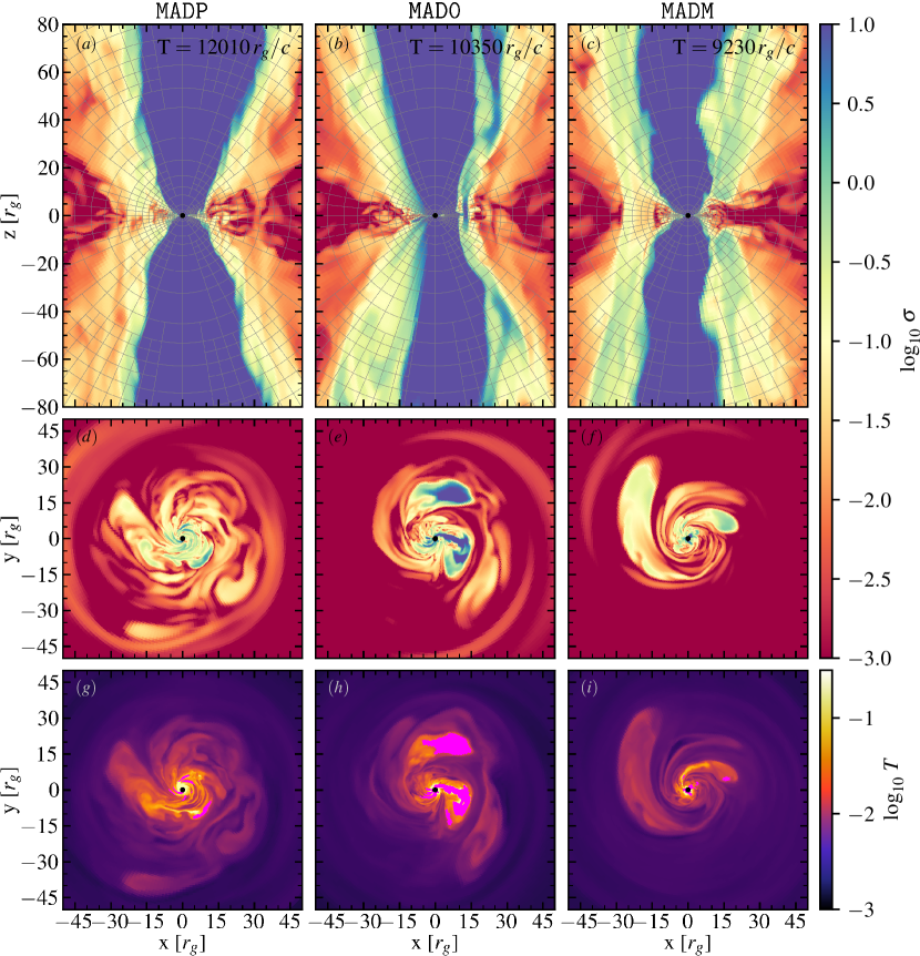
Figure 10: Flux tubes in the 3D GRMHD simulations visualized with meridial (panels $a$, $b$, $c$) and equatorial (panels $d$ till $i$) slices. Here, in addition to Fig. 1, we display (cold) magnetization $\sigma=B^{2}/\rho$ (panels $a$ till $f$) with the AMR structure (in grey) and temperature $T=p/\rho$ (panels $g$ till $i$). Each AMR block contains $8\times 8$ cells. For intuitive comparison with the GRRT images, we display $T$ regions with $\sigma>1$ in magenta as the emissivity is set to zero there. As mentioned, the chosen slices correspond to promising time-lag windows, as listed in Table 4.

Appendix D Best fit time-windows

Table 4 lists the time-windows of the simulated time-lags that fit best to the relation found in BR15. These windows are identified by means of $\chi^{2}_{\mathrm{f}}$ (related to the linear fit with slope $A=40\pm 14$ cm/min) or $\chi^{2}_{\mathrm{o}}$ (direct comparison with the six observational time-lags). The main identification criteria ($\chi^{2}_{\mathrm{x}}<7$, $\mathrm{x}\in[\mathrm{o},\mathrm{f}]$) are stringent, which ensure that we only identify the very best-fitting time-windows. We note that the reduced chi-squared, $\chi^{2}_{\nu}$, corresponding to the aforementioned criteria are $\chi^{2}_{\nu,\mathrm{o}}=1.17$ and $\chi^{2}_{\nu,\mathrm{f}}=0.58$, which clearly outlines that the $\chi^{2}_{\mathrm{f}}$ criterion is the main decider for the best-fitting windows. This also explains the main trends shown in the Table, which we will briefly discuss now.

Generally, from all evaluated cases, MAD0 is best able to recover the desired time-lag, especially for inclination of $i=30^{\circ}$ and $i=50^{\circ}$. Overall, column (i) outlines that numerous lightcurve sections have passable correspondence to the observations, where the $i=10^{\circ}$ cases are slightly disfavoured (especially for MADP and MADM). Column (ii) is where the clear preference arises for the MAD0 case, as it seems that the other cases are less able to recover the needed slope which is also clearly seen for Fig. 7. Columns (iii) and (iv) further accentuate the previously discussed point, but are nevertheless useful to select the very best time-lag windows. Nevertheless, we note that the $\chi^{2}_{\mathrm{o}}<7$ criterion is leading as it is (most) free from any predefined assumption (i.e., linearity with a certain slope). From this result, we conclude that there are numerous windows that are consistent, but there are indications for a preferred medium inclination ($i=30^{\circ}/50^{\circ}$) and low BH-spin (MAD0).

Table 3: Best-fitting simulation windows.

Model	Incl.	LCCF win.	(i) ($\chi^{2}_{\mathrm{o}}<8$)	(ii) ($\chi^{2}_{\mathrm{f}}<8$)	(iii) ($\chi^{2}_{\mathrm{o}}<8$)	(iv) ($\chi^{2}_{\mathrm{o}}<7$)	Best
Name		[$r_{g}/c$]			& ($\chi^{2}_{\mathrm{f}}<25$)	& ($\chi^{2}_{\mathrm{f}}<7$)	window
MADP	10∘	100	121 [13.6%]	0 [0.0%]	0 [0.0%]	0 [0.0%]	-
	10∘	200	78 [8.9%]	0 [0.0%]	0 [0.0%]	0 [0.0%]	-
	10∘	300	116 [13.3%]	0 [0.0%]	0 [0.0%]	0 [0.0%]	-
	10∘	400	174 [20.2%]	0 [0.0%]	0 [0.0%]	0 [0.0%]	-
	30∘	100	198 [22.2%]	0 [0.0%]	3 [0.3%]	0 [0.0%]	-
	30∘	200	199 [22.6%]	4 [0.5%]	20 [2.3%]	2 [0.2%]	11810, 13180
	30∘	300	224 [25.7%]	0 [0.0%]	2 [0.2%]	0 [0.0%]	-
	30∘	400	245 [28.5%]	0 [0.0%]	0 [0.0%]	0 [0.0%]	-
	50∘	100	196 [22.0%]	0 [0.0%]	1 [0.1%]	0 [0.0%]	-
	50∘	200	217 [24.6%]	2 [0.2%]	5 [0.6%]	1 [0.1%]	12790
	50∘	300	252 [28.9%]	1 [0.1%]	10 [1.1%]	0 [0.0%]	-
	50∘	400	288 [33.4%]	7 [0.8%]	17 [2.0%]	0 [0.0%]	-
MAD0	10∘	100	180 [20.2%]	0 [0.0%]	4 [0.4%]	0 [0.0%]	-
	10∘	200	191 [21.7%]	1 [0.1%]	10 [1.1%]	0 [0.0%]	-
	10∘	300	191 [21.9%]	7 [0.8%]	26 [3.0%]	2 [0.2%]	9910 - 9920
	10∘	400	171 [19.9%]	19 [2.2%]	28 [3.3%]	3 [0.3%]	7920 - 7930, 10410
	30∘	100	197 [22.1%]	0 [0.0%]	6 [0.7%]	0 [0.0%]	-
	30∘	200	184 [20.9%]	6 [0.7%]	20 [2.3%]	2 [0.2%]	7560, 9130
	30∘	300	168 [19.3%]	14 [1.6%]	35 [4.0%]	6 [0.7%]	9910, 10330-10370
	30∘	400	196 [22.8%]	31 [3.6%]	55 [6.4%]	8 [0.9%]	10310-10360, 11270-11280
	50∘	100	238 [26.7%]	0 [0.0%]	6 [0.7%]	0 [0.0%]	-
	50∘	200	222 [25.2%]	8 [0.9%]	30 [3.4%]	2 [0.2%]	10350-10360
	50∘	300	235 [27.0%]	27 [3.1%]	47 [5.4%]	7 [0.8%]	9080-9090, 10350-10390
	50∘	400	267 [31.0%]	43 [5.0%]	61 [7.1%]	3 [0.3%]	9860, 10370-10380
slow	30∘	100	49 [18.1%]	0 [0.0%]	0 [0.0%]	0 [0.0%]	-
MAD0	30∘	200	69 [27.5%]	0 [0.0%]	8 [3.2%]	0 [0.0%]	-
	30∘	300	78 [33.8%]	0 [0.0%]	1 [0.4%]	0 [0.0%]	-
	30∘	400	93 [44.1%]	0 [0.0%]	0 [0.0%]	0 [0.0%]	-
MADM	10∘	100	74 [8.3%]	0 [0.0%]	1 [0.1%]	0 [0.0%]	-
	10∘	200	76 [8.6%]	0 [0.0%]	6 [0.7%]	0 [0.0%]	-
	10∘	300	85 [9.8%]	2 [0.2%]	16 [1.8%]	0 [0.0%]	-
	10∘	400	82 [9.5%]	5 [0.6%]	5 [0.6%]	0 [0.0%]	-
	30∘	100	162 [18.2%]	0 [0.0%]	2 [0.2%]	0 [0.0%]	-
	30∘	200	182 [20.7%]	1 [0.1%]	6 [0.7%]	0 [0.0%]	-
	30∘	300	184 [21.1%]	3 [0.3%]	2 [0.2%]	0 [0.0%]	-
	30∘	400	237 [27.5%]	0 [0.0%]	11 [1.3%]	0 [0.0%]	-
	50∘	100	224 [25.1%]	0 [0.0%]	5 [0.6%]	0 [0.0%]	-
	50∘	200	237 [26.9%]	1 [0.1%]	3 [0.3%]	0 [0.0%]	-
	50∘	300	310 [35.6%]	4 [0.5%]	22 [2.5%]	2 [0.2%]	9100-9110
	50∘	400	368 [42.7%]	11 [1.3%]	39 [4.5%]	6 [0.7%]	8990, 9010-9040, 14450

Appendix E Different reference frequency

We have exclusively reported results using the reference frequency $\nu_{1}=19$ GHz. Even though one typically finds very consistent time-lags when choosing a different reference frequency, it is still possible that the time-lag behaviour changes. Here, we show the differences in results when when using reference frequencies of $\nu_{1}$ of 32 GHz. As mentioned before, only the slope of the relation is important in this instance as one naturally gets a difference offset when changing reference frequency as this corresponds to the zeroth time-lag point. In essence, we will therefore be repeating the analysis outlined in Sect. 2.4 and 3.3 to estimate the effect the choice in reference frequency makes for the final interpretation of the time-lags.

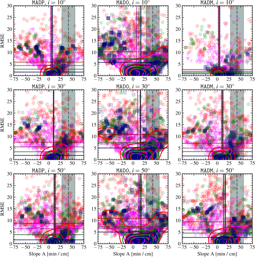
Figure 11: RMSE of calculated simulations time-lags with respect to their linear fit for a reference frequency of $\nu_{1}=32$ GHz. The points are color-coded according to the time-lag window lenght; 100 (magenta), 200 (red), 300 (green), and 400 (blue) $r_{\mathrm{g}}/c$. The color-dashed lines denote the mean slope of the best-fitting (RMSE ¡ 5) time-lags for the vertical lines, while the horizontal lines denote the mean RMSE of the entire population. The grey dashed line, with standard deviation area, corresponds to the linear fit to the VLA-only data from BR15, which is $A=42\pm 14$ cm/min. The contours denote the $25\%$, $50\%$, and $75\%$ levels of the normalized kernel density estimations for each of the window length results (in the corresponding colors). Figure 7 displays the results for a reference frequency of $\nu_{1}=19$ GHz, which was the base assumption throughout this work.

Based on the comparison of Fig. 11 ($\nu_{1}=32$ GHz) and Fig. 7 ($\nu_{1}=19$ GHz), we conclude that there are difference, which are best pointed out by the density contours, between both time-lag distributions, but the overall they agree well. Overall, the variation in the distribution itself is lower (i.e., density contours are more confined) and the best-fitting linear slopes ($\mathrm{RMSE}<5$) are slightly lower than what was found for $\nu_{1}=19$ GHz. Nevertheless, we still find a good number of time-lag slopes that lie within the shaded region. In our experience, when the reference lightcurve is smooth or devoid of small-scale features, it results in a more ‘tolerant’ time-lag profile which often contain competing features. When one correlates lightcurves of neighbouring frequency, one acquires the clearest outcomes. Even though the reference light of $\nu_{1}=19$ potentially resulted in more variable time-lag profile, we find the result and interpretation are still robust, also when a different reference frequency is chosen.

References

- Abramowicz et al. (1995) Abramowicz, M. A., Chen, X., Kato, S., Lasota, J.-P., & Regev, O. 1995, ApJ, 438, L37
- Blandford et al. (2019) Blandford, R., Meier, D., & Readhead, A. 2019, Annual Review of Astronomy and Astrophysics, 57, 467
- Blandford & Königl (1979) Blandford, R. D. & Königl, A. 1979, ApJ, 232, 34
- Blandford & Payne (1982) Blandford, R. D. & Payne, D. G. 1982, MNRAS, 199, 883
- Blandford & Znajek (1977) Blandford, R. D. & Znajek, R. L. 1977, MNRAS, 179, 433
- Bower et al. (2019) Bower, G. C., Dexter, J., Asada, K., et al. 2019, ApJ, 881, L2
- Bower et al. (2015) Bower, G. C., Markoff, S., Dexter, J., et al. 2015, ApJ, 802, 69
- Brinkerink et al. (2021) Brinkerink, C., Falcke, H., Brunthaler, A., & Law, C. 2021, arXiv e-prints, arXiv:2107.13402
- Brinkerink et al. (2015) Brinkerink, C. D., Falcke, H., Law, C. J., et al. 2015, A&A, 576, A41
- Broderick & Loeb (2006) Broderick, A. E. & Loeb, A. 2006, MNRAS, 367, 905
- Bronzwaer et al. (2018) Bronzwaer, T., Davelaar, J., Younsi, Z., et al. 2018, A&A, 613, A2
- Bronzwaer et al. (2021) Bronzwaer, T., Davelaar, J., Younsi, Z., et al. 2021, MNRAS, 501, 4722
- Bronzwaer et al. (2020) Bronzwaer, T., Younsi, Z., Davelaar, J., & Falcke, H. 2020, A&A, 641, A126
- Chael et al. (2017) Chael, A. A., Narayan, R., & Sadowski, A. 2017, MNRAS, 470, 2367
- Chan et al. (2009) Chan, C.-k., Liu, S., Fryer, C. L., et al. 2009, ApJ, 701, 521
- Davelaar et al. (2018) Davelaar, J., Mościbrodzka, M., Bronzwaer, T., & Falcke, H. 2018, A&A, 612, A34
- Davelaar et al. (2019) Davelaar, J., Olivares, H., Porth, O., et al. 2019, A&A, 632, A2
- Davelaar et al. (2023) Davelaar, J., Ripperda, B., Sironi, L., et al. 2023, arXiv e-prints, arXiv:2309.07963
- de Gasperin et al. (2012) de Gasperin, F., Orrú, E., Murgia, M., et al. 2012, A&A, 547, A56
- De Villiers et al. (2003) De Villiers, J.-P., Hawley, J. F., & Krolik, J. H. 2003, ApJ, 599, 1238
- Dexter et al. (2010) Dexter, J., Agol, E., Fragile, P. C., & McKinney, J. C. 2010, The Astrophysical Journal, 717, 1092
- Dexter et al. (2020) Dexter, J., Tchekhovskoy, A., Jiménez-Rosales, A., et al. 2020, Monthly Notices of the Royal Astronomical Society, 497, 4999
- EHTC et al. (2022a) EHTC, Akiyama, K., Alberdi, A., et al. 2022a, ApJ, 930, L16
- EHTC et al. (2022b) EHTC, Akiyama, K., Alberdi, A., et al. 2022b, ApJ, 930, L12
- Falcke & Biermann (1999) Falcke, H. & Biermann, P. L. 1999, A&A, 342, 49
- Falcke et al. (1998) Falcke, H., Goss, W. M., Matsuo, H., et al. 1998, ApJ, 499, 731
- Falcke et al. (1993) Falcke, H., Mannheim, K., & Biermann, P. L. 1993, A&A, 278, L1
- Falcke et al. (2009) Falcke, H., Markoff, S., & Bower, G. C. 2009, A&A, 496, 77
- Fishbone & Moncrief (1976) Fishbone, L. G. & Moncrief, V. 1976, ApJ, 207, 962
- Gravity Collaboration et al. (2018) Gravity Collaboration, Abuter, R., Amorim, A., et al. 2018, A&A, 615, L15
- Gravity Collaboration et al. (2020) Gravity Collaboration, Abuter, R., Amorim, A., et al. 2020, arXiv e-prints, arXiv:2004.07185
- Harris et al. (2020) Harris, C. R., Millman, K. J., van der Walt, S. J., et al. 2020, Nature, 585, 357
- Howes (2010) Howes, G. G. 2010, MNRAS, 409, L104
- Hunter (2007) Hunter, J. D. 2007, Computing in Science & Engineering, 9, 90
- Igumenshchev et al. (2003) Igumenshchev, I. V., Narayan, R., & Abramowicz, M. A. 2003, ApJ, 592, 1042
- Issaoun et al. (2019) Issaoun, S., Johnson, M. D., Blackburn, L., et al. 2019, ApJ, 871, 30
- Janssen et al. (2021) Janssen, M., Falcke, H., Kadler, M., et al. 2021, Nature Astronomy, 5, 1017
- Kawazura et al. (2019) Kawazura, Y., Barnes, M., & Schekochihin, A. A. 2019, Proceedings of the National Academy of Science, 116, 771
- Kim et al. (2023) Kim, J.-Y., Savolainen, T., Voitsik, P., et al. 2023, ApJ, 952, 34
- Leung et al. (2011) Leung, P. K., Gammie, C. F., & Noble, S. C. 2011, ApJ, 737, 21
- Li et al. (2013) Li, Z., Morris, M. R., & Baganoff, F. K. 2013, ApJ, 779, 154
- Lobanov & Zensus (1999) Lobanov, A. P. & Zensus, J. A. 1999, The Astrophysical Journal, 521, 509
- Max-Moerbeck et al. (2014) Max-Moerbeck, W., Richards, J. L., Hovatta, T., et al. 2014, MNRAS, 445, 437
- McKinney et al. (2012) McKinney, J. C., Tchekhovskoy, A., & Bland ford, R. D. 2012, MNRAS, 423, 3083
- Mościbrodzka et al. (2016) Mościbrodzka, M., Falcke, H., & Shiokawa, H. 2016, A&A, 586, A38
- Mościbrodzka et al. (2021) Mościbrodzka, M., Janiuk, A., & De Laurentis, M. 2021, MNRAS, 508, 4282
- Najafi-Ziyazi et al. (2023) Najafi-Ziyazi, M., Davelaar, J., Mizuno, Y., & Porth, O. 2023, arXiv e-prints, arXiv:2308.16740
- Narayan et al. (2003) Narayan, R., Igumenshchev, I. V., & Abramowicz, M. A. 2003, PASJ, 55, L69
- Narayan & Yi (1994) Narayan, R. & Yi, I. 1994, ApJ, 428, L13
- Narayan et al. (1995) Narayan, R., Yi, I., & Mahadevan, R. 1995, Nature, 374, 623
- Okuda et al. (2023) Okuda, T., Singh, C. B., & Aktar, R. 2023, MNRAS, 522, 1814
- Oliphant (2007) Oliphant, T. E. 2007, Computing in Science and Engineering, 9, 10
- Olivares et al. (2019) Olivares, H., Porth, O., Davelaar, J., et al. 2019, A&A, 629, A61
- Owen et al. (1989) Owen, F. N., Hardee, P. E., & Cornwell, T. J. 1989, ApJ, 340, 698
- Özel et al. (2000) Özel, F., Psaltis, D., & Narayan, R. 2000, ApJ, 541, 234
- Porth et al. (2021) Porth, O., Mizuno, Y., Younsi, Z., & Fromm, C. M. 2021, MNRAS, 502, 2023
- Porth et al. (2017) Porth, O., Olivares, H., Mizuno, Y., et al. 2017, Computational Astrophysics and Cosmology, 4, 1
- Press et al. (2002) Press, W. H., Teukolsky, S. A., Vetterling, W. T., & Flannery, B. P. 2002, Numerical recipes in C++ : the art of scientific computing
- Ripperda et al. (2020) Ripperda, B., Bacchini, F., & Philippov, A. A. 2020, The Astrophysical Journal, 900, 100
- Ripperda et al. (2022) Ripperda, B., Liska, M., Chatterjee, K., et al. 2022, ApJ, 924, L32
- Rowan et al. (2017) Rowan, M. E., Sironi, L., & Narayan, R. 2017, ApJ, 850, 29
- Rowan et al. (2019) Rowan, M. E., Sironi, L., & Narayan, R. 2019, ApJ, 873, 2
- Schödel et al. (2011) Schödel, R., Morris, M. R., Muzic, K., et al. 2011, A&A, 532, A83
- Sironi et al. (2021) Sironi, L., Rowan, M. E., & Narayan, R. 2021, ApJ, 907, L44
- Tchekhovskoy et al. (2012) Tchekhovskoy, A., McKinney, J. C., & Narayan, R. 2012, in Journal of Physics Conference Series, Vol. 372, Journal of Physics Conference Series, 012040
- Tchekhovskoy et al. (2011) Tchekhovskoy, A., Narayan, R., & McKinney, J. C. 2011, MNRAS, 418, L79
- van der Laan (1966) van der Laan, H. 1966, Nature, 211, 1131
- Van Rossum & Drake (2009) Van Rossum, G. & Drake, F. L. 2009, Python 3 Reference Manual (Scotts Valley, CA: CreateSpace)
- Virtanen et al. (2020) Virtanen, P., Gommers, R., Oliphant, T. E., et al. 2020, Nature Methods, 17, 261
- von Fellenberg et al. (2018) von Fellenberg, S. D., Gillessen, S., Graciá-Carpio, J., et al. 2018, ApJ, 862, 129
- Vos et al. (2022) Vos, J., Mościbrodzka, M. A., & Wielgus, M. 2022, A&A, 668, A185
- Vos et al. (2023) Vos, J., Olivares, H., Cerutti, B., & Moscibrodzka, M. 2023, arXiv e-prints, arXiv:2309.03267
- Welsh (1999) Welsh, W. F. 1999, Publications of the Astronomical Society of the Pacific, 111, 1347–1366
- Witzel et al. (2018) Witzel, G., Martinez, G., Hora, J., et al. 2018, ApJ, 863, 15
- Yusef-Zadeh et al. (2008) Yusef-Zadeh, F., Wardle, M., Heinke, C., et al. 2008, ApJ, 682, 361