Covariance Operator Estimation: Sparsity, Lengthscale, and Ensemble Kalman Filters

Abstract

This paper investigates covariance operator estimation via thresholding. For Gaussian random fields with approximately sparse covariance operators, we establish non-asymptotic bounds on the estimation error in terms of the sparsity level of the covariance and the expected supremum of the field. We prove that thresholded estimators enjoy an exponential improvement in sample complexity compared with the standard sample covariance estimator if the field has a small correlation lengthscale. As an application of the theory, we study thresholded estimation of covariance operators within ensemble Kalman filters.

1 Introduction

This paper studies thresholded estimation of the covariance operator of a Gaussian random field. Under a sparsity assumption on the covariance model, we bound the estimation error in terms of the sparsity level and the expected supremum of the field. Using this bound, we then analyze covariance operator estimation in the interesting regime where the correlation lengthscale is small, and show that the thresholded covariance estimator achieves an exponential improvement in sample complexity compared with the standard sample covariance estimator. As an application of the theory, we demonstrate the advantage of using thresholded covariance estimators within ensemble Kalman filters.

The first contribution of this paper is to lift the theory of covariance estimation from finite to infinite dimension. In the finite-dimensional setting, a rich body of work [Wu and Pourahmadi [2003], Bickel and Levina [2008a], El Karoui [2008], Cai and Yuan [2012], Cai and Zhou [2012a], Cai and Zhou [2012b], Chen, Gittens and Tropp [2012], Wainwright [2019], Al Ghattas and Sanz-Alonso [2022]] shows that, exploiting various forms of sparsity, it is possible to consistently estimate the covariance matrix of a vector $u$ with $N\sim\log\bigl{(}\text{dim}(u)\bigr{)}$ samples. The sparsity of the covariance matrix —along with the use of thresholded, tapered, or banded estimators that exploit this structure— facilitates an exponential improvement in sample complexity relative to the unstructured case, where $N\sim\text{dim}(u)$ samples are needed [Bai and Yin [2008], Gordon [1985], Vershynin [2010]]. In this work we investigate the setting in which $u$ is an infinite-dimensional random field with an approximately sparse covariance model. Specifically, we generalize notions of approximate sparsity often employed in the finite-dimensional covariance estimation literature [Bickel and Levina [2008b], Cai and Zhou [2012b]]. We show that the statistical error of thresholded estimators can be bounded in terms of the expected supremum of the field and the sparsity level, the latter of which quantifies the rate of spatial decay of correlations of the random field. Our analysis not only lifts existing theory from finite to infinite dimension, but also provides non-asymptotic moment bounds not yet available in finite dimension.

The second contribution of this paper is to showcase the benefit of thresholding in the challenging regime where the correlation lengthscale of the field is small relative to the size of the physical domain. Fields with small correlation lengthscale are ubiquitous in applications. For instance, they arise naturally in climate science and numerical weather forecasting, where global forecasts need to account for the effect of local processes with a small correlation lengthscale, such as cloud formation or propagation of gravitational waves. We show that thresholded estimators achieve an exponential improvement in sample complexity: For a field with lengthscale $\lambda$ in $d$-dimensional physical space, the standard sample covariance requires $N\sim\lambda^{-d}$ samples, while thresholded estimators only require $N\sim\log(\lambda^{-d})$. Therefore, our theory suggests that the parameter $\lambda^{-d}$ plays the same role in infinite dimension as $\text{dim}(u)$ in the classical finite-dimensional setting. To analyze thresholded estimators in the small lengthscale regime, we use our general non-asymptotic moment bounds and the sharp scaling of sparsity level and expected supremum with lengthscale.

The third contribution of this paper is to demonstrate the advantage of using thresholded covariance estimators within ensemble Kalman filters [Evensen [2009]]. Our interest in covariance operator estimation was motivated by the widespread use of localization techniques within ensemble Kalman methods in inverse problems and data assimilation, see e.g. [Houtekamer and Mitchell [2001], Houtekamer and Zhang [2016], Farchi and Bocquet [2019], Tong and Morzfeld [2023], Chen, Sanz-Alonso and Willett [2022]]. Many inverse problems in medical imaging and the geophysical sciences are most naturally formulated in function space [Stuart [2010], Bui-Thanh et al. [2013], Bigoni et al. [2020]]; likewise, data assimilation is primarily concerned with sequential estimation of spatial fields, e.g. temperature or precipitation [Kalnay [2003], Carrassi et al. [2018]]. Theoretical insight for these applications calls for sparse covariance estimation theory in function space, which has not been the focus in the literature. Perhaps partly for this reason, the empirical success of localization techniques in ensemble Kalman methods is poorly understood, with few exceptions that study localization in finite dimension [Tong [2018], Al Ghattas and Sanz-Alonso [2022]]. The work [Sanz-Alonso and Waniorek [2023]] studies the behavior of ensemble Kalman methods under mesh discretization, but it does not consider localization. In this paper, we use our novel non-asymptotic covariance estimation theory to obtain a sufficient sample size to approximate an idealized mean-field ensemble Kalman filter using a localized ensemble Kalman update. In finite dimension, [Al Ghattas and Sanz-Alonso [2022]] studies the ensemble approximation of mean-field algorithms for inverse problems and [Al Ghattas, Bao and Sanz-Alonso [2023]] conducts a multi-step analysis of ensemble Kalman filters without localization.

The paper is organized as follows. We first state and discuss our three main results in the following section. Then, the next three sections contain the proof of these theorems, along with further auxiliary results of independent interest. We close with conclusions, discussion, and future directions.

Notation Given two positive sequences $\{a_{n}\}$ and $\{b_{n}\}$, the relation $a_{n}\lesssim b_{n}$ denotes that $a_{n}\leq cb_{n}$ for some constant $c>0$. If the constant $c$ depends on some quantity $\tau$, then we write $a\lesssim_{\tau}b$. If both $a_{n}\lesssim b_{n}$ and $b_{n}\lesssim a_{n}$ hold simultaneously, then we write $a_{n}\asymp b_{n}$. For a finite-dimensional vector $a$, $|a|$ denotes its Euclidean norm. For an operator $\mathcal{A}$, $\|\mathcal{A}\|$ denotes its operator norm, $\mathcal{A}^{*}$ its adjoint, and $\text{Tr}(\mathcal{A})$ its trace.

2 Main Results

This section states and discusses the main results of the paper. In Subsection 2.1 we analyze the thresholded sample covariance estimator in a general setting, and establish moment bounds in Theorem 2.2. In Subsection 2.2 we consider a small lengthscale regime, and show in Theorem 2.5 that the thresholded estimator significantly improves upon the standard sample covariance estimator. Finally, in Subsection 2.3 we apply our new covariance estimation theory to demonstrate the advantage of using thresholded covariance estimators within ensemble Kalman filters.

2.1 Thresholded Estimation of Covariance Operators

Let $u,u_{1},u_{2},\ldots,u_{N}$ be i.i.d. centered almost surely continuous Gaussian random functions on $D=[0,1]^{d}$ taking values in $\mathbb{R}$ with covariance function (kernel) $k:D\times D\to\mathbb{R}$ and covariance operator $\mathcal{C}:L^{2}(D)\to L^{2}(D),$ so that, for $x,x^{\prime}\in D$ and $\psi\in L^{2}(D),$

$$k(x,x^{\prime}):=\mathbb{E}\Bigl{[}u(x)u(x^{\prime})\Bigr{]},\qquad(\mathcal{C}\psi)(\cdot):=\int_{D}k(\cdot,x^{\prime})\psi(x^{\prime})\,dx^{\prime}.$$

The sample covariance function $\widehat{k}(x,x^{\prime})$ and sample covariance operator $\widehat{\mathcal{C}}$ are defined analogously by

$$\widehat{k}(x,x^{\prime}):=\frac{1}{N}\sum_{n=1}^{N}u_{n}(x)u_{n}(x^{\prime}),\qquad(\widehat{\mathcal{C}}\,\psi)(\cdot):=\int_{D}\widehat{k}(\cdot,x^{\prime})\psi(x^{\prime})\,dx^{\prime}.$$

We introduce the thresholded sample covariance estimators with thresholding parameter $\rho_{N}$

$$\widehat{k}_{\rho_{N}}(x,x^{\prime}):=\widehat{k}(x,x^{\prime})\mathbf{1}_{\{|\widehat{k}(x,x^{\prime})|\geq\rho_{N}\}}(x,x^{\prime}),\qquad(\widehat{\mathcal{C}}_{\rho_{N}}\,\psi)(\cdot):=\int_{D}\widehat{k}_{\rho_{N}}(\cdot,x^{\prime})\psi(x^{\prime})\,dx^{\prime},$$

where $\mathbf{1}_{A}$ denotes the indicator function of the set $A$. Our first main result, Theorem 2.2 below, relies on the following general assumption:

Assumption 2.1.

$u,u_{1},u_{2},\ldots,u_{N}$ are i.i.d. centered almost surely continuous Gaussian random functions on $D=[0,1]^{d}$ taking values in $\mathbb{R}$ with covariance function $k$. Moreover, the following holds:

1. $\sup_{x\in D}\mathbb{E}\big{[}u(x)^{2}\big{]}=1$.

2. For some $q\in(0,1)$ and $R_{q}>0$, $\sup_{x\in D}\mathopen{}\mathclose{{}\left(\int_{D}|k(x,x^{\prime})|^{q}\,dx^{\prime}}\right)^{\frac{1}{q}}\leq R_{q}$. ∎

Assumption 2.1 (i) normalizes the fields to have unit maximum marginal variance over $D,$ whereas Assumption 2.1 (ii) generalizes standard notions of sparsity in finite dimension —defined in terms of the row-wise maximum $\ell_{q}$-“norm” of the target covariance matrix [Bickel and Levina [2008b], Cai and Zhou [2012b]]— to our infinite-dimensional setting. Our first main result establishes moment bounds on the deviation of the thresholded covariance estimator from its target in terms of the approximate sparsity level $R_{q}$ and the expected supremum of the field, the latter of which determines the scaling of $\rho_{N}$. We prove Theorem 2.2 and several auxiliary results of independent interest in Section 3.

Theorem 2.2.

Suppose that Assumption 2.1 holds. Let $1\leq c_{0}\leq\sqrt{N}$ and set

$$\rho_{N} :=c_{0}\mathopen{}\mathclose{{}\left[\frac{1}{N}\lor\frac{1}{\sqrt{N}}\mathbb{E}\Big{[}\sup_{x\in D}u(x)\Big{]}\lor\frac{1}{N}\Big{(}\mathbb{E}\Big{[}\sup_{x\in D}u(x)\Big{]}\Big{)}^{2}}\right],$$ (2.1)

$$\widehat{\rho}_{N} :=c_{0}\mathopen{}\mathclose{{}\left[\frac{1}{N}\lor\frac{1}{\sqrt{N}}\Big{(}\frac{1}{N}\sum_{n=1}^{N}\sup_{x\in D}u_{n}(x)\Big{)}\lor\frac{1}{N}\Big{(}\frac{1}{N}\sum_{n=1}^{N}\sup_{x\in D}u_{n}(x)\Big{)}^{2}}\right].$$ (2.2)

Then, for any $p\geq 1$,

$$\big{[}\mathbb{E}\|\widehat{\mathcal{C}}_{\widehat{\rho}_{N}}-\mathcal{C}\|^{p}\big{]}^{\frac{1}{p}}\lesssim_{p}R_{q}^{q}\rho_{N}^{1-q}+\rho_{N}e^{-\frac{c}{p}N\big{(}\,\rho_{N}\land\,\rho_{N}^{2}\big{)}},$$ (2.3)

where $c$ is an absolute constant.

To the best of our knowledge, Theorem 2.2 is the first result in the literature to consider covariance operator estimation under the natural sparsity Assumption 2.1 (ii). Importantly, the thresholding parameter $\widehat{\rho}_{N}$ is a function of the available data only, and so the estimator $\widehat{\mathcal{C}}_{\widehat{\rho}_{N}}$ in Theorem 2.2 can be readily implemented by the practitioner. In contrast to existing results in the finite-dimensional setting (see e.g. [Bickel and Levina [2008b], Cai and Zhou [2012b]]) which provide in-probability or moment bounds of order up to $p=2$, Theorem 2.2 provides moment bounds for all $p\geq 1$. The first of the two terms in (2.3) is reminiscent of existing results for covariance matrix estimation. For example, [Wainwright [2019], Theorem 6.27] shows that with high-probability the deviation of the thresholded covariance matrix estimator from its target is at most a constant multiple of $\widetilde{R}_{q}\widetilde{\rho}_{N}^{1-q},$ where $\widetilde{R}_{q}$ is a finite-dimensional analog of $R_{q}$ and $\widetilde{\rho}_{N}$ is a specified thresholding parameter. In contrast to our result, $\widetilde{\rho}_{N}$ necessarily depends on the desired confidence level and so [Wainwright [2019], Theorem 6.27] cannot be used to derive moment bounds of arbitrary order. The second term in (2.3) depends only on the expected supremum of the field, and, as we will show, is negligible in the small lengthscale regime. Consequently, Theorem 2.2 shows that the tuning parameter of the covariance operator estimator need not be tied to the confidence level. The proof technique therefore contributes to the literature on confidence parameter independent estimators; see e.g. [Bellec, Lecué and Tsybakov [2018]] for an analogous finding that, contrary to standard practice [Bickel, Ritov and Tsybakov [2009]], the Lasso tuning parameter need not depend on the confidence level.

Remark 2.3.

As in the finite-dimensional setting [Cai and Zhou [2012b], El Karoui [2008]], our thresholded estimator $\widehat{\mathcal{C}}_{\widehat{\rho}_{N}}$ is positive semi-definite with high probability, but it is not guaranteed to be positive semi-definite. Fortunately, a simple modification ensures positive semi-definiteness while maintaining the same order of estimation error achieved by the original estimator. Notice that $\widehat{\mathcal{C}}_{\widehat{\rho}_{N}}$ is a self-adjoint and Hilbert-Schmidt operator since $\int_{D\times D}\big{|}\widehat{k}_{\rho_{N}}(x,x^{\prime})\big{|}^{2}dxdx^{\prime}<\infty$, see [Hunter and Nachtergaele [2001], Example 9.23]. Therefore, there is an orthonormal basis $\{\varphi_{i}\}_{i=1}^{\infty}$ of $L^{2}(D)$ consisting of eigenfunctions of $\widehat{\mathcal{C}}_{\widehat{\rho}_{N}}$ such that $\widehat{k}_{\rho_{N}}(x,x^{\prime})=\sum_{i=1}^{\infty}\widehat{\lambda}_{i}\varphi_{i}(x)\varphi_{i}(x^{\prime}),$ where $\widehat{\lambda}_{i}$ is the $i$-th eigenvalue of $\widehat{\mathcal{C}}_{\widehat{\rho}_{N}}$. Let $\widehat{\lambda}_{i}^{+}=\widehat{\lambda}_{i}\lor 0$ be the positive part of $\widehat{\lambda}_{i}$ and define

$$\widehat{k}_{\rho_{N}}^{+}(x,x^{\prime}):=\sum_{i=1}^{\infty}\widehat{\lambda}_{i}^{+}\varphi_{i}(x)\varphi_{i}(x^{\prime}),\qquad(\widehat{\mathcal{C}}_{\rho_{N}}^{+}\,\psi)(\cdot):=\int_{D}\widehat{k}_{\rho_{N}}^{+}(\cdot,x^{\prime})\psi(x^{\prime})\,dx^{\prime}.$$

Then, $\widehat{\mathcal{C}}_{\rho_{N}}^{+}$ is positive semi-definite and further

$$\|\widehat{\mathcal{C}}_{\rho_{N}}^{+}-\mathcal{C}\| \leq\|\widehat{\mathcal{C}}_{\rho_{N}}^{+}-\widehat{\mathcal{C}}_{\rho_{N}}\|+\|\widehat{\mathcal{C}}_{\rho_{N}}-\mathcal{C}\|\leq\max_{i:\widehat{\lambda}_{i}\leq 0}|\widehat{\lambda}_{i}|+\|\widehat{\mathcal{C}}_{\rho_{N}}-\mathcal{C}\|$$

$$\leq\max_{i:\widehat{\lambda}_{i}\leq 0}|\widehat{\lambda}_{i}-\lambda_{i}|+\|\widehat{\mathcal{C}}_{\rho_{N}}-\mathcal{C}\|\leq 2\|\widehat{\mathcal{C}}_{\rho_{N}}-\mathcal{C}\|,$$

where $\lambda_{i}$ is the $i$-th eigenvalue of $\mathcal{C}$. Thus, $\widehat{\mathcal{C}}_{\rho_{N}}^{+}$ is positive semi-definite and attains the same estimation error as the original thresholded estimator $\widehat{\mathcal{C}}_{\rho_{N}}$. In light of this fact, we will henceforth assume that $\widehat{\mathcal{C}}_{\rho_{N}}$ is positive semi-definite wherever needed. ∎

2.2 Small Lengthscale Regime

Our second main result, Theorem 2.5, shows that in the small lengthscale regime thresholded estimators enjoy an exponential improvement in sample complexity relative to the sample covariance estimator. To formalize this regime, we introduce the following additional assumption:

Assumption 2.4.

The following holds:

1. The covariance function $k$ is isotropic and positive, so that $k(x,x^{\prime})=k(|x-x^{\prime}|)>0$. Moreover, $k(r)$ is differentiable, strictly decreasing on $[0,\infty),$ and satisfies $k(r)\to 0$ as $r\to\infty.$

2. The kernel $k=k_{\lambda}$ depends on a correlation lengthscale parameter $\lambda>0$ such that $k_{\lambda}(\alpha r)=k_{\lambda\alpha^{-1}}(r)$ for any $\alpha>0$, and $k_{\lambda}(0)=k(0)$ is independent of $\lambda.$ ∎

Assumption 2.4 (i) requires isotropy of the covariance kernel on $D;$ this assumption, while restrictive, is often invoked in applications [Williams and Rasmussen [2006], Stein [2012]]. Assumption 2.4 (ii) makes explicit the dependence of the kernel on the correlation lengthscale parameter $\lambda.$ As discussed later, the nonparametric Assumption 2.4 is satisfied by important parametric covariance functions, such as squared exponential and Matérn models. The small lengthscale regime holds whenever the underlying covariance function satisfies Assumption 2.4 and $\lambda$ is sufficiently small. Theorem 2.5 compares the errors of sample and thresholded covariance estimators in the small lengthscale regime. The proof can be found in Section 4.

Theorem 2.5.

Suppose that Assumptions 2.1 and 2.4 hold. Let $c_{0}\gtrsim 1$ be an absolute constant and set

$$\widehat{\rho}_{N}:=\frac{c_{0}}{\sqrt{N}}\Big{(}\frac{1}{N}\sum_{n=1}^{N}\sup_{x\in D}u_{n}(x)\Big{)}.$$

Further, assume that $N\gtrsim\log(\lambda^{-d})$. Then, the sample covariance estimator and the thresholded covariance estimator satisfy that, for sufficiently small $\lambda$,

$$\frac{\mathbb{E}\|\widehat{\mathcal{C}}-\mathcal{C}\|}{\|\mathcal{C}\|} \asymp c(d)\bigg{(}\sqrt{\frac{\lambda^{-d}}{N}}\lor\frac{\lambda^{-d}}{N}\bigg{)},$$ (2.4)

$$\frac{\mathbb{E}\|\widehat{\mathcal{C}}_{\widehat{\rho}_{N}}-\mathcal{C}\|}{\|\mathcal{C}\|} \leq\,c(d,q)\bigg{(}\frac{\log(\lambda^{-d})}{N}\bigg{)}^{\frac{1-q}{2}},$$ (2.5)

where $c(d)$ is a constant that only depends on $d$, $c(d,q)$ is a constant that only depends on $d$ and $q$.

Remark 2.6.

The term $c(d,q)$ in (2.5) admits a form

$$c(d,q)\asymp\frac{\int_{0}^{\infty}k_{1}(r)^{q}r^{d-1}dr}{\int_{0}^{\infty}k_{1}(r)r^{d-1}dr},$$

where $k_{1}(r)$ is the kernel function with correlation lengthscale parameter $\lambda=1$ in Assumption 2.4. ∎

Theorem 2.5 shows that, for sufficiently small $\lambda,$ we need $N\gtrsim\lambda^{-d}$ samples to control the relative error of the sample covariance estimator, while $N\gtrsim\log(\lambda^{-d})$ samples suffice to control the relative error of the thresholded estimator. The error bound in (2.5) is reminiscent of the convergence rate of thresholded estimators for $\ell_{q}$-sparse covariance matrix estimation [Bickel and Levina [2008b], Cai and Zhou [2012b]], $s_{0}\big{(}\frac{\log\text{dim}(u)}{N}\big{)}^{(1-q)/2}$, where $s_{0}$ characterizes the sparsity level. Therefore, Theorem 2.5 indicates that, in our infinite-dimensional setting, the parameter $\lambda^{-d}$ plays an analogous role to $\text{dim}(u)$ and $c(d,q)$ plays an analogous role to the sparsity level $s_{0}$. However, we remark that the estimation error in Theorem 2.5 is relative error, whereas in the finite-dimensional covariance matrix estimation literature [Bickel and Levina [2008b], Cai and Zhou [2012b], Cai and Liu [2011]], the estimation error is often absolute error. While in the finite-dimensional setting the sparsity parameter $s_{0}$ may increase with $\text{dim}(u)$, the constant $c(d,q)$ in our bound (2.5) is independent of the lengthscale parameter $\lambda$. Moreover, inspired by the minimax optimality of thresholded estimators for $\ell_{q}$-sparse covariance matrix estimation [Cai and Zhou [2012b]], we conjecture that the convergence rate (2.5) is also minimax optimal, and we intend to investigate this question in future work.

The bound (2.4) for the sample covariance estimator relies on the seminal work [Koltchinskii and Lounici [2017]], which shows that, for any sample size $N,$

$$\frac{\mathbb{E}\|\widehat{\mathcal{C}}-\mathcal{C}\|}{\|\mathcal{C}\|}\asymp\sqrt{\frac{r(\mathcal{C})}{N}}\lor\frac{r(\mathcal{C})}{N},\qquad r(\mathcal{C}):=\frac{\text{Tr}(\mathcal{C})}{\|\mathcal{C}\|}.$$ (2.6)

Consequently, (2.4) follows by a sharp characterization of the operator norm and the trace of $\mathcal{C}$ in terms of $\lambda$. In contrast, the bound (2.5) for the thresholded estimator relies on our new Theorem 2.2, and requires an analogous characterization of the thresholding parameter $\rho_{N}$ and approximate sparsity level $R_{q}$ in terms of $\lambda$.

In the remainder of this subsection, we illustrate Theorem 2.5 with a simple numerical experiment where we consider the estimation of covariance operators for squared exponential (SE) and Matérn (Ma) models on the unit interval at small lengthscales. We emphasize that our theory is developed under mild nonparametric assumptions on the covariance kernel as outlined in Assumption 2.4; however, for simplicity here we focus on two important parametric models. For $x,x^{\prime}\in D$, define the corresponding covariance functions

$$k^{\mathrm{SE}}_{\lambda}(x,x^{\prime}) :=\exp\mathopen{}\mathclose{{}\left(-\frac{|x-x^{\prime}|^{2}}{2\lambda^{2}}}\right),$$ (2.7)

$$k^{\mathrm{Ma}}_{\lambda}(x,x^{\prime}) :=\frac{2^{1-\nu}}{\Gamma(\nu)}\mathopen{}\mathclose{{}\left(\frac{\sqrt{2\nu}}{\lambda}|x-x^{\prime}|}\right)^{\nu}K_{\nu}\mathopen{}\mathclose{{}\left(\frac{\sqrt{2\nu}}{\lambda}|x-x^{\prime}|}\right),$$ (2.8)

where $\Gamma$ denotes the Gamma function and $K_{\nu}$ denotes the modified Bessel function of the second kind. In both cases, the parameter $\lambda$ is interpreted as the correlation lengthscale of the field and Assumption 2.4 is satisfied. Moreover, Assumption 2.1 is satisfied by the squared exponential model, and it is satisfied by the Matérn model provided that the smoothness parameter $\nu$ satisfies $\nu>(\frac{d-1}{2}\lor\frac{1}{2})$. We refer to [Sanz-Alonso and Yang [2022], Lemma 4.2] for the almost sure continuity of random samples and to [Nobile and Tesei [2015], Appendix 3, Lemma 11] for the Hölder continuity of the Matérn covariance function $k^{\mathrm{Ma}}(r)$. For the Matérn model, we take the smoothness parameter to be $\nu=3/2$ in our experiments.

To ensure numerical tractability, we discretize the domain $D=[0,1]$ using a fine mesh of $L=1250$ uniformly spaced grid points. We consider a total of $30$ lengthscales arranged uniformly in log-space and ranging from $10^{-3}$ to $10^{-0.1}$. For each lengthscale $\lambda$, with corresponding covariance operator $\mathcal{C}$, the discretized covariance operators are given by the $L\times L$ covariance matrices

$$\mathcal{C}^{ij}:=k(x_{i},x_{j}),\qquad 1\leq i,j\leq L,$$

and we sample $N=5\log(\lambda^{-1})$ realizations of a Gaussian process on the mesh, denoted $u_{1},\ldots u_{N}\sim\mathcal{N}(0,\mathcal{C})$. We then compute the empirical and thresholded sample covariance matrices

$$\widehat{\mathcal{C}}^{ij}:=\frac{1}{N}\sum_{n=1}^{N}u_{n}(x_{i})u_{n}(x_{j}),\qquad\widehat{\mathcal{C}}_{\widehat{\rho}_{N}}^{\,ij}:=\widehat{\mathcal{C}}^{ij}\mathbf{1}_{\{|\widehat{\mathcal{C}}^{ij}|\geq\widehat{\rho}_{N}\}},\qquad 1\leq i,j\leq L,$$

scaling the thresholding level $\widehat{\rho}_{N}$ as described in Theorem 2.2.

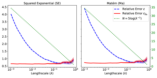
Figure 1: Plots of the average relative errors and 95% confidence intervals achieved by the sample ($\varepsilon$, dashed blue) and thresholded ($\varepsilon_{\widehat{\rho}_{N}}$, solid red) covariance estimators based on sample size ($N$, dotted green) for the squared exponential kernel (left) and Matérn kernel (right) over 100 trials.

To quantify the performance of each of the estimators, we compute their relative errors

$$\varepsilon:=\frac{\|\widehat{\mathcal{C}}-\mathcal{C}\|}{\|\mathcal{C}\|},\qquad\varepsilon_{\widehat{\rho}_{N}}:=\frac{\|\widehat{\mathcal{C}}_{\widehat{\rho}_{N}}-\mathcal{C}\|}{\|\mathcal{C}\|}.$$

The experiment is repeated a total of 100 times for each lengthscale. In Figure 1, we plot average relative errors as well as 95% confidence intervals over the 100 trials for both squared exponential and Matérn models, along with the sample size for each lengthscale setting. Our theoretical results are clearly illustrated: taking only $N\asymp\log(\lambda^{-1})$ samples, the relative error in the thresholded covariance operator remains constant as the lengthscale decreases, whereas the relative error in the sample covariance operator diverges. Notice that Figure 1 also shows that thresholding can increase the relative error for fields with large correlation lengthscale.

2.3 Application in Ensemble Kalman Filters

Nonlinear filtering is concerned with online estimation of the state of a dynamical system from partial and noisy observations. Filtering algorithms blend the dynamics and observations by sequentially solving inverse problems of the form

$$y=\mathcal{A}u+\eta,$$ (2.9)

where $y\in\mathbb{R}^{d_{y}}$ denotes the observation, $u\in L^{2}(D)$ denotes the state, $\mathcal{A}:L^{2}(D)\to\mathbb{R}^{d_{y}}$ is a linear observation operator, and $\eta\sim\mathcal{N}(0,\Gamma)$ is the observation error with positive definite covariance matrix $\Gamma$. In Bayesian filtering [Sanz-Alonso, Stuart and Taeb [2023]], the model dynamics define a prior or forecast distribution on the state, which is combined with the data likelihood implied by the observation model (2.9) to obtain a posterior or analysis distribution.

Ensemble Kalman filters (EnKFs) rely on an ensemble of particles $\{u_{n}\}_{n=1}^{N}$ to represent the forecast distribution [Evensen [2009]]. Taking as input a forecast ensemble $\{u_{n}\}_{n=1}^{N}\stackrel{{\scriptstyle\text{i.i.d.}}}{{\sim}}\mathcal{N}(0,\mathcal{C})$ and observed data $y$ generated according to (2.9), EnKFs produce an analysis ensemble $\{\upsilon_{n}\}_{n=1}^{N}$. Each analysis particle $\upsilon_{n}$ is obtained by nudging a forecast particle $u_{n}$ towards the observed data $y.$ The amount of nudging is controlled by a Kalman gain operator to be estimated using the first two moments of the forecast ensemble. In this subsection we show that thresholded covariance operator estimators within the EnKF analysis step can dramatically reduce the ensemble size required to approximate an idealized mean-field EnKF that uses the population moments of the forecast distribution.

Define the mean-field EnKF analysis update by

$$\upsilon_{n}^{\star} :=u_{n}+\mathscr{K}(\mathcal{C})\bigl{(}y-\mathcal{A}u_{n}-\eta_{n}\bigr{)},\qquad 1\leq n\leq N,$$ (2.10)

where $\{\eta_{n}\}_{n=1}^{N}\stackrel{{\scriptstyle\text{i.i.d.}}}{{\sim}}\mathcal{N}(0,\Gamma)$ and

$$\mathscr{K}(\mathcal{C}):=\mathcal{C}\mathcal{A}^{*}(\mathcal{A}\mathcal{C}\mathcal{A}^{*}+\Gamma)^{-1}$$ (2.11)

denotes the Kalman gain. Practical algorithms do not have access to the forecast distribution, and rely instead on the forecast ensemble to estimate both $\mathcal{C}$ and $\mathscr{K}$. We will investigate two popular analysis steps, given by

$$\upsilon_{n} :=u_{n}+\mathscr{K}(\widehat{\mathcal{C}})\bigl{(}y-\mathcal{A}u_{n}-\eta_{n}\bigr{)},\qquad 1\leq n\leq N,$$ (2.12)

$$\upsilon_{n}^{\,\rho} :=u_{n}+\mathscr{K}(\widehat{\mathcal{C}}_{\rho_{N}})\bigl{(}y-\mathcal{A}u_{n}-\eta_{n}\bigr{)},\ \qquad 1\leq n\leq N.$$ (2.13)

The analysis step in (2.12) is known as the perturbed observation or stochastic EnKF [Burgers, Jan van Leeuwen and Evensen [1998]]. For simplicity of exposition, we will assume here that when updating $u_{n},$ this particle is not included in the sample covariance $\widehat{\mathcal{C}}$ used to define the Kalman gain. This slight modification of the sample covariance will facilitate a cleaner statement and proof of our main result, Theorem 2.7, without altering the qualitative behavior of the algorithm. The analysis step in (2.13) is based on a thresholded covariance operator estimator. Again, we assume that the thresholded estimator $\widehat{\mathcal{C}}_{\rho_{N}}$ is defined without using the particle $u_{n}.$ The following result is a direct consequence of our theory on covariance operator estimation in the small lengthscale regime. The proof can be found in Section 5.

Theorem 2.7 (Approximation of Mean-Field EnKF).

Suppose that Assumptions 2.1 and 2.4 hold. Let $y$ be generated according to (2.9) with bounded observation operator $\mathcal{A}:L^{2}(D)\to\mathbb{R}^{d_{y}}$. Let $\upsilon_{n}^{\star}$ be the mean-field EnKF update in (2.10), and let $\upsilon_{n}$ and $\upsilon_{n}^{\,\rho}$ be the EnKF and localized EnKF updates in (2.12) and (2.13). Let $c_{0}\gtrsim 1$ be an absolute constant and set

$$\rho_{N}\asymp\frac{c_{0}}{\sqrt{N}}\Big{(}\frac{1}{N}\sum_{n=1}^{N}\sup_{x\in D}u_{n}(x)\Big{)}.$$

Then,

$$\mathbb{E}\mathopen{}\mathclose{{}\left[|\upsilon_{n}-\upsilon_{n}^{\star}|\mid u_{n},\eta_{n}}\right] \lesssim c\bigg{[}c(d)\bigg{(}\sqrt{\frac{\lambda^{-d}}{N}}\lor\frac{\lambda^{-d}}{N}\bigg{)}\bigg{]},$$

$$\mathbb{E}\mathopen{}\mathclose{{}\left[|\upsilon_{n}^{\,\rho}-\upsilon_{n}^{\star}|\mid u_{n},\eta_{n}}\right] \lesssim c\bigg{[}c(d,q)\bigg{(}\frac{\log(\lambda^{-d})}{N}\bigg{)}^{\frac{1-q}{2}}\bigg{]},$$

where $c=\|\mathcal{A}\|\|\Gamma^{-1}\|\|\mathcal{C}\||y-\mathcal{A}u_{n}-\eta_{n}|$.

3 Thresholded Estimation of Covariance Operators

This section studies thresholded estimation of covariance operators in the general setting of Assumption 2.1. In Subsection 3.1 we establish concentration bounds for the empirical thresholding parameter $\widehat{\rho}_{N}$ defined in (2.2). In Subsection 3.2 we show uniform error bounds on the sample covariance function estimator $\widehat{k}(x,x^{\prime})$. These results are used in Subsection 3.3 to prove our first main result, Theorem 2.2.

3.1 Concentration of the Empirical Thresholding Parameter

The following auxiliary result can be found in [Van Handel [2014], Lemma 6.15].

Lemma 3.1.

Under Assumption 2.1 (i), it holds with probability at least $1-2e^{-t}$ that

$$\mathopen{}\mathclose{{}\left|\frac{1}{N}\sum_{n=1}^{N}\sup_{x\in D}u_{n}(x)-\mathbb{E}\mathopen{}\mathclose{{}\left[\sup_{x\in D}u(x)}\right]}\right|\leq\sqrt{\frac{2t}{N}}.$$

Proof.

By Gaussian concentration, $\sup_{x\in D}u(x)$ is $\sup_{x\in D}\operatorname{Var}\mathopen{}\mathclose{{}\left[u(x)}\right]$-sub-Gaussian. Since under Assumption 2.1 (i), $\sup_{x\in D}\operatorname{Var}\mathopen{}\mathclose{{}\left[u(x)}\right]=1,$ a Chernoff bound argument gives the result. ∎

The next result establishes moment and concentration bounds for the estimator $\widehat{\rho}_{N}$ of the thresholding parameter $\rho_{N}.$ The proof relies heavily on Lemma 3.1.

Lemma 3.2.

Under the setting of Theorem 2.2, it holds that

1. For any $p\geq 1$, $\mathbb{E}\big{[}\,\widehat{\rho}_{N}^{\,p}\big{]}\lesssim_{p}\rho_{N}^{p}$.

2. For any $t\in(0,1)$,

   $$\mathbb{P}\mathopen{}\mathclose{{}\left[\,\widehat{\rho}_{N}<t\rho_{N}}\right] \leq 2\,e^{-\frac{1}{2}(1-\sqrt{t})^{2}N(\mathbb{E}[\sup_{x\in D}u(x)])^{2}}\mathbf{1}\big{\{}\mathbb{E}[\sup_{x\in D}u(x)]\geq 1/\sqrt{N}\big{\}}$$ (3.1)

   $$\leq 2\,e^{-\frac{1}{2}(1-\sqrt{t})^{2}N(\rho_{N}\land\,\rho_{N}^{2})}.$$ (3.2)

Proof.

We first prove (A). Without loss of generality, we assume $c_{0}=1$ in the definition of $\widehat{\rho}_{N}$ and $\rho_{N}$ in Theorem 2.2. Let $t>0$ and define $\mathcal{E}_{t}$ to be the event on which $\mathopen{}\mathclose{{}\left|\frac{1}{N}\sum_{n=1}^{N}\sup_{x\in D}u_{n}(x)-\mathbb{E}\mathopen{}\mathclose{{}\left[\sup_{x\in D}u(x)}\right]}\right|\leq t$. It holds on $\mathcal{E}_{t}$ that

$$\widehat{\rho}_{N} \leq\frac{1}{N}\lor\frac{\mathbb{E}[\sup_{x\in D}u(x)]+t}{\sqrt{N}}\lor\frac{(\mathbb{E}[\sup_{x\in D}u(x)]+t)^{2}}{N}$$

$$\leq\frac{1}{N}\lor\frac{2\mathbb{E}[\sup_{x\in D}u(x)]}{\sqrt{N}}\lor\frac{2t}{\sqrt{N}}\lor\frac{4(\mathbb{E}[\sup_{x\in D}u(x)])^{2}}{N}\lor\frac{4t^{2}}{N}$$

$$\leq 4\rho_{N}\lor\frac{2t}{\sqrt{N}}\lor\frac{4t^{2}}{N},$$

and $\mathbb{P}(\widehat{\rho}_{N}\leq 4\rho_{N}\lor\frac{2t}{\sqrt{N}}\lor\frac{4t^{2}}{N})\geq\mathbb{P}(\mathcal{E}_{t})\geq 1-2e^{-Nt^{2}/2}$ by Lemma 3.1. It follows then that

$$\mathbb{E}\big{[}\,\widehat{\rho}_{N}^{\,p}\big{]} =p\int_{0}^{\infty}t^{p-1}\,\mathbb{P}\big{[}\,\widehat{\rho}_{N}\geq t\big{]}dt=p\int_{0}^{4\,\rho_{N}}t^{p-1}\,\mathbb{P}\big{[}\,\widehat{\rho}_{N}\geq t\big{]}dt+p\int_{4\,\rho_{N}}^{\infty}t^{p-1}\,\mathbb{P}\big{[}\,\widehat{\rho}_{N}\geq t\big{]}dt$$

$$\leq(4\rho_{N})^{p}+2p\int_{4\,\rho_{N}}^{\infty}t^{p-1}\,e^{-\frac{N}{2}\min\{\frac{Nt^{2}}{4},\frac{Nt}{4}\}}dt\lesssim_{p}\rho_{N}^{p}+\frac{1}{N^{p}}\lesssim_{p}\rho_{N}^{p}.$$

We next show (B). To prove (3.1), we can assume $c_{0}=1$ without loss of generality. Notice that

$$\mathbb{P}[\widehat{\rho}_{N}<t\rho_{N}] =\mathbb{P}\mathopen{}\mathclose{{}\left[\Big{(}\frac{1}{N}<t\rho_{N}\Big{)}\bigcap\Big{(}\frac{1}{\sqrt{N}}\Big{(}\frac{1}{N}\sum_{n=1}^{N}\sup_{x\in D}u_{n}(x)\Big{)}<t\rho_{N}\Big{)}\bigcap\Big{(}\frac{1}{N}\Big{(}\frac{1}{N}\sum_{n=1}^{N}\sup_{x\in D}u_{n}(x)\Big{)}^{2}<t\rho_{N}\Big{)}}\right]$$

$$=1-\mathbb{P}\mathopen{}\mathclose{{}\left[\Big{(}\frac{1}{N}\geq t\rho_{N}\Big{)}\bigcup\Big{(}\frac{1}{\sqrt{N}}\Big{(}\frac{1}{N}\sum_{n=1}^{N}\sup_{x\in D}u_{n}(x)\Big{)}\geq t\rho_{N}\Big{)}\bigcup\Big{(}\frac{1}{N}\Big{(}\frac{1}{N}\sum_{n=1}^{N}\sup_{x\in D}u_{n}(x)\Big{)}^{2}\geq t\rho_{N}\Big{)}}\right].$$

We consider three cases.

Case 1: If $\mathbb{E}[\sup_{x\in D}u(x)]<\frac{1}{\sqrt{N}}$, then $\rho_{N}=\frac{1}{N}$ and $\mathbb{P}[\widehat{\rho}_{N}<t\rho_{N}]\leq 1-\mathbb{P}\Big{[}\frac{1}{N}\geq t\rho_{N}\Big{]}=0$.

Case 2: If $\frac{1}{\sqrt{N}}\leq\mathbb{E}[\sup_{x\in D}u(x)]\leq\sqrt{N}$, then $\rho_{N}=\frac{1}{\sqrt{N}}\mathbb{E}[\sup_{x\in D}u(x)]$ and

$$\mathbb{P}[\widehat{\rho}_{N}<t\rho_{N}] \leq 1-\mathbb{P}\mathopen{}\mathclose{{}\left[\Big{(}\frac{1}{\sqrt{N}}\Big{(}\frac{1}{N}\sum_{n=1}^{N}\sup_{x\in D}u_{n}(x)\Big{)}\geq t\rho_{N}\Big{)}}\right]=1-\mathbb{P}\mathopen{}\mathclose{{}\left[\frac{1}{N}\sum_{n=1}^{N}\sup_{x\in D}u_{n}(x)\geq t\,\mathbb{E}[\sup_{x\in D}u(x)]}\right]$$

$$\leq\mathbb{P}\mathopen{}\mathclose{{}\left[\Big{|}\frac{1}{N}\sum_{n=1}^{N}\sup_{x\in D}u_{n}(x)-\mathbb{E}[\sup_{x\in D}u(x)]\Big{|}\geq(1-t)\mathbb{E}[\sup_{x\in D}u(x)]}\right]$$

$$\leq 2\exp\Big{(}-\frac{1}{2}(1-t)^{2}N(\mathbb{E}[\sup_{x\in D}u(x)])^{2}\Big{)},$$

where the last step follows by Lemma 3.1.

Case 3: If $\mathbb{E}[\sup_{x\in D}u(x)]>\sqrt{N}$, then $\rho_{N}=\frac{1}{N}(\mathbb{E}[\sup_{x\in D}u(x)])^{2}$ and

$$\mathbb{P}[\widehat{\rho}_{N}<t\rho_{N}] \leq 1-\mathbb{P}\mathopen{}\mathclose{{}\left[\frac{1}{N}\Big{(}\frac{1}{N}\sum_{n=1}^{N}\sup_{x\in D}u_{n}(x)\Big{)}^{2}\geq t\rho_{N}}\right]=1-\mathbb{P}\mathopen{}\mathclose{{}\left[\Big{|}\frac{1}{N}\sum_{n=1}^{N}\sup_{x\in D}u_{n}(x)\Big{|}\geq\sqrt{t}\,\mathbb{E}[\sup_{x\in D}u(x)]}\right]$$

$$\leq\mathbb{P}\mathopen{}\mathclose{{}\left[\Big{|}\frac{1}{N}\sum_{n=1}^{N}\sup_{x\in D}u_{n}(x)-\mathbb{E}[\sup_{x\in D}u(x)]\Big{|}\geq(1-\sqrt{t})\mathbb{E}[\sup_{x\in D}u(x)]}\right]$$

$$\leq 2\exp\Big{(}-\frac{1}{2}(1-\sqrt{t})^{2}N(\mathbb{E}[\sup_{x\in D}u(x)])^{2}\Big{)}.$$

Combining the three cases above and noticing that $(1-\sqrt{t})^{2}\leq(1-t)^{2}$ for $t\in(0,1)$ yields the first inequality in (3.1). To prove (3.2), recall that $1\leq c_{0}\leq\sqrt{N}$ in the definition of $\rho_{N}$. If $\mathbb{E}[\sup_{x\in D}u(x)]<1/\sqrt{N}$, then (3.2) is trivial. If $\frac{1}{\sqrt{N}}\leq\mathbb{E}[\sup_{x\in D}u(x)]\leq\sqrt{N}$, then $\rho_{N}=\frac{c_{0}}{\sqrt{N}}\mathbb{E}[\sup_{x\in D}u(x)]$ and $N(\mathbb{E}[\sup_{x\in D}u(x)])^{2}=\frac{N^{2}\rho_{N}^{2}}{c_{0}^{2}}\geq N\rho_{N}^{2}$, so that

$$2\,e^{-\frac{1}{2}(1-\sqrt{t})^{2}N(\mathbb{E}[\sup_{x\in D}u(x)])^{2}}\mathbf{1}\big{\{}\mathbb{E}[\sup_{x\in D}u(x)]\geq 1/\sqrt{N}\big{\}}\leq 2\,e^{-\frac{1}{2}(1-\sqrt{t})^{2}N\rho_{N}^{2}}.$$

If $\mathbb{E}[\sup_{x\in D}u(x)]>\sqrt{N}$, then $\rho_{N}=\frac{c_{0}}{N}(\mathbb{E}[\sup_{x\in D}u(x)])^{2}$ and $N(\mathbb{E}[\sup_{x\in D}u(x)])^{2}=\frac{N^{2}\rho_{N}}{c_{0}}\geq N^{3/2}\rho_{N}\geq N\rho_{N}$, so that

$$2\,e^{-\frac{1}{2}(1-\sqrt{t})^{2}N(\mathbb{E}[\sup_{x\in D}u(x)])^{2}}\mathbf{1}\big{\{}\mathbb{E}[\sup_{x\in D}u(x)]\geq 1/\sqrt{N}\big{\}}\leq 2\,e^{-\frac{1}{2}(1-\sqrt{t})^{2}N\rho_{N}}.\qed$$

3.2 Covariance Function Estimation

In this subsection we establish uniform error bounds on the sample covariance function estimator. These bounds will play a central role in our analysis of thresholded estimation of covariance operators developed in the next subsection. We first establish a high-probability bound, which is uniform over both arguments of the covariance function.

Proposition 3.3.

Under Assumption 2.1, there exist positive absolute constants $c_{1},c_{2}$ such that, for all $t\geq 1$, it holds with probability at least $1-c_{1}e^{-c_{2}t}$ that

$$\sup_{x,x^{\prime}\in D}\mathopen{}\mathclose{{}\left|\widehat{k}(x,x^{\prime})-k(x,x^{\prime})}\right|\lesssim\mathopen{}\mathclose{{}\left[\mathopen{}\mathclose{{}\left(\frac{t}{N}\vee\sqrt{\frac{t}{N}}}\right)\mathbb{E}\Big{[}\sup_{x\in D}u(x)\Big{]}}\right]\vee\frac{\mathopen{}\mathclose{{}\left(\mathbb{E}\mathopen{}\mathclose{{}\left[\sup_{x\in D}u(x)}\right]}\right)^{2}}{N}.$$

Proof.

We will apply the product empirical process bound in [Mendelson [2016], Theorem 1.13]. To that end, define the evaluation functional at $x\in D$ by

$$\ell_{x}:u\longmapsto\ell_{x}(u)=u(x)$$

and write

$$\mathopen{}\mathclose{{}\left|\widehat{k}(x,x^{\prime})-k(x,x^{\prime})}\right|=\mathopen{}\mathclose{{}\left|\frac{1}{N}\sum_{n=1}^{N}u_{n}(x)u_{n}(x^{\prime})-\mathbb{E}\mathopen{}\mathclose{{}\left[u(x)u(x^{\prime})}\right]}\right|=\mathopen{}\mathclose{{}\left|\frac{1}{N}\sum_{n=1}^{N}\ell_{x}(u_{n})\ell_{x^{\prime}}(u_{n})-\mathbb{E}\mathopen{}\mathclose{{}\left[\ell_{x}(u)\ell_{x^{\prime}}(u)}\right]}\right|,$$

so that

$$\sup_{x,x^{\prime}\in D}\mathopen{}\mathclose{{}\left|\widehat{k}(x,x^{\prime})-k(x,x^{\prime})}\right|=\sup_{f,g\in\mathcal{F}}\mathopen{}\mathclose{{}\left|\frac{1}{N}\sum_{n=1}^{N}f(u_{n})g(u_{n})-\mathbb{E}\mathopen{}\mathclose{{}\left[f(u)g(u)}\right]}\right|,$$

where $\mathcal{F}:=\{\ell_{x}\}_{x\in D}$ denotes the family of evaluation functionals. Note that $\{\ell_{x}\}_{x\in D}$ are continuous linear functionals on $C(D),$ the space of continuous functions on $D$ endowed with its usual topology. We can then apply [Mendelson [2016], Theorem 1.13] (see also [Al Ghattas and Sanz-Alonso [2022], Theorem B.11]) which implies that, with probability $1-c_{1}e^{-c_{2}t}$,

$$\sup_{x,x^{\prime}\in D}\mathopen{}\mathclose{{}\left|\widehat{k}(x,x^{\prime})-k(x,x^{\prime})}\right|\lesssim\mathopen{}\mathclose{{}\left[\mathopen{}\mathclose{{}\left(\frac{t}{N}\vee\sqrt{\frac{t}{N}}}\right)\mathopen{}\mathclose{{}\left(\sup_{f\in\mathcal{F}}\|f\|_{\psi_{2}}\gamma_{2}\mathopen{}\mathclose{{}\left(\mathcal{F},\psi_{2}}\right)}\right)}\right]\vee\frac{\gamma_{2}^{2}\mathopen{}\mathclose{{}\left(\mathcal{F},\psi_{2}}\right)}{N},$$ (3.3)

where here and henceforth $\gamma_{2}$ denotes Talagrand’s generic complexity [Talagrand [2022], Definition 2.7.3] and $\psi_{2}$ denotes the Orlicz norm with Orlicz function $\psi(x)=e^{x^{2}}-1,$ see e.g. [Vershynin [2018], Definition 2.5.6]. Since $u$ is Gaussian, the $\psi_{2}$-norm of linear functionals is equivalent to the $L^{2}$-norm. Hence,

$$\sup_{f\in\mathcal{F}}\|f\|_{\psi_{2}}\lesssim\sup_{f\in\mathcal{F}}\|f\|_{L^{2}}=\sup_{f\in\mathcal{F}}\sqrt{\mathbb{E}\mathopen{}\mathclose{{}\left[f^{2}(u)}\right]}=\sup_{x\in D}\sqrt{\mathbb{E}\mathopen{}\mathclose{{}\left[u^{2}(x)}\right]}=\sup_{x\in D}\sqrt{k(x,x)}=1,$$ (3.4)

where we used Assumption 2.1 (i) in the last step. Next, to control the complexity $\gamma_{2}\mathopen{}\mathclose{{}\left(\mathcal{F},\psi_{2}}\right),$ let

$$\mathsf{d}(x,x^{\prime}):=\sqrt{\mathbb{E}\mathopen{}\mathclose{{}\left[(u(x)-u(x^{\prime}))^{2}}\right]}=\|\ell_{x}(\cdot)-\ell_{x^{\prime}}(\cdot)\|_{L^{2}(P)},\quad x,x^{\prime}\in D,$$

where $P$ is the distribution of the random function $u$. Then,

$$\gamma_{2}(\mathcal{F},\psi_{2})\overset{(\text{i})}{\lesssim}\gamma_{2}(\mathcal{F},L^{2})=\gamma_{2}(D,\mathsf{d})\overset{(\text{ii})}{\asymp}\mathbb{E}\mathopen{}\mathclose{{}\left[\sup_{x\in D}u(x)}\right],$$ (3.5)

where (i) follows by the equivalence of $\psi_{2}$ and $L^{2}$ norms for linear functionals and (ii) follows by Talagrand’s majorizing-measure theorem [Talagrand [2022], Theorem 2.10.1]. Combining the inequalities (3.3), (3.4), and (3.5) gives the desired result. ∎

Corollary 3.4.

Under Assumption 2.1, it holds that, for any $p\geq 1$,

$$\mathopen{}\mathclose{{}\left(\mathbb{E}\mathopen{}\mathclose{{}\left[\sup_{x,x^{\prime}\in D}\mathopen{}\mathclose{{}\left|\widehat{k}(x,x^{\prime})-k(x,x^{\prime})}\right|^{p}}\right]}\right)^{\frac{1}{p}}\lesssim_{p}\frac{\mathbb{E}\mathopen{}\mathclose{{}\left[\sup_{x\in D}u(x)}\right]}{\sqrt{N}}\vee\frac{\mathopen{}\mathclose{{}\left(\mathbb{E}\mathopen{}\mathclose{{}\left[\sup_{x\in D}u(x)}\right]}\right)^{2}}{N}.$$

Proof.

The result follows by integrating the tail bound in Proposition 3.3. ∎

In contrast to Proposition 3.3, the following result provides uniform control over the error when holding fixed one of the two covariance function inputs. For this easier estimation task, we obtain an improved exponential tail bound that we will use in the proof of Theorem 2.2.

Proposition 3.5.

Suppose that Assumption 2.1 holds. Let $1\leq c_{0}\leq N$ and set

$$\rho_{N}:=c_{0}\mathopen{}\mathclose{{}\left[\frac{1}{N}\lor\frac{1}{\sqrt{N}}\mathbb{E}\Big{[}\sup_{x\in D}u(x)\Big{]}\lor\frac{1}{N}\Big{(}\mathbb{E}\Big{[}\sup_{x\in D}u(x)\Big{]}\Big{)}^{2}}\right].$$

Then, for every $x^{\prime}\in D$, it holds with probability at least $1-4e^{-c_{1}N(\rho_{N}\land\,\rho_{N}^{2})}$ that

$$\sup_{x\in D}\,\mathopen{}\mathclose{{}\left|\widehat{k}(x,x^{\prime})-k(x,x^{\prime})}\right|\lesssim\rho_{N}.$$

Proof.

We will apply the multiplier empirical process bound in [Mendelson [2016], Theorem 4.4]. To that end, we write

$$\mathopen{}\mathclose{{}\left|\widehat{k}(x,x^{\prime})-k(x,x^{\prime})}\right|=\mathopen{}\mathclose{{}\left|\frac{1}{N}\sum_{n=1}^{N}u_{n}(x)u_{n}(x^{\prime})-\mathbb{E}\mathopen{}\mathclose{{}\left[u(x)u(x^{\prime})}\right]}\right|=\mathopen{}\mathclose{{}\left|\frac{1}{N}\sum_{n=1}^{N}\ell_{x}(u_{n})\ell_{x^{\prime}}(u_{n})-\mathbb{E}\mathopen{}\mathclose{{}\left[\ell_{x}(u)\ell_{x^{\prime}}(u)}\right]}\right|,$$

so that for the class $\mathcal{F}:=\{\ell_{x}\}_{x\in D}$ of evaluation functionals and for a fixed $g\in\mathcal{F}$, we have

$$\sup_{x\in D}\,\mathopen{}\mathclose{{}\left|\widehat{k}(x,x^{\prime})-k(x,x^{\prime})}\right| =\sup_{f\in\mathcal{F}}\,\mathopen{}\mathclose{{}\left|\frac{1}{N}\sum_{n=1}^{N}f(u_{n})g(u_{n})-\mathbb{E}\mathopen{}\mathclose{{}\left[f(u)g(u)}\right]}\right|$$

$$=\frac{1}{N}\sup_{f\in\mathcal{F}}\,\mathopen{}\mathclose{{}\left|\sum_{n=1}^{N}\big{(}f(u_{n})\xi_{n}-\mathbb{E}\mathopen{}\mathclose{{}\left[f(u)\xi}\right]\big{)}}\right|,$$

where $\xi_{n}:=g(u_{n}).$ Note that $\xi_{1},\dots,\xi_{N}$ are i.i.d. copies of $\xi\sim\mathcal{N}\bigl{(}0,k(x^{\prime},x^{\prime})\bigr{)},$ where $x^{\prime}\in D$ is the point indexed by $g$. By [Mendelson [2016], Theorem 4.4] we have that for any $s,t\geq 1,$ it holds with probability at least $1-2e^{-c_{1}s^{2}(\mathbb{E}[\sup_{x\in D}u(x)])^{2}}-2e^{-c_{1}Nt^{2}}$ that

$$\sup_{x\in D}|\widehat{k}(x,x^{\prime})-k(x,x^{\prime})|\lesssim\frac{st\|\xi\|_{\psi_{2}}\,\mathbb{E}[\sup_{x\in D}u(x)]}{\sqrt{N}}\leq\frac{st\,\mathbb{E}[\sup_{x\in D}u(x)]}{\sqrt{N}},$$ (3.6)

where the last inequality follows by the fact that $\|\xi\|_{\psi_{2}}\leq\sqrt{k(x^{\prime},x^{\prime})}\leq\sup_{x\in D}\sqrt{k(x,x)}=1.$ We consider three cases:

Case 1: If $\mathbb{E}[\sup_{x\in D}u(x)]<\frac{1}{\sqrt{N}}$, then $\rho_{N}=\frac{c_{0}}{N}<1$. We take

$$s=\frac{c_{0}}{\sqrt{N}\,\mathbb{E}[\sup_{x\in D}u(x)]}>1,\qquad t=1,$$

and then (3.6) implies that it holds with probability at least $1-2e^{-c_{1}c_{0}^{2}/N}-2e^{-c_{1}N}\overset{\text{(i)}}{\geq}1-4e^{-c_{1}c_{0}^{2}/N}=1-4e^{-c_{1}N\rho_{N}^{2}}$ that

$$\sup_{x\in D}|\widehat{k}(x,x^{\prime})-k(x,x^{\prime})|\lesssim\frac{st\,\mathbb{E}[\sup_{x\in D}u(x)]}{\sqrt{N}}=\frac{c_{0}}{N}=\rho_{N},$$

where (i) follows since $c_{0}<N$ by assumption.

Case 2: If $\frac{1}{\sqrt{N}}\leq\mathbb{E}[\sup_{x\in D}u(x)]\leq\sqrt{N}$, then $\rho_{N}=\frac{c_{0}}{\sqrt{N}}\mathbb{E}[\sup_{x\in D}u(x)]$. In this case, if $\rho_{N}=\frac{c_{0}}{\sqrt{N}}\mathbb{E}[\sup_{x\in D}u(x)]>1$, we take

$$s=\sqrt{\frac{c_{0}\sqrt{N}}{\mathbb{E}[\sup_{x\in D}u(x)]}}\geq 1,\qquad t=\sqrt{\frac{c_{0}}{\sqrt{N}}\mathbb{E}[\sup_{x\in D}u(x)]}>1,$$

and then (3.6) implies that it holds with probability at least $1-4e^{-c_{1}c_{0}\sqrt{N}\mathbb{E}[\sup_{x\in D}u(x)]}=1-4e^{-c_{1}N\rho_{N}}$ that

$$\sup_{x\in D}|\widehat{k}(x,x^{\prime})-k(x,x^{\prime})|\lesssim\frac{st\,\mathbb{E}[\sup_{x\in D}u(x)]}{\sqrt{N}}=\frac{c_{0}}{\sqrt{N}}\mathbb{E}[\sup_{x\in D}u(x)]=\rho_{N}.$$

If $\rho_{N}=\frac{c_{0}}{\sqrt{N}}\mathbb{E}[\sup_{x\in D}u(x)]\leq 1$, then we take $s=c_{0}\geq 1$ and $t=1$, and (3.6) implies that, with probability at least

$$1-2e^{-c_{1}c_{0}^{2}(\mathbb{E}[\sup_{x\in D}u(x)])^{2}}-2e^{-c_{1}N}\geq 1-4e^{-c_{1}c_{0}^{2}(\mathbb{E}[\sup_{x\in D}u(x)])^{2}}=1-4e^{-c_{1}N\rho_{N}^{2}},$$

it holds that

$$\sup_{x\in D}|\widehat{k}(x,x^{\prime})-k(x,x^{\prime})|\lesssim\frac{st\,\mathbb{E}[\sup_{x\in D}u(x)]}{\sqrt{N}}=\frac{c_{0}}{\sqrt{N}}\mathbb{E}[\sup_{x\in D}u(x)]=\rho_{N}.$$

Case 3: If $\mathbb{E}[\sup_{x\in D}u(x)]>\sqrt{N}$, then $\rho_{N}=\frac{c_{0}}{N}(\mathbb{E}[\sup_{x\in D}u(x)])^{2}>1.$ We take

$$s=\sqrt{c_{0}}\geq 1,\qquad t=\sqrt{c_{0}}\frac{\mathbb{E}[\sup_{x\in D}u(x)]}{\sqrt{N}}>1,$$

and (3.6) implies that it holds with probability at least $1-4e^{-c_{1}c_{0}(\mathbb{E}[\sup_{x\in D}u(x)])^{2}}=1-4e^{-c_{1}N\rho_{N}}$ that

$$\sup_{x\in D}|\widehat{k}(x,x^{\prime})-k(x,x^{\prime})|\lesssim\frac{st\,\mathbb{E}[\sup_{x\in D}u(x)]}{\sqrt{N}}=\frac{c_{0}}{N}(\mathbb{E}[\sup_{x\in D}u(x)])^{2}=\rho_{N}.$$

Combining the three cases above gives the desired result. ∎

3.3 Proof of Theorem 2.2

Proof of Theorem 2.2..

The operator norm can be upper bounded as

$$\|\widehat{\mathcal{C}}_{\widehat{\rho}_{N}}-\mathcal{C}\|\leq\sup_{x\in D}\int_{D}\,\big{|}\widehat{k}_{\widehat{\rho}_{N}}(x,x^{\prime})-k(x,x^{\prime})\big{|}\,dx^{\prime}.$$

Let $\Omega_{x}:=\mathopen{}\mathclose{{}\left\{x^{\prime}\in D:|k(x,x^{\prime})|\geq\widehat{\rho}_{N}}\right\}$ and let $\Omega^{c}_{x}$ be its complement. Then, we have

$$\begin{split}&\mathbb{E}\|\widehat{\mathcal{C}}_{\widehat{\rho}_{N}}-\mathcal{C}\|^{p}\leq\mathbb{E}\mathopen{}\mathclose{{}\left[\bigg{(}\sup_{x\in D}\int_{D}\ \big{|}\widehat{k}_{\widehat{\rho}_{N}}(x,x^{\prime})-k(x,x^{\prime})\big{|}\ dx^{\prime}\bigg{)}^{p}}\right]\\ &\leq 2^{p-1}\mathbb{E}\mathopen{}\mathclose{{}\left[\bigg{(}\sup_{x\in D}\int_{\Omega_{x}}\ \big{|}\widehat{k}_{\widehat{\rho}_{N}}(x,x^{\prime})-k(x,x^{\prime})\big{|}\,dx^{\prime}\bigg{)}^{p}}\right]+2^{p-1}\mathbb{E}\mathopen{}\mathclose{{}\left[\bigg{(}\sup_{x\in D}\int_{\Omega^{c}_{x}}\ \big{|}\widehat{k}_{\widehat{\rho}_{N}}(x,x^{\prime})-k(x,x^{\prime})\big{|}\,dx^{\prime}\bigg{)}^{p}}\right]\\ &\lesssim_{p}\mathbb{E}\mathopen{}\mathclose{{}\left[\bigg{(}\sup_{x\in D}\int_{\Omega_{x}}\ \big{|}\widehat{k}_{\widehat{\rho}_{N}}(x,x^{\prime})-k(x,x^{\prime})\big{|}\,dx^{\prime}\bigg{)}^{p}}\right]+\mathbb{E}\mathopen{}\mathclose{{}\left[\bigg{(}\sup_{x\in D}\int_{\Omega^{c}_{x}}\ |k(x,x^{\prime})|\mathbf{1}\big{\{}|\widehat{k}(x,x^{\prime})|<\widehat{\rho}_{N}\big{\}}\,dx^{\prime}\bigg{)}^{p}}\right]\\ &\hskip 8.5359pt+\mathbb{E}\mathopen{}\mathclose{{}\left[\bigg{(}\sup_{x\in D}\int_{\Omega^{c}_{x}}\ |\widehat{k}(x,x^{\prime})-k(x,x^{\prime})|\mathbf{1}\big{\{}|\widehat{k}(x,x^{\prime})|\geq\widehat{\rho}_{N}\big{\}}\mathbf{1}\big{\{}|\widehat{k}(x,x^{\prime})-k(x,x^{\prime})|<4|k(x,x^{\prime})|\big{\}}\,dx^{\prime}\bigg{)}^{p}}\right]\\ &\hskip 8.5359pt+\mathbb{E}\mathopen{}\mathclose{{}\left[\bigg{(}\sup_{x\in D}\int_{\Omega^{c}_{x}}\ |\widehat{k}(x,x^{\prime})-k(x,x^{\prime})|\mathbf{1}\big{\{}|\widehat{k}(x,x^{\prime})|\geq\widehat{\rho}_{N}\big{\}}\mathbf{1}\big{\{}|\widehat{k}(x,x^{\prime})-k(x,x^{\prime})|\geq 4|k(x,x^{\prime})|\big{\}}\,dx^{\prime}\bigg{)}^{p}}\right]\\ &=:I_{1}+I_{2}+I_{3}+I_{4}.\end{split}$$ (3.7)

We next bound the four terms $\{I_{i}\}_{i=1}^{4}$. To ease notation, we define

$$\|\widehat{k}-k\|_{\max}:=\sup_{x,x^{\prime}\in D}\,|\widehat{k}(x,x^{\prime})-k(x,x^{\prime})|.$$

For $I_{1}$, using that

$$\big{|}\widehat{k}_{\widehat{\rho}_{N}}(x,x^{\prime})-k(x,x^{\prime})\big{|}\leq\big{|}\widehat{k}_{\widehat{\rho}_{N}}(x,x^{\prime})-\widehat{k}(x,x^{\prime})\big{|}+\big{|}\widehat{k}(x,x^{\prime})-k(x,x^{\prime})\big{|}\leq\widehat{\rho}_{N}+\|\widehat{k}-k\|_{\max},$$

we have

$$I_{1}=\mathbb{E}\mathopen{}\mathclose{{}\left[\bigg{(}\sup_{x\in D}\int_{\Omega_{x}}\ \big{|}\widehat{k}_{\widehat{\rho}_{N}}(x,x^{\prime})-k(x,x^{\prime})\big{|}\,dx^{\prime}\bigg{)}^{p}}\right]\leq\mathbb{E}\mathopen{}\mathclose{{}\left[\Big{(}\sup_{x\in D}\mathrm{Vol}(\Omega_{x})\Big{)}^{p}\mathopen{}\mathclose{{}\left(\widehat{\rho}_{N}+\|\widehat{k}-k\|_{\max}}\right)^{p}}\right],$$

where $\mathrm{Vol}(\Omega_{x})$ denotes the Lebesgue measure of $\Omega_{x}.$ Notice that

$$R_{q}^{q}\geq\sup_{x\in D}\int_{D}|k(x,x^{\prime})|^{q}dx^{\prime}\geq\sup_{x\in D}\int_{\Omega_{x}}|k(x,x^{\prime})|^{q}dx^{\prime}\geq\sup_{x\in D}\int_{\Omega_{x}}\widehat{\rho}_{N}^{\ q}dx^{\prime}=\widehat{\rho}_{N}^{\ q}\sup_{x\in D}\mathrm{Vol}(\Omega_{x}).$$

Combining this bound with the trivial bound $\sup_{x}\mathrm{Vol}(\Omega_{x})\leq\mathrm{Vol}(D)=1$ gives

$$\sup_{x\in D}\mathrm{Vol}(\Omega_{x})\leq R^{q}_{q}\widehat{\rho}_{N}^{\,-q}\land 1.$$

Therefore, by Cauchy-Schwarz, we have that

$$I_{1} \leq\mathbb{E}\mathopen{}\mathclose{{}\left[\big{(}R^{q}_{q}\widehat{\rho}_{N}^{\,-q}\land 1\big{)}^{p}(\widehat{\rho}_{N}+\|\widehat{k}-k\|_{\max})^{p}}\right]$$

$$\leq\sqrt{\mathbb{E}\Big{[}\big{(}R^{q}_{q}\widehat{\rho}_{N}^{\,-q}\land 1\big{)}^{2p}\Big{]}\ \mathbb{E}\Big{[}\big{(}\widehat{\rho}_{N}+\|\widehat{k}-k\|_{\max}\big{)}^{2p}\Big{]}}.$$ (3.8)

Using Lemma 3.2 and Corollary 3.4 yields that

$$\mathbb{E}\Big{[}\big{(}\widehat{\rho}_{N}+\|\widehat{k}-k\|_{\max}\big{)}^{2p}\Big{]}\lesssim_{p}\mathbb{E}\big{[}\big{(}\widehat{\rho}_{N}\big{)}^{2p}\big{]}+\mathbb{E}\Big{[}\|\widehat{k}-k\|_{\max}^{2p}\Big{]}\lesssim_{p}\rho_{N}^{2p}.$$ (3.9)

On the other hand,

$$\mathbb{E}\Big{[}\big{(}R^{q}_{q}\widehat{\rho}_{N}^{\,-q}\land 1\big{)}^{2p}\Big{]} =R_{q}^{2pq}\,\mathbb{E}\mathopen{}\mathclose{{}\left[\widehat{\rho}_{N}^{\,-2pq}\land R_{q}^{-2pq}}\right]=R_{q}^{2pq}\int_{0}^{\infty}\mathbb{P}\Big{[}\big{(}\widehat{\rho}_{N}^{\,-2pq}\land R_{q}^{-2pq}\big{)}>t\Big{]}dt$$

$$=R_{q}^{2pq}\int_{0}^{R_{q}^{-2pq}}\mathbb{P}\mathopen{}\mathclose{{}\left[\widehat{\rho}_{N}^{\,-2pq}>t}\right]dt=2pqR_{q}^{2pq}\int_{R_{q}}^{\infty}\mathbb{P}\mathopen{}\mathclose{{}\left[\,\widehat{\rho}_{N}<t}\right]\ t^{-2pq-1}dt.$$

If $R_{q}>\rho_{N}$, then

$$\begin{split}\mathbb{E}\Big{[}\big{(}R^{q}_{q}\widehat{\rho}_{N}^{\,-q}\land 1\big{)}^{2p}\Big{]}&\leq 2pqR_{q}^{2pq}\int_{\rho_{N}}^{\infty}t^{-2pq-1}dt=R_{q}^{2pq}\rho_{N}^{-2pq}.\end{split}$$ (3.10)

If $R_{q}<\rho_{N}$, then

$$\mathbb{E}\Big{[}\big{(}R^{q}_{q}\widehat{\rho}_{N}^{\,-q}\land 1\big{)}^{2p}\Big{]}=2pqR_{q}^{2pq}\mathopen{}\mathclose{{}\left(\int_{\rho_{N}}^{\infty}+\int_{R_{q}}^{\rho_{N}}}\right)\mathbb{P}\mathopen{}\mathclose{{}\left[\widehat{\rho}_{N}<t}\right]\ t^{-2pq-1}dt$$

$$\leq 2pqR_{q}^{2pq}\int_{\rho_{N}}^{\infty}t^{-2pq-1}dt+2pqR_{q}^{2pq}\int_{R_{q}}^{\rho_{N}}\mathbb{P}\mathopen{}\mathclose{{}\left[\widehat{\rho}_{N}<t}\right]\ t^{-2pq-1}dt$$

$$=R_{q}^{2pq}\rho_{N}^{-2pq}+2pqR_{q}^{2pq}\rho_{N}^{-2pq}\int_{R_{q}\rho_{N}^{-1}}^{1}\mathbb{P}\mathopen{}\mathclose{{}\left[\widehat{\rho}_{N}<t\rho_{N}}\right]\ t^{-2pq-1}dt$$

$$\overset{\text{(i)}}{\leq}R_{q}^{2pq}\rho_{N}^{-2pq}+2pqR_{q}^{2pq}\rho_{N}^{-2pq}\int_{R_{q}\rho_{N}^{-1}}^{1}2\exp\Big{(}-\frac{1}{2}(1-\sqrt{t})^{2}N(\rho_{N}\land\,\rho_{N}^{2})\Big{)}t^{-2pq-1}dt$$

$$\overset{\text{(ii)}}{=}R_{q}^{2pq}\rho_{N}^{-2pq}\Bigg{[}1+8pq\int_{0}^{\sqrt{N(\rho_{N}\land\,\rho_{N}^{2})}(1-\sqrt{R_{q}\rho_{N}^{-1}})}\frac{\big{(}N(\rho_{N}\land\,\rho_{N}^{2})\big{)}^{2pq}\exp(-\frac{1}{2}t^{2})}{\big{(}\sqrt{N(\rho_{N}\land\,\rho_{N}^{2})}-t\big{)}^{4pq+1}}\ dt\Bigg{]}$$

$$\overset{\text{(iii)}}{\lesssim}R_{q}^{2pq}\rho_{N}^{-2pq}+R_{q}^{2pq}\rho_{N}^{-2pq}\cdot 8pq\bigg{(}\frac{2R_{q}^{-2pq}\rho_{N}^{2pq}}{4pq}e^{-\frac{1}{8}N(\rho_{N}\land\,\rho_{N}^{2})\big{(}1-\sqrt{R_{q}\rho_{N}^{-1}}\big{)}^{2}}+\frac{2^{4pq}}{4pq}\bigg{)}$$

$$\lesssim_{p}R_{q}^{2pq}\rho_{N}^{-2pq}+e^{-\frac{1}{8}N(\rho_{N}\land\,\rho_{N}^{2})\big{(}1-\sqrt{R_{q}\rho_{N}^{-1}}\big{)}^{2}}$$

$$\overset{\text{(iv)}}{\lesssim}_{p}R_{q}^{2pq}\rho_{N}^{-2pq}+e^{-cN(\rho_{N}\land\,\rho_{N}^{2})},$$ (3.11)

where (i) follows from Lemma 3.2, (ii) follows by a change of variable, and (iii) follows by applying Lemma 3.6 below with $\alpha=\sqrt{N(\rho_{N}\land\,\rho_{N}^{2})}$ and $\beta=\sqrt{N(\rho_{N}\land\,\rho_{N}^{2})}\sqrt{R_{q}\rho_{N}^{-1}}$. To prove (iv), notice that if $R_{q}\leq\frac{1}{4}\rho_{N}$, then $\big{|}1-\sqrt{R_{q}\rho_{N}^{-1}}\big{|}>\frac{1}{2}$ and (iv) holds; if $\frac{1}{4}\rho_{N}<R_{q}<\rho_{N}$, then

$$e^{-\frac{1}{8}N(\rho_{N}\land\,\rho_{N}^{2})\big{(}1-\sqrt{R_{q}\rho_{N}^{-1}}\big{)}^{2}}\leq 1<16^{p}R_{q}^{2p}\rho_{N}^{-2p}\leq 16^{p}R_{q}^{2pq}\rho_{N}^{-2pq}.$$

Combining the inequalities (3.3), (3.9), (3.10), and (3.3) gives that

$$I_{1}\leq\sqrt{\mathbb{E}\Big{[}\big{(}R^{q}_{q}\widehat{\rho}_{N}^{\,-q}\land 1\big{)}^{2p}\Big{]}\ \mathbb{E}\Big{[}\big{(}\widehat{\rho}_{N}+\|\widehat{k}-k\|_{\max}\big{)}^{2p}\Big{]}}\lesssim_{p}R_{q}^{pq}\rho_{N}^{p(1-q)}+\rho_{N}^{p}e^{-cN(\rho_{N}\land\,\rho_{N}^{2})}.$$

For $I_{2}$ and $I_{3}$,

$$\begin{split}I_{2}+I_{3}&=\mathbb{E}\mathopen{}\mathclose{{}\left[\bigg{(}\sup_{x\in D}\int_{\Omega^{c}_{x}}\ \mathopen{}\mathclose{{}\left|k(x,x^{\prime})}\right|\,\mathbf{1}\big{\{}|\widehat{k}(x,x^{\prime})|<\widehat{\rho}_{N}\big{\}}\,dx^{\prime}\bigg{)}^{p}}\right]\\ &\ +\mathbb{E}\mathopen{}\mathclose{{}\left[\bigg{(}\sup_{x\in D}\int_{\Omega^{c}_{x}}\ |\widehat{k}(x,x^{\prime})-k(x,x^{\prime})|\,\mathbf{1}\big{\{}|\widehat{k}(x,x^{\prime})|\geq\widehat{\rho}_{N}\big{\}}\,\mathbf{1}\big{\{}|\widehat{k}(x,x^{\prime})-k(x,x^{\prime})|<4|k(x,x^{\prime})|\big{\}}\,dx^{\prime}\bigg{)}^{p}}\right]\\ &\lesssim\mathbb{E}\mathopen{}\mathclose{{}\left[\bigg{(}\sup_{x\in D}\int_{\Omega^{c}_{x}}\ \mathopen{}\mathclose{{}\left|k(x,x^{\prime})}\right|\,dx^{\prime}\bigg{)}^{p}}\right]=\mathbb{E}\mathopen{}\mathclose{{}\left[\bigg{(}\widehat{\rho}_{N}\sup_{x\in D}\int_{\Omega^{c}_{x}}\mathopen{}\mathclose{{}\left(\frac{|k(x,x^{\prime})|}{\widehat{\rho}_{N}}}\right)\,dx^{\prime}\bigg{)}^{p}}\right]\\ &\overset{\text{(i)}}{\leq}\mathbb{E}\mathopen{}\mathclose{{}\left[\bigg{(}\widehat{\rho}_{N}\sup_{x\in D}\int_{\Omega^{c}_{x}}\mathopen{}\mathclose{{}\left(\frac{|k(x,x^{\prime})|}{\widehat{\rho}_{N}}}\right)^{q}dx^{\prime}\bigg{)}^{p}}\right]\leq\mathbb{E}\mathopen{}\mathclose{{}\left[R_{q}^{pq}\widehat{\rho}_{N}^{\,p(1-q)}}\right]\overset{\text{(ii)}}{\lesssim}_{p}R_{q}^{pq}\rho_{N}^{p(1-q)},\end{split}$$

where (i) follows since $q\in(0,1)$ and $|k(x,x^{\prime})|<\widehat{\rho}_{N}$ for $x^{\prime}\in\Omega_{x}^{c}$. To prove (ii), we notice that if $p(1-q)\leq 1$, then using Jensen’s inequality and Lemma 3.2 yields that $\mathbb{E}[\,\widehat{\rho}_{N}^{\,p(1-q)}]\leq(\mathbb{E}[\,\widehat{\rho}_{N}])^{p(1-q)}\lesssim_{p}\rho_{N}^{p(1-q)}$. If $p(1-q)>1$, Lemma 3.2 implies that $\mathbb{E}[\,\widehat{\rho}_{N}^{\,p(1-q)}]\lesssim_{p}\rho_{N}^{\,p(1-q)}$.

For $I_{4}$,

$$I_{4} =\mathbb{E}\mathopen{}\mathclose{{}\left[\bigg{(}\sup_{x\in D}\int_{\Omega^{c}_{x}}\ |\widehat{k}(x,x^{\prime})-k(x,x^{\prime})|\mathbf{1}\big{\{}|\widehat{k}(x,x^{\prime})|\geq\widehat{\rho}_{N}\big{\}}\mathbf{1}\big{\{}|\widehat{k}(x,x^{\prime})-k(x,x^{\prime})|\geq 4|k(x,x^{\prime})|\big{\}}\,dx^{\prime}\bigg{)}^{p}}\right]$$

$$\overset{\text{(i)}}{\leq}\mathbb{E}\mathopen{}\mathclose{{}\left[\bigg{(}\sup_{x\in D}\int_{\Omega^{c}_{x}}\ |\widehat{k}(x,x^{\prime})-k(x,x^{\prime})|\mathbf{1}\big{\{}|\widehat{k}(x,x^{\prime})|\geq\widehat{\rho}_{N}\big{\}}\mathbf{1}\big{\{}|\widehat{k}(x,x^{\prime})-k(x,x^{\prime})|\geq\frac{2}{3}\widehat{\rho}_{N}\big{\}}\,dx^{\prime}\bigg{)}^{p}}\right]$$

$$\leq\mathbb{E}\mathopen{}\mathclose{{}\left[\bigg{(}\sup_{x\in D}\int_{D}\sup_{x\in D}\,|\widehat{k}(x,x^{\prime})-k(x,x^{\prime})|\,\mathbf{1}\big{\{}\sup_{x\in D}|\widehat{k}(x,x^{\prime})-k(x,x^{\prime})|\geq\frac{2}{3}\widehat{\rho}_{N}\big{\}}\,dx^{\prime}\bigg{)}^{p}}\right]$$

$$=\mathbb{E}\mathopen{}\mathclose{{}\left[\bigg{(}\int_{D}\sup_{x\in D}|\widehat{k}(x,x^{\prime})-k(x,x^{\prime})|\,\mathbf{1}\big{\{}\sup_{x\in D}|\widehat{k}(x,x^{\prime})-k(x,x^{\prime})|\geq\frac{2}{3}\widehat{\rho}_{N}\big{\}}\,dx^{\prime}\bigg{)}^{p}}\right]$$

$$\leq\mathbb{E}\mathopen{}\mathclose{{}\left[\bigg{(}\|\widehat{k}-k\|_{\max}\int_{D}\mathbf{1}\big{\{}\sup_{x\in D}|\widehat{k}(x,x^{\prime})-k(x,x^{\prime})|\geq\frac{2}{3}\widehat{\rho}_{N}\big{\}}\,dx^{\prime}\bigg{)}^{p}}\right]$$

$$\leq\Big{(}\mathbb{E}\big{[}\|\widehat{k}-k\|_{\max}^{2p}\big{]}\Big{)}^{1/2}\mathopen{}\mathclose{{}\left(\mathbb{E}\bigg{[}\Big{(}\int_{D}\mathbf{1}\big{\{}\sup_{x\in D}|\widehat{k}(x,x^{\prime})-k(x,x^{\prime})|\geq\frac{2}{3}\widehat{\rho}_{N}\big{\}}\,dx^{\prime}\Big{)}^{2p}\bigg{]}}\right)^{1/2}$$

$$\overset{\text{(ii)}}{\leq}\Big{(}\mathbb{E}\big{[}\|\widehat{k}-k\|_{\max}^{2p}\big{]}\Big{)}^{1/2}\mathopen{}\mathclose{{}\left(\mathbb{E}\Big{[}\int_{D}\mathbf{1}\big{\{}\sup_{x\in D}|\widehat{k}(x,x^{\prime})-k(x,x^{\prime})|\geq\frac{2}{3}\widehat{\rho}_{N}\big{\}}\,dx^{\prime}\Big{]}}\right)^{1/2}$$

$$=\Big{(}\mathbb{E}\big{[}\|\widehat{k}-k\|_{\max}^{2p}\big{]}\Big{)}^{1/2}\mathopen{}\mathclose{{}\left(\int_{D}\mathbb{P}\mathopen{}\mathclose{{}\left[\sup_{x\in D}|\widehat{k}(x,x^{\prime})-k(x,x^{\prime})|\geq\frac{2}{3}\widehat{\rho}_{N}}\right]dx^{\prime}}\right)^{1/2},$$

where (i) follows since $|\widehat{k}(x,x^{\prime})-k(x,x^{\prime})|\geq 4|k(x,x^{\prime})|$ implies that $|\widehat{k}(x,x^{\prime})|\geq 3|k(x,x^{\prime})|,$ and therefore if $|\widehat{k}(x,x^{\prime})-k(x,x^{\prime})|\geq 4|k(x,x^{\prime})|$ and $|\widehat{k}(x,x^{\prime})|\geq\widehat{\rho}_{N},$ then it holds that

$$|\widehat{k}(x,x^{\prime})-k(x,x^{\prime})|\geq|\widehat{k}(x,x^{\prime})|-|k(x,x^{\prime})|\geq\frac{2}{3}|\widehat{k}(x,x^{\prime})|\geq\frac{2}{3}\widehat{\rho}_{N}.$$

To prove (ii), note that $p\geq 1$ and $\int_{D}\mathbf{1}\mathopen{}\mathclose{{}\left\{\sup_{x\in D}|\widehat{k}(x,x^{\prime})-k(x,x^{\prime})|\geq\frac{2}{3}\widehat{\rho}_{N}}\right\}\,dx^{\prime}\leq 1.$ Next, notice that

$$\mathbb{P}\mathopen{}\mathclose{{}\left[\sup_{x\in D}|\widehat{k}(x,x^{\prime})-k(x,x^{\prime})|\geq\frac{2}{3}\widehat{\rho}_{N}}\right] =\mathbb{P}\mathopen{}\mathclose{{}\left[\frac{2}{3}(\,\rho_{N}-\widehat{\rho}_{N})+\sup_{x\in D}|\widehat{k}(x,x^{\prime})-k(x,x^{\prime})|\geq\frac{2}{3}\rho_{N}}\right]$$

$$\leq\mathbb{P}\mathopen{}\mathclose{{}\left[\sup_{x\in D}|\widehat{k}(x,x^{\prime})-k(x,x^{\prime})|\geq\frac{1}{3}\rho_{N}}\right]+\mathbb{P}\Big{[}\rho_{N}-\widehat{\rho}_{N}\geq\frac{1}{2}\rho_{N}\Big{]}.$$

Lemma 3.2 then implies that

$$\mathbb{P}\Big{[}\rho_{N}-\widehat{\rho}_{N}\geq\frac{1}{2}\rho_{N}\Big{]}=\mathbb{P}\Big{[}\widehat{\rho}_{N}\leq\frac{1}{2}\rho_{N}\Big{]}\lesssim e^{-c_{1}N(\rho_{N}\land\,\rho_{N}^{2})},$$

and Proposition 3.5 gives that

$$\mathbb{P}\mathopen{}\mathclose{{}\left[\sup_{x\in D}|\widehat{k}(x,x^{\prime})-k(x,x^{\prime})|\geq\frac{1}{3}\rho_{N}}\right]\lesssim e^{-c_{2}N(\rho_{N}\land\,\rho_{N}^{2})}.$$

Moreover, Corollary 3.4 yields that $\Big{(}\mathbb{E}\big{[}\|\widehat{k}-k\|_{\max}^{2p}\big{]}\Big{)}^{1/2}\lesssim_{p}\rho_{N}^{p}$. Therefore,

$$I_{4} \leq\Big{(}\mathbb{E}\big{[}\|\widehat{k}-k\|_{\max}^{2p}\big{]}\Big{)}^{1/2}\mathopen{}\mathclose{{}\left(\int_{D}\mathbb{P}\mathopen{}\mathclose{{}\left[\sup_{x\in D}|\widehat{k}(x,x^{\prime})-k(x,x^{\prime})|\geq\frac{2}{3}\widehat{\rho}_{N}}\right]dx^{\prime}}\right)^{1/2}\lesssim_{p}\rho_{N}^{p}e^{-cN(\rho_{N}\land\,\rho_{N}^{2})}.$$

Combining (3.7) with the estimates of $I_{1},I_{2},I_{3}$, and $I_{4}$ gives that

$$\mathbb{E}\|\widehat{\mathcal{C}}_{\widehat{\rho}_{N}}-\mathcal{C}\|^{p}\lesssim_{p}I_{1}+I_{2}+I_{3}+I_{4}\lesssim_{p}R_{q}^{pq}\rho_{N}^{p(1-q)}+\rho_{N}^{p}e^{-cN(\rho_{N}\land\,\rho_{N}^{2})},$$

and hence

$$\big{[}\mathbb{E}\|\widehat{\mathcal{C}}_{\widehat{\rho}_{N}}-\mathcal{C}\|^{p}\big{]}^{\frac{1}{p}}\lesssim_{p}R_{q}^{q}\rho_{N}^{1-q}+\rho_{N}e^{-\frac{c}{p}N(\rho_{N}\land\,\rho_{N}^{2})}.\qed$$

The following lemma was used in the proof of Theorem 2.2.

Lemma 3.6.

For any $\alpha>\beta>0$ and $q>0$, it holds that

$$\int_{0}^{\alpha-\beta}e^{-\frac{1}{2}t^{2}}(\alpha-t)^{-q-1}\,dt\leq\frac{2\beta^{-q}}{q}e^{-\frac{(\alpha-\beta)^{2}}{8}}+\frac{1}{q}\Big{(}\frac{\alpha}{2}\Big{)}^{-q}.$$

Proof.

Integrating by parts gives that

$$\int_{0}^{\alpha-\beta}e^{-\frac{1}{2}t^{2}}(\alpha-t)^{-q-1}dt =\frac{\beta^{-q}}{q}e^{-\frac{(\alpha-\beta)^{2}}{2}}-\frac{\alpha^{-q}}{q}+\int_{0}^{\alpha-\beta}e^{-\frac{1}{2}t^{2}}t\frac{(\alpha-t)^{-q}}{q}dt$$

$$=\frac{\beta^{-q}}{q}e^{-\frac{(\alpha-\beta)^{2}}{2}}-\frac{\alpha^{-q}}{q}+\mathopen{}\mathclose{{}\left(\int_{0}^{\frac{\alpha-\beta}{2}}+\int_{\frac{\alpha-\beta}{2}}^{\alpha-\beta}}\right)e^{-\frac{1}{2}t^{2}}t\frac{(\alpha-t)^{-q}}{q}dt.$$

First,

$$\int_{0}^{\frac{\alpha-\beta}{2}}e^{-\frac{1}{2}t^{2}}t\frac{(\alpha-t)^{-q}}{q}dt\leq\frac{1}{q}\Big{(}\alpha-\frac{\alpha-\beta}{2}\Big{)}^{-q}\int_{0}^{\frac{\alpha-\beta}{2}}e^{-\frac{1}{2}t^{2}}t\,dt\leq\frac{1}{q}\Big{(}\frac{\alpha+\beta}{2}\Big{)}^{-q}\leq\frac{1}{q}\Big{(}\frac{\alpha}{2}\Big{)}^{-q}.$$

Second,

$$\int_{\frac{\alpha-\beta}{2}}^{\alpha-\beta}e^{-\frac{1}{2}t^{2}}t\frac{(\alpha-t)^{-q}}{q}dt\leq\frac{1}{q}(\alpha-(\alpha-\beta))^{-q}\int_{\frac{\alpha-\beta}{2}}^{\alpha-\beta}e^{-\frac{1}{2}t^{2}}t\,dt\leq\frac{\beta^{-q}}{q}e^{-\frac{(\alpha-\beta)^{2}}{8}}.$$

Thus,

$$\int_{0}^{\alpha-\beta}e^{-\frac{1}{2}t^{2}}(\alpha-t)^{-q-1}dt \leq\frac{\beta^{-q}}{q}e^{-\frac{(\alpha-\beta)^{2}}{2}}-\frac{\alpha^{-q}}{q}+\frac{\beta^{-q}}{q}e^{-\frac{(\alpha-\beta)^{2}}{8}}+\frac{1}{q}\Big{(}\frac{\alpha}{2}\Big{)}^{-q}$$

$$\leq\frac{2\beta^{-q}}{q}e^{-\frac{(\alpha-\beta)^{2}}{8}}+\frac{1}{q}\Big{(}\frac{\alpha}{2}\Big{)}^{-q}.\qed$$

4 Small Lengthscale Regime

This section studies thresholded estimation of covariance operators under the small lengthscale regime formalized in Assumption 2.4. We first present three lemmas which establish the sharp scaling of the $L^{q}$-sparsity level, the operator norm of the covariance operator, and the suprema of Gaussian fields in the small lengthscale regime. Combining these lemmas and Theorem 2.2, we then prove Theorem 2.5.

The following result establishes the scaling of the $L^{q}$-sparsity level in the small lengthscale regime.

Lemma 4.1.

Under Assumption 2.4, it holds that

$$\sup_{x\in D}\int_{D}|k(x,x^{\prime})|^{q}dx^{\prime}\asymp\lambda^{d}A(d)\int_{0}^{\infty}k_{1}(r)^{q}r^{d-1}dr,\quad\lambda\to 0.$$

where $A(d)$ denotes the surface area of the unit sphere in $\mathbb{R}^{d}$.

Proof.

Using $k_{\lambda}(r)=k_{1}(\lambda^{-1}r)$, we have that

$$\sup_{x\in D}\int_{D} |k(x,x^{\prime})|^{q}dx^{\prime}\geq\int_{D\times D}k(x,x^{\prime})^{q}dxdx^{\prime}=\int_{[0,1]^{d}\times[0,1]^{d}}k_{\lambda}(|x-x^{\prime}|)^{q}\,dxdx^{\prime}$$

$$=\int_{[0,1]^{d}\times[0,1]^{d}}k_{1}(\lambda^{-1}|x-x^{\prime}|)^{q}\,dxdx^{\prime}=\lambda^{2d}\int_{[0,\lambda^{-1}]^{d}\times[0,\lambda^{-1}]^{d}}k_{1}(|x-x^{\prime}|)^{q}\,dxdx^{\prime}$$

$$\overset{(\text{i})}{=}\lambda^{2d}\int_{[-\lambda^{-1},\lambda^{-1}]^{d}}k_{1}(|w|)^{q}\prod_{j=1}^{d}(\lambda^{-1}-|w_{j}|)\,dw$$

$$=\lambda^{d}\int_{[-\lambda^{-1},\lambda^{-1}]^{d}}k_{1}(|w|)^{q}\prod_{j=1}^{d}(1-\lambda|w_{j}|)\,dw$$

$$\overset{(\text{ii})}{\asymp}\lambda^{d}\int_{\mathbb{R}^{d}}k_{1}(|w|)^{q}\,dw\overset{(\text{iii})}{=}\lambda^{d}A(d)\int_{0}^{\infty}k_{1}(r)^{q}r^{d-1}\,dr,\quad\lambda\to 0,$$ (4.1)

where (i) follows by a change of variables $w=x-x^{\prime},z=x+x^{\prime}$ and integrating $z$, (ii) follows by dominated convergence as $\lambda\to 0$, and (iii) follows from the polar coordinate transform in $\mathbb{R}^{d}$. On the other hand,

$$\begin{split}\sup_{x\in D}\int_{D}|k(x,x^{\prime})|^{q}dx^{\prime}&\leq\sup_{x\in D}\int_{\mathbb{R}^{d}}k(|x-x^{\prime}|)^{q}dx^{\prime}\\ &=\int_{\mathbb{R}^{d}}k(|x^{\prime}|)^{q}\,dx^{\prime}=\lambda^{d}\int_{\mathbb{R}^{d}}k_{1}(|x^{\prime}|)^{q}\,dx^{\prime}=\lambda^{d}A(d)\int_{0}^{\infty}k_{1}(r)^{q}r^{d-1}\,dr,\end{split}$$

which concludes the proof. ∎

Next, we establish the scaling of the operator norm of the covariance operator.

Lemma 4.2.

Under Assumption 2.4, it holds that

$$\|\mathcal{C}\|\asymp\lambda^{d}A(d)\int_{0}^{\infty}k_{1}(r)r^{d-1}dr,\quad\lambda\to 0.$$

where $A(d)$ denotes the surface area of the unit sphere in $\mathbb{R}^{d}$.

Proof.

First, the operator norm can be upper bounded by

$$\|\mathcal{C}\|\leq\sup_{x\in D}\int_{D}|k(x,x^{\prime})|dx^{\prime}\asymp\lambda^{d}A(d)\int_{0}^{\infty}k_{1}(r)r^{d-1}dr,\quad\lambda\to 0,$$

where the last step follows by Lemma 4.1.

For the lower bound, taking the test function $\psi(x)\equiv 1$ yields that

$$\|\mathcal{C}\| =\sup_{\|\psi\|_{L^{2}}=1}\Big{(}\int_{D}\Big{(}\int_{D}k(x,x^{\prime})\psi(x^{\prime})dx^{\prime}\Big{)}^{2}dx\Big{)}^{1/2}\geq\Big{(}\int_{D}\Big{(}\int_{D}k(x,x^{\prime})dx^{\prime}\Big{)}^{2}dx\Big{)}^{1/2}$$

$$\overset{\text{(i)}}{\geq}\frac{1}{\sqrt{\mathrm{Vol}(D)}}\int_{D\times D}k(x,x^{\prime})dxdx^{\prime}\overset{\text{(ii)}}{=}\int_{D\times D}k(x,x^{\prime})dxdx^{\prime}$$

$$\overset{\text{(iii)}}{\asymp}\lambda^{d}A(d)\int_{0}^{\infty}k_{1}(r)r^{d-1}\,dr,\quad\lambda\to 0,$$

where (i) follows by Cauchy-Schwarz inequality, (ii) follows since $\mathrm{Vol}(D)=1$ for $D=[0,1]^{d}$, and (iii) follows from (4) with $q=1$. This completes the proof. ∎

Finally, we establish the scaling of the suprema of Gaussian fields in the small lengthscale regime.

Lemma 4.3.

Under Assumption 2.4 (i), it holds that

$$\mathbb{E}\mathopen{}\mathclose{{}\left[\,\sup_{x\in D}u(x)}\right]\asymp\sqrt{d}\int_{0}^{\infty}\sqrt{k(0)-k(c\sqrt{d}e^{-t^{2}})}\ dt,$$

where $c$ is an absolute constant. Furthermore, if Assumption 2.4 (ii) also holds, then

$$\mathbb{E}\mathopen{}\mathclose{{}\left[\,\sup_{x\in D}u(x)}\right]\asymp\sqrt{k(0)d\log\Big{(}\frac{\sqrt{d}}{s\lambda}\Big{)}}\,\,,\quad\lambda\to 0,$$

where $s>0$ is the unique solution of $k_{1}(s)=\frac{1}{2}k(0),$ which is independent of $\lambda$.

Proof.

By Fernique’s theorem [Fernique et al. [1975]] and the discussion in [Van Handel [2014], Theorem 6.19], for the stationary Gaussian random field $u,$ it holds that

$$\mathbb{E}\mathopen{}\mathclose{{}\left[\,\sup_{x\in D}u(x)}\right]\asymp\int_{0}^{\infty}\sqrt{\log\mathcal{M}(D,\mathsf{d},\varepsilon)}\ d\varepsilon,$$ (4.2)

where $\mathcal{M}(D,\mathsf{d},\varepsilon)$ denotes the smallest cardinality of an $\varepsilon$-net of $D$ in the canonical metric $\mathsf{d}$ given by

$$\mathsf{d}(x,x^{\prime}):=\big{(}\mathbb{E}[(u(x)-u(x^{\prime}))^{2}]\big{)}^{1/2}=\sqrt{2k(0)-2k(|x-x^{\prime}|)}<\sqrt{2k(0)},\quad x,x^{\prime}\in D.$$

This bound implies that $\mathcal{M}(D,\mathsf{d},\varepsilon)=1$ for $\varepsilon\geq\sqrt{2k(0)},$ and hence we can assume without loss of generality that $\varepsilon<\sqrt{2k(0)}$ in the rest of the proof. Next, notice that

$$\mathsf{d}(x,x^{\prime})=\sqrt{2k(0)-2k(|x-x^{\prime}|)}\leq\varepsilon\quad\Longleftrightarrow\quad|x-x^{\prime}|\leq k^{-1}(k(0)-\varepsilon^{2}/2),$$

where $k^{-1}$ is the inverse function of $k$. By the standard volume argument [Vershynin [2018], Proposition 4.2.12],

$$\begin{split}\mathcal{M}(D,\mathsf{d},\varepsilon)&=\mathcal{M}\bigl{(}D,|\cdot|,k^{-1}(k(0)-\varepsilon^{2}/2)\bigr{)}\\ &\geq\mathopen{}\mathclose{{}\left(\frac{1}{k^{-1}(k(0)-\varepsilon^{2}/2)}}\right)^{d}\frac{\mathrm{Vol}(D)}{\mathrm{Vol}(B_{2}^{d})}\geq\frac{1}{c_{1}}\mathopen{}\mathclose{{}\left(\frac{1}{k^{-1}(k(0)-\varepsilon^{2}/2)}}\right)^{d}\mathopen{}\mathclose{{}\left(\frac{d}{2\pi e}}\right)^{d/2},\end{split}$$

where we used that $\mathrm{Vol}(D)=1$ and that, for the Euclidean unit ball $B_{2}^{d},$ it holds that $\mathrm{Vol}(B_{2}^{d})\leq c_{1}(2\pi e/d)^{d/2}$ for some absolute constant $c_{1}>1$. On the other hand, using the fact that $D=[0,1]^{d}\subset\sqrt{d}B_{2}^{d}$, as well as $\mathcal{M}(B_{2}^{d},|\cdot|,\varepsilon)\leq(3/\varepsilon)^{d}$ for $\varepsilon\leq 1$ [Vershynin [2018], Corollary 4.2.13],

$$\begin{split}&\mathcal{M}(D,\mathsf{d},\varepsilon)=\mathcal{M}\bigl{(}D,|\cdot|,k^{-1}(k(0)-\varepsilon^{2}/2)\bigr{)}\\ &\leq\mathcal{M}\bigl{(}B_{2}^{d},|\cdot|,d^{-1/2}k^{-1}(k(0)-\varepsilon^{2}/2)\bigr{)}\leq\mathopen{}\mathclose{{}\left[\mathopen{}\mathclose{{}\left(\frac{3}{k^{-1}(k(0)-\varepsilon^{2}/2)}}\right)^{d}d^{\,d/2}}\right]\lor 1,\quad\varepsilon<\sqrt{2k(0)}.\end{split}$$

Therefore, (4.2) and the bounds we just established on the covering number $\mathcal{M}(D,\mathsf{d},\varepsilon)$ imply that

$$\begin{split}\mathbb{E}\mathopen{}\mathclose{{}\left[\,\sup_{x\in D}u(x)}\right]&\asymp\int_{0}^{\sqrt{2k(0)}}\sqrt{\log\mathopen{}\mathclose{{}\left(\frac{1}{c_{1}}\mathopen{}\mathclose{{}\left(\frac{1}{k^{-1}(k(0)-\varepsilon^{2}/2)}}\right)^{d}\mathopen{}\mathclose{{}\left(\frac{d}{2\pi e}}\right)^{d/2}}\right)\vee 0}\ d\varepsilon\\ &\asymp\sqrt{d}\int_{0}^{\sqrt{2k(0)}}\sqrt{\log\mathopen{}\mathclose{{}\left(\frac{c\sqrt{d}}{k^{-1}(k(0)-\varepsilon^{2}/2)}}\right)\vee 0}\ d\varepsilon.\end{split}$$

By a change of variable $t:=\sqrt{\log\mathopen{}\mathclose{{}\left(\frac{c\sqrt{d}}{k^{-1}(k(0)-\varepsilon^{2}/2)}}\right)}$, then $\varepsilon=\sqrt{2\mathopen{}\mathclose{{}\left(k(0)-k(c\sqrt{d}e^{-t^{2}})}\right)}$ and

$$\begin{split}\mathbb{E}\mathopen{}\mathclose{{}\left[\,\sup_{x\in D}u(x)}\right]&\asymp\sqrt{d}\int_{0}^{\infty}-t\,\frac{d}{dt}\mathopen{}\mathclose{{}\left(\sqrt{k(0)-k(c\sqrt{d}e^{-t^{2}})}}\right)\ dt\\ &=\sqrt{d}\mathopen{}\mathclose{{}\left(-t\sqrt{k(0)-k(c\sqrt{d}e^{-t^{2}})}\,\Big{|}_{0}^{\infty}+\int_{0}^{\infty}\sqrt{k(0)-k(c\sqrt{d}e^{-t^{2}})}\ dt}\right)\\ &=\sqrt{d}\int_{0}^{\infty}\sqrt{k(0)-k(c\sqrt{d}e^{-t^{2}})}\ dt,\end{split}$$

where in the last equality we used that $k(0)-k(c\sqrt{d}e^{-t^{2}})\asymp c\sqrt{d}e^{-t^{2}}$ as $t\to\infty$ since $k(r)$ is assumed to be differentiable at $r=0$.

Furthermore, if Assumption 2.4 (ii) also holds, let $s>0$ be the unique solution of $k_{1}(s)=\frac{1}{2}k(0),$ which is independent of $\lambda$. Then, for $\lambda<c\sqrt{d}/s$,

$$\begin{split}\mathbb{E}\mathopen{}\mathclose{{}\left[\,\sup_{x\in D}u(x)}\right]&\asymp\sqrt{d}\int_{0}^{\infty}\sqrt{k(0)-k_{\lambda}(c\sqrt{d}e^{-t^{2}})}\ dt=\sqrt{d}\int_{0}^{\infty}\sqrt{k(0)-k_{1}(c\lambda^{-1}\sqrt{d}e^{-t^{2}})}\ dt\\ &=\sqrt{d}\mathopen{}\mathclose{{}\left[\int_{t<\sqrt{\log\big{(}\frac{c\sqrt{d}}{s\lambda}\big{)}}}+\int_{t>\sqrt{\log\big{(}\frac{c\sqrt{d}}{s\lambda}\big{)}}}}\right]\sqrt{k(0)-k_{1}(c\lambda^{-1}\sqrt{d}e^{-t^{2}})}\ dt=:I_{1}+I_{2}.\end{split}$$

For the first term $I_{1}$, we have

$$\sqrt{\frac{k(0)d}{2}}\sqrt{\log\Big{(}\frac{c\sqrt{d}}{s\lambda}\Big{)}}\leq I_{1}\leq\sqrt{k(0)d}\sqrt{\log\Big{(}\frac{c\sqrt{d}}{s\lambda}\Big{)}}.$$

Therefore, for any $\lambda<c\sqrt{d}/s$, $I_{1}\asymp\sqrt{k(0)d\log\Big{(}\frac{\sqrt{d}}{s\lambda}\Big{)}}$  .

To bound the second term $I_{2}$, we notice that there is some constant $M>0$ such that $k(0)-k_{1}(r)\leq M\,r$ for $r\in[0,s]$, where $M$ is independent of $\lambda$. Therefore,

$$I_{2} =\sqrt{d}\int_{t>\sqrt{\log\big{(}\frac{c\sqrt{d}}{s\lambda}\big{)}}}\sqrt{k(0)-k_{1}(c\lambda^{-1}\sqrt{d}e^{-t^{2}})}\ dt\leq\sqrt{d}\int_{t>\sqrt{\log\big{(}\frac{c\sqrt{d}}{s\lambda}\big{)}}}\sqrt{M}\mathopen{}\mathclose{{}\left(c\lambda^{-1}\sqrt{d}e^{-t^{2}}}\right)^{\frac{1}{2}}\ dt$$

$$\lesssim d^{3/4}\lambda^{-\frac{1}{2}}\int_{t>\sqrt{\log\big{(}\frac{c\sqrt{d}}{s\lambda}\big{)}}}e^{-\frac{1}{2}t^{2}}\ dt\lesssim\sqrt{d}\,\mathopen{}\mathclose{{}\left(\log\Big{(}\frac{c\sqrt{d}}{s\lambda}\Big{)}}\right)^{-\frac{1}{2}}\to 0,\quad\lambda\to 0,$$

where we used the tail bound of the Gaussian distribution $\int_{x}^{\infty}e^{-\frac{1}{2}t^{2}}dt\leq\frac{1}{x}e^{-\frac{1}{2}x^{2}}$ for $x>0$. To seek a lower bound of $I_{2}$, let $s^{*}$ be the unique solution of $k_{1}(s^{*})=\frac{3}{4}k(0)$, which is independent of $\lambda$. Note that $s^{*}<s$ since $k_{1}$ is strictly decreasing, then

$$I_{2} =\sqrt{d}\int_{t>\sqrt{\log\big{(}\frac{c\sqrt{d}}{s\lambda}\big{)}}}\sqrt{k(0)-k_{1}(c\lambda^{-1}\sqrt{d}e^{-t^{2}})}\ dt\geq\sqrt{d}\int_{\sqrt{\log\big{(}\frac{c\sqrt{d}}{s\lambda}\big{)}}}^{\sqrt{\log\big{(}\frac{c\sqrt{d}}{s^{*}\lambda}\big{)}}}\sqrt{k(0)-k_{1}(c\lambda^{-1}\sqrt{d}e^{-t^{2}})}\ dt$$

$$\geq\sqrt{d}\sqrt{k(0)-\frac{3}{4}k(0)}\ \mathopen{}\mathclose{{}\left(\sqrt{\log\Big{(}\frac{c\sqrt{d}}{s^{*}\lambda}\Big{)}}-\sqrt{\log\Big{(}\frac{c\sqrt{d}}{s\lambda}\Big{)}}\ }\right)$$

$$=\frac{1}{2}\sqrt{k(0)d}\ \log\Big{(}\frac{s}{s^{*}}\Big{)}\ \mathopen{}\mathclose{{}\left(\sqrt{\log\Big{(}\frac{c\sqrt{d}}{s^{*}\lambda}\Big{)}}+\sqrt{\log\Big{(}\frac{c\sqrt{d}}{s\lambda}\Big{)}}\ }\right)^{-1}\gtrsim\sqrt{d}\,\mathopen{}\mathclose{{}\left(\log\Big{(}\frac{c\sqrt{d}}{s^{*}\lambda}\Big{)}}\right)^{-\frac{1}{2}}\to 0,\quad\lambda\to 0.$$

Therefore, $I_{2}\asymp\sqrt{d}\mathopen{}\mathclose{{}\left(\log\big{(}\frac{c\sqrt{d}}{\lambda}\big{)}}\right)^{-\frac{1}{2}}\to 0$ as $\lambda\to 0$. Consequently,

$$\mathbb{E}\mathopen{}\mathclose{{}\left[\,\sup_{x\in D}u(x)}\right]\asymp I_{1}+I_{2}\asymp\sqrt{k(0)d\log\Big{(}\frac{\sqrt{d}}{s\lambda}\Big{)}}\,\,,\quad\lambda\to 0.\qed$$

Remark 4.4.

Lemma 4.3 admits a clear heuristic interpretation. Consider a uniform mesh $\mathcal{P}$ of the unit cube $D=[0,1]^{d}$ comprising $(1/\lambda)^{d}$ points that are distance $\lambda$ apart. For a random field $u(x)$ with lengthscale $\lambda,$ the values $u(x_{i})$ and $u(x_{j})$ at mesh points $x_{i}\neq x_{j}\in\mathcal{P}$ are roughly uncorrelated. Thus, $\{u(x_{i})\}_{i=1}^{\lambda^{-d}}$ are roughly i.i.d. univariate Gaussian random variables, and, for small $\lambda,$ we may approximate

$$\mathbb{E}\mathopen{}\mathclose{{}\left[\,\sup_{x\in D}u(x)}\right]\approx\mathbb{E}\mathopen{}\mathclose{{}\left[\,\sup_{x_{i}\in\mathcal{P}}u(x_{i})}\right]\approx\sqrt{\log(\lambda^{-d})}.$$

This heuristic derivation matches the scaling of the expected supremum with $\lambda$ in Lemma 4.3. ∎

We are now ready to prove Theorem 2.5.

Proof of Theorem 2.5.

In this proof we treat $d$ as a constant. Notice that under Assumption 2.1 (i) and Assumption 2.4 (i), it holds that $\mathrm{Tr}(\mathcal{C})=\int_{D}k(x,x)\,dx=k(0)\mathrm{Vol}(D)=1$. Moreover, Lemma 4.2 shows that $\|\mathcal{C}\|\asymp\lambda^{d}$ as $\lambda\to 0$. Plugging the former two results into (2.6) yields the bound (2.4). For the thresholded estimator, we apply Theorem 2.2 with an appropriate choice of the constant $c_{0}\in[1,\sqrt{N}].$ By Lemma 4.3, $\mathbb{E}[\sup_{x\in D}u(x)]\asymp\sqrt{\log(\lambda^{-d})}$ as $\lambda\to 0$. We assume that $N\geq c_{0}^{2}\,(\mathbb{E}[\sup_{x\in D}u(x)])^{2}\asymp\log(\lambda^{-d})$, so that the thresholding parameter satisfies

$$\rho_{N}=\frac{c_{0}}{\sqrt{N}}\mathbb{E}\Big{[}\sup_{x\in D}u(x)\Big{]}\leq 1.$$

It follows that

$$\begin{split}\rho_{N}e^{-cN(\rho_{N}\land\,\rho_{N}^{2})}=\rho_{N}e^{-cN\rho_{N}^{2}}&=\rho_{N}e^{-cc_{0}^{2}(\mathbb{E}[\sup_{x\in D}u(x)])^{2}}\\ &=\rho_{N}e^{-cc^{\prime}c_{0}^{2}d\log(1/\lambda)}=\rho_{N}\lambda^{cc^{\prime}c_{0}^{2}d}\leq\rho_{N}^{1-q}\lambda^{cc^{\prime}c_{0}^{2}d},\end{split}$$ (4.3)

where $c^{\prime}$ is an absolute constant. On the other hand, using Lemma 4.1 we have that

$$R_{q}^{q}\rho_{N}^{1-q}\asymp\rho_{N}^{1-q}\lambda^{d}A(d)\int_{0}^{\infty}k_{1}(r)^{q}r^{d-1}dr.$$ (4.4)

Comparing (4.3) with (4.4), we see that if $c_{0}$ is chosen so that $cc^{\prime}c_{0}^{2}>1$, then the upper bound $R_{q}^{q}\rho_{N}^{1-q}+\rho_{N}e^{-cN(\rho_{N}\land\,\rho_{N}^{2})}$ in Theorem 2.2 is dominated by $R_{q}^{q}\rho_{N}^{1-q}$ as $\lambda\to 0$. Therefore, for sufficiently small $\lambda$,

$$\mathbb{E}\|\widehat{\mathcal{C}}_{\widehat{\rho}_{N}}-\mathcal{C}\|\lesssim R_{q}^{q}\rho_{N}^{1-q}\leq\|\mathcal{C}\|\,c(d,q)\bigg{(}\frac{\log(\lambda^{-d})}{N}\bigg{)}^{\frac{1-q}{2}},$$

where $c(d,q)$ is a constant that only depends on $d$ and $q$. ∎

5 Application in Ensemble Kalman Filters

Proof of Theorem 2.7..

First, we write

$$|\upsilon_{n}-\upsilon_{n}^{\star}|=|(\mathscr{K}(\widehat{\mathcal{C}})-\mathscr{K}(\mathcal{C}))(y-\mathcal{A}u_{n}-\eta_{n})|\leq\|\mathscr{K}(\widehat{\mathcal{C}})-\mathscr{K}(\mathcal{C})\||y-\mathcal{A}u_{n}-\eta_{n}|.$$ (5.1)

For the first term in (5.1), it follows by the continuity of the Kalman gain operator [Kwiatkowski and Mandel [2015], Lemma 4.1] that

$$\|\mathscr{K}(\widehat{\mathcal{C}})-\mathscr{K}(\mathcal{C})\|\leq\|\widehat{\mathcal{C}}-\mathcal{C}\|\|\mathcal{A}\|\|\Gamma^{-1}\|\mathopen{}\mathclose{{}\left(1+\|\mathcal{C}\|\|\mathcal{A}\|^{2}\|\Gamma^{-1}\|}\right).$$ (5.2)

Combining the inequalities (5.1), (5.2), and Theorem 2.5 gives that

$$\mathbb{E}\mathopen{}\mathclose{{}\left[|\upsilon_{n}-\upsilon_{n}^{\star}|\mid u_{n},\eta_{n}}\right]\lesssim\|\mathcal{A}\|\|\Gamma^{-1}\||y-\mathcal{A}u_{n}-\eta_{n}|\,\mathbb{E}\|\widehat{\mathcal{C}}-\mathcal{C}\|\lesssim c\bigg{[}c(d)\bigg{(}\sqrt{\frac{\lambda^{-d}}{N}}\lor\frac{\lambda^{-d}}{N}\bigg{)}\bigg{]},$$

where $c=\|\mathcal{A}\|\|\Gamma^{-1}\|\|\mathcal{C}\||y-\mathcal{A}u_{n}-\eta_{n}|$ and $c(d)$ is a constant that only depends on $d$. Applying the same argument to the perturbed observation EnKF update with localization, $\upsilon_{n}^{\,\rho}$, Theorem 2.5 gives that

$$\mathbb{E}\mathopen{}\mathclose{{}\left[|\upsilon_{n}^{\,\rho}-\upsilon_{n}^{\star}|\mid u_{n},\eta_{n}}\right]\lesssim c\bigg{[}c(d,q)\bigg{(}\frac{\log(\lambda^{-d})}{N}\bigg{)}^{\frac{1-q}{2}}\bigg{]},$$

where $c=\|\mathcal{A}\|\|\Gamma^{-1}\|\|\mathcal{C}\||y-\mathcal{A}u_{n}-\eta_{n}|$ and $c(d,q)$ is a constant that only depends on $d$ and $q$. ∎

6 Conclusions, Discussion, and Future Directions

This paper has studied thresholded estimation of sparse covariance operators, lifting the theory of sparse covariance matrix estimation from finite to infinite dimension. We have established non-asymptotic bounds on the estimation error in terms of the sparsity level of the covariance and the expected supremum of the field. In the challenging regime where the correlation lengthscale is small, we have shown that estimation via thresholding achieves an exponential improvement in sample complexity over the standard sample covariance estimator. As an application of the theory, we have demonstrated the advantage of using thresholded covariance estimators within ensemble Kalman filters. While our focus has been on studying the statistical benefit of estimation via thresholding, sparsifying the covariance estimator can also lead to significant computational speed-up in downstream tasks [Furrer, Genton and Nychka [2006], Chen and Stein [2023], Chen and Anitescu [2023]].

As mentioned in the discussion of Theorem 2.5, a natural question is whether the convergence rate of our thresholded estimator is minimax optimal. For $\ell_{q}$-sparse covariance matrix estimation, [Cai and Zhou [2012b]] established the minimax optimality of thresholded estimators. Inspired by the correspondence between our error bound (2.5) and their optimal rate, we conjecture that our thresholded estimator is also minimax optimal in the infinite-dimensional setting. Another interesting future direction is to relax the assumption of stationarity and generalize our theory to estimating nonstationary random fields. In finite dimension, [Cai and Liu [2011]] proposed adaptive thresholding estimators for sparse covariance matrix estimation that account for variability across individual entries. Other interesting extensions include covariance operator estimation for heavy-tailed distributions [Abdalla and Zhivotovskiy [2022]] and robust covariance operator estimation [Goes, Lerman and Nadler [2020], Diakonikolas and Kane [2023]]. Finally, connections with the thriving topics of infinite-dimensional regression [Mollenhauer, Mücke and Sullivan [2022]] and operator learning [de Hoop et al. [2023], Jin et al. [2022]] will be explored in future work.

Acknowledgments The authors are grateful for the support of NSF DMS-2027056, DOE DE-SC0022232, and the BBVA Foundation.

References

• Abdalla and Zhivotovskiy [2022] {barticle}[author] \bauthor\bsnmAbdalla, \bfnmPedro\binitsP. and \bauthor\bsnmZhivotovskiy, \bfnmNikita\binitsN. (\byear2022). \btitleCovariance estimation: Optimal dimension-free guarantees for adversarial corruption and heavy tails. \bjournalarXiv preprint arXiv:2205.08494. \endbibitem
• Al Ghattas, Bao and Sanz-Alonso [2023] {barticle}[author] \bauthor\bsnmAl Ghattas, \bfnmOmar\binitsO., \bauthor\bsnmBao, \bfnmJiajun\binitsJ. and \bauthor\bsnmSanz-Alonso, \bfnmDaniel\binitsD. (\byear2023). \btitleEnsemble Kalman filters with resampling. \bjournalarXiv preprint arXiv:2308.08751. \endbibitem
• Al Ghattas and Sanz-Alonso [2022] {barticle}[author] \bauthor\bsnmAl Ghattas, \bfnmOmar\binitsO. and \bauthor\bsnmSanz-Alonso, \bfnmDaniel\binitsD. (\byear2022). \btitleNon-Asymptotic analysis of ensemble Kalman updates: effective dimension and localization. \bjournalarXiv preprint arXiv:2208.03246. \endbibitem
• Bai and Yin [2008] {bincollection}[author] \bauthor\bsnmBai, \bfnmZ. D.\binitsZ. D. and \bauthor\bsnmYin, \bfnmY. Q.\binitsY. Q. (\byear2008). \btitleLimit of the smallest eigenvalue of a large dimensional sample covariance matrix. In \bbooktitleAdvances In Statistics \bpages108–127. \bpublisherWorld Scientific. \endbibitem
• Bellec, Lecué and Tsybakov [2018] {barticle}[author] \bauthor\bsnmBellec, \bfnmPierre C\binitsP. C., \bauthor\bsnmLecué, \bfnmGuillaume\binitsG. and \bauthor\bsnmTsybakov, \bfnmAlexandre B\binitsA. B. (\byear2018). \btitleSlope meets lasso: improved oracle bounds and optimality. \bjournalThe Annals of Statistics \bvolume46 \bpages3603–3642. \endbibitem
• Bickel and Levina [2008a] {barticle}[author] \bauthor\bsnmBickel, \bfnmP. J.\binitsP. J. and \bauthor\bsnmLevina, \bfnmE.\binitsE. (\byear2008a). \btitleRegularized estimation of large covariance matrices. \bjournalThe Annals of Statistics \bvolume36 \bpages199–227. \endbibitem
• Bickel and Levina [2008b] {barticle}[author] \bauthor\bsnmBickel, \bfnmP. J.\binitsP. J. and \bauthor\bsnmLevina, \bfnmE.\binitsE. (\byear2008b). \btitleCovariance regularization by thresholding. \bjournalThe Annals of Statistics \bvolume36 \bpages2577–2604. \endbibitem
• Bickel, Ritov and Tsybakov [2009] {barticle}[author] \bauthor\bsnmBickel, \bfnmPeter J\binitsP. J., \bauthor\bsnmRitov, \bfnmYa’acov\binitsY. and \bauthor\bsnmTsybakov, \bfnmAlexandre B\binitsA. B. (\byear2009). \btitleSimultaneous analysis of Lasso and Dantzig selector. \bjournalThe Annals of Statistics \bvolume37 \bpages1705-1732. \endbibitem
• Bigoni et al. [2020] {barticle}[author] \bauthor\bsnmBigoni, \bfnmDaniele\binitsD., \bauthor\bsnmChen, \bfnmYuming\binitsY., \bauthor\bsnmGarcia Trillos, \bfnmNicolas\binitsN., \bauthor\bsnmMarzouk, \bfnmYoussef\binitsY. and \bauthor\bsnmSanz-Alonso, \bfnmDaniel\binitsD. (\byear2020). \btitleData-driven forward discretizations for Bayesian inversion. \bjournalInverse Problems \bvolume36 \bpages105008. \endbibitem
• Bui-Thanh et al. [2013] {barticle}[author] \bauthor\bsnmBui-Thanh, \bfnmT.\binitsT., \bauthor\bsnmGhattas, \bfnmO.\binitsO., \bauthor\bsnmMartin, \bfnmJ.\binitsJ. and \bauthor\bsnmStadler, \bfnmG.\binitsG. (\byear2013). \btitleA computational framework for infinite-dimensional Bayesian inverse problems Part I: The linearized case, with application to global seismic inversion. \bjournalSIAM Journal on Scientific Computing \bvolume35 \bpagesA2494–A2523. \endbibitem
• Burgers, Jan van Leeuwen and Evensen [1998] {barticle}[author] \bauthor\bsnmBurgers, \bfnmG.\binitsG., \bauthor\bparticleJan van \bsnmLeeuwen, \bfnmP.\binitsP. and \bauthor\bsnmEvensen, \bfnmG.\binitsG. (\byear1998). \btitleAnalysis scheme in the ensemble Kalman filter. \bjournalMonthly Weather Review \bvolume126 \bpages1719–1724. \endbibitem
• Cai and Liu [2011] {barticle}[author] \bauthor\bsnmCai, \bfnmTony\binitsT. and \bauthor\bsnmLiu, \bfnmWeidong\binitsW. (\byear2011). \btitleAdaptive thresholding for sparse covariance matrix estimation. \bjournalJournal of the American Statistical Association \bvolume106 \bpages672–684. \endbibitem
• Cai and Yuan [2012] {barticle}[author] \bauthor\bsnmCai, \bfnmT. T.\binitsT. T. and \bauthor\bsnmYuan, \bfnmM.\binitsM. (\byear2012). \btitleAdaptive covariance matrix estimation through block thresholding. \bjournalThe Annals of Statistics \bvolume40 \bpages2014–2042. \endbibitem
• Cai and Zhou [2012a] {barticle}[author] \bauthor\bsnmCai, \bfnmT. T.\binitsT. T. and \bauthor\bsnmZhou, \bfnmH. H.\binitsH. H. (\byear2012a). \btitleMinimax estimation of large covariance matrices under $\ell_{1}$-norm. \bjournalStatistica Sinica \bpages1319–1349. \endbibitem
• Cai and Zhou [2012b] {barticle}[author] \bauthor\bsnmCai, \bfnmT. T.\binitsT. T. and \bauthor\bsnmZhou, \bfnmH. H.\binitsH. H. (\byear2012b). \btitleOptimal rates of convergence for sparse covariance matrix estimation. \bjournalThe Annals of Statistics \bvolume40 \bpages2389–2420. \endbibitem
• Carrassi et al. [2018] {barticle}[author] \bauthor\bsnmCarrassi, \bfnmA.\binitsA., \bauthor\bsnmBocquet, \bfnmM.\binitsM., \bauthor\bsnmBertino, \bfnmL.\binitsL. and \bauthor\bsnmGeir, \bfnmG.\binitsG. (\byear2018). \btitleData assimilation in the geosciences: An overview of methods, issues, and perspectives. \bjournalWiley Interdisciplinary Reviews: Climate Change \bvolume9. \endbibitem
• Chen and Anitescu [2023] {barticle}[author] \bauthor\bsnmChen, \bfnmYian\binitsY. and \bauthor\bsnmAnitescu, \bfnmMihai\binitsM. (\byear2023). \btitleScalable Physics-Based Maximum Likelihood Estimation Using Hierarchical Matrices. \bjournalSIAM/ASA Journal on Uncertainty Quantification \bvolume11 \bpages682–725. \endbibitem
• Chen, Gittens and Tropp [2012] {barticle}[author] \bauthor\bsnmChen, \bfnmR. Y.\binitsR. Y., \bauthor\bsnmGittens, \bfnmA.\binitsA. and \bauthor\bsnmTropp, \bfnmJ. A.\binitsJ. A. (\byear2012). \btitleThe masked sample covariance estimator: an analysis using matrix concentration inequalities. \bjournalInformation and Inference: A Journal of the IMA \bvolume1 \bpages2–20. \endbibitem
• Chen, Sanz-Alonso and Willett [2022] {barticle}[author] \bauthor\bsnmChen, \bfnmY.\binitsY., \bauthor\bsnmSanz-Alonso, \bfnmD.\binitsD. and \bauthor\bsnmWillett, \bfnmR.\binitsR. (\byear2022). \btitleAutodifferentiable ensemble Kalman filters. \bjournalSIAM Journal on Mathematics of Data Science \bvolume4 \bpages801–833. \endbibitem
• Chen and Stein [2023] {barticle}[author] \bauthor\bsnmChen, \bfnmJie\binitsJ. and \bauthor\bsnmStein, \bfnmMichael L\binitsM. L. (\byear2023). \btitleLinear-cost covariance functions for Gaussian random fields. \bjournalJournal of the American Statistical Association \bvolume118 \bpages147–164. \endbibitem
• de Hoop et al. [2023] {barticle}[author] \bauthor\bparticlede \bsnmHoop, \bfnmMaarten V\binitsM. V., \bauthor\bsnmKovachki, \bfnmNikola B\binitsN. B., \bauthor\bsnmNelsen, \bfnmNicholas H\binitsN. H. and \bauthor\bsnmStuart, \bfnmAndrew M\binitsA. M. (\byear2023). \btitleConvergence rates for learning linear operators from noisy data. \bjournalSIAM/ASA Journal on Uncertainty Quantification \bvolume11 \bpages480–513. \endbibitem
• Diakonikolas and Kane [2023] {bbook}[author] \bauthor\bsnmDiakonikolas, \bfnmIlias\binitsI. and \bauthor\bsnmKane, \bfnmDaniel M\binitsD. M. (\byear2023). \btitleAlgorithmic high-dimensional robust statistics. \bpublisherCambridge University Press. \endbibitem
• El Karoui [2008] {barticle}[author] \bauthor\bsnmEl Karoui, \bfnmN.\binitsN. (\byear2008). \btitleOperator norm consistent estimation of large-dimensional sparse covariance matrices. \bjournalThe Annals of Statistics \bvolume36 \bpages2717–2756. \endbibitem
• Evensen [2009] {bbook}[author] \bauthor\bsnmEvensen, \bfnmG.\binitsG. (\byear2009). \btitleData Assimilation: the Ensemble Kalman Filter. \bpublisherSpringer. \endbibitem
• Farchi and Bocquet [2019] {barticle}[author] \bauthor\bsnmFarchi, \bfnmA.\binitsA. and \bauthor\bsnmBocquet, \bfnmM.\binitsM. (\byear2019). \btitleOn the efficiency of covariance localisation of the ensemble Kalman filter using augmented ensembles. \bjournalFrontiers in Applied Mathematics and Statistics \bpages3. \endbibitem
• Fernique et al. [1975] {bbook}[author] \bauthor\bsnmFernique, \bfnmXavier M\binitsX. M., \bauthor\bsnmConze, \bfnmJP\binitsJ., \bauthor\bsnmGani, \bfnmJ\binitsJ. and \bauthor\bsnmFernique, \bfnmX\binitsX. (\byear1975). \btitleRegularité des trajectoires des fonctions aléatoires gaussiennes. \bpublisherSpringer. \endbibitem
• Furrer, Genton and Nychka [2006] {barticle}[author] \bauthor\bsnmFurrer, \bfnmReinhard\binitsR., \bauthor\bsnmGenton, \bfnmMarc G\binitsM. G. and \bauthor\bsnmNychka, \bfnmDouglas\binitsD. (\byear2006). \btitleCovariance tapering for interpolation of large spatial datasets. \bjournalJournal of Computational and Graphical Statistics \bvolume15 \bpages502–523. \endbibitem
• Goes, Lerman and Nadler [2020] {barticle}[author] \bauthor\bsnmGoes, \bfnmJohn\binitsJ., \bauthor\bsnmLerman, \bfnmGilad\binitsG. and \bauthor\bsnmNadler, \bfnmBoaz\binitsB. (\byear2020). \btitleRobust sparse covariance estimation by thresholding Tyler’s M-estimator. \bjournalThe Annals of Statistics \bvolume48 \bpages86-110. \endbibitem
• Gordon [1985] {barticle}[author] \bauthor\bsnmGordon, \bfnmY.\binitsY. (\byear1985). \btitleSome inequalities for Gaussian processes and applications. \bjournalIsrael Journal of Mathematics \bvolume50 \bpages265–289. \endbibitem
• Houtekamer and Mitchell [2001] {barticle}[author] \bauthor\bsnmHoutekamer, \bfnmP. L.\binitsP. L. and \bauthor\bsnmMitchell, \bfnmH. L.\binitsH. L. (\byear2001). \btitleA sequential ensemble Kalman filter for atmospheric data assimilation. \bjournalMonthly Weather Review \bvolume129 \bpages123–137. \endbibitem
• Houtekamer and Zhang [2016] {barticle}[author] \bauthor\bsnmHoutekamer, \bfnmP. L.\binitsP. L. and \bauthor\bsnmZhang, \bfnmF.\binitsF. (\byear2016). \btitleReview of the ensemble Kalman filter for atmospheric data assimilation. \bjournalMonthly Weather Review \bvolume144 \bpages4489–4532. \endbibitem
• Hunter and Nachtergaele [2001] {bbook}[author] \bauthor\bsnmHunter, \bfnmJohn K\binitsJ. K. and \bauthor\bsnmNachtergaele, \bfnmBruno\binitsB. (\byear2001). \btitleApplied Analysis. \bpublisherWorld Scientific Publishing Company. \endbibitem
• Jin et al. [2022] {barticle}[author] \bauthor\bsnmJin, \bfnmJikai\binitsJ., \bauthor\bsnmLu, \bfnmYiping\binitsY., \bauthor\bsnmBlanchet, \bfnmJose\binitsJ. and \bauthor\bsnmYing, \bfnmLexing\binitsL. (\byear2022). \btitleMinimax optimal kernel operator learning via multilevel training. \bjournalarXiv preprint arXiv:2209.14430. \endbibitem
• Kalnay [2003] {bbook}[author] \bauthor\bsnmKalnay, \bfnmEugenia\binitsE. (\byear2003). \btitleAtmospheric Modeling, Data Assimilation and Predictability. \bpublisherCambridge University Press. \endbibitem
• Koltchinskii and Lounici [2017] {barticle}[author] \bauthor\bsnmKoltchinskii, \bfnmV.\binitsV. and \bauthor\bsnmLounici, \bfnmK.\binitsK. (\byear2017). \btitleConcentration inequalities and moment bounds for sample covariance operators. \bjournalBernoulli \bvolume23 \bpages110–133. \endbibitem
• Kwiatkowski and Mandel [2015] {barticle}[author] \bauthor\bsnmKwiatkowski, \bfnmE.\binitsE. and \bauthor\bsnmMandel, \bfnmJ.\binitsJ. (\byear2015). \btitleConvergence of the square root ensemble Kalman filter in the large ensemble limit. \bjournalSIAM/ASA Journal on Uncertainty Quantification \bvolume3 \bpages1–17. \endbibitem
• Mendelson [2016] {barticle}[author] \bauthor\bsnmMendelson, \bfnmS.\binitsS. (\byear2016). \btitleUpper bounds on product and multiplier empirical processes. \bjournalStochastic Processes and their Applications \bvolume126 \bpages3652–3680. \endbibitem
• Mollenhauer, Mücke and Sullivan [2022] {barticle}[author] \bauthor\bsnmMollenhauer, \bfnmMattes\binitsM., \bauthor\bsnmMücke, \bfnmNicole\binitsN. and \bauthor\bsnmSullivan, \bfnmTJ\binitsT. (\byear2022). \btitleLearning linear operators: Infinite-dimensional regression as a well-behaved non-compact inverse problem. \bjournalarXiv preprint arXiv:2211.08875. \endbibitem
• Nobile and Tesei [2015] {barticle}[author] \bauthor\bsnmNobile, \bfnmFabio\binitsF. and \bauthor\bsnmTesei, \bfnmFrancesco\binitsF. (\byear2015). \btitleA Multi Level Monte Carlo method with control variate for elliptic PDEs with log-normal coefficients. \bjournalStochastic Partial Differential Equations: Analysis and Computations \bvolume3 \bpages398–444. \endbibitem
• Sanz-Alonso, Stuart and Taeb [2023] {bbook}[author] \bauthor\bsnmSanz-Alonso, \bfnmDaniel\binitsD., \bauthor\bsnmStuart, \bfnmAndrew\binitsA. and \bauthor\bsnmTaeb, \bfnmArmeen\binitsA. (\byear2023). \btitleInverse Problems and Data Assimilation \bvolume107. \bpublisherCambridge University Press. \endbibitem
• Sanz-Alonso and Waniorek [2023] {barticle}[author] \bauthor\bsnmSanz-Alonso, \bfnmD.\binitsD. and \bauthor\bsnmWaniorek, \bfnmN.\binitsN. (\byear2023). \btitleAnalysis of a computational framework for Bayesian inverse problems: ensemble Kalman updates and MAP estimators under mesh refinement. \bjournalarXiv preprint arXiv:2304.09933. \endbibitem
• Sanz-Alonso and Yang [2022] {barticle}[author] \bauthor\bsnmSanz-Alonso, \bfnmDaniel\binitsD. and \bauthor\bsnmYang, \bfnmRuiyi\binitsR. (\byear2022). \btitleUnlabeled data help in graph-based semi-supervised learning: a Bayesian nonparametrics perspective. \bjournalJournal of Machine Learning Research \bvolume23 \bpages1–28. \endbibitem
• Stein [2012] {bbook}[author] \bauthor\bsnmStein, \bfnmM. L.\binitsM. L. (\byear2012). \btitleInterpolation of Spatial Data: Some Theory for Kriging. \bpublisherSpringer. \endbibitem
• Stuart [2010] {barticle}[author] \bauthor\bsnmStuart, \bfnmAndrew M\binitsA. M. (\byear2010). \btitleInverse problems: a Bayesian perspective. \bjournalActa Numerica \bvolume19 \bpages451–559. \endbibitem
• Talagrand [2022] {bbook}[author] \bauthor\bsnmTalagrand, \bfnmMichel\binitsM. (\byear2022). \btitleUpper and Lower Bounds for Stochastic Processes: Decomposition Theorems \bvolume60. \bpublisherSpringer Nature. \endbibitem
• Tong [2018] {barticle}[author] \bauthor\bsnmTong, \bfnmX. T.\binitsX. T. (\byear2018). \btitlePerformance analysis of local ensemble Kalman filter. \bjournalJournal of Nonlinear Science \bvolume28 \bpages1397–1442. \endbibitem
• Tong and Morzfeld [2023] {barticle}[author] \bauthor\bsnmTong, \bfnmXin T\binitsX. T. and \bauthor\bsnmMorzfeld, \bfnmMatthias\binitsM. (\byear2023). \btitleLocalized ensemble Kalman inversion. \bjournalInverse Problems \bvolume39 \bpages064002. \endbibitem
• Van Handel [2014] {btechreport}[author] \bauthor\bsnmVan Handel, \bfnmRamon\binitsR. (\byear2014). \btitleProbability in high dimension \btypeTechnical Report, \bpublisherPrinceton University. \endbibitem
• Vershynin [2010] {barticle}[author] \bauthor\bsnmVershynin, \bfnmR.\binitsR. (\byear2010). \btitleIntroduction to the non-asymptotic analysis of random matrices. \bjournalarXiv preprint arXiv:1011.3027. \endbibitem
• Vershynin [2018] {bbook}[author] \bauthor\bsnmVershynin, \bfnmR.\binitsR. (\byear2018). \btitleHigh-Dimensional Probability: An Introduction with Applications in Data Science \bvolume47. \bpublisherCambridge University Press. \endbibitem
• Wainwright [2019] {bbook}[author] \bauthor\bsnmWainwright, \bfnmM. J.\binitsM. J. (\byear2019). \btitleHigh-Dimensional Statistics: A Non-Asymptotic Viewpoint \bvolume48. \bpublisherCambridge University Press. \endbibitem
• Williams and Rasmussen [2006] {bbook}[author] \bauthor\bsnmWilliams, \bfnmC. K. I.\binitsC. K. I. and \bauthor\bsnmRasmussen, \bfnmC. E.\binitsC. E. (\byear2006). \btitleGaussian Processes for Machine Learning \bvolume2. \bpublisherMIT Press Cambridge, MA. \endbibitem
• Wu and Pourahmadi [2003] {barticle}[author] \bauthor\bsnmWu, \bfnmW. B.\binitsW. B. and \bauthor\bsnmPourahmadi, \bfnmM.\binitsM. (\byear2003). \btitleNonparametric estimation of large covariance matrices of longitudinal data. \bjournalBiometrika \bvolume90 \bpages831–844. \endbibitem