Correlated Dynamics of Immune Network and $sl(3,\mathbb{R})$ Symmetry Algebra

Abstract

We observed existence of periodic orbit in immune network under transitive solvable lie algebra. In this paper, we focus to develop condition of maximal Lie algebra for immune network model and use that condition to construct vector field of symmetry to study non linear pathogen model. We used two methods to obtain analytical structure of solution, namely normal generator and differential invariant function. Numerical simulation of analytical structure exhibits correlated periodic pattern growth under spatio temporal symmetry which is similar to linear dynamical simulation result. We used lie algebraric method to understand correlation between growth pattern and symmetry of dynamical system. We employ idea of using one parameter point group of transformation of variables under which linear manifold is retained. In procedure, we present the method of deriving Lie point symmetries, calculation of first integral and invariant solution for the ODE. We show the connection between symmetries and differential invariant solution of the ODE. The analytical structure of the solution exhibits periodic behavior around attractor in local domain, same behavior obtained through dynamical analysis.

I Introduction

The understanding of coupled multi component dynamical system (steady state or bifurcation) requires mathematical understanding of the system manifold. In particular, generic bifurcation theory with symmetry, normal forms and unfolding theory all make vital contributions to explain and predict behavior in such systems. We consider pathogen dynamics model or immune network model where immune response in target invasion and proliferation in body system is considered to follow very non linear/complex path. The growth and interaction pattern follows non linear predator- prey type interaction. CD8+ T cells are one of the most crucial component of the adaptive immune system that play key role in response to pathogen. Upon antigen stimulation, naive CD8+ T cells get activated and differentiate into effector cell. This mechanism may create small sub set of memory cell after antigen clearence. Emerging evidences support that metabolic re programming not only provides energy and bio molecules to support pathogen clearence but is also tightly linked to T - cell differentiation bevil . In brief, naive CD8+ T cells are activated in response to the coordination of three signals, including TCR, co stimulation and inflammatory cytokines via multi step strongly connected complex pathway. The majority of CD8+ T cells undergo contraction phase and die by apoptosis bevil . Therefore, we try to undertake non linear pathogen dynamics mathematical model for present studies. Since symmetry is fundamental invariant structure associated with various mechanical /physical system, it influences functionality of the dynamical system. Systems with hamiltonian dynamics, equation of motion exhibits symmetry in which total energy conserved (Noether Symmetry). On the other hand, various physical dynamical systems exhibit symmetry feature which conserves action of dynamics and gives rise to Euler - Lagrange equation as equation of motion. Many dynamical systems represented by coupled autonomous equations exhibit presence of attractor (local or global) to sustain stability of the dynamics. The work of Aswhin et al ash showed connection between transitive symmetry algebra and periodic behavior of dynamical system which indicates reflection of pattern behavior through existence of symmetry structure. Symmetric attractor is signature property of equivariant dynamical system. Continuous group such as compact lie group is used in many mathematical models to understand connection between symmetry and invariant quantity in the dynamics. Followed by such idea, we try to explore pattern behavior under action of continuous group symmetry. Since Lie group action under one parameter point transformation leaves the manifold invariant (under linear vector field), this can be used to unfold evolution structure to obtain pattern structure at any time. Moreover, maximal Lie algebra for a second order ODE can leave diffeomorphic manifold invariant, this can be implemented to integrate non linear ODE. In most autonomous equations, symmetry algebra is transitive in nature (group generators follow simple time translation and population growth). Conn et al conn described transitive Lie algebra over a ground field K (real or complex field) as topological lie algebra whose underlying vector space is linearly compact and which possesses a fundamental sub algebra with no ideal (opposite to the case of primitive action algebra).

From standpoint of geometric analysis of Lie algebra, generator should take the form

$$\xi=\sum_{j}\xi_{j}\cfrac{\partial}{\partial t_{j}}$$ (1)

$$\xi_{j}\in F$$ (2)

which we view as formal vector field under Lie infinitesimal transformation. Under lie group of infinitesimal transformation, system follows connected manifold. Given a connected differential manifold M and the action of a compact Lie group g on M, $g_{t}$ represents the isotropy sub group of $\mathrm{g}$ at any time t for a dynamical system represented by autonomous ODE. Normalizer $N(g_{t})$ of the sub group must exist corresponding to $\tilde{t}$. If g( t) and $g(\tilde{t})$ are equivariantly diffeomorphic if $g_{t}$ and $g_{\tilde{t}}$ are conjugate subgroup of g. Equivalently, g( t) and $g(\tilde{t})$ are equivalently diffeomorphic. If $\vec{v}$ is an equivariant vector field (group generator), then $\vec{v}f=0$, where f represents differential equation of the dynamical system. Local pseudo group (local diffeomorphism) under transitive Lie algebra preserves structure of the manifold very much which is very important in stability of dynamics. Theorem of Guillemin & Sternberg gui asserts that, given a transitive Lie algebra L and a fundamental sub algebra $L^{0}\subset L$, one can realize L as a transitive sub algebra of formal vector fields in such a way that $L^{0}$ is realized as isotropy sub algebra of L.; such realization of $(L,L^{0})$ is very unique under formal change of coordinates. This means under group action (vector field $\vec{v}$), flow $t\rightarrow exp(t\vec{v})$ is maintained. In most physical problems dictated by hamiltonian of the system (Kepler s law of planetary motion), infinitesimal transformation of the variables under Lie group of continuous transformation showed momentum conservation (Noether Symmetry). In system dictated by Lagrangian (action integral) of the system, such group symmetry can manifest in obtaining some of first integral (under action of proper sub algebra) which can be related to Lagrangian of the system.

In this work, we construct evolution structure driven by presence of symmetry (Lagrangian or Hamiltonian). Since biological evolution does not follow conservative system, one can assume the system is driven by Lagrangian action (followed by Euler - Lagrange equation). The stable structure of the dynamics is intrinsically connected to its inherent symmetry to the system. Once, we are able to obtain such symmetry, that is used to obtain analytical structure of the solution which means irrespective of initial condition, the solution will follow same behavior globally/partially. The work by Ashwin & Melbourne et al ash gave necessary condition for a subgroup of a finite group ( solvable sub algebra) to have symmetry of a chaotic/non chaotic attractor. Their numerical study showed that if any solution of the dynamical system (described by ODE) is obtained from G invariant system of ODE ( PDE) where G is a compact Lie group of symmetries, then even if solution varies chaotically in time , there exists some invariant quantity under non trivial sub group of symmetries in G. The observation of periodic behavior in solution can describe system having symmetry. With such extensive work and results by several groups to understand existence of symmetric structure of a dynamical system and corresponding regular pattern of solution, we try to investigate immune dynamics model to study relation between existence of symmetry and solution structure. Our goal is to study possible existence of symmetry algebra of continuous group under invariance and use that to develop analytical structure of solution, if it exists. In this context, we discuss methods to construct vector fields that act continuously on variables on diffeomorphic manifold (under action of compact Lie group & transitive algebra). Since Lie group with maximal symmetry can have canonical coordinates under converts ODE into quadrature form, it will be easy to obtain solution in linear sub space. Once solution structure is obtained, one can add non linear term into linear part to study effect of non linear term. We adopt group theoretic approach to construct symmetry structure and differential invariant of the manifold under action of G. Our goal is to find existence of Lie symmetry obeyed by ODEs conditionally or globally if it exists and then use it systematically to obtain analytical structure of the solution. Since Lie point symmetry vector field is linear, we can assume under action of the symmetry group, system preserves dynamics of least path of action or action of Lagrangian is preserved. Under Lie point group action g, if the dynamical system exhibits convergence properties , then system can contract towards local fixed point. The characteristics of many physical dynamics is that system possess intrinsic symmetry characteristics of certain kind of conservation law under symmetry algebra. First integral method is very significant as first integral is associated with Lagrangian of the dynamics. First integral may confine the solution to a bounded region of phase space. It is very important to have knowledge about analytical structure of solution to understand the dynamical system. Certain mathematical community have devoted their research on algebraic structure of various point symmetries in various dynamic system.

In order to obtain analytic solution of the ODE through symmetry, method involves reduction of order through construction of canonical ( normal ) sub space using solvable sub algebra. Derived algebra of a Lie algebra G is analogous to commutator subgroup of a group. It consists of all linear combination of commutators and clearly an ideal. For a r dimensional Lie algebra $G^{r}$, relation is given by

$$[g_{a},g_{b}]={\sum_{\gamma=1}}^{r}{C^{\gamma}}_{ab}g_{c}$$ (3)

in terms of structure constant ${C^{\gamma}}_{ab}$. $g^{r}$ is r dimensional solvable algebra if there exists a chain of sub algebras

$$g^{(1)}\subset L^{(2)}\subset\cdots g^{r}=g^{r}$$ (4)

such that $G^{(k)}$ is a k dimensional Lie algebra and $g^{(k-1)}$ is called an ideal of $g^{(k)}$. To obtain solution in differential invariant sub space, it must satisfy

$$[g_{a},g_{b}]=\lambda g_{a}$$ (5)

for any positive $\lambda$. First method involves docntsruction of normal form of generators in linear sub space of canonical variables and invertible mapping. Under solvable sub algebra, normal form of generators convert ODE into quadrature form. The second method involves construction of differential invariant function in the space of invariant function which can then be utilized to construct solution. This method requires kth extended generator formation of an ODE.

Any equivariant dynamical system possesing Lagrangian/hamiltonian structure or any kind, should possess recurrent robust attractor ash . Since symmetry plays fundamental role in many physical/mathematical problem, our main focus will be to develop condition for symmetry that drives immune network. Many systems in nature posses intrinsic dynamical symmetry. We can consider biological evolution system to follow Lagrangian dynamics where action as functional drives evolution mechanism. In many physical systems, Lagrangian function remain invariant associated with the symmetry. It can be assumed to have rich interplay between symmetry property and dynamical behavior. The experimental work of Ma et al ma showed periodic behavior of infection phase of a patient in rubella infection. Since most of the clinical data takes average data from blood sample the severity of the disease, it can not reflect the detal dynamics in infection and chronic phase of the disease. The clinical data by Liao et al liao and references therein in 18 such pathogen borne infection cases suggest periodic nature of the infection and related symptoms. This means fever or other external symptom follows up-down path over time till it disappars finally or requires external intrvention to annihilate target proliferation. All these clinical result support complexity in interaction path. Keeping complex nature of immune -target network, we consider non linear autonomous equation for pathogen dynamics in next section.

Following is our plan of work:
Section I is the introduction. Section II describes basic immune dynamics model with various features and section III describes detail dynamical analysis of the model. In section IV & V, we construct method of fundamental symmetry generators under infinitesimal transformation (under transitive algebra). Results of numerical simulation is also shown using group theoretic structure of the solution in last section. In this work, we try to understand the pattern of growth behavior and corresponding interaction phase space.

II Immune Dynamics Model

In case of any taget invasion or infection (bacteria/virus/immnulogic tumor cell ) in body, two types of immune cells, namely effector and memory cells play key role as immune response in combating such infection in short or long term. The proliferation and interaction of target cell in body is multi component/step non linear phenomena following idea of predator- prey dynamics. The dynamics can be represented as

$$\dot{x}_{i}=\sum_{i}c_{ij}x_{j}-x_{i}\sum c_{kj}x_{j}$$ (6)

where first term designates self proliferation and second term mutual interaction. In case of major two component pathogen dynamics, system is described mayer as

$$\dot{x}(t)=rx(t)-kx(t)y(t)=F(x,y)$$ (7)

$$\dot{y}(t)=f(x)+g(y)-dy(t)=G(x,y)$$ (8)

$$f(x)=\cfrac{px^{u}}{m^{v}+x^{v}}$$ (9)

$$g(y)=\cfrac{s}{c+y}y(t)$$ (10)

where x(t) & y(t) represent target cell and immune cell density in local volume at any time t. The term f(x) represents velocity of immune stimulation by target invasion x(t=0 ) which leads to competence against them in the network with u and v as degree of stimulation, respectively. The form of f(x) and g(y) represent Richardson type logistic functional growth in model of competence. The term g(y) represents autocatalytic enforcement of the network which is very necessary to acquire adaptive immune memory cell infection, as manifestation of chiral autocatalytic origin.

The parameter m represents threshold presence of target cell that can be recognized as signal by immune network. Parameter d represents constant death rate of immune cell. Immune competence y(t) can be defined as elimination capacity of the immune system with respect to target mayer and can be measured by the concentration of certain cytotoxic T - cell, natural killer cell or by concentration of certain antibodies. Cross talks between antigen presenting and T cell impacts cell homeostasis amid bacterial infection and tumorigenesis gau dynamics. The condition u= v is characterized by no target burden factor or equivalently target and immune cell growth are in competence mayer . We chose this non linear model of infection disease in our studiies of role of symmetry algebra and how to obtain analytical solution structure. This type of growth pattern of immune cell is noticed in tumor dynamics and other pathogen infection mitra.

III Dynamical Analysis of the Model

Through dynamic analysis , we try to study robustness of this kind model in terms of stable invariant phase space.

Here, we implement no effective immune cell present at t=0 as a trigger effect of f(x) and study immune netwrk growth pattern. Following stability analysis, we obtain one equilibrum point of zero target and positive nonzero immune cell with following relationship of essential parameters which work as basin of attraction of the two component dynamics , namely $\left(0,\cfrac{d(cd-s)}{s^{2}}\right)$ with

$$m=-\cfrac{kp(cd-s)}{dr}$$ (11)

Here, m in model represents threshold value of target population triggers immune network. Corresponding eigenvalues of Jacobian are evaluated as

$$E_{J}=0,\cfrac{d(cd-s)}{s^{2}}$$ (12)

Dynamic simulation data ( FIG 1 & 2) exhibit correlated dynamics between two components in the network through production of so called proper antigen mechanism path.

Linear dynamics endowed by u=v=0 shows the pattern behavior in both component in closed phase trajectory (FIG 1) around point of attraction.

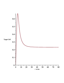
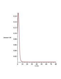
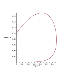
Figure 1: Linear Growth Pattern; d=1.0, r=0.701, p=0.642, s=1.23, c=1.0, u=v=0, k= 0.9255, m= -0.14

Adding non linearity into simulation setting u=v=1, we increase s (velocity rate of immune cell interaction) to 1.53, the system exhibits oscillation phase even target interaction rate k is low. This is shown in Fig. 1 & 2 where very stable phase trajectory is exhibited. The coexistence of stable pattern of both component is illustrated in Fig. 2. The dynamics follows limit cycle characteristics with negative value of m showing equilibrium point.

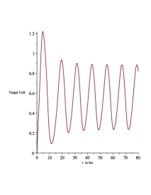
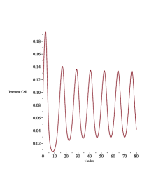
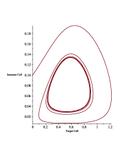
Figure 2: Periodic behavior of growth dynamics ; d=1.0, r=0.701, p=0.642, s=1.56, c=1.0, u=v=1, k= 0.12, m= - 0.12

Our analysis reveals significant role of m in determining stability of the dynamics ( $-0.1<m<0.3$ ). When value of m shifts from this range in either direction, co existence of stable pattern disappears. The oscillation becomes more prominent and stable for longer time when we set v=3 for negative value of m shown in FIG 3.

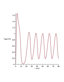
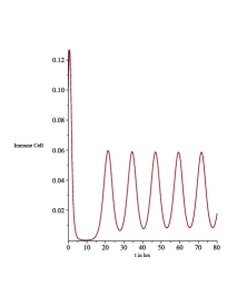
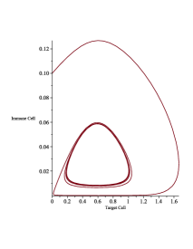
Figure 3: Periodic orbit presence in correlated dynamics ; d=1.0, r=0.701, p=0.642, s=1.56, c=1.0, u=1, v=3, k= 0.12, m= -0.9953

This regime can be recognized as interacting phase of various T/B cell via cytokinase production mechanism in order to achieve immunity for longer period marked by m =- 0.9953. Numerical data exhibits characteristic pattern change after 9-12 hours of the cell infection. Fig. 2 & 3 exhibit characteristic pattern with stable closed trajectory around local attractor. This phase can also be termed as long term antibody production phase and is significant in rubella, german measles, influenza, smallpox etc or any other lethal disease. Oscillation occurs in presence of threshold target cell ($x_{c}+m$) recognized by immune network. This is the case immune system recognizes small presence of target cell through special kind of T cell presence in the system. Existence of multi layer component in immune network in case many lethal diseases such as rubella, HIV are very common. It is evident that ratio of target proliferation $\cfrac{px^{u}}{x^{v}}$ is very dominant to sustain pattern coexistence. Upon increasing a u and v in the network, we observe existence of chaotic phase trajectory shown in FIG 4.

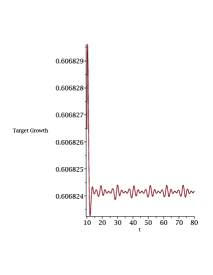
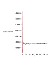
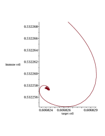
Figure 4: Chaotic phase trajectory ; m = 0.9995 , d=1.0, r=0.701, p=0.642, s=1.72, c=1.0, u=2, v=4, k= 0.265

This kind of oscillatory/chaotic behavior can be termed as indeterministic dynamics where solution can not be obtained following deterministic methods. Stochastic variability of target concentration or strain type within a period of time gives rise to such dynamics.

Moreover, we observe target cell growth becomes zero with very sharp increase of immune cell for $m>0.25$ . This regime can be termed as antibody pattern recognition by immune network shown in FIG 5.

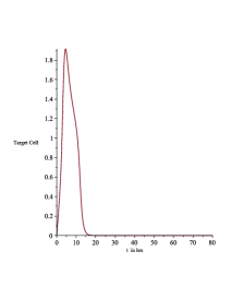
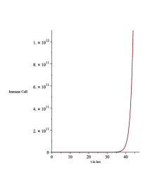
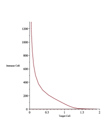
Figure 5: Behavior far away from critical attractor ; $m\geq 0.3$, d=1.0, r=0.701, p=0.642, s=1.72, c=1.0, u=v=1, k= 0.265

The open region in FIG 5 is marked as therapeutic intervention case, often recognized by poor/failed immune system and physics can be explained via uncorrelated/random response of T cell in lymphocyte.

IV Transitive lie algebra method to obtain analtytic solution structure

In order to study symmetry algebra and its role on dynamics, we plan to obtain invariant lie symmetry generator based on Lie symmetry algebra in manifold. The dynamical system

$$\ddot{x}=f(t,x)$$ (13)

will be equivariant under Lie group $\mathrm{g}$ on m (m=2) dimensional manifold M with symmetry group of operator $g^{i}$, then following must be true under periodic temporal symmetry, i.e

$$f(\vec{g}^{i},x,t)={g}^{i}F(x,t+t^{\prime})$$ (14)

for any $t^{\prime}>0$ and the system is called $\mathrm{g}$ symmetric.

In this case, $\mathrm{g}$ acts locally on m - dimensional manifold M. We are interested in the action of $\mathrm{g}$ on p - dimensional sub manifolds $N\subset M$, which we identify as graph of functions in local coordinates. The symmetry and rigidity properties of sub manifolds are all governed by their differential invariants. Here group $\mathrm{g}$ acts continuously on the differential equation. The model considers target invasion with growth rate r and appropriate immune network response given by function g(y) and f(x). If above dynamical pair of equations ( 7- 8) undergo evolution following path of symmetry , it is then necessary to obtain symmetry structure to understand the dynamics. Lie point symmetry and path of transformation is well known to preserve certain dynamical invariant which can be associated with equation of motion, if it exists. Since Lie compact group of continuous point transformation ( continuous group) is special linear group, it can be related to dynamics of holonomic constraints. We assume immune cell responds in a minimal non linear way with n=2 and target stimulation parameter u=v=1. With this assumption, we convert coupled autonomous equations into second order non linear ODE in x(t) as

$$-\cfrac{\ddot{x}(t)}{kx(t)}+\cfrac{{\dot{x}(t)}^{2}}{kx(t)^{2}}=\cfrac{px(t)}{m+1}-\cfrac{px_{0}}{m+1}-\cfrac{x(t)}{{(m+1)}^{2}}+\cfrac{px_{0}}{{(m+1)}^{2}}$$ (15)

$$+\cfrac{sr}{ck}-\cfrac{s}{ck}\cfrac{\dot{x}(t)}{x(t)}-\cfrac{sr^{2}}{c^{2}k^{2}}+\cfrac{2sr}{c^{2}k^{2}}\cfrac{\dot{x}(t)}{x(t)}-\cfrac{s}{k^{2}c^{2}}\cfrac{{\dot{x}(t)}^{2}}{{x(t)}^{2}}-\cfrac{dr}{k}+\cfrac{d}{k}\cfrac{\dot{x}(t)}{x(t)}$$ (16)

which can be expressed as non linear ODE

$$\ddot{x}=f^{k}(t,x(t)^{k}\dot{x}^{k}(t))$$ (17)

$$=\alpha_{2}(t,x){\dot{x}}^{2}+\alpha_{1}(t,x)\dot{x}+\alpha_{0}(,x)x(t)+\cdots$$ (18)

with parameters defined as

$$\alpha_{0}=\cfrac{sr^{2}}{kc^{2}}-\cfrac{sr}{c}-\cfrac{pkx_{0}}{m0^{2}}x^{2}+\cfrac{dr}{k}$$ (19)

$$\alpha_{1}=(\cfrac{s}{c}-\cfrac{2sr}{kc^{2}}-d)$$ (20)

$$\alpha_{2}=(1+\cfrac{s}{kc^{2}})\cfrac{1}{x}$$ (21)

with $x_{0}$ as initial value of x(t). ODE (18) is second order differential equation, non linear in $\dot{x}$ and may be linear/ non linear in x. The idea of linear form of $f_{t}(t,x,\dot{x})$ and related to infinitesimal transformation that would entail dynamical extravagance. Once, analytical structure of the solution is obtained, non linear term can be added into solution.

Through $sl(3,\mathbb{R})$ algebra, any two non commuting, non proportional symmetry generators should follow

$$g_{a}=\xi_{a}\cfrac{\partial}{\partial t}+\eta_{a}\cfrac{\partial}{\partial x}$$ (22)

$$g_{b}=\xi_{b}\cfrac{\partial}{\partial t}+\eta_{b}\cfrac{\partial}{\partial x}$$ (23)

with

$$[g_{a},g_{b}]=\lambda g_{a}$$ (24)

For any physical/biological dynamics represented by second order ODE, differential invariant function of the system is connected to the Lagrangian which describes : A non singular Lagrangian admits a symmetry group having dimension $\leq 3$ . A non singular nth order, $n\geq 2$ admits a symmetry of dimension $\leq n+3$
If $\mathcal{L}(t,x^{n})$ is corresponding g invariant Lagrangian with non vanishing Euler - Lagrange expression $E(\mathcal{L})$, then every g - invariant evolution equation should satisfy

$$\dot{x}=\cfrac{\mathcal{L}}{E(\mathcal{L})}I$$ (25)

where I is an arbitrary differential invariant of the group. If $\mathrm{g}$ represents generators of solvable algebra, corresponding differential invariant can be constructed.

Under one parameter infinitesimal transformation of coordinates (continuous map), we can write

$$\tilde{t}=t+\epsilon\xi(t,x)$$ (26)

$$\tilde{x}=x+\epsilon\eta(t,x)$$ (27)

in the neighborhood of identity with vector field defined

$$g=\xi(t,x)\partial_{t}+\eta(t,x)\partial_{x}$$ (28)

for any $0<\epsilon\ll 1$. The computation of the flow generated by the vector field is often referred to as exponentiation of the vector field under transitive algebra so that each vector in group $\mathrm{g}$ can be integrated through origin in $\mathbb{R}$ . It contains an open neighborhood of the origin and flow.

$$t\rightarrow exp(tg)$$ (29)

is smooth for any vector field. In case of real field $\mathbb{R}^{m}$, constant vector field defined by $g_{a}=\sum a^{i}\cfrac{\partial}{\partial x^{i}}$ with $a=(a^{1},a^{2},\cdots a^{m})$ exponentiates to the group of translation

$$\exp(\epsilon g_{a})=x+\epsilon a$$ (30)

with $x\in{\mathbb{R}}^{m}$. Under continuous symmetry group represented by (26 - 30), mono parametric group generate essential generators for $r\leq 8$. Equation (18 ) under infinitesimal transformation yields

$$\dot{\tilde{x}}=\dot{x}+\epsilon(\eta_{t}+(\eta_{x}-\xi_{t})\dot{x}-\eta_{x}{\dot{x}}^{2}$$ (31)

$$\ddot{\tilde{x}}=\ddot{x}+\epsilon((\eta_{x}-2\xi_{t})-3\xi_{x}\dot{x})\ddot{x}$$ (32)

$$+\epsilon(\eta_{tt}+(2\eta_{xt}-\xi_{tt})\dot{x}$$ (33)

$$+(\eta_{xx}-2\xi_{xt}){\dot{x}}^{2}-\xi_{xx}{\dot{x}}^{3}$$ (34)

for all $(t,x,\dot{x})$. Assuming invariance of (18), we obtain

$$\eta_{tt}+(2\eta_{xt}-\xi_{tt})\dot{x}+(\eta_{xx}-2\xi_{xt}){\dot{x}}^{2}$$ (35)

$$-\xi_{xx}{\dot{x}}^{3}+((\eta_{x}-2\xi_{t})-2\xi_{x}\dot{x})f(t,x,\dot{x})-\xi f_{t}(t,x,\dot{x})-\eta f_{x}(t,x,\dot{x})+(\eta_{t}+(\eta_{x}-\xi_{t})\dot{x}-\xi_{x}{\dot{x}}^{2})f_{\dot{x}}((t,x,\dot{x})\equiv 0$$

Each $\xi$ and $\eta$ here satisfies above relation for higher dimensional algebra. Since, $f(t,x,\dot{x})$ is polynomial in $\dot{x}$, it yields set of PDE s in $\xi$ and $\eta$. Substituting equation (31-32) into (35) and separating null coefficients of powers of $\dot{x}$, we obtain;

$$\xi_{xx}=-\alpha_{2}\xi_{x}$$ (36)

$$\eta_{xx}-2\xi_{xt}-2\alpha_{1}\xi_{x}=\alpha_{2}\eta_{x}+{\alpha_{2}}_{t}\xi+{\alpha_{2}}_{x}\eta$$ (37)

$$2\eta_{xt}-\xi_{tt}-2\alpha_{0}\xi_{x}-\alpha_{1}\xi_{t}-{\alpha_{1}}_{t}\xi-{\alpha_{1}}_{x}\eta=2\alpha_{2}\eta_{t}$$ (38)

$$\eta_{tt}-\alpha_{0}(1\xi_{t}-\eta_{x})-{\alpha_{0}}_{t}\xi-{\alpha_{0}}_{x}\eta_{t}=0$$ (39)

The general solution of this homogeneous linear system can be formally written as a superposition of linearly independent basis solutions $\xi_{a}(t,x)$ and $\eta_{a}(t,x)$ with $a=1,2,\cdots r\leq 8$ following Einstein dummy index

$$\xi(t,x)=x^{a}\xi_{a}(t,x)$$ (40)

$$\eta(t,x)=x^{a}\eta_{a}(t,x)$$ (41)

to construct structure constant. Thus symmetry generator takes the form

$$g_{a}(t,x)=\xi_{a}(t,x)+\eta_{a}(t,x)$$ (42)

subject to Cartan killing condition

$$[g_{a}(t,x),g_{b}(t,x)]={f_{ab}}^{c}g_{c}(t,x)$$ (43)

where ${f_{ab}}^{c}$ is corresponding structure constant .

So, full symmetry group of the differential equation ( 20) should admit following identities davis

$${f_{ab}}^{c}\xi_{c}=[\xi_{a},\xi_{bt}]+[\eta_{a},\xi_{bx}]$$ (44)

$${f_{ab}}^{c}\eta_{c}=[\xi_{a},\eta_{bt}]+[\eta_{a},\eta_{bx}]\$$ (45)

Commutation relations are regular for regular range of values of $\alpha$ s . So, we assume initial data to be regular. Since x= 0 can not be a regular point, we use initial data at regular point is ( t ,x ) = $(t_{0},x_{0})$ to evaluate structure constants. This non singular initial data will uniquely determine structure constant. In order to represent algebra, we introduce parametrization

$$x^{1}=\xi(t_{0},x_{0})x^{2}=\eta(t_{0},x_{0})$$ (46)

$$x^{3}=\xi_{t}(t_{0},x_{0})x^{4}=\eta_{x}(t_{0},x_{0})$$ (47)

$$x^{5}=\eta_{x}(t_{0},x_{0})x^{6}=\eta_{t}(t_{0},x_{0})$$ (48)

$$x^{7}=\cfrac{1}{2}\xi_{tt}(t_{0},x_{0})x^{8}=\cfrac{1}{2}\eta_{xx}(t_{0},x_{0})$$ (49)

According to above relation, we can adopt

$$\xi_{a}(t_{0},x_{0})=\delta_{a1};\hskip 2.0pt\eta_{a}(t_{0},x_{0})=\delta_{a2}$$ (50)

$$\xi_{at}(t_{0},x_{0})=\delta_{a3};\hskip 2.0pt0\eta_{ax}(t_{0},x_{0})=\delta_{a4}$$ (51)

$$\xi_{ax}(t_{0},x_{0})=\delta_{a5};\hskip 2.0pt\;\eta_{at}(t_{0},x_{0})=\delta_{a6}$$ (52)

$$\xi_{att}(t_{0},x_{0})=\delta_{a7};\eta_{axx}(t_{0},x_{0})=2\delta_{a8}$$ (53)

or

$${f_{ab}}^{1}=[\delta_{a1},\delta_{b3}]+[\delta_{a2},\delta_{b5}]$$ (54)

$${f_{ab}}^{2}=[\delta_{a1},\delta_{b6}]+[\delta_{a2},\delta_{b4}]$$ (55)

Because of Lie - Cartan integrability conditions, killing equations ( 50 - 60) satisfy Lie algebra. Solving above equations simultaneously, we find that equation (18) admits sl( 3, $\mathbb{R})$ algebra with following conditions

$$\cfrac{(1-q0^{2})}{m0}=-\cfrac{drm}{kp}$$ (57)

$$\cfrac{s}{kc^{2}}=n$$ (58)

where n presents positive integer. Under transitive algebra, we consider all elements of $g=\sum_{i}c_{i}\cfrac{\partial}{\partial x_{i}}$ and higher order terms of $\mathrm{g}$ for any $x_{i}$.

So, we propose symmetry algebra admitted by non linear ODE (18) as

Proposition 1.

We call this symmetry ”Hidden Dynamical Symmetry ” as this evolves during dynamical evolution in the network system in terms of linear relation between immune growth rate and interaction rate i.e

$$\cfrac{s}{kc^{2}}=n$$ (59)

for any integer value n. We implement most two significant methods symmetric sub algebra to integrate ODE and obtain analytical structure of the solution. The first method is called method to obtain Normal form of generators in the space of variables or quadrature cari . The second method involves normal form of generators in the space of differential invariant function or first integral function pailas . This method can be used when number of symmetries is higher or equal to the order of the equation. It is necessary to use the generators for the integration procedure in a specific order. This depends on the properties of the algebra. When there is a solvable sub algebra of dimension equal to the order of the equation. Integration is performed in correct order and the solution is given solely in terms of quadratures.

The derived algebra of a Lie algebra $(\mathrm{g},[\cdot,\cdot])$ is the sub algebra $g^{1}$ of $\mathrm{g}$ , defined by

$$\mathrm{g}^{1}=[\mathrm{g},\mathrm{g}]$$ (60)

while the derived series is the sequence of Lie sub algebra defined by ${\mathrm{g}}^{0}=\mathrm{g}$ and

$$\mathrm{g}^{(k+1)}=[\mathrm{g}^{k},\mathrm{g}^{k}]$$ (61)

for any $k\in\mathbb{N}$ . Such a sequence satisfies $\mathrm{g}^{(k+1)}\subset\mathrm{g}^{k}$ and the Lie algebra $\mathrm{g}$ is said to be solvable if the derived series eventually arrives at the zero sub algebra. And n- level solvable algebra admits series of invariant sub algebras defined by

$$g\equiv g^{(0)}\supset g^{(1)}\supset g^{(2)}\cdots g^{(n-1)}\supset g^{(n)}\equiv\{0\}$$ (62)

And derived algebra can be constructed by some linearly independent sub set of elements of the commutator of the algebra described by

$$[g^{(1)},g^{(0)}]\subseteq g^{(1)}$$ (63)

Because of above relation, the sub algebra $g^{(1)}$ is an invariant sub algebra of $g^{(0)}$. Since generators have cardinality l= 8, they must follow projective group algebra under $sl(3,\mathcal{R})$ group.

V Normal Form of Generators in the space of Variables

The first integration method to reduce the order of the ODE into quadrature form or equivalently to find out normal form of generators and use those generators to reduce the order of the equation. Under maximal algebra calculation, three generators follow $A_{3,3}$ solvable sub algebra given by

$$[g_{5},g_{7}]=0$$ (64)

$$[g_{5},g_{2}]=g_{5};[g_{7},g_{2}]=g_{7}$$ (65)

which belongs to Weyl group, semi direct product of time dilation and translations $D\otimes x_{2}$. Corresponding ub algebra can be identified as

$$[g^{(1)},g^{(0)}]\subseteq g^{(1)}$$ (66)

with

$$A_{3,3}:=\{g_{5},g_{7};g_{2}\}$$ (67)

Following patera , we compose sub algebra as semi direct sums of a one dimensional sub algebra an abelian ideal with $e_{1},e_{2},e_{3}$ are the bases. For a Lie algebra $\mathcal{g}$ with corresponding Lie group $G=<exp\mathbb{g}>$, the sub algebra can be constructed as semi direct sum of two algebras. The above (64 -67 ) is an two level solvable algebra with $g^{(1)}=\{g_{5},g_{7}\}$ and $g^{(2)}=\{0\}$ . A two level solvable algebra is designated by

$${0}\equiv g^{(2)}\subset g^{(1)}\subset g^{(0)}$$ (68)

Following theorem 3 of pailas , first integration method can be repeated n times upon the following chain of cosets,

$$g^{(n-1)}\equiv{B_{n}}^{(n-1)}\xrightarrow[]{pr}\cdots\xrightarrow[]{pr}{B_{1}}^{0}$$ (69)

where coset is defined between two derived algebras $g^{(i)}$ and $g^{(j)}$ as

$${B_{(}j)}^{(i)}=g^{(i)}-g^{(j)}$$ (70)

Here

$${B_{(2)}}^{(1)}=\{g_{5},g_{7}\}$$ (71)

$$[{B_{(2)}}^{(1)},g^{(0)}]\subseteq{0}$$ (72)

forms abelian algebra. Following theorem 1 pailas , reduced generators form an algebra with structure constants a subset of the original ones such that

$$[{B_{(1)}}^{(0)},{B_{(1)}}^{(0)}]={0}$$ (73)

The two generators of the coset act transitive. Using this, transform generators into normal form. By introducing new coordinates ( T, X) such that T is the independent variable and X is corresponding dependent variable in normal form. as $T=f(t,x)$ and $X=g(t,x)$ , we employ

$$g=\{ag_{5};bg_{7}\}$$ (74)

two dimensional sub algebra such that

$$\tilde{g}T=0,\tilde{g}(XT)=1$$ (75)

holds true. Using twisted Goursat algorithm for decomposable algebra patera , we obtain a= 1, b=3 which yields

$$T=x(t)e^{-\cfrac{(-\alpha_{1}+\sqrt{\alpha_{1}^{2}+4\alpha_{0}})t}{2}}$$ (77)

$$X=\cfrac{x(t)e^{\cfrac{(\alpha-1+\sqrt{{\alpha_{1}}^{2}+4\alpha_{0}})t}{2}}}{4\sqrt{{\alpha_{1}}^{2}+4\alpha_{0}}}$$ (78)

In terms of normal variable ( canonical) ,we obtain ODE

$$({\alpha_{1}}^{2}+4\alpha_{0})T^{3}X_{T,T}X^{2}=0$$ (79)

which is in quadrature form with linear form of solution. Inverse mapping of variables yields solution structure of target component as

$$x_{lin}(t)=\cfrac{C_{2}}{C_{1}e^{\cfrac{\sqrt{{\alpha_{1}}^{2}+4\alpha_{0}}-\alpha_{1})t}{2}}+\cfrac{e^{\cfrac{\sqrt{{\alpha_{1}}^{2}+4\alpha_{0}}-\alpha_{1})t}{2}}}{\sqrt{{\alpha_{1}}^{2}+4\alpha_{0}}}}$$ (80)

with $C_{1},C_{2}$ to be determined from initial conditions.

VI Group Invariant Solution Structure

This method uses differential invariant of the sub group to obtain solution. We use abelian solvable sub algebra

$$[g_{5},g_{7}]=0$$ (81)

under prolonged group to evaluate invariant differential function in the evolution dynamics. We use $g\equiv g_{7}$ here.

$$g^{[1]}\equiv\xi(t,x)\cfrac{\partial}{\partial t}+\eta(t,x)\cfrac{\partial}{\partial x}+\eta^{[1]}\cfrac{\partial}{\partial\dot{x}}$$ (82)

with

$$\xi(t,x)=\cfrac{e^{-(\cfrac{\alpha_{1}+\sqrt{{\alpha-1}^{2}+4\alpha_{0}})t}{2}}}{x(t)}$$ (83)

$$\eta(t,x)=-\cfrac{(\sqrt{{\alpha_{1}}^{2}+4\alpha_{0}}-\alpha_{1})}{2}e^{-(\cfrac{\sqrt{{\alpha_{1}}^{2}+4\alpha_{0}}-\alpha_{1})t}{2}}$$ (84)

$$\eta^{[1]}=\eta_{t}+(\eta_{x}-\xi_{t})\dot{x}-\xi_{x}{\dot{x}}^{2}$$ (85)

with characteristic equation

$$\cfrac{dt}{\xi}=\cfrac{dx}{\eta}=\cfrac{d\dot{x}}{\eta^{[1]}}$$ (86)

which provides two invariant functions , namely $\phi(t,x)$ and $\psi(t,x,\dot{x})$ with

$$g\phi(t,x)=0;$$ (87)

$$g^{[1]}\psi(t,x,\dot{x})=0$$ (88)

$$g^{[2]}\cfrac{d\psi}{d\phi}=0$$ (89)

We concentrate on the system where number of equations in the system is same as number of dependent variables. That means

$$\cfrac{d}{dt}=\cfrac{\partial}{\partial t}+\dot{x}\cfrac{\partial}{\partial x}+\ddot{x}\cfrac{\partial}{\dot{x}}$$ (90)

Two invariant functions gives relation

$$\cfrac{d\psi}{d\phi}=\cfrac{\psi_{t}}{\phi_{t}}=\cfrac{\psi_{t}+\dot{x}(t)\psi_{x}+f\psi_{\dot{t}}}{\phi_{t}+\dot{x}\phi_{x}}$$ (91)

Implementing equations (82-91), we obtain

$$x_{lin}(t)=\cfrac{\sqrt{{\alpha_{1}}^{2}+4\alpha_{0}}}{C_{2}\sqrt{{\alpha_{1}}^{2}+4\alpha_{0}}-C_{1}e^{-t(\sqrt{{\alpha_{1}}^{2}+4\alpha_{0}})}}e^{\cfrac{(-\alpha_{1}+\sqrt{{\alpha_{1}}^{2}+4\alpha_{0}})t}{2}}$$ (92)

where $C_{1}$ and $C_{2}$ will be determined from initial conditions.

VII Numerical Simulation & Results

In the model, parameter u and v play critical role in transition of the dynamics. So, we expand solution around linear (analytical) value by adding nonlinear part in a perturbative way i.e

$$x(t)=x_{lin}(t)+\epsilon f(x,t)+\epsilon^{2}\cfrac{\partial f(x,t)}{\partial t}+\cdots$$ (93)

$$f(x,t)=\cfrac{p{x(t)}^{u}}{m^{v}+{x(t)}^{v}}$$ (94)

Parameter u act as immune stimulation and v as correlation parameter in the network. We keep parameter values same as obtained in dynamical simulation. Following is the result of simulaiton. Linear behavior is exhibited in the simulation using analytical solution without perturbation ( FIG 6). Simulation data from linear structure of the solution exhibit presence of local critical attractor in stable manifold.

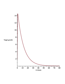
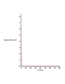
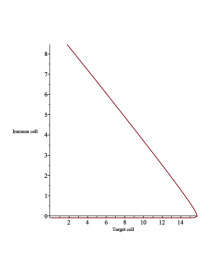
Figure 6: Linear solution behavior based on analytic structure ; d=1.0, r= 0.701, p=0.642, s= 1.23 , m=- 0.14, c=1.0 k =0.93, u=v=0

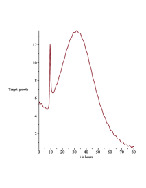
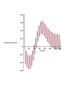
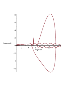
Figure 7: Dynamical behavior with weak correlation u=v=1; d=1.0, r= 0.701, p=0.642, s= 1.23 , m=-0.142, c=1.0 k =0.93, u=v=1

Setting u=1, v=1 and second order perturbation, growth pattern exhibits presence of limit cycle determined by parameter values d=1.0, r=0.7, p=0.642, c=1.0, k=0.25 ( FIG 7). The negative of (m = -0.142) designates attractive phase of dynamics with stable oscillation in closed manifold. The target growth shows consistent increase with numerous small oscillations whereas immune response indicates strong oscillation between 35 and 80 hours. In the simualtion time can be hours or days depending on the intensity of infection. In the first phase, negative oscillatory values of immune density indicates not responding to annihilate target or failure to respond in target invasion. The way immune responds in any case of target invasion in the body is through antibody protein production via CD+8 or CD+4 cytokinase protein. The process of production of these protein involes multi step interaction via several meta stages.

Value u=1, v=3 indicates strong correlation between immune and target dynamics within local domain [FIG 8]. Our simulation reflects chaotic correlated dynamics between two components using second order perturbation. This shows the role of parameter v as correlation in non linear growth dynamics.

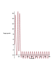
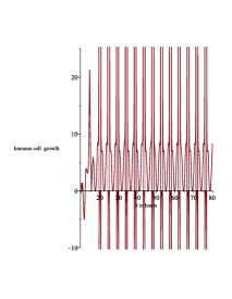
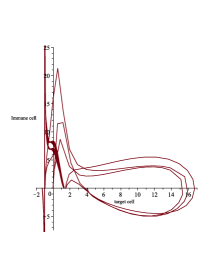
Figure 8: Chaotic behavior of strongly correlated dynamics; d=1.0, r=0.701, p=0.642, s=1.634 , c=1.0, k=0.15, m= -0.13

Under second order perturbation, pattern behavior shifts away from critical attractor designated by positive value of m ($m>0.25$). As a result, phase trajectory becomes open manifold shown in FIG 9 (therapeutic intervention phase). Existence of open manifold case [FIG 9] with low immune cell growth indicates that disease persists and requires therapeutic intervention. his region is also viable for adaptive immunity in case of lethal infection. The parameter value $m\geq 0.25$ plays significant role in development of adaptive immunity which is noted by certain T - cell proliferation through antigen production. This feature is prominent in both approaches. The parameter m here plays significant role via antigen production in case of adaptive immunity. The existence of continuous oscillation or unstable dynamics is noted far away from stable equilibrium ( k= 3.4189 ) when we increase death rate of immune cell d= 1.18 . When we set parameter values v=2.0 ,m=0.3, second order perturbation simualtion of target growth exhibits steady positive for longer time period with maximum value around 40 hours. Positive value of m drives the system away from closed manifold. Immune growth pattern within 30 hours of infection can not compete with target and then starts target annihilation process between 40 and 80 hours after first infection.

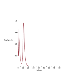
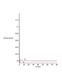
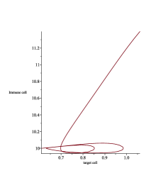
Figure 9: Pattern behavior far away from critical attractor ; $m\geq 0.25$, d=1., r= 0.701, p=0.652, s= 1.625 ,c=1.0, u=1.0 , v=3.0, k= 0.254

VIII Appendix

Table 1: Symmetry Generator following sl( 3, $\mathbb{R}$ ) sub algebra of the ODE

$g_{1}$	$\partial_{t}$
$g_{2}$	$x(t)\partial_{x}$
$g_{3}$	- $x(t)^{2}e^{(\cfrac{\alpha_{1}+\sqrt{{\alpha_{1}}^{2}+4\alpha_{0}})t}{2}}\partial_{x}$
$g_{4}$	$x(t)^{2}e^{(-\cfrac{\alpha_{1}-\sqrt{{\alpha_{1}}^{2}+4\alpha_{0}})t}{2}}\partial_{x}$
$g_{5}$	$\cfrac{e^{(\cfrac{\alpha_{1}-\sqrt{{\alpha_{1}}^{2}+4\alpha_{0}})t}{2}}}{x(t)}\partial_{t}+\cfrac{(\alpha_{1}+\sqrt{{\alpha_{1}}^{2}+4\alpha_{0}})}{2}e^{-(\cfrac{+\sqrt{{\alpha_{1}}^{2}+4\alpha_{0}}-\alpha_{1})t}{2}}\partial_{x}$
$g_{7}$	$\cfrac{e^{-(\cfrac{\alpha_{1}+\sqrt{{\alpha-1}^{2}+4\alpha_{0}})t}{2}}}{x(t)}\partial_{t}-\cfrac{(\sqrt{{\alpha_{1}}^{2}+4\alpha_{0}}-\alpha_{1})}{2}e^{-(\cfrac{\sqrt{{\alpha_{1}}^{2}+4\alpha_{0}}-\alpha_{1})t}{2}}\partial_{x}$

Table 2: Model parameter values for primary/secondary /therapeutic Intervention

n	u	v	r	k	p	s	m	Phase
1	1	1	0.7	0.12	0.642	1.23	0.2	Linear
3	1	2	0.701	0.12	0.642	1.56	-0.13	Periodic
3	1	3	0.702	0.265	0.642	1.65	0.26	Far away from critical attractor

IX Acknowlegment

R. Dutta is thankful to Department of Mathematics for computation support.

X Financial Support

This research received no specific grant from any funding agency, commercial or nonprofit sectors.

XI Conflict of Interests Statement

The authors have no conflicts of interest to disclose.

XII Ethical Statement

This research did not required ethical approval.