Smoothed Gradient Clipping and Error Feedback for Distributed Optimization under Heavy-Tailed Noise

Abstract

Motivated by understanding and analysis of large-scale machine learning under heavy-tailed gradient noise, we study distributed optimization with gradient clipping, i.e., in which certain clipping operators are applied to the gradients or gradient estimates computed from local clients prior to further processing. While vanilla gradient clipping has proven effective in mitigating the impact of heavy-tailed gradient noises in non-distributed setups, it incurs bias that causes convergence issues in heterogeneous distributed settings. To address the inherent bias introduced by gradient clipping, we develop a smoothed clipping operator, and propose a distributed gradient method equipped with an error feedback mechanism, i.e., the clipping operator is applied on the difference between some local gradient estimator and local stochastic gradient. We establish that, for the first time in the strongly convex setting with heavy-tailed gradient noises that may not have finite moments of order greater than one, the proposed distributed gradient method’s mean square error (MSE) converges to zero at a rate $\mathcal{O}(1/t^{\iota})$, $\iota\in(0,1/2)$, where the exponent $\iota$ stays bounded away from zero as a function of the problem condition number and the first absolute moment of the noise and, in particular, is shown to be independent of the existence of higher order gradient noise moments $\alpha>1$. Numerical experiments validate our theoretical findings.

1 Introduction

In this paper, we address the problem of heterogeneous distributed optimization under heavy-tailed gradient noise. We consider the setup where a consortium of $n$ clients orchestrated by a server, in which each client $i$ holds a local function $f_{i}$ and has access to its stochastic gradient with heavy-tailed additive noise via a local and private oracle, collectively optimize the aggregated function $f:=(1/n)\sum_{i=1}^{n}f_{i}$.

The above distributed average-cost minimization formulation has become a key approach in the emerging distributed machine learning paradigm [2, 3], as a prominent method of handling possibly distributed large-scale modern machine learning models and datasets. Intensive research efforts along this direction have yielded algorithms and analyses under various randomness and heterogeneity arising from local functions [4, 5], network environments, client selection [6], and availability [7], and more. Most prior arts focus on gradient noise with bounded variance, which includes some heavy-tailed distributions such as log-normal and Weibull, but limited investigations have been dedicated to distributed stochastic optimization under heavy-tailed gradient noise without the bounded variance assumption. It is well known that classical centralized and distributed stochastic optimization procedures are likely to suffer from instability and divergence in the presence of heavy-tailed stochastic gradients (see [8]). Further, in distributed settings, heavy-tailed noises can cause stochastic gradients to vary significantly in magnitude, posing implementation challenges such as directly communicating stochastic gradients with sufficient precision. To mitigate these issues, a distributed gradient clipping based approach that uses appropriately clipped stochastic gradients at the clients to combat heavy-tailed noise has been proposed in recent work [9]. However, in order to establish convergence, [9] assumes that the stochastic gradients have uniformly bounded $\alpha$ moments for some $\alpha\in(1,2]$, which essentially implies the restrictive condition of uniformly bounded gradients and noise distributions possessing $\alpha$ moments for some $\alpha>1$. Another concurrent work [10] relaxes the bounded gradient condition but still assumes bounded $\alpha$ moment on gradient noises for $\alpha\in(1,2]$. The goal of this work is to relax both two requirements: in particular, we relax the bounded gradient assumption (that enables us to deal with scenarios such as strongly convex costs) and, instead of requiring a uniform $\alpha\in(1,2]$ moment bound on the clients’ stochastic gradients, we only assume that the gradient noises have bounded first absolute moments, i.e., $\alpha=1$.

The study of heavy-tailed gradient noise is motivated by empirical evidence arising in the training of deep learning models [11, 12, 13, 14], for example, the distribution of the gradient noise arising in the training of attention models resembles a Levy $\alpha$-stable distribution that has unbounded variance. In addition, there is evidence that heavy-tailed noise can be induced by distributed machine learning systems with heterogeneous datasets that are not independently and identically distributed (i.i.d.) [9]. Recently, there have been significant advances in developing algorithms and analyses for non-distributed stochastic optimization under certain variants of heavy-tailed noise. The work [13] analyzes clipped stochastic gradient descent (SGD) and establishes convergence rates in the mean-squared sense under gradient noise with bounded $\alpha$-moment, $\alpha\in(1,2]$, and [11] shows mean-squared convergence of vanilla SGD under heavy-tailed $\alpha$-stable distribution. More related to this work, in [8], the authors also assume heavy-tailed settings in which the gradient noise has bounded first absolute moment (and possibly no moment of order strictly greater than one), and introduce a general analytical framework for nonlinear SGD which subsumes popular choices such normalized gradient descent, clipped gradient descent, quantized gradient, etc. Notably, besides mean-squared error (MSE) convergence, [8] also establishes almost sure convergence and asymptotic normality. In comparison, our work considers a distributed setup and focuses on MSE convergence analysis of a specially crafted distributed nonlinear SGD variant that leverages a smoothed gradient clipping operator and an error feedback mechanism to tackle the challenges arising from heavy-tailed client stochastic gradients and client heterogeneity. In terms of error analysis, there is also a growing interest in deriving high-probability rates that logarithmically depend on the confidence level under heavy-tailed gradients for clipped SGD type methods [15, 16, 17, 18, 19, 20, 21, 22]. We defer this discussion to Section 1.2.

While the gradient clipping and related techniques are utilized in various scenarios [13, 18, 19], the lack of convergence analysis for distributed optimization algorithms under heavy-tailed noise that leverage clipping type operators can pertain to, at least partially, the inherent bias introduced by gradient clipping [23] in the stochastic and heterogeneous distributed case [24, 25]. As analyzed in [24, 23], even in the case of deterministic gradients, gradient clipping can lead to non-convergence. In the differential privacy setup where gradient clipping is a commonly used construct, the authors of [20] prove convergence of the distributed gradient clipping by assuming bounded gradient and uniformly bounded gradient dissimilarity, i.e., $\|\nabla f_{i}(\boldsymbol{x})-\nabla f_{j}(\boldsymbol{x})\|\leq c,\ \forall i,j\in[n],\forall\boldsymbol{x}$ for some constant $c$, and the authors of [26] establish convergence by assuming $\|\nabla f_{i}(\boldsymbol{x})-\nabla f(\boldsymbol{x})\|\leq(1/12)\|\nabla f(\boldsymbol{x})\|,\forall i\in[n],\forall\boldsymbol{x}$. In the context of adversarially robust distributed optimization where gradient clipping is adopted to combat adversarial noise, the authors of [27] establish convergence of distributed gradient clipping in a special case where all local convex functions share the same minimizer and $\sum_{i=1}^{n}f_{i}$ is strongly convex. In contrast, this work only assumes bounded gradient heterogeneity at the global optimum, i.e., let $\boldsymbol{x}^{*}=\mathop{\mathrm{arg\,min}}_{\boldsymbol{x}\in\mathbb{R}^{d}}f(\boldsymbol{x})$ we have $\|\nabla f_{i}(\boldsymbol{x}^{*})\|\leq c_{*}$ for each $i\in[n]$ and some constant $c_{*}$. Note that such $c_{*}$ naturally exists given the existence of an optimum. Of particular relevance is the work [28] that proposes to employ an error feedback mechanism to circumvent the issue of unavoidable bias, where the main idea is to clip the difference of some gradient estimators and true gradients. However, [28] only investigates the deterministic gradient case and the stochastic case is still left open. In this work, we adopt a smooth clipping operator [26], complemented by a tailored error feedback mechanism incorporating carefully crafted weights that enables us to cope with heavy-tailed gradient noise. Similarly, to deal with heavy-tailed noises, a concurrent work [10] employs a certain error feedback mechanism with constant weight, and employs clipping on the discrepancies between local stochastic gradients and certain local estimators. Further discussions on error feedback is deferred to Section 1.2.

1.1 Contributions

Our principal contributions in this work are delineated as follows:

Table 1: A comparison on the assumptions and MSE rates for gradient methods with clipping for strongly convex objective functions.

Methods	Distributed	Unbounded gradient	Noise moment	MSE rates
GClip [13]	✗	✗	$\mathbb{E}\|\boldsymbol{\xi}\|^{\alpha}<\infty$, $\alpha>1$	$\mathcal{O}(1/t^{2-2/\alpha})$
FAT-Clipping-PR [9]	✓	✗	$\mathbb{E}\|\boldsymbol{\xi}\|^{\alpha}<\infty$, $\alpha>1$	$\mathcal{O}(1/t^{2-2/\alpha})$
SClip-EF (Ours)	✓	✓	$\mathbb{E}\|\boldsymbol{\xi}\|^{\alpha}<\infty$, $\alpha\geq 1$	$\mathcal{O}(1/t^{\min(c_{s},1/2)})$ 1

• $c_{s}$ is a constant independent of $\alpha$, and depends on the condition number and the first moment bound on gradient noises.

1. We establish the first MSE convergence rate in heterogeneous distributed stochastic optimization under heavy-tailed gradient noise. Specifically, we address the case where local functions are strongly convex and smooth, subject to heavy-tailed gradient noises that are component-wise symmetric about zero and have first absolute moment. Whereas, the most pertinent work [9] assumes that for some $\alpha\in(1,2],c>0$, $\mathbb{E}\|\nabla f(\boldsymbol{x})+\boldsymbol{\xi}\|^{\alpha}\leq c$ uniformly in $\boldsymbol{x}$, where $\nabla f(\boldsymbol{x})$ denotes gradient and $\boldsymbol{\xi}$ denotes noise that is zero-mean, and shows $\mathcal{O}\big{(}1/t^{2-2/\alpha}\big{)}$ MSE convergence rate. Apart from the restricted bounded gradient condition, the MSE rate $\mathcal{O}\big{(}1/t^{2-2/\alpha}\big{)}$ derived in [9] approaches $\mathcal{O}(1)$ when $\alpha$ approaches 1, rendering it inapplicable in our considered scenario in which no moment greater than $\alpha=1$ is required to exist. The concurrent work [10] relaxes the bounded gradient assumption by clipping some local estimation differences, while still assuming gradient noise with moment $\alpha>1$, and establishes high-probability rates. Our work addresses both limitations with distinct algorithmic constructions and analyses. We establishes a MSE rate $\mathcal{O}(1/t^{\iota})$ for some positive $\iota\in(0,1/2)$ that is independent of the existence of $\alpha$ moments with $\alpha>1$. In particular, we show that $\iota$ can be chosen independent of $\alpha$ and is lower bounded by a positive constant that depends on the problem condition number and the magnitude of the noise first absolute moment. We summarize these comparisons of assumptions and rates in Table 1.

2. To tackle the inherent bias arising from gradient clipping in the stochastic and heterogeneous distributed case, we adopt the algorithmic approach that integrates gradient clipping and error feedback. While the authors of [28] develop the analysis for this approach for deterministic gradient case, in this work we carefully craft accompanying smooth clipping operators and weighted error feedback to mitigate the effect of heavy-tailed noise. This specific design leads to substantial differences in analysis with respect to [28] and constitutes a distinct technical contribution. Further, this algorithmic approach of clipping the gradient estimation errors, rather than stochastic gradients, allows for the relaxation of the bounded $\alpha$-moment assumption in [9] to the case where no moment greater than one is required to exist (see also the discussion after Theorem 1 and the numerical experiments in Section 4.)

1.2 Other related works

High probability convergence. In [15], for (strongly) convex problems on bounded sets, the authors prove high-probability rates for SGD and mirror descent equipped with a gradient truncation operator, where they relax the noise sub-Gaussianity assumption and finite variance. In [17], the authors show accelerated rates for strongly convex functions using proxBoost procedure assuming bounded variance but no sub-Gaussianity. In [18, 19], again assuming bounded variance on gradient noise, the authors prove high-probability rates for accelerated SGD with gradient clipping for (strongly) convex problems. For the case where gradient noise may have unbounded variance, in [20, 21], the authors establish high-probability rates for convex and nonconvex functions further assuming bounded gradients, until recently, the authors of [22] remove the restrictive “bounded gradient” assumption and prove optimal high-probability rates for (strongly) convex functions, as well as rates for nonconvex functions. In [16], leveraging additional structures in gradient noises, the authors propose a nonlinear operator coined smoothed medians of means, and manage to derive high-probability rates independent of noise moment $\alpha$.

Error-feedback. Error feedback [29] is widely used to fix the compression error, from some contractive communication compression, in distributed optimization methods with compression [30, 31]. In a recent work [32], the authors propose a simpler error feedback that achieves fast convergence rate under smooth and heterogeneous local functions. The similarities between the clipping operator and the contractive compression operator is also reflected in the work [28]. SClip-EF also shares similar error feedback algorithmic mechanism, however, SClip-EF uses a specially crafted time-varying clipped version of this feedback using a smooth clipping operator.

1.3 Paper organization

The rest of the paper is organized as follows. In Section 2, we introduce our problem model and assumptions. In Section 3, we develop our algorithm and present the main results. Section 4 demonstrates the effectiveness of our algorithm by a strongly convex example with synthetic data and real-world classification datasets, respectively. Section 5 concludes our paper with some discussions on limitations and directions for future research. We defer the proofs of the main result to the Appendix C.

1.4 Notations

We denote by $[n]$ the set $\{1,2,\ldots,n\}$; by $\mathbb{R}$ and $\mathbb{R}_{+}$, respectively, the set of real numbers and nonnegative real numbers, and by $\mathbb{R}^{d}$ the $d$-dimensional Euclidean space. We use lowercase normal letters for scalars, lowercase boldface letter for vectors, and uppercase boldface letter for matrices. Further, we denote by $x_{i}$ the $i$th component of $\boldsymbol{x}$; by $|\boldsymbol{x}|$ the vector $[|x_{1}|,\ldots,|x_{d}|]^{\top}$ for $\boldsymbol{x}\in\mathbb{R}^{d}$; by $\textsc{Diag}(\boldsymbol{x})$ the diagonal matrix whose diagonal is the argument vector $\boldsymbol{x}$; and by $\boldsymbol{I}$ the identity matrix. Next, we let $\|\boldsymbol{x}\|$ and $\|\boldsymbol{x}\|_{\infty}$ denote the $\ell_{2}$ norm and infinity norm of vector $\boldsymbol{x}$, respectively; and $\|\boldsymbol{X}\|_{2}$ denote the operator norm of $\boldsymbol{X}$. Then, for functions $p(t),q(t)$ in $t$, we have $p(t)=\mathcal{O}(q(t))$ if $\limsup_{t\rightarrow\infty}p(t)/q(t)<\infty$; for event $A$, the indicator function $\mathds{1}_{A}=1$ if event $A$ happens, otherwise $0$; and we use $\mathbb{E}$ for expectation over random events. Finally, any inequality between two vectors, or between a vector and a scalar holds true on a component-wise basis; an inequality between random variables and scalars holds true almost surely; an inequality $\boldsymbol{A}\succeq\boldsymbol{B}$ holds if $\boldsymbol{A}-\boldsymbol{B}$ is positive semidefinite.

2 Problem setup

We consider the distributed minimization problem

$$\min_{\boldsymbol{x}\in\mathbb{R}^{d}}f(\boldsymbol{x})=\frac{1}{n}\sum_{i=1}^{n}f_{i}(\boldsymbol{x}),$$

where each local risk function $f_{i}$ is processed by client $i$. At iteration $t$, each client $i\in[n]$ holds the same decision variable $\boldsymbol{x}^{t}$, and query its local stochastic gradient oracle that returns

$$g_{i}(\boldsymbol{x}^{t})=\nabla f_{i}(\boldsymbol{x}^{t})+\boldsymbol{\xi}_{i}^{t},$$

where $\nabla f_{i}(\boldsymbol{x}^{t})$ denotes the true gradient and $\boldsymbol{\xi}_{i}^{t}$ represents heavy-tailed gradient noise. The clients perform local updates and subsequently the server gathers information from clients to update the global parameter $\boldsymbol{x}^{t}$. Following the update, the server distributes the updated parameter $\boldsymbol{x}^{t+1}$ back to all clients. We next present our technical assumptions.

Assumption 1.

For any client $i\in[n]$, $f_{i}:\mathbb{R}^{d}\rightarrow\mathbb{R}$ is twice continuously differentiable, $\mu$-strongly convex, and $L$-smooth. That is, $\forall\boldsymbol{x}\in\mathbb{R}^{d}$, its Hessian $\nabla^{2}f_{i}(\boldsymbol{x})$ satisfies $\mu\mathbf{I}\preceq\nabla^{2}f_{i}(\boldsymbol{x})\preceq L\mathbf{I}$ for some $L\geq\mu>0$.

Any function $f=(1/n)\sum_{i=1}^{n}f_{i}$ that satisfies the above assumption has a unique minimizer. We make the following assumption on the heterogeneity among local functions.

Assumption 2.

Let $\boldsymbol{x}^{*}:=\mathop{\mathrm{arg\,min}}_{\boldsymbol{x}\in\mathbb{R}^{d}}f(\boldsymbol{x})$. For any client $i\in[n]$, the gradient of local function $f_{i}$ satisfies $\|\nabla f_{i}(\boldsymbol{x}^{*})\|\leq c_{*}$.

Remark 1.

The above quantity measures the gradient heterogeneity at the (global) optimum, and it always naturally holds for any finite datasets. We consider $c_{*}$ as a system parameter and make it an explicit assumption. Other stronger heterogeneity conditions include: uniform gradient heterogeneity, i.e., $\|\nabla f_{i}(\boldsymbol{x})-\nabla f(\boldsymbol{x})\|<c,\ \forall i\in[n],\ \forall\boldsymbol{x}\in\mathbb{R}^{d}$ for some constant $c$, that is often made in related federated learning setups [33, 34]; and uniformly bounded gradient, i.e., $\|\nabla f_{i}(\boldsymbol{x})\|<c,\ \forall i\in[n]$ for some constant $c$ in federated learning setups under heavy-tailed noise [9] and federated learning with differential privacy mechanisms [25]. Note that in federated learning algorithms such as FedAvg [35], bounded heterogeneity is necessitated by the incorporation of multiple local steps, while in distributed gradient methods without multiple local updates such as ours, the heterogeneity condition is at least partially due to the use of nonlinear operators such as clipping for the purpose of combating adversarial attacks [36] or differential privacy [26]. In this work, we use this weaker notion of heterogeneity, and leave the extension with multiple local updates for future work.

Assumption 3.

The sequence of gradient noise vectors $\{\{\boldsymbol{\xi}_{i}^{t}\}_{i\in[n]}\}_{t\geq 0}$ are independent over all iterations $t\geq 0$. For any $t\geq 0,i\in[n]$, we assume that every component of the random vector $\boldsymbol{\xi}_{i}^{t}\in\mathbb{R}^{d}$ has the identical marginal probability density function (pdf) , denoted as $p:\mathbb{R}\rightarrow\mathbb{R}_{+}$, that satisfies:

1. $p$ has bounded first absolute moment, i.e., there exists $c_{n}>0$ such that $\int_{-\infty}^{\infty}|u|p(u)du=c_{n}$;

2. $p$ is symmetric, i.e., $p(u)=p(-u),\forall u\in\mathbb{R}$.

Remark 2.

The conditions specified in Assumption 3 enable the existence of a joint pdf $p:\mathbb{R}^{d}\rightarrow\mathbb{R}_{+}$ for any $\boldsymbol{\xi}_{i}^{t}$. It allows for distinct marginals of the joint noise pdf for each component. Furthermore, imposing a bound on the expected $\ell_{1}$ norm implies a bounded first absolute moment for the marginal pdf of each component. Also, assuming $p(\boldsymbol{u})=p(-\boldsymbol{u}),\forall\boldsymbol{u}\in\mathbb{R}^{d}$ enforces symmetry in the marginal pdf for each component.

Example distributions that satisfy Assumption 3 include light-tailed zero-mean Gaussian distribution, zero-mean Laplace distribution, and also heavy-tailed zero-mean symmetric $\alpha-$stable distribution [37].

Example 1.

For a noise distribution that satisfies our assumptions but not the assumptions used in [9, 22], consider the following pdf (see Figure 1 for plot for $\ln\big{(}\mathbb{P}(u>x)\big{)}$ and its comparison with a Gaussian with the same value of $\int_{-\infty}^{\infty}|u|p(u)du$.),

$$p(u)=\frac{c_{p}}{(u^{2}+2)\ln^{2}(u^{2}+2)},$$ (1)

where $c_{p}:=1/\int_{-\infty}^{\infty}1/[(u^{2}+2)\ln^{2}(u^{2}+2)]du$. We have the following proposition with proofs deferred to Appendix A.

Figure 1: An example of a heavy-tailed distribution.

Proposition 1.

The distribution pdf in Example 1 is heavy-tailed, has bounded first absolute moment, but does not have any moment greater than one.

3 Algorithm and main theorem

In the non-distributed setup, several works including [13, 23, 22, 8] have analyzed the following clipped SGD algorithm over iterates $\boldsymbol{x}^{t}\in\mathbb{R}^{d}$, denoted as GClip (Global Clipping) in [13]:

$$\boldsymbol{x}^{t+1}=\boldsymbol{x}^{t}-\eta\operatorname{\textsf{clip}}_{\lambda}(g(\boldsymbol{x}^{t})),$$ (2)

where $\eta$ is stepsize and

$$\operatorname{\textsf{clip}}_{\lambda}(\boldsymbol{y})=\min(\lambda/\|\boldsymbol{y}\|,1)\boldsymbol{y},\forall\boldsymbol{y}\in\mathbb{R}^{d}.$$ (3)

In GClip, all clients communicate local stochastic gradients to the server and the server performs clipping on their average. In a distributed scenario, each client first clips stochastic gradient before sending it to the server, and this leads to the following update, denoted as FAT-Clipping-PR in [9],

$$\boldsymbol{x}^{t+1}=\boldsymbol{x}^{t}-\frac{\eta}{n}\sum_{i=1}^{n}\operatorname{\textsf{clip}}(g_{i}(\boldsymbol{x}^{t}),\lambda).$$ (4)

However, for any constant $\lambda>0$, GClip can lead to non-convergence due to stochastic bias [23], and FAT-Clipping-PR can fail due to client heterogeneity [24]. In this work, we address these issues by proposing an algorithm that utilizes a Smooth Clipping operator with decaying clipping threshold and a weighted Error Feedback mechanism (SClip-EF).

We design a smooth clipping operator $\Psi_{t}$ that transforms any scalar input $y\in\mathbb{R}$ as

$$\Psi_{t}(y) =\frac{c_{\Psi}}{(t+1)^{5/8}}\frac{y}{\sqrt{y^{2}+\tau(t+1)^{3/4}}},\ c_{\Psi},\tau>0.$$ (5)

Applying $\Psi_{t}$ on each component of $\boldsymbol{y}=[y_{1},\ldots,y_{d}]^{\top}\in\mathbb{R}^{d}$, we have the component-wise clipping operator

$$\Psi_{t}(\boldsymbol{y})=[\Psi_{t}(y_{1}),\ldots,\Psi_{t}(y_{d})]^{\top}.$$ (6)

Then, we estimate the average of the stochastic gradient by the average $(1/n)\sum_{i=1}^{n}\boldsymbol{m}_{i}^{t+1}$. The server broadcasts the current iterate $\boldsymbol{x}^{t}$ to all clients, then on each client $i$, the local gradient estimator $\boldsymbol{m}_{i}^{t}$ follows from a weighted error feedback with smoothed clipping,

$$\boldsymbol{m}_{i}^{t+1} =\beta_{t}\boldsymbol{m}_{i}^{t}+(1-\beta_{t})\Psi_{t}(g_{i}(\boldsymbol{x}^{t})-\boldsymbol{m}_{i}^{t})$$ (7)

$$\beta_{t} =\frac{c_{\beta}}{(t+1)^{5/8}},\ c_{\beta}\in(0,1).$$ (8)

Next, all clients communicate the local estimates $\{\boldsymbol{m}_{i}^{t}\}$ to the server, and we perform the main update on the server,

$$\boldsymbol{x}^{t+1} =\boldsymbol{x}^{t}-\frac{\eta}{n}\sum_{i=1}^{n}\boldsymbol{m}_{i}^{t+1},$$ (9)

We refer to the procedures (5)-(9) as SClip-EF. The main idea of SClip-EF is to clip the differences of the local gradient estimator $\boldsymbol{m}_{i}^{t}$ and the local stochastic gradient $\boldsymbol{g}_{i}(\boldsymbol{x}^{t})$. Since $\boldsymbol{g}_{i}(\boldsymbol{x}^{t})-\boldsymbol{m}_{i}^{t}$ is expected to converge to 0, it enables to use smooth clipping operator $\Psi_{t}$ with decaying threshold. The particular designs of $\beta_{t}$ and $\Psi_{t}$ are from our analyses. SClip-EF is parameterized by constants $\eta,c_{\beta},\tau,c_{\Psi}$ and initialization $\boldsymbol{x}^{0}$. We summarize SClip-EF in Algorithm 8.

Algorithm 1 SClip-EF

0:  $\eta,c_{\beta},\tau,c_{\Psi},\boldsymbol{x}^{0}$, oracle function $g$.

1:  $\boldsymbol{m}_{i}^{0}\leftarrow g_{i}(\boldsymbol{x}^{0}),\forall i=1,\ldots,n$

2:  for $t=0,\ldots,T-1$ do

3:     for $i=1,\ldots,n$ do

4:        $\boldsymbol{m}_{i}^{t+1}\leftarrow\beta_{t}\boldsymbol{m}_{i}^{t}+(1-\beta_{t})\Psi_{t}(g_{i}(\boldsymbol{x}^{t})-\boldsymbol{m}_{i}^{t})$

5:     end for

6:     $\boldsymbol{x}^{t+1}\leftarrow\boldsymbol{x}^{t}-\frac{\eta}{n}\sum_{i=1}^{n}\boldsymbol{m}_{i}^{t+1}$

7:  end for

8:  Return $\boldsymbol{x}^{T}$

Theorem 1.

Suppose Assumption 1, 2 and 3 hold. Take $c_{\beta},c_{\Psi}$ as in (5)(8) and sufficiently large $\tau$. The sequence generated by SClip-EF satisfies $\lim_{t\rightarrow\infty}(t+1)^{\iota}\mathbb{E}\|\boldsymbol{x}^{t}-\boldsymbol{x}^{*}\|^{2}=0$ for some $\iota\in(0,1/2)$.

Theorem 1 establishes the first MSE convergence rate of distributed gradient clipping under heavy-tailed gradient noise. This result significantly relaxes the bounded gradient condition assumed in the most pertinent work [9] by imposing moment bound only on gradient noise instead of stochastic gradients. Further, in contrast to the $\alpha$-moment bound for $\alpha>1$ assumed in [9], Theorem 1 only requires a first absolute moment bound, i.e., $\alpha=1$; additionally, the rate $\mathcal{O}\big{(}1/t^{2-2/\alpha}\big{)}$ obtained in [9] breaks when $\alpha$ approaches 1. Note that although the work [8] also studies the heavy-tailed scenario in centralized settings with only first absolute moment bound requirement, it cannot be directly extended to the distributed case, and the smooth clipping operator designed in our work does not satisfy the assumptions of nonlinearities imposed in [8].

Remark 3 (Dependence conditions).

Note that except temporal mutual dependence, our result does not require that the gradient noise random vectors have mutually independent components, and even does not assume mutual independence between $\boldsymbol{\xi}_{i}^{t},\boldsymbol{\xi}^{t}_{j},\forall i,j\in[n]$ and $i\neq j$.

Remark 4 (Exact convergence rate).

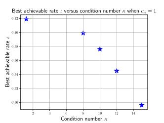
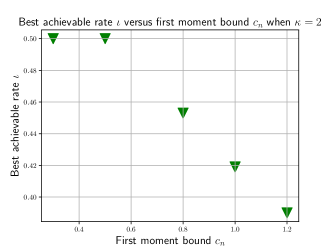
The exact rate $\mathcal{O}(1/t^{\iota})$ depends on the problem condition number $\kappa:=L/\mu$ and the first absolute moment bound $c_{n}$ through the choice of $\tau$. Although the exact rate is not explicitly expressed in terms of problem parameters, we show (see Lemmas 8, 9, 11) that this exponent is lower bounded by a strictly positive function $r(\kappa,c_{n})$ of the condition number and the first absolute noise moment bound $c_{n}$ that stays bounded away from 0 as long as $\kappa$ and $c_{n}$ are finite. In particular, our rate does not depend on higher order moments ($\alpha>1$) of the noise as is the case with [9]. Our results enable computing the MSE rate for any set of parameters and initialization, while the corresponding formula is just not simple/has no closed form available. For example, consider a simple case where $L=500\kappa,\mu=500,c_{*}=1,d=4,\|\boldsymbol{x}^{*}\|=1$, with initialization $\boldsymbol{x}^{0}=\mathbf{0},\max_{i}\|g_{i}(\boldsymbol{x}^{0})\|_{\infty}=1$. We set $\eta=0.9,c_{\beta}=0.1,c_{\Psi}=1$ and tune $\tau$. In the case of $c_{n}=1$, we plot some scatter points of best achievable $\iota$ in our analysis versus $\kappa$ in Figure 2. The plot reveals that ill-conditioned problems generally exhibit slower convergence rates. Additionally, for the case of $\kappa=2$, we depict a scatter plot of the best achievable $\iota$ against the first moment bound $c_{n}$ in Figure 3. The plot naturally demonstrates that larger noise leads to a slowdown in convergence.

Figure 2: Scatter points of best achievable $\iota$ versus $\kappa$.

Figure 3: Scatter points of best achievable $\iota$ versus $c_{n}$.

4 Numerical experiments

4.1 Synthetic data experiments

We simulate a distributed stochastic quadratic minimization problem,

$$\min_{\boldsymbol{x}\in\mathbb{R}^{d}}\frac{1}{n}\sum_{i=1}^{n}\Big{(}\frac{1}{2}\boldsymbol{x}^{\top}\boldsymbol{A}_{i}\boldsymbol{x}+\boldsymbol{b}_{i}^{\top}\boldsymbol{x}\Big{)},$$

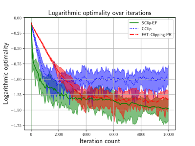
where $d=10$. On each client $i\in[n]$, $\boldsymbol{A}_{i}\in\mathbb{R}^{d\times d}$ is a positive definite matrix, and $\boldsymbol{A}_{i},\boldsymbol{b}_{i}$ are generated at random. The gradient noise follows a truncated version of the heavy-tailed distribution whose pdf is specified by (1) in Example 1. We implement SClip-EF, GClip (as described in (2) (3)), and FAT-Clipping-PR (as described in (4)).

All algorithms are initialized from $\boldsymbol{x}^{0}=0$, and all algorithm parameters are chosen by grid search from certain ranges (as in Figure 4. Further, we implement the noise sampling procedures by discretizing the cumulative distribution function (c.d.f) of (1), and all sampled noises are truncated into the range $[-25,25]$. We note that sampling exactly from the distribution in (1) would not guarantee convergence of GClip, FAT-Clipping-PR as this distribution does not possess any $\alpha$ moment of order $\alpha>1$; with the truncation, technically moments of all orders exist and all the three algorithms are expected to converge, thus enabling us to compare rates.

We compare the logarithmic optimality $\log_{10}\big{(}\|\boldsymbol{x}^{t}-\boldsymbol{x}^{*}\|\big{)}$ of all algorithms in Figure 4, where we plot the trajectory of logarithmic optimality and its mean values over 10 independent runs for the same problem. It can be seen from Figure 4 that SClip-EF converges to the optimum with reasonable fluctuations and converges faster than both GClip and FAT-Clipping-PR, even with a truncated version of a heavy-tailed noise (thus technically guaranteeing the existence of all moments). If one actually samples from (1) (without truncation) that has no moment greater than 1, GClip and FAT-Clipping-PR are not guaranteed to converge as shown in Table 1. Even with noise moments for $\alpha>1$ (as simulated truncated noise), SClip-EF consistently outperforms GClip and FAT-Clipping-PR, showcasing the effectiveness of the smoothed clipping and the error feedback mechanism in dealing with noises with heavy tails. Figure 4 also reveals that SClip-EF and FAT-Clipping-PR converge to a smaller optimum neighborhood compared to the non-distributed GClip, which is perhaps because SClip-EF and FAT-Clipping-PR perform $n$ parallel clippings across the clients and thus able to tame noise better.

Figure 4: $\log_{10}\big{(}\|\boldsymbol{x}^{t}-\boldsymbol{x}^{*}\|\big{)}$ over iterations on synthetic example. SClip-EF: $\eta=1,c_{\beta}=0.5,c_{\Psi}=10,\tau=4$. GClip: $\eta=0.02,\lambda=0.4$. FAT-Clipping-PR: $\eta=0.02$ and $\lambda=0.5$.

4.2 Logistic regression on real-world datasets

To empirically validate the practical effectiveness of SClip-EF, we further conduct a comparative analysis of SClip-EF, Prox-clipped-SGD-shift [10], and FAT-Clipping-PR on distributed real-world datasets Heart, Diabetes and Australian sourced from the LibSVM library [38]. These datasets are evenly distributed across 6 clients. The evaluation focuses on the logistic regression loss function for binary classification. Each client, denoted as $i$, holds a dataset of size $N_{i}$ represented by pairs $\{\boldsymbol{\theta}_{l},\boldsymbol{\xi}_{l}\}$. The local regularized logistic loss function $f_{i}$ for each client is defined as follows:

$$\begin{split}&f_{i}(\boldsymbol{x},\{\boldsymbol{\theta}_{l},\boldsymbol{\xi}_{l}\}_{l=1,\ldots,N_{i}})\\ =\ &\frac{1}{N_{i}}\sum_{l=1}^{N_{i}}\ln\big{(}1+e^{-\boldsymbol{x}^{\top}\boldsymbol{\theta}_{l}\boldsymbol{\xi}_{l}}\big{)}+\frac{\rho}{2}\|\boldsymbol{x}\|_{2}^{2},\end{split}$$ (10)

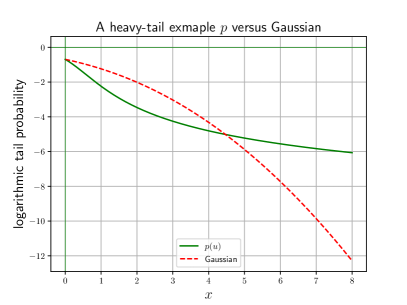
where $\boldsymbol{\theta}_{l}$ represents the feature vector of the $l$-th data point, $\boldsymbol{\xi}_{l}$ corresponds to its binary label in $\{-1,1\}$, and $\rho$ serves as a regularization parameter aimed at preventing overfitting. As previously investigated in [18], when minimizing the loss function (10) on the Diabetes and Australian datasets near the solution $\boldsymbol{x}^{*}$, the norm of gradient noise exhibits outlier values and demonstrates a heavy-tailed behavior, while that in Heart can be well approximated by a Gaussian distribution. See Table 2 for the summary of datasets we used.

	Heart	Diabetes	Australian
Size	270	768	690
Number of features	13	8	13

Table 2: Summary of used datasets

We choose $\rho$ as the reciprocal of the dataset size. Mini-batch stochastic gradients are computed from randomly shuffled sampled data, and we define the process of iterating through the entire dataset as one epoch. All algorithms are initialized from $\boldsymbol{x}^{0}=0$. We first compute a good enough approximation of the optimal solution $f(\boldsymbol{x}^{*})$ in a non-distributed fashion. Then we compare the logarithmic relative optimality $\log_{10}\big{(}(f(\boldsymbol{x}^{t})-f(\boldsymbol{x}^{*}))/(f(\boldsymbol{x}^{0})-f(\boldsymbol{x}^{*}))\big{)}$ of all algorithms in datasets Heart in Figure 5, Diabetes in Figure 6, and Australian in Figure 7. We also provide the algorithmic parameters we used in our experiments after finetuning.

Figure 5: Logarithmic relative optimality over epochs on Heart. SClip-EF: $\eta=1.6,c_{\beta}=0.2,c_{\Psi}=7,\tau=0.004$. Prox-clipped-SGD-shift: stepsize $0.08$, weight for learning shift $0.002$, clipping threshold $0.8$. FAT-Clipping-PR: $\eta=0.05,\lambda=0.85$.

Figure 6: Logarithmic relative optimality over epochs on Diabetes. SClip-EF: $\eta=7,c_{\beta}=0.8,c_{\Psi}=9,\tau=0.006$. Prox-clipped-SGD-shift: stepsize $0.08$, weight for learning shift $0.002$, clipping threshold $1$. FAT-Clipping-PR: $\eta=0.04,\lambda=0.8$.

Figure 7: Logarithmic relative optimality over epochs on Australian. SClip-EF: $\eta=3.6,c_{\beta}=0.4,c_{\Psi}=10,\tau=0.006$. Prox-clipped-SGD-shift: stepsize $0.08$, weight for learning shift $0.003$, clipping threshold $1$. FAT-Clipping-PR: $\eta=0.05,\lambda=1.1$.

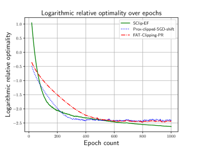
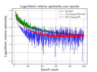
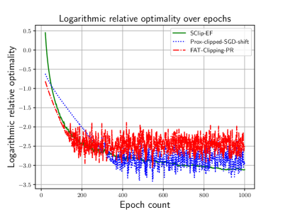
As illustrated in Figure 5, the Heart dataset displays well-behaved gradient noise, with all three algorithms exhibiting smooth trajectories and comparable performance. Conversely, the stochastic gradients in Figures 6 and 7 are more noisy (heavy-tailed). In these cases, SClip-EF demonstrates better stability, achieving comparable performance with Prox-clipped-SGD-shift and FAT-Clipping-PR, and even outperforming them, as observed in Figure 7.

5 Conclusion

In this work, we have studied strongly convex heterogeneous distributed stochastic optimization under heavy-tailed gradient noise. We have proposed SClip-EF, a distributed method that integrates a smooth component-wise clipping operator with decaying clipping thresholds and a weighted feedback mechanism to cope with heavy-tailed stochastic gradients and client heterogeneity. The crux of our approach lies in clipping certain gradient estimation errors rather than the stochastic gradients directly. Under the mild assumption that the gradient noise has only bounded first absolute moment and is (component-wise) symmetric about zero, we have shown that, for the first time in the heterogeneous distributed case, SClip-EF converges to the optimum with a guaranteed sublinear rate. The effectiveness of the proposed algorithm is supported by numerical experiments in both synthetic examples and real-world classification datasets. Future directions include extending the currently analysis to non-convex objective functions and fully distributed server-less networks.

A A heavy-tail example

Consider the following pdf:

$$p(u)=\frac{c_{p}}{(u^{2}+2)\ln^{2}(u^{2}+2)},$$

where $c_{p}:=1/\int_{-\infty}^{\infty}1/[(u^{2}+2)\ln^{2}(u^{2}+2)]du$. The existence of of $c_{p}$ can be readily verified.

Part I. We first show that it is a heavy-tailed distribution. For any positive $x>0$, we have

$$\mathbb{P}(u>x)=\int_{x}^{\infty}\frac{c_{p}}{(u^{2}+2)\ln^{2}(u^{2}+2)}du.$$

Let $w=\ln(u^{2}+2)$, then $u=\sqrt{e^{w}-2}$ and $dw=(2u)du/(u^{2}+2)$. Then,

$$\mathbb{P}(u>x)=\int_{\ln(x^{2}+2)}^{\infty}\frac{c_{p}}{2uw^{2}}dw=\int_{\ln(x^{2}+2)}^{\infty}\frac{c_{p}}{2w^{2}\sqrt{e^{w}-2}}dw\geq\int_{\ln(x^{2}+2)}^{\infty}\frac{c_{p}}{2w^{2}e^{w/2}}dw.$$ (11)

We next bound the rightmost term. Consider any constant $a>0$,

$$\int_{a}^{\infty}\frac{1}{w^{2}e^{w/2}}dw=\frac{e^{-a/2}}{a}-\frac{\Gamma(0,\frac{a}{2})}{2}.$$

Using the Theorem 1.1 in [39], we have

$$\Gamma(0,\frac{a}{2})<e^{-a/2}\ln\big{(}1+\frac{2}{a}\big{)}.$$

It follows that

$$\int_{a}^{\infty}\frac{1}{w^{2}e^{w/2}}dw>\frac{1}{2}e^{-a/2}\big{[}\frac{2}{a}-\ln\big{(}1+\frac{2}{a}\big{)}\big{]}.$$

Note that for any $0<s<3/4$, using Newton-Mercator series we have

$$s-\ln(1+s) =\frac{s^{2}}{2}-\frac{s^{3}}{3}+\frac{s^{4}}{4}-\frac{s^{5}}{5}+\frac{s^{6}}{6}-\frac{s^{7}}{7}\ldots$$

$$=\frac{s^{2}}{2}-\frac{s^{3}}{3}+\frac{s^{4}}{4}\Big{(}1-\frac{4s}{5}\Big{)}+\frac{s^{6}}{6}\Big{(}1-\frac{6s}{7}\Big{)}+\ldots$$

$$\geq\frac{s^{2}}{2}-\frac{s^{3}}{3}$$

$$\geq\frac{s^{2}}{4}+\frac{s^{2}}{4}\Big{(}1-\frac{4s}{3}\Big{)}$$

$$\geq\frac{s^{2}}{4}.$$

In the case that $a>8/3$, from the above two relations we have

$$\int_{a}^{\infty}\frac{1}{w^{2}e^{w/2}}dw>\frac{1}{2a^{2}e^{a/2}}.$$

Combing the above relation with (11) gives that when $\ln(x^{2}+2)>8/3$,

$$\mathbb{P}(u>x)>\frac{c_{p}}{4\sqrt{x^{2}+2}\ln^{2}(x^{2}+2)}\geq\frac{c_{p}}{4(x^{2}+2)^{1/2}(x^{2}+1)^{2}}\geq\frac{c_{p}}{4}(x^{2}+2)^{-5/2}.$$

Then it follows that for any $r>0$, we have

$$\lim_{x\rightarrow\infty}e^{rx}\mathbb{P}(u>x)>\lim_{x\rightarrow\infty}\frac{c_{p}}{4}(x^{2}+2)^{-5/2}e^{rx}=\infty.$$

Part II. We next show that the distribution as in (1) has finite first absolute moment. Again, let $w=\ln(u^{2}+2)$, we have

$$\int_{-\infty}^{\infty}|u|p(u)du=2\int_{0}^{\infty}\frac{c_{p}}{(u^{2}+2)\ln^{2}(u^{2}+2)}du=\int_{\ln 2}^{\infty}\frac{c_{p}}{w^{2}}dw=\frac{c_{p}}{\ln 2}.$$

Part III. For any $\alpha>1$,

$$\int_{-\infty}^{\infty}|u|^{\alpha}p(u)du =2\int_{0}^{\infty}\frac{u^{\alpha-1}u}{(u^{2}+2)\ln^{2}(u^{2}+2)}du$$

$$=\int_{\ln 2}^{\infty}\frac{(e^{w}-2)^{(\alpha-1)/2}}{w^{2}}dw$$

$$>\int_{2\ln 2}^{\infty}\frac{(\frac{e^{w}}{2})^{(\alpha-1)/2}}{w^{2}}dw$$

$$>\frac{1}{2^{(\alpha-1)/2}}\int_{2\ln 2}^{\infty}\frac{1+w(\alpha-1)/2}{w^{2}}dw$$

$$>\frac{\alpha-1}{2^{(\alpha+1)/2}}\int_{2\ln 2}^{\infty}\frac{1}{w}dw$$

$$=\infty.$$

Thus, any moment $\alpha>1$ does not exist.

B Technical Lemmas

The following technical lemmas will be used in our proofs.

Lemma 1 (Theorem 1 in [40]).

Let $\boldsymbol{A}$ and $\boldsymbol{B}$ be positive definite $m$ by $m$ Hermitian matrices with eigenvalues $a_{1}\geq a_{2}\geq\ldots\geq a_{m}$, and $b_{1}\geq b_{2}\geq\ldots\geq b_{m}$, respectively, and let $\boldsymbol{Q}=\boldsymbol{A}\boldsymbol{B}+\boldsymbol{B}\boldsymbol{A}$. Then the minimum eigenvalue $q_{m}$ of $\boldsymbol{Q}$ obeys the inequality,

$$q_{m}\geqslant\min_{\eta=1,m}\left[\frac{a_{\alpha}b_{\alpha}}{2}\left\{\frac{\left(\sqrt{k_{a}}+1\right)^{2}}{\sqrt{k_{a}}}-k_{b}\frac{\left(\sqrt{k_{a}}-1\right)^{2}}{\sqrt{k_{a}}}\right\}\right],$$ (12)

where $k_{a},k_{b}$ are the spectral condition numbers of $\boldsymbol{A}$ and $\boldsymbol{B}$, respectively.

Lemma 2 (Theorem 5.2 in [8], also see Lemma 5 in [41]).

Let $z^{t}$ be a nonnegative (deterministic) sequence satisfying

$$z^{t+1}\leq\left(1-r_{1}^{t}\right)z^{t}+r_{2}^{t},$$

for all $t\geq t^{\prime}$, for some $t^{\prime}\geq 0$, with some $z^{t^{\prime}}\geq 0$. Here $\{r_{1}^{t}\}$ and $\{r_{2}^{t}\}$ are deterministic sequences with $a_{1}/(t+1)^{\delta_{1}}\leq r_{1}^{t}\leq 1$ and $r_{2}^{t}\leq a_{2}/(t+1)^{\delta_{2}}$, with $a_{1},a_{2}>0$ and $\delta_{2}>\delta_{1}>0$. Then the following holds: (1) If $\delta_{1}<1$, then $z^{t}=\mathcal{O}(1/t^{\delta_{2}-\delta_{1}})$; (2) if $\delta_{1}=1$, then $z^{t}=\mathcal{O}(1/t^{\delta_{2}-1})$, provided that $a_{1}>\delta_{2}-\delta_{1}$; (3) if $\delta_{1}=1$ and $a_{1}\leq\delta_{2}-1$, then $z^{t}=\mathcal{O}(1/t^{\zeta})$ for any $\zeta<a_{1}$.

Lemma 3 (Lemma A.1 in [8]).

Consider the (deterministic) sequence

$$v^{t+1}=\left(1-\frac{a_{3}}{(t+1)^{\delta}}\right)v^{t}+\frac{a_{4}}{(t+1)^{\delta}},t\geq t_{0},$$

with $a_{3},a_{4}>0$, $0<\delta\leq 1,t_{0}>0$, and $v^{t_{0}}\geq 0$. Further, assume $t_{0}$ is such that $a_{3}/(t+1)^{\delta}\leq 1$ for all $t\geq t_{0}$. Then $\lim_{t\rightarrow\infty}v^{t}=a_{4}/a_{3}$.

C Proof of Theorem 1

C.1 Preliminaries

Recall that $\boldsymbol{x}^{*}=\mathop{\mathrm{arg\,min}}_{\boldsymbol{x}\in\mathbb{R}^{d}}f(\boldsymbol{x})$. For each $i\in[n]$, we define

$$\boldsymbol{e}_{m,i}^{t}:=\boldsymbol{m}_{i}^{t}-\nabla f_{i}(\boldsymbol{x}^{*}).$$ (13)

For each component $k=1,\ldots,d$, we define

$$\zeta_{k,i}^{t}:=[\nabla f_{i}(\boldsymbol{x}^{t})-\boldsymbol{m}_{i}^{t}]_{k}.$$ (14)

Then, we define the difference between iterate $\boldsymbol{x}^{t}$ and the minimizer as $\boldsymbol{e}_{x}^{t}:=\boldsymbol{x}^{t}-\boldsymbol{x}^{*}$. Since $f_{i}$ is twice continuously differentiable, by mean-value theorem, one can define $\boldsymbol{H}_{f,i}$ as the following,

$$\begin{split}&\nabla f_{i}(\boldsymbol{x}^{t})-\nabla f_{i}(\boldsymbol{x}^{*})\\ =\ &\underbrace{\int_{0}^{1}\big{[}\nabla^{2}f_{i}\big{(}\boldsymbol{x}^{*}+s(\boldsymbol{x}^{t}-\boldsymbol{x}^{*})\big{)}\big{]}ds}_{:=\boldsymbol{H}_{f,i}^{t}}(\boldsymbol{x}^{t}-\boldsymbol{x}^{*})\\ =\ &\boldsymbol{H}_{f,i}^{t}\boldsymbol{e}_{x}^{t}.\end{split}$$ (15)

Recall that we use the function $p$ to denote the pdf of gradient noise. We define the following expectation

$$\Phi_{t}(w):=\int_{-\infty}^{\infty}\Psi_{t}(w+u)p(u)du,\text{ for }w\in\mathbb{R}.$$ (16)

Let $\boldsymbol{w}=[w_{1},\ldots,w_{d}]^{\top}$. We then abuse the notation a little bit and define the column vector $\Phi_{t}(\boldsymbol{w})=[\Phi_{t}(w_{1}),\ldots,\Phi_{t}(w_{d})]^{\top}$. We define the random vector

$$\boldsymbol{\eta}_{i}^{t}:=\Psi_{t}(\nabla f_{i}(\boldsymbol{x}^{t})+\boldsymbol{\xi}^{t}_{i}-\boldsymbol{m}_{i}^{t})-\Phi_{t}(\nabla f_{i}(\boldsymbol{x}^{t})-\boldsymbol{m}_{i}^{t}).$$ (17)

We abstract the history information up to $t-1$, i.e., $\{\boldsymbol{x}_{0},\boldsymbol{\xi}_{i}^{t^{\prime}}\}_{i\in[n],0\leq t^{\prime}\leq t-1}$, into the $\sigma$-algebra $\mathcal{F}_{t}$. Then,

$$\mathbb{E}\big{[}\boldsymbol{\eta}_{i}^{t}\mid\mathcal{F}_{t}\big{]}=0,$$ (18)

and from the definition of $\Psi_{t}$,

$$\|\boldsymbol{\eta}_{i}^{t}\|^{2}\leq\frac{4dc_{\Psi}^{2}}{(t+1)^{5/4}}.$$ (19)

We define a diagonal matrix $\boldsymbol{H}_{\Phi,i}^{t}$ such that

$$\begin{split}\Phi_{t}(\nabla f_{i}(\boldsymbol{x}^{t})-\boldsymbol{m}_{i}^{t})=\boldsymbol{H}_{\Phi,i}^{t}(\nabla f_{i}(\boldsymbol{x}^{t})-\boldsymbol{m}_{i}^{t}).\end{split}$$ (20)

Note that if the $k$th component $\zeta_{k,i}^{t}=[\nabla f_{i}(\boldsymbol{x})-\boldsymbol{m}_{i}^{t}]_{k}$ is zero, then the $k$th diagonal entry of $\boldsymbol{H}_{\Phi,i}^{t}$ can be defined as any quantity.

C.2 Main recursion

Following from the main update (9), and the relation $\sum_{i=1}^{n}\nabla f(\boldsymbol{x}^{*})=0$, one has

$$\boldsymbol{x}^{t+1}-\boldsymbol{x}^{*}$$

$$=\ \boldsymbol{x}^{t}-\boldsymbol{x}^{*}-\frac{\eta}{n}\sum_{i=1}^{n}\boldsymbol{m}_{i}^{t+1}$$

$$\underset{\eqref{eq:mit_update}}{=}\ \boldsymbol{e}_{x}^{t}-\frac{\eta}{n}\sum_{i=1}^{n}\Big{[}\beta_{t}\boldsymbol{m}_{i}^{t}$$

$$\quad+(1-\beta_{t})\Psi_{t}\big{(}\nabla f_{i}(\boldsymbol{x}^{t})+\boldsymbol{\xi}_{i}^{t}-\boldsymbol{m}_{i}^{t}\big{)}\Big{]}$$

$$\underset{\eqref{eq:eta_i_def}}{=}\ \boldsymbol{e}_{x}^{t}-\frac{\eta}{n}\sum_{i=1}^{n}\Big{[}\beta_{t}\boldsymbol{m}_{i}^{t}$$

$$\quad+(1-\beta_{t})\big{(}\Phi_{t}\big{(}\nabla f_{i}(\boldsymbol{x}^{t})-\boldsymbol{m}_{i}^{t}\big{)}+\boldsymbol{\eta}_{i}^{t}\big{)}\Big{]}$$

$$\underset{\eqref{eq:hpsi_i_def}}{=}\ \boldsymbol{e}_{x}^{t}-\frac{\eta\beta_{t}}{n}\sum_{i=1}^{n}\boldsymbol{e}_{m,i}^{t}-\frac{\eta(1-\beta_{t})}{n}\sum_{i=1}^{n}\Big{(}\boldsymbol{\eta}_{i}^{t}+$$

$$\quad\boldsymbol{H}_{\Phi,i}^{t}\big{[}\nabla f_{i}(\boldsymbol{x}^{t})-\nabla f_{i}(\boldsymbol{x}^{*})-(\boldsymbol{m}_{i}^{t}-\boldsymbol{m}_{i}^{*})\big{]}\Big{)}$$

$$\underset{\eqref{eq:emi_def}\eqref{eq:hf_def}}{=}\ \boldsymbol{e}_{x}^{t}-\frac{\eta\beta_{t}}{n}\sum_{i=1}^{n}\boldsymbol{e}_{m,i}^{t}-\frac{\eta(1-\beta_{t})}{n}\sum_{i=1}^{n}\boldsymbol{\eta}_{i}^{t}$$

$$\quad-\frac{\eta(1-\beta_{t})}{n}\sum_{i=1}^{n}\boldsymbol{H}_{\Phi,i}^{t}\big{(}\boldsymbol{H}_{f,i}^{t}\boldsymbol{e}_{x}^{t}-\boldsymbol{e}_{m,i}^{t}\big{)}$$

$$\underset{\eqref{eq:emi_def}}{=}\ \Big{[}\boldsymbol{I}-\frac{\eta(1-\beta_{t})}{n}\sum_{i=1}^{n}\boldsymbol{H}_{\Phi,i}^{t}\boldsymbol{H}_{f,i}^{t}\Big{]}\boldsymbol{e}_{x}^{t}$$

$$\quad-\frac{\eta(1-\beta_{t})}{n}\sum_{i=1}^{n}\boldsymbol{\eta}_{i}^{t}$$

$$\quad-\frac{\eta\beta_{t}}{n}\sum_{i=1}^{n}\boldsymbol{m}_{i}^{t}+\frac{\eta(1-\beta_{t})}{n}\sum_{i=1}^{n}\boldsymbol{H}_{\Phi,i}^{t}\boldsymbol{e}_{m,i}^{t}.$$

We define the following,

$$\boldsymbol{u}_{t}:=\Big{[}\boldsymbol{I}-\frac{\eta(1-\beta_{t})}{n}\sum_{i=1}^{n}\boldsymbol{H}_{\Phi,i}^{t}\boldsymbol{H}_{f,i}^{t}\Big{]}\boldsymbol{e}_{x}^{t},$$ (21)

$$\boldsymbol{v}_{t}:=-\frac{\eta\beta_{t}}{n}\sum_{i=1}^{n}\boldsymbol{m}_{i}^{t},$$ (22)

$$\boldsymbol{z}_{t}:=\frac{\eta(1-\beta_{t})}{n}\sum_{i=1}^{n}\boldsymbol{H}_{\Phi,i}^{t}\boldsymbol{e}_{m,i}^{t}.$$ (23)

Then we can simplify the main recursion as

$$\boldsymbol{e}_{x}^{t+1} =\boldsymbol{u}_{t}+\boldsymbol{v}_{t}+\boldsymbol{z}_{t}-\frac{\eta(1-\beta_{t})}{n}\sum_{i=1}^{n}\boldsymbol{\eta}_{i}^{t}.$$ (24)

We next analyze the convergence of the above recursion. We present some intermediate lemmas, and the proofs of some lemmas are deferred to Appendix C.

C.3 Intermediate lemmas

Lemma 4.

Take $c_{m}:=c_{\beta}\max\big{(}\max_{i}\|g_{i}(\boldsymbol{x}^{0})\|_{\infty},c_{\Psi}\big{)}$ $+c_{\Psi}$. Then, for any $i\in[n],t\geq 1$, $|\boldsymbol{m}_{i}^{t}|\leq c_{m}/t^{5/8}$.

Proof of Lemma 4.

From step 4 in Algorithm 8 and the fact that $|\Psi_{t}|\leq c_{\Psi}/(t+1)^{5/8}$, we have for each $i\in[n]$,

$$|\boldsymbol{m}_{i}^{t+1}|\leq\beta_{t}|\boldsymbol{m}_{i}^{t}|+c_{\Psi}(1-\beta_{t})/\sqrt{t+1},$$ (25)

which leads to

$$|\boldsymbol{m}_{i}^{t+1}|\leq\max(\|\boldsymbol{m}_{i}^{t}\|_{\infty},\ c_{\Psi}/(t+1)^{5/8}).$$ (26)

Since $c_{\Psi}/(t+1)^{5/8}$ is decreasing in $t$, we have

$$|\boldsymbol{m}_{i}^{t}|\leq\max(\|\boldsymbol{m}_{i}^{0}\|_{\infty},c_{\Psi}),\ \forall t\geq 0.$$

Then substituting the above inequality along with $\beta_{t}=c_{\beta}/(t+1)^{5/8}$ into (25) and $\boldsymbol{m}_{i}^{0}=g_{i}(\boldsymbol{x}^{0})$, we have

$$|\boldsymbol{m}_{i}^{t+1}|\leq\frac{c_{\beta}\max(\|g_{i}(\boldsymbol{x}^{0})\|_{\infty},c_{\Psi})}{(t+1)^{5/8}}+\frac{c_{\Psi}}{(t+1)^{5/8}},$$

Taking $c_{m}=c_{\beta}\max\big{(}\max_{i}\|g_{i}(\boldsymbol{x}^{0})\|_{\infty},c_{\Psi}\big{)}+c_{\Psi}$ finishes the proof. ∎

Lemma 5.

Let $c_{x}:=\sqrt{d}\big{(}8\eta c_{m}/3+\|\boldsymbol{x}^{0}\|_{\infty}\big{)}$. Then, for any $t\geq 1$, $\|\boldsymbol{x}^{t}\|\leq c_{x}t^{3/8}$.

Proof of Lemma 5.

From the step 6 in Algorithm 8, we have for $t\geq 0$,

$$\boldsymbol{x}^{t+1}=\boldsymbol{x}^{0}-\sum_{k=0}^{t}\frac{\eta}{n}\sum_{i=1}^{n}\boldsymbol{m}_{i}^{k+1}.$$

Then, by Lemma 4 and triangle inequality, it follows that

$$|\boldsymbol{x}^{t+1}-\boldsymbol{x}^{0}| \leq\sum_{k=0}^{t}\frac{\eta c_{m}}{(k+1)^{5/8}}$$

$$\leq\int_{0}^{t+1}\frac{\eta c_{m}}{s^{5/8}}ds$$

$$=\frac{8\eta c_{m}}{3}(t+1)^{3/8}.$$

Thus, we have

$$|\boldsymbol{x}^{t+1}| \leq|\boldsymbol{x}^{0}|+\frac{8\eta c_{m}}{3}(t+1)^{3/8}$$

$$\leq\Big{(}|\boldsymbol{x}^{0}|+\frac{8\eta c_{m}}{3}\Big{)}(t+1)^{3/8}.$$

Then taking $c_{x}=\sqrt{d}\big{(}\|\boldsymbol{x}^{0}\|_{\infty}+\frac{8\eta c_{m}}{3}\big{)}$ we obtain this lemma. ∎

Lemma 6.

Define $c_{d}:=c_{x}L\sqrt{d}+L\|\boldsymbol{x}^{*}\|+c_{m}+c_{*}.$ Then, for any $t\geq 1,i\in[n],k=1,\ldots,d,$, it satisfies that $|\zeta_{k,i}^{t}|\leq c_{d}t^{3/8}$.

Proof of Lemma 6.

From Lemma 5, we have $\|\boldsymbol{x}^{t}\|\leq c_{x}t^{3/8}$. With the $L$-smoothness in Assumption 1,

$$\begin{split}|\nabla f_{i}(\boldsymbol{x}^{t})-\boldsymbol{m}_{i}^{t}|&\leq|\nabla f(\boldsymbol{x}^{t})-\nabla f(\boldsymbol{x}^{*})-(\boldsymbol{m}_{i}^{t}-\boldsymbol{m}_{i}^{*})|\\ &\leq\|\nabla f(\boldsymbol{x}^{t})-\nabla f(\boldsymbol{x}^{*})\|+|\boldsymbol{m}_{i}^{t}|+|\boldsymbol{m}_{i}^{*}|\\ &\leq L\|\boldsymbol{x}^{t}-\boldsymbol{x}^{*}\|+\frac{c_{m}}{t^{5/8}}+\|\nabla f_{i}(\boldsymbol{x}^{*})\|\\ &\leq L\|\boldsymbol{x}^{t}\|+L\|\boldsymbol{x}^{*}\|+\frac{c_{m}}{t^{5/8}}+c_{*}\\ &\leq c_{x}L\sqrt{d}t^{3/8}+L\|\boldsymbol{x}^{*}\|+c_{m}+c_{*}\\ &\leq\underbrace{\Big{(}c_{x}L\sqrt{d}+L\|\boldsymbol{x}^{*}\|+c_{m}+c_{*}\Big{)}}_{:c_{d}}t^{3/8}.\end{split}$$

∎

Lemma 7.

For any $a>0$, we have $\int_{a}^{\infty}p(u)du\leq c_{n}/(2a)$. For any $0<c_{b}<1$, let $b:=c_{n}/(1-c_{b})$, we have $\int_{-b}^{b}p(u)du\geq c_{b}$.

Proof of Lemma 7.

For any constant $a>0$, by the first absolute moment bound and the symmetry of $p$, we have

$$a\int_{a}^{\infty}p(u)du\leq\int_{a}^{\infty}up(u)du\leq\int_{0}^{\infty}up(u)du=\frac{c_{n}}{2}.$$ (27)

Then it follows that $\int_{a}^{\infty}p(u)du\leq c_{n}/(2a)$. For any constant $0<c_{b}<1$ and its corresponding $b=c_{n}/(1-c_{b})$, by the symmetry of $p$ and (27) one has

$$\int_{-b}^{b}p(u)du=1-2\int_{b}^{\infty}p(u)du\geq c_{b}.$$

∎

Lemma 8.

For any $0<c_{b}<1$, take

$$\tau>\Big{(}8c_{n}^{2}+4\sqrt{4c_{n}^{4}+2c_{b}^{2}c_{d}^{2}c_{n}^{2}+b^{2}}\Big{)}/c_{b}^{2}.$$ (28)

Then, there exist positive constants

$$c_{1}:=c_{b}c_{\Psi}/\sqrt{2c_{d}^{2}+2b^{2}+\tau}-4c_{\Psi}c_{n}/\tau,$$

$$c_{2}:=c_{\Psi}/\sqrt{\tau}+4c_{\Psi}c_{n}/\tau,$$

such that $c_{1}<c_{2}$, and for all $t\geq 1,i\in[n]$, all the diagonal entries of $\boldsymbol{H}_{\Phi,i}^{t}$ fall into the interval $\big{[}c_{1}/(t+1),c_{2}/(t+1)\big{]}$.

Proof of Lemma 8.

Recall that we define in (14) that $\zeta_{k,i}^{t}=[\nabla f_{i}(\boldsymbol{x}^{t})-\boldsymbol{m}_{i}^{t}]_{k}$ for $k=1,\ldots,d$. Suppose $\zeta_{k,i}^{t}\neq 0$. By the definition of $\boldsymbol{H}_{\Phi,i}^{t}$ in (20), its $k$th diagonal entry $[\boldsymbol{H}_{\Phi,i}^{t}]_{kk}$ is

$$\begin{split}\big{[}\boldsymbol{H}_{\Phi,i}^{t}\big{]}_{kk}&=\frac{1}{\zeta_{k,i}^{t}}\int_{-\infty}^{\infty}\frac{c_{\Psi}}{(t+1)^{5/8}}\frac{\zeta_{k,i}^{t}+u}{\sqrt{\big{(}\zeta_{k,i}^{t}+u\big{)}^{2}+\epsilon_{t}}}p(u)du\\ &=\int_{-\infty}^{\infty}\frac{c_{\Psi}}{(t+1)^{5/8}}\frac{p(u)}{\sqrt{\big{(}\zeta_{k,i}^{t}+u\big{)}^{2}+\epsilon_{t}}}du\\ &\quad+\frac{1}{\zeta_{k,i}^{t}}\int_{-\infty}^{\infty}\frac{c_{\Psi}}{(t+1)^{5/8}}\frac{up(u)}{\sqrt{\big{(}\zeta_{k,i}^{t}+u\big{)}^{2}+\epsilon_{t}}}du.\end{split}$$ (29)

If $\zeta_{k,i}^{t}=0$, by the definition of $\boldsymbol{H}_{\Phi,i}^{t}$, we can define $[\boldsymbol{H}_{\Phi}^{t}]_{kk}$ as any quantity, and thus any bounds on (29) will trivially follow. We bound the two summands on the right hand side above one by one. For the first summand, we have the upper bound

$$\ \int_{-\infty}^{\infty}\frac{c_{\Psi}}{(t+1)^{5/8}}\frac{p(u)}{\sqrt{\big{(}\zeta_{k,i}^{t}+u\big{)}^{2}+\epsilon_{t}}}du$$

$$\leq \ \frac{c_{\Psi}}{(t+1)^{5/8}}\frac{1}{\sqrt{\epsilon_{t}}}=\frac{c_{\Psi}}{\sqrt{\tau}(t+1)},$$

and the lower bound

$$\ \int_{-\infty}^{\infty}\frac{c_{\Psi}}{(t+1)^{5/8}}\frac{p(u)}{\sqrt{\big{(}\zeta_{k,i}^{t}+u\big{)}^{2}+\epsilon_{t}}}du$$

$$\geq \ \frac{c_{\Psi}}{(t+1)^{5/8}}\int_{-\infty}^{\infty}\frac{p(u)}{\sqrt{2(\zeta_{k,i}^{t})^{2}+2u^{2}+\epsilon_{t}}}du$$

$$\geq \ \frac{c_{\Psi}}{(t+1)^{5/8}}\int_{-b}^{b}\frac{p(u)}{\sqrt{2(\zeta_{k,i}^{t})^{2}+2u^{2}+\epsilon_{t}}}du$$

$$\geq \ \frac{c_{\Psi}}{(t+1)^{5/8}}\frac{c_{b}}{\sqrt{2c_{d}^{2}(t+1)^{3/4}+2b^{2}+\epsilon_{t}}}$$

$$\geq \ \frac{c_{b}c_{\Psi}}{\sqrt{2c_{d}^{2}+2b^{2}+\tau}}\frac{1}{t+1},$$

where we used that $|\zeta_{k,i}^{t}|\leq c_{d}(t+1)^{3/8}$ from Lemma 6 and $\int_{-b}^{b}p(u)du\geq c_{b}$ from Lemma 7. We next proceed to bound the second summand in (29). We define that

$$P_{k,i}^{t}:=\frac{1}{\sqrt{(\zeta_{k,i}^{t}-u)^{2}+\epsilon_{t}}},\ Q_{k,i}^{t}:=\frac{1}{\sqrt{(\zeta_{k,i}^{t}+u)^{2}+\epsilon_{t}}}.$$ (30)

By the symmetry of $p$, we have that

$$\int_{-\infty}^{\infty}\frac{up(u)}{\sqrt{\big{(}\zeta_{k,i}^{t}+u\big{)}^{2}+\epsilon_{t}}}du=\int_{0}^{\infty}(Q_{k,i}^{t}-P_{k,i}^{t})up(u)du.$$ (31)

We next try to bound $|Q_{k,i}^{t}-P_{k,i}^{t}|$ for the case that $u>0$. If $\zeta_{k,i}>0$, we have

$$\begin{split}&\ |Q_{k,i}^{t}-P_{k,i}^{t}|\\ =&\ \frac{|(Q_{k,i}^{t})^{2}-(P_{k,i}^{t})^{2}|}{Q_{k,i}^{t}+P_{k,i}^{t}}\\ \leq&\ \frac{4|u||\zeta_{k,i}^{t}|}{[(\zeta_{k,i}^{t}-u)^{2}+\epsilon_{t}][(\zeta_{k,i}^{t}+u)^{2}+\epsilon_{t}]}\frac{1}{Q_{k,i}^{t}+P_{k,i}^{t}}\\ \leq&\ \frac{4|u||\zeta_{k,i}^{t}|}{[(\zeta_{k,i}^{t}-u)^{2}+\epsilon_{t}][(\zeta_{k,i}^{t}+u)^{2}+\epsilon_{t}]}\frac{1}{Q_{k,i}^{t}}\\ =&\ \frac{4|u||\zeta_{k,i}^{t}|}{[(\zeta_{k,i}^{t}-u)^{2}+\epsilon_{t}]\sqrt{(\zeta_{k,i}^{t}+u)^{2}+\epsilon_{t}}}\\ \leq&\ \frac{4|u||\zeta_{k,i}^{t}|}{\epsilon_{t}|u|}=\frac{4|\zeta_{k,i}^{t}|}{\epsilon_{t}}.\end{split}$$ (32)

If $\zeta_{k,i}^{t}<0$, similarly we have

$$\begin{split}&\ |Q_{k,i}^{t}-P_{k,i}^{t}|\\ \leq&\ \frac{4|u||\zeta_{k,i}^{t}|}{[(\zeta_{k,i}^{t}-u)^{2}+\epsilon_{t}][(\zeta_{k,i}^{t}+u)^{2}+\epsilon_{t}]}\frac{1}{Q_{k,i}^{k}+P_{k,i}^{k}}\\ \leq&\ \frac{4|u||\zeta_{k,i}^{t}|}{[(\zeta_{k,i}^{t}-u)^{2}+\epsilon_{t}][(\zeta_{k,i}^{t}+u)^{2}+\epsilon_{t}]}\frac{1}{P_{t}^{k}}\\ \leq&\frac{4|u||\zeta_{k,i}^{t}|}{\sqrt{(\zeta_{k,i}^{t}-u)^{2}+\epsilon_{t}}[(\zeta_{k,i}^{t}+u)^{2}+\epsilon_{t}]}\\ \leq&\frac{4|u||\zeta_{k,i}^{t}|}{|u|\epsilon_{t}}=\frac{4|\zeta_{k,i}^{t}|}{\epsilon_{t}}.\end{split}$$ (33)

Thus, for $\zeta_{k,i}^{t}\neq 0$, we have that

$$\begin{split}&\ \frac{1}{\zeta_{k,i}^{t}}\int_{-\infty}^{\infty}\frac{c_{\Psi}}{(t+1)^{5/8}}\frac{up(u)}{\sqrt{\big{(}\zeta_{k,i}^{t}+u\big{)}^{2}+\epsilon_{t}}}du\\ \leq&\ \frac{c_{\Psi}}{|\zeta_{k,i}^{t}|(t+1)^{5/8}}\int_{0}^{\infty}|Q_{k,i}^{t}-P_{k,i}^{t}||u|p(u)du\\ \leq&\ \frac{4c_{\Psi}c_{n}}{\tau(t+1)^{11/8}},\end{split}$$ (34)

where we used the first absolute moment bound in Assumption 3 and (31)(LABEL:eq:pq2)(LABEL:eq:pq3). Therefore, we have that for $\zeta_{k,i}^{t}\neq 0$, it satisfies that

$$\begin{split}[\boldsymbol{H}_{\Phi,i}^{t}]_{kk}&\geq\frac{c_{b}c_{\Psi}}{\sqrt{2c_{d}^{2}+2b^{2}+\tau}}\frac{1}{t+1}-\frac{4c_{\Psi}c_{n}}{\tau(t+1)^{11/8}}\\ &=\frac{1}{t+1}\Big{(}\frac{c_{b}c_{\Psi}}{\sqrt{2c_{d}^{2}+2b^{2}+\tau}}-\frac{4c_{\Psi}c_{n}}{\tau(t+1)^{3/8}}\Big{)}\\ &\geq\frac{1}{t+1}\Big{(}\frac{c_{b}c_{\Psi}}{\sqrt{2c_{d}^{2}+2b^{2}+\tau}}-\frac{4c_{\Psi}c_{n}}{\tau}\Big{)},\end{split}$$ (35)

and

$$\begin{split}[\boldsymbol{H}_{\Phi,i}^{t}]_{kk}&\leq\frac{c_{\Psi}}{\sqrt{\tau}}\frac{1}{t+1}+\frac{4c_{\Psi}c_{n}}{\tau(t+1)^{11/8}}\\ &=\frac{1}{t+1}\Big{(}\frac{c_{\Psi}}{\sqrt{\tau}}+\frac{4c_{\Psi}c_{n}}{\tau(t+1)^{3/8}}\Big{)}\\ &\leq\frac{1}{t+1}\Big{(}\frac{c_{\Psi}}{\sqrt{\tau}}+\frac{4c_{\Psi}c_{n}}{\tau}\Big{)}.\end{split}$$ (36)

We take

$$\tau>\Big{(}8c_{n}^{2}+4\sqrt{4c_{n}^{4}+2c_{b}^{2}c_{n}^{2}(c_{d}^{2}+b^{2})}\Big{)}/c_{b}^{2},$$

to ensure that

$$c_{1}:=\frac{c_{b}c_{\Psi}}{\sqrt{2c_{d}^{2}+2b^{2}+\tau}}-\frac{4c_{\Psi}c_{n}}{\tau}>0,$$

and we also define

$$c_{2}:=\frac{c_{\Psi}}{\sqrt{\tau}}+\frac{4c_{\Psi}c_{n}}{\tau}.$$

It is straightforward to verify that $c_{1}<c_{2}$. From (35) (36) we conclude that for all $t\geq 1$, and $k=1,\ldots,d$,

$$\frac{c_{1}}{t+1}\leq[\boldsymbol{H}_{\Phi,i}^{t}]_{kk}\leq\frac{c_{2}}{t+1}.$$

∎

Lemma 9.

Let $\boldsymbol{S}_{t}=\boldsymbol{I}-\frac{\eta(1-\beta_{t})}{n}\sum_{i=1}^{n}\boldsymbol{H}_{\Phi,i}^{t}\boldsymbol{H}_{f,i}^{t}$. If $\kappa>1$, we use $c_{b}$ such that

$$\Big{(}\frac{\kappa-1}{\kappa+\sqrt{2\kappa-1}}\Big{)}^{2}<c_{b}<1,$$ (37)

and take $\tau$ large enough such that

$$\frac{\sqrt{\tau}+4c_{n}}{\frac{c_{b}\tau}{\sqrt{2c_{d}^{2}+2b^{2}+\tau}}-4c_{n}}\leq\Big{(}\frac{\kappa+\sqrt{2\kappa-1}}{\kappa-1}\Big{)}^{2}.$$ (38)

Also, take $\tau$ large enough such that

$$\frac{c_{b}c_{\Psi}}{\sqrt{2c_{d}^{2}+2b^{2}+\tau}}-\frac{4c_{\Psi}c_{n}}{\tau}<\frac{4}{\eta\mu(1-c_{\beta})}.$$ (39)

Define

$$t_{0}:=\frac{2\eta c_{2}^{2}L^{2}}{c_{1}\mu(1-c_{\beta})}-1,\ c_{s}:=\frac{\eta c_{1}\mu(1-c_{\beta})}{4}.$$

Then $0<c_{s}<1$ and $\forall t\geq t_{0}$, $\|\boldsymbol{S}_{t}\|_{2}\leq 1-c_{s}/(t+1)$.

Proof of Lemma 9.

Note that $\boldsymbol{H}_{\Phi,i}$ is diagonal matrix and $\boldsymbol{H}_{f,i}$ is symmetric. One has

$$\boldsymbol{S}_{t}^{\top}\boldsymbol{S}_{t} =\boldsymbol{I}-\frac{\eta(1-\beta_{t})}{n}\sum_{i=1}^{n}\Big{(}\boldsymbol{H}_{\Phi,i}^{t}\boldsymbol{H}_{f,i}^{t}+\boldsymbol{H}_{f,i}^{t}\boldsymbol{H}_{\Phi,i}^{t}\Big{)}$$

$$\quad+\eta^{2}(1-\beta_{t})^{2}\Big{(}\frac{1}{n}\sum_{i=1}^{n}\boldsymbol{H}_{f,i}^{t}\boldsymbol{H}_{\Phi,i}^{t}\Big{)}\Big{(}\frac{1}{n}\sum_{i=1}^{n}\boldsymbol{H}_{\Phi,i}^{t}\boldsymbol{H}_{f,i}^{t}\Big{)}.$$

Part I. From Lemma 8 and $L$-smoothness from Assumption 1, we have

$$\begin{split}&\ \lambda_{\max}\Big{(}\Big{(}\frac{1}{n}\sum_{i=1}^{n}\boldsymbol{H}_{f,i}^{t}\boldsymbol{H}_{\Phi,i}^{t}\Big{)}\Big{(}\frac{1}{n}\sum_{i=1}^{n}\boldsymbol{H}_{\Phi,i}^{t}\boldsymbol{H}_{f,i}^{t}\Big{)}\Big{)}\\ =&\ \Big{\|}\frac{1}{n}\sum_{i=1}^{n}\boldsymbol{H}_{\Phi,i}^{t}\boldsymbol{H}_{f,i}^{t}\Big{\|}_{2}^{2}\\ \leq&\ \Big{(}\frac{1}{n}\sum_{i=1}^{n}\|\boldsymbol{H}_{\Phi,i}^{t}\|_{2}\|\boldsymbol{H}_{f,i}^{t}\|_{2}\Big{)}^{2}\\ \leq&\ \frac{c_{2}^{2}L^{2}}{(t+1)^{2}},\end{split}$$ (40)

where we used that $\boldsymbol{H}_{f,i}$ is positive semi-definite so $\|\boldsymbol{H}_{f,i}\|_{2}\leq L$.

Part II. We next bound $\lambda_{\min}(\frac{1}{n}\sum_{i=1}^{n}(\boldsymbol{H}_{f,i}^{t}\boldsymbol{H}_{\Phi,i}^{t}+\boldsymbol{H}_{\Phi,i}^{t}\boldsymbol{H}_{f,i}^{t}))$ for any $i\in[n]$. Using the notations as in Lemma 1, let $\boldsymbol{A}=\boldsymbol{H}_{\Phi,i}^{t},\boldsymbol{B}=\boldsymbol{H}_{f,i}^{t}$ and $\boldsymbol{C}=\boldsymbol{A}\boldsymbol{B}$. Then, we have

$$1\leq k_{a}\leq\frac{c_{2}}{c_{1}},\ 1\leq k_{b}\leq\kappa.$$ (41)

We next pick $\tau$ such that

$$\Big{(}\sqrt{k_{a}}+1\Big{)}^{2}-k_{b}\Big{(}\sqrt{k_{a}}-1\Big{)}^{2}\geq 2\sqrt{k_{a}}.$$ (42)

Note that when $\kappa=1$, (42) always holds true.. When $\kappa>1$, to enforce (42), it suffices to have

$$\frac{\kappa-\sqrt{2\kappa-1}}{\kappa-1}\leq\sqrt{k_{a}}\leq\frac{\kappa+\sqrt{2\kappa-1}}{\kappa-1}.$$ (43)

Since $\kappa\geq\sqrt{2\kappa-1}>1$, then naturally,

$$0\leq\frac{\kappa-\sqrt{2\kappa-1}}{\kappa-1}<1\leq\sqrt{k_{a}}.$$

Thus, only the right hand side of (43) needs to be enforced. We take $\tau$ so that the following inequality holds,

$$k_{a}\leq\frac{c_{2}}{c_{1}}=\frac{\sqrt{\tau}+4c_{n}}{c_{b}\sqrt{\frac{\tau}{2c_{d}^{2}+2b^{2}+\tau}}\sqrt{\tau}-4c_{n}}\leq\Big{(}\frac{\kappa+\sqrt{2\kappa-1}}{\kappa-1}\Big{)}^{2}$$ (44)

And one can observe that $c_{2}/c_{1}>1/c_{b}$ and when $\tau\rightarrow\infty$, $c_{2}/c_{1}$ asymptotically decreases to $1/c_{b}$. To ensure (44) can be reached by some large enough $\tau$, one needs

$$\frac{1}{c_{b}}<\Big{(}\frac{\kappa+\sqrt{2\kappa-1}}{\kappa-1}\Big{)}^{2}.$$ (45)

The right hand side is strictly larger than $1$ in the case of $\kappa>1$, so the existence of such $0<c_{b}<1$ is justified. Then, in view of (12), the minimum of the right hand side of (12) is attained when $\alpha=m$. And by (42) and Lemma 8, we have

$$\lambda_{\min}(\boldsymbol{H}_{f,i}^{t}\boldsymbol{H}_{\Phi,i}^{t}+\boldsymbol{H}_{\Phi,i}^{t}\boldsymbol{H}_{f,i}^{t})\geq\frac{c_{1}\mu}{t+1}.$$

Since $\boldsymbol{H}_{f,i}^{t}\boldsymbol{H}_{\Phi,i}^{t}+\boldsymbol{H}_{\Phi,i}^{t}\boldsymbol{H}_{f,i}^{t}$ is real symmetric, by Weyl’s theorem [42], we have

$$\ \lambda_{\min}\Big{(}\frac{1}{n}\sum_{i=1}^{n}(\boldsymbol{H}_{f,i}^{t}\boldsymbol{H}_{\Phi,i}^{t}+\boldsymbol{H}_{\Phi,i}^{t}\boldsymbol{H}_{f,i}^{t})\Big{)}\geq\frac{1}{n}\sum_{i=1}^{n}\lambda_{\min}(\boldsymbol{H}_{f,i}^{t}\boldsymbol{H}_{\Phi,i}^{t}+\boldsymbol{H}_{\Phi,i}^{t}\boldsymbol{H}_{f,i}^{t})\geq\frac{c_{1}\mu}{t+1}.$$

It follows that

$$\lambda_{\max}\Big{(}\boldsymbol{I}-\frac{\eta(1-\beta_{t})}{n}\sum_{i=1}^{n}(\boldsymbol{H}_{f,i}^{t}\boldsymbol{H}_{\Phi,i}^{t}+\boldsymbol{H}_{\Phi,i}^{t}\boldsymbol{H}_{f,i}^{t})\Big{)}\leq 1-\frac{\eta c_{1}\mu(1-c_{\beta})}{t+1}.$$

Part III. We next bound $\lambda_{\max}\big{(}\boldsymbol{S}^{\top}\boldsymbol{S}\big{)}$. Again, by Weyl’s theorem, and (LABEL:eq:thrid-eig), we have that for large enough $t$,

$$\begin{aligned} \lambda_{\max}(\boldsymbol{S}^{\top}\boldsymbol{S})&\leq\lambda_{\max}\Big{(}\boldsymbol{I}-\frac{\eta(1-\beta_{t})}{n}\sum_{i=1}^{n}(\boldsymbol{H}_{\Phi,i}^{t}\boldsymbol{H}_{f,i}^{t}+\boldsymbol{H}_{f,i}^{t}\boldsymbol{H}_{\Phi,i}^{t})\Big{)}\\ &\quad+\eta^{2}(1-\beta_{t})^{2}\lambda_{\max}\Big{(}\Big{(}\frac{1}{n}\sum_{i=1}^{n}\boldsymbol{H}_{f,i}^{t}\boldsymbol{H}_{\Phi,i}^{t}\Big{)}\Big{(}\frac{1}{n}\sum_{i=1}^{n}\boldsymbol{H}_{\Phi,i}^{t}\boldsymbol{H}_{f,i}^{t}\Big{)}\Big{)}\\ &\leq 1-\frac{\eta c_{1}\mu(1-c_{\beta})}{t+1}+\frac{\eta^{2}c_{2}^{2}L^{2}}{(t+1)^{2}}\\ &\leq 1-\frac{\eta c_{1}\mu(1-c_{\beta})}{2(t+1)}\\ &\leq\Big{[}1-\frac{\eta c_{1}\mu(1-c_{\beta})}{4(t+1)}\Big{]}^{2},\end{aligned}$$ (46)

where in the third inequality we take $t$ large enough such that that

$$\frac{\eta c_{1}\mu(1-c_{\beta})}{2(t+1)}\geq\frac{\eta^{2}c_{2}^{2}L^{2}}{(t+1)^{2}},$$

which comes down to

$$t\geq t_{0}:=\frac{2\eta c_{2}^{2}L^{2}}{c_{1}\mu(1-c_{\beta})}-1.$$

We define

$$c_{s}:=\eta c_{1}\mu(1-c_{\beta})/4.$$

We take $\tau$ large enough such that

$$\frac{\eta\mu(1-c_{\beta})}{4}\Big{(}\frac{c_{b}c_{\Psi}}{\sqrt{2c_{d}^{2}+2b^{2}+\tau}}-\frac{4c_{\Psi}c_{n}}{\tau}\Big{)}<1.$$

Then, we have $\forall t\geq t_{0},\|\boldsymbol{S}_{t}\|_{2}\leq 1-c_{s}/(t+1)$. ∎

Lemma 10.

There exists some constant $c_{e}$ such that for any $t\geq 1$, $\mathbb{E}\|\boldsymbol{e}_{x}^{t}\|^{2}\leq c_{e}$.

Proof.

Taking conditional expection on the square of (24), and using (18) (19) and Jensen’s inequality,

$$\mathbb{E}\big{[}\|\boldsymbol{e}_{x}^{t+1}\|^{2}\mid\mathcal{F}_{t}\big{]}\leq\|\boldsymbol{u}_{t}+\boldsymbol{v}_{t}+\boldsymbol{z}_{t}\|^{2}+\frac{4d\eta^{2}c_{\Psi}^{2}}{(t+1)^{5/4}}.$$ (47)

By Young’s inequality, we have

$$\begin{split}&\ \|\boldsymbol{u}_{t}+\boldsymbol{v}_{t}+\boldsymbol{z}_{t}\|\\ \leq&\big{(}1+\frac{c_{s}}{t+1}\big{)}\|\boldsymbol{u}_{t}\|^{2}+\big{(}1+\frac{t+1}{c_{s}}\big{)}(2\|\boldsymbol{v}_{t}\|^{2}+2\|\boldsymbol{z}_{t}\|^{2}).\end{split}$$ (48)

With the fact that $0<c_{s}<1$,

$$\begin{split}&\ \Big{(}1+\frac{c_{s}}{t+1}\Big{)}\Big{(}1-\frac{c_{s}}{t+1}\Big{)}^{2}\\ =&\ 1-\frac{c_{s}}{t+1}+\frac{c_{s}^{2}}{(t+1)^{2}}\Big{(}\frac{c_{s}}{t+1}-1\Big{)}\\ \leq&\ 1-\frac{c_{s}}{t+1},\end{split}$$ (49)

by Lemma 9, we have that for $t\geq t_{0}$,

$$\big{(}1+\frac{c_{s}}{t+1}\big{)}\|\boldsymbol{u}_{t}\|^{2}\leq\big{(}1-\frac{c_{s}}{t+1}\big{)}\|\boldsymbol{e}_{x}^{t}\|^{2}.$$ (50)

From Lemma 4 we have $\|\boldsymbol{m}_{i}^{t}\|\leq 2\sqrt{d}c_{m}/(t+1)^{5/8}$, then

$$2\big{(}1+\frac{t+1}{c_{s}}\big{)}\|\boldsymbol{v}_{t}\|^{2}\leq\frac{8d(1+1/c_{s})\eta^{2}c_{\beta}^{2}c_{m}^{2}}{(t+1)^{3/2}}.$$ (51)

From Lemma 4 and Assumption 2 we have

$$\begin{split}\|\boldsymbol{e}_{m,i}^{t}\|=\|\boldsymbol{m}_{i}^{t}-\nabla f_{i}(\boldsymbol{x}^{*})\|&\leq\sqrt{d}(c_{m}+c_{*}).\end{split}$$ (52)

Thus, with Lemma 8, we have

$$2\big{(}1+\frac{t+1}{c_{s}}\big{)}\|\boldsymbol{z}_{t}\|^{2}\leq\frac{2d(1+1/c_{s})\eta^{2}c_{2}^{2}(c_{m}+c_{*})^{2}}{t+1}.$$

Putting the relations above back into (47) we obtain that for $t\geq t_{0}$,

$$\ \mathbb{E}\big{[}\|\boldsymbol{e}_{x}^{t+1}\|^{2}\mid\mathcal{F}_{t}\big{]}$$

$$\leq \ \big{(}1-\frac{c_{s}}{t+1}\big{)}\|\boldsymbol{e}_{x}^{t}\|^{2}+\frac{8d(1+1/c_{s})\eta^{2}c_{\beta}^{2}c_{m}^{2}}{(t+1)^{3/2}}$$

$$\quad+\frac{2d(1+1/c_{s})\eta^{2}c_{2}^{2}(c_{m}+c_{*})^{2}}{t+1}$$

$$\leq \ \big{(}1-\frac{c_{s}}{t+1}\big{)}\|\boldsymbol{e}_{x}^{t}\|^{2}$$

$$\quad+\frac{2d(1+1/c_{s})\eta^{2}[4c_{\beta}^{2}c_{m}^{2}+c_{2}^{2}(c_{m}+c_{*})^{2}]}{t+1}.$$

It follows from the Lemma 3 in Appendix that $\mathbb{E}\|\boldsymbol{e}_{x}^{t}\|^{2}$ is upper bounded by some constant $c_{e}$. ∎

We next compute a tighter bound on $\mathbb{E}\|\boldsymbol{z}_{t}\|^{2}$ by utilizing the boundedness of $\mathbb{E}\|\boldsymbol{e}_{x}^{t+1}\|^{2}$.

Lemma 11.

Take $\tau>2(L+c_{*}+c_{m}\sqrt{d})^{2}+2$. For all $t\geq t_{0}$ as defined in Lemma 9, there exists some constant $c_{z}>0$ such that $\mathbb{E}\|\boldsymbol{z}_{t}\|^{2}\leq c_{z}/(t+1)^{5/2}$.

Proof of Lemma 11.

Similar to the arguments in the proof of Lemma 8, while bounding the diagonal entries of we can assume that $\zeta_{k,i}^{k}\neq 0$ without loss of generality. By the definition of $\boldsymbol{H}_{\Phi,i}^{t}$ in (20), we have that

$$\begin{split}\big{[}\boldsymbol{H}_{\Phi,i}^{t}\big{]}_{kk}&=\frac{1}{\zeta_{k,i}^{t}}\int_{-\infty}^{\infty}\frac{c_{\Psi}}{(t+1)^{5/8}}\frac{\zeta_{k,i}^{t}+u}{\sqrt{\big{(}\zeta_{k,i}^{t}+u\big{)}^{2}+\epsilon_{t}}}p(u)du\\ &=\int_{-\infty}^{\infty}\frac{c_{\Psi}}{(t+1)^{5/8}}\frac{p(u)}{\sqrt{\big{(}\zeta_{k,i}^{t}+u\big{)}^{2}+\epsilon_{t}}}du\\ &\quad+\underbrace{\frac{1}{\zeta_{k,i}^{t}}\int_{-\infty}^{\infty}\frac{c_{\Psi}}{(t+1)^{5/8}}\frac{up(u)}{\sqrt{\big{(}\zeta_{k}^{t}+u\big{)}^{2}+\epsilon_{t}}}du}_{:=[\boldsymbol{U}_{i}^{t}]_{kk}},\end{split}$$ (53)

where we define diagonal matrix $\boldsymbol{U}_{i}^{t}$ whose $k$-th diagonal entry is $[\boldsymbol{U}_{i}]_{kk}$. First, similar to (LABEL:eq:hphi_2nd_bound), from the symmetry and bounded first absolute moment of the distribution of gradient noise $u$, we have that

$$\begin{split}[\boldsymbol{U}_{i}^{t}]_{kk}\leq\frac{4c_{\Psi}c_{n}}{\tau(t+1)^{11/8}}.\end{split}$$ (54)

We next deal with the first term in (53). For any $\omega>0$, if $\|\boldsymbol{e}_{x}^{t}\|=\|\boldsymbol{x}^{t}-\boldsymbol{x}^{*}\|\leq(t+1)^{\omega}$, we have

$$\begin{split}|\zeta_{k,i}^{t}|&=|[\nabla f_{i}(\boldsymbol{x}^{t})-\boldsymbol{m}_{i}^{t}]_{k}|\\ &\leq\|\nabla f_{i}(\boldsymbol{x}^{t})-\nabla f_{i}(\boldsymbol{x}^{*})+\nabla f_{i}(\boldsymbol{x}^{*})-\boldsymbol{m}_{i}^{t}\|\\ &\leq L(t+1)^{\omega}+c_{*}+\sqrt{d}c_{m}/t^{5/8})\\ &\leq\underbrace{(L+c_{*}+\sqrt{d}c_{m})}_{:=c_{3}}(t+1)^{\omega}.\end{split}$$ (55)

From Markov inequality, one has

$$\mathbb{P}\big{(}\|\boldsymbol{e}_{x}^{t}\|\geq(t+1)^{\omega}\big{)}\leq\frac{\mathbb{E}\|\boldsymbol{e}_{x}^{t}\|^{2}}{(t+1)^{2\omega}}\leq\frac{c_{e}}{(t+1)^{2\omega}}.$$ (56)

Now, we focus on bounding $\mathbb{E}\|\boldsymbol{z}_{t}\|^{2}$.

$$\mathbb{E}\|\boldsymbol{z}_{t}\|^{2}=\mathbb{E}\big{[}\|\boldsymbol{z}_{t}\|^{2}\mathds{1}_{\|\boldsymbol{e}_{x}^{t}\|\leq(t+1)^{\omega}}\big{]}+\mathbb{E}\big{[}\|\boldsymbol{z}_{t}\|^{2}\mathds{1}_{\|\boldsymbol{e}_{x}^{t}\|>(t+1)^{\omega}}\big{]}.$$

From Lemma 8 and (52), (56),

$$\mathbb{E}\big{[}\|\boldsymbol{z}_{t}\|^{2}\mathds{1}_{\|\boldsymbol{e}_{x}^{t}\|>(t+1)^{\omega}}\big{]}\leq\frac{c_{e}d\eta^{2}c_{2}^{2}(c_{m}+c_{*})^{2}}{(t+1)^{2+2\omega}}.$$ (57)

Notice that we have

$$\int_{-\infty}^{\infty}\frac{c_{\Psi}}{(t+1)^{5/8}}\frac{p(u)}{\sqrt{(\zeta_{k,i}^{t}+u)^{2}+\epsilon_{t}}}du\leq\frac{c_{\Psi}}{(t+1)^{5/8}}\frac{1}{\sqrt{\epsilon_{t}}}=\frac{c_{\Psi}}{\sqrt{\tau}(t+1)}.$$

Then, we define diagonal matrix

$$\boldsymbol{Q}^{t}:=\textsc{Diag}\big{[}\frac{c_{\Psi}}{\sqrt{\tau}(t+1)},\ldots,\frac{c_{\Psi}}{\sqrt{\tau}(t+1)}\big{]},$$

and define

$$\Delta_{i}^{t}:=\boldsymbol{Q}^{t}-\int_{-\infty}^{\infty}\frac{c_{\Psi}}{(t+1)^{5/8}}\frac{p(u)}{\sqrt{\big{(}\zeta_{k,i}^{t}+u\big{)}^{2}+\epsilon_{t}}}du.$$ (58)

Suppose $\|\boldsymbol{e}_{x}^{t}\|<(t+1)^{\omega}$, from (55) one has

$$\begin{split}&\ \int_{-\infty}^{\infty}\frac{c_{\Psi}}{(t+1)^{5/8}}\frac{p(u)}{\sqrt{\big{(}\zeta_{k,i}^{t}+u\big{)}^{2}+\epsilon_{t}}}du\\ \geq&\ \int_{-\infty}^{\infty}\frac{c_{\Psi}}{(t+1)^{5/8}}\frac{p(u)}{\sqrt{2c_{3}^{2}(t+1)^{2\omega}+2u^{2}+\epsilon_{t}}}du\\ \geq&\ \int_{-(t+1)^{\omega}}^{(t+1)^{\omega}}\frac{c_{\Psi}}{(t+1)^{5/8}}\frac{p(u)}{\sqrt{(2c_{3}^{2}+2)(t+1)^{2\omega}+\epsilon_{t}}}du\\ =&\ \frac{c_{\Psi}}{\sqrt{\tau}(t+1)}\frac{1}{\sqrt{1+\frac{2c_{3}^{2}+2}{\tau(t+1)^{3/4-2\omega}}}}\int_{-(t+1)^{\omega}}^{(t+1)^{\omega}}p(u)du\\ \geq&\frac{c_{\Psi}\big{(}1-2\int_{(t+1)^{\omega}}^{\infty}p(u)du\big{)}}{\sqrt{\tau}(t+1)}\Big{(}1-\frac{2c_{3}^{2}+2}{\tau(t+1)^{3/4-2\omega}}\Big{)}\\ \geq&\frac{c_{\Psi}}{\sqrt{\tau}(t+1)}\Big{[}1-\Big{(}\frac{2c_{3}^{2}+2}{\tau(t+1)^{3/4-2\omega}}+2\int_{(t+1)^{\omega}}^{\infty}p(u)du\big{)}\Big{)}\Big{]},\end{split}$$ (59)

where in the second last inequality we take $\tau>2c_{3}^{2}+2$ and used the fact that for every $0<a<1$,

$$\frac{1}{\sqrt{1+a}}\geq\sqrt{1-a}\geq 1-a.$$ (60)

Combing the relations (58)(59) gives that for each $k=1,\ldots,d$,

$$[\Delta_{i}^{t}]_{kk} \leq\frac{c_{\Psi}}{\sqrt{\tau}(t+1)}\Big{(}\frac{2c_{3}^{2}+2}{\tau(t+1)^{3/4-2\omega}}+2\int_{(t+1)^{\omega}}^{\infty}p(u)du\Big{)}$$

$$\leq\frac{c_{\Psi}}{\sqrt{\tau}(t+1)}\Big{(}\frac{2c_{3}^{2}+2}{\tau(t+1)^{3/4-2\omega}}+\frac{c_{n}}{(t+1)^{\omega}}\Big{)}$$

$$\leq\frac{c_{\Psi}}{\sqrt{\tau}(t+1)}\frac{(2c_{3}^{2}+2)/\tau+c_{n}}{(t+1)^{\min(3/4-2\omega,\ \omega)}},$$

where in the first inequality we used Lemma 7. Then, using that $\sum_{i=1}^{n}\boldsymbol{e}_{m,i}^{t}=\sum_{i=1}^{n}\boldsymbol{m}_{i}^{t}$,

$$\ \mathbb{E}\big{[}\|\boldsymbol{z}_{t}\|^{2}\mathds{1}_{\|\boldsymbol{e}_{x}^{t}\|<(t+1)^{\omega}}\big{]}$$

$$= \ \mathbb{E}\Big{[}\Big{\|}\frac{\eta(1-\beta_{t})}{n}\sum_{i=1}^{n}\big{(}\boldsymbol{Q}^{t}-\Delta_{i}^{t}+\boldsymbol{U}_{i}^{t}\big{)}\boldsymbol{e}_{m,i}^{t}\Big{\|}^{2}\mathds{1}_{\|\boldsymbol{e}_{x}^{t}\|<(t+1)^{\omega}}\Big{]}$$

$$\leq \ 3\eta^{2}\mathbb{E}\Big{[}\mathds{1}_{\|\boldsymbol{e}_{x}^{t}\|<(t+1)^{\omega}}\Big{(}\Big{\|}\frac{\boldsymbol{Q}^{t}}{n}\sum_{i=1}^{n}\boldsymbol{m}_{i}^{t}\Big{\|}^{2}+\Big{\|}\frac{1}{n}\sum_{i=1}^{n}\Delta_{i}^{t}\boldsymbol{e}_{m,i}^{t}\Big{\|}^{2}+\Big{\|}\frac{1}{n}\sum_{i=1}^{n}\boldsymbol{U}_{i}^{t}\boldsymbol{e}_{m,i}^{t}\Big{\|}^{2}\Big{)}\Big{]}$$

$$\leq \ 3\eta^{2}\Big{(}\frac{4dc_{\Psi}^{2}c_{m}^{2}}{\tau(t+1)^{13/4}}+\frac{dc_{\Psi}^{2}((2c_{3}^{2}+2)/\tau+c_{n})^{2}(c_{m}+c_{*})^{2}}{\tau(t+1)^{2+2\min(3/4-2\omega,\ \omega)}}+\frac{16dc_{\Psi}^{2}c_{n}^{2}(c_{m}+c_{*})^{2}}{\tau^{2}(t+1)^{11/4}}\Big{)}.$$

Combing the above relation the (57) we have

$$\mathbb{E}\|\boldsymbol{z}_{t}\|^{2}\leq \ \frac{c_{4}}{(t+1)^{2+2\min(3/4-2\omega,\ \omega)}}+\frac{c_{5}}{(t+1)^{11/4}},$$

for constants $c_{4},c_{5}$ defined as

$$c_{4}:=c_{e}d(c_{m}+c_{*})^{2}\eta^{2}c_{2}^{2}+\frac{3d\eta^{2}c_{\Psi}^{2}((2c_{3}^{2}+2)/\tau+c_{n})^{2}(c_{m}+c_{*})^{2}}{\tau},$$

$$c_{5}:=\frac{12d\eta^{2}c_{\Psi}^{2}c_{m}^{2}}{\tau}+\frac{48d\eta^{2}c_{\Psi}^{2}c_{n}^{2}(c_{m}+c_{*})^{2}}{\tau^{2}}.$$

Take $\omega=1/4$, we have

$$2+2\min(3/4-2\omega,\omega)=\frac{5}{2}<\frac{11}{4}.$$

It follows that for $c_{z}:=c_{4}+c_{5}$,

$$\mathbb{E}\|\boldsymbol{z}_{t}\|^{2}\leq\frac{c_{z}}{(t+1)^{5/2}}.$$

∎

C.4 Proof of main theorem

Proof of Theorem 1.

Taking expectation on both sides of (47), combining (LABEL:eq:uvzsum)-(51) and Lemma 11 gives that for $t\geq t_{0}$,

$$\mathbb{E}\|\boldsymbol{e}_{x}^{t+1}\|^{2} \leq\big{(}1-\frac{c_{s}}{t+1}\big{)}\mathbb{E}\|\boldsymbol{e}_{x}^{t}\|^{2}+\frac{c_{\delta}}{(t+1)^{3/2}},$$

for $c_{\delta}:=8d(1+1/c_{s})\eta^{2}c_{\beta}^{2}c_{m}^{2}+2c_{z}(1+1/c_{s})$. A direct application of Lemma 2 leads to the MSE rate $\mathbb{E}\|\boldsymbol{e}_{x}^{t}\|^{2}=\mathcal{O}\big{(}1/t^{\min(c_{s},1/2)}\big{)}$.

∎

References

- [1] J. Nair, A. Wierman, and B. Zwart, The fundamentals of heavy tails: Properties, emergence, and estimation. Cambridge University Press, 2022, vol. 53.
- [2] T. Li, A. K. Sahu, M. Zaheer, M. Sanjabi, A. Talwalkar, and V. Smith, “Federated optimization in heterogeneous networks,” Proceedings of Machine learning and systems, vol. 2, pp. 429–450, 2020.
- [3] P. Kairouz, H. B. McMahan, B. Avent, A. Bellet, M. Bennis, A. N. Bhagoji, K. Bonawitz, Z. Charles, G. Cormode, R. Cummings et al., “Advances and open problems in federated learning,” Foundations and Trends® in Machine Learning, vol. 14, no. 1–2, pp. 1–210, 2021.
- [4] S. P. Karimireddy, S. Kale, M. Mohri, S. Reddi, S. Stich, and A. T. Suresh, “Scaffold: Stochastic controlled averaging for federated learning,” in International conference on machine learning. PMLR, 2020, pp. 5132–5143.
- [5] J. Wang, Q. Liu, H. Liang, G. Joshi, and H. V. Poor, “Tackling the objective inconsistency problem in heterogeneous federated optimization,” Advances in neural information processing systems, vol. 33, pp. 7611–7623, 2020.
- [6] Y. J. Cho, J. Wang, and G. Joshi, “Towards understanding biased client selection in federated learning,” in International Conference on Artificial Intelligence and Statistics. PMLR, 2022, pp. 10 351–10 375.
- [7] Y. Ruan, X. Zhang, S.-C. Liang, and C. Joe-Wong, “Towards flexible device participation in federated learning,” in International Conference on Artificial Intelligence and Statistics. PMLR, 2021, pp. 3403–3411.
- [8] D. Jakovetić, D. Bajović, A. K. Sahu, S. Kar, N. Milosević, and D. Stamenković, “Nonlinear gradient mappings and stochastic optimization: A general framework with applications to heavy-tail noise,” SIAM Journal on Optimization, vol. 33, no. 2, pp. 394–423, 2023.
- [9] H. Yang, P. Qiu, and J. Liu, “Taming fat-tailed (“heavier-tailed” with potentially infinite variance) noise in federated learning,” Advances in Neural Information Processing Systems, vol. 35, pp. 17 017–17 029, 2022.
- [10] E. Gorbunov, A. Sadiev, M. Danilova, S. Horváth, G. Gidel, P. Dvurechensky, A. Gasnikov, and P. Richtárik, “High-probability convergence for composite and distributed stochastic minimization and variational inequalities with heavy-tailed noise,” arXiv preprint arXiv:2310.01860, 2023.
- [11] U. Şimşekli, M. Gürbüzbalaban, T. H. Nguyen, G. Richard, and L. Sagun, “On the heavy-tailed theory of stochastic gradient descent for deep neural networks,” arXiv preprint arXiv:1912.00018, 2019.
- [12] U. Simsekli, L. Sagun, and M. Gurbuzbalaban, “A tail-index analysis of stochastic gradient noise in deep neural networks,” in International Conference on Machine Learning. PMLR, 2019, pp. 5827–5837.
- [13] J. Zhang, S. P. Karimireddy, A. Veit, S. Kim, S. Reddi, S. Kumar, and S. Sra, “Why are adaptive methods good for attention models?” Advances in Neural Information Processing Systems, vol. 33, pp. 15 383–15 393, 2020.
- [14] M. Gurbuzbalaban, U. Simsekli, and L. Zhu, “The heavy-tail phenomenon in sgd,” in International Conference on Machine Learning. PMLR, 2021, pp. 3964–3975.
- [15] A. V. Nazin, A. S. Nemirovsky, A. B. Tsybakov, and A. B. Juditsky, “Algorithms of robust stochastic optimization based on mirror descent method,” Automation and Remote Control, vol. 80, pp. 1607–1627, 2019.
- [16] N. Puchkin, E. Gorbunov, N. Kutuzov, and A. Gasnikov, “Breaking the heavy-tailed noise barrier in stochastic optimization problems,” arXiv preprint arXiv:2311.04161, 2023.
- [17] D. Davis, D. Drusvyatskiy, L. Xiao, and J. Zhang, “From low probability to high confidence in stochastic convex optimization,” The Journal of Machine Learning Research, vol. 22, no. 1, pp. 2237–2274, 2021.
- [18] E. Gorbunov, M. Danilova, and A. Gasnikov, “Stochastic optimization with heavy-tailed noise via accelerated gradient clipping,” Advances in Neural Information Processing Systems, vol. 33, pp. 15 042–15 053, 2020.
- [19] E. Gorbunov, M. Danilova, I. Shibaev, P. Dvurechensky, and A. Gasnikov, “Near-optimal high probability complexity bounds for non-smooth stochastic optimization with heavy-tailed noise,” arXiv preprint arXiv:2106.05958, 2021.
- [20] J. Zhang and A. Cutkosky, “Parameter-free regret in high probability with heavy tails,” Advances in Neural Information Processing Systems, vol. 35, pp. 8000–8012, 2022.
- [21] A. Cutkosky and H. Mehta, “High-probability bounds for non-convex stochastic optimization with heavy tails,” Advances in Neural Information Processing Systems, vol. 34, pp. 4883–4895, 2021.
- [22] A. Sadiev, M. Danilova, E. Gorbunov, S. Horváth, G. Gidel, P. Dvurechensky, A. Gasnikov, and P. Richtárik, “High-probability bounds for stochastic optimization and variational inequalities: the case of unbounded variance,” arXiv preprint arXiv:2302.00999, 2023.
- [23] A. Koloskova, H. Hendrikx, and S. U. Stich, “Revisiting gradient clipping: Stochastic bias and tight convergence guarantees,” in ICML 2023-40th International Conference on Machine Learning, 2023.
- [24] X. Chen, S. Z. Wu, and M. Hong, “Understanding gradient clipping in private sgd: A geometric perspective,” Advances in Neural Information Processing Systems, vol. 33, pp. 13 773–13 782, 2020.
- [25] X. Zhang, X. Chen, M. Hong, Z. S. Wu, and J. Yi, “Understanding clipping for federated learning: Convergence and client-level differential privacy,” in International Conference on Machine Learning, ICML 2022, 2022.
- [26] B. Li and Y. Chi, “Convergence and privacy of decentralized nonconvex optimization with gradient clipping and communication compression,” arXiv preprint arXiv:2305.09896, 2023.
- [27] S. Yu and S. Kar, “Secure distributed optimization under gradient attacks,” IEEE Transactions on Signal Processing, 2023.
- [28] S. Khirirat, E. Gorbunov, S. Horváth, R. Islamov, F. Karray, and P. Richtárik, “Clip21: Error feedback for gradient clipping,” arXiv preprint arXiv:2305.18929, 2023.
- [29] F. Seide, H. Fu, J. Droppo, G. Li, and D. Yu, “1-bit stochastic gradient descent and its application to data-parallel distributed training of speech dnns,” in Fifteenth annual conference of the international speech communication association, 2014.
- [30] J. Wu, W. Huang, J. Huang, and T. Zhang, “Error compensated quantized sgd and its applications to large-scale distributed optimization,” in International Conference on Machine Learning. PMLR, 2018, pp. 5325–5333.
- [31] S. P. Karimireddy, Q. Rebjock, S. Stich, and M. Jaggi, “Error feedback fixes signsgd and other gradient compression schemes,” in International Conference on Machine Learning. PMLR, 2019, pp. 3252–3261.
- [32] P. Richtárik, I. Sokolov, and I. Fatkhullin, “Ef21: A new, simpler, theoretically better, and practically faster error feedback,” Advances in Neural Information Processing Systems, vol. 34, pp. 4384–4396, 2021.
- [33] M. R. Glasgow, H. Yuan, and T. Ma, “Sharp bounds for federated averaging (local sgd) and continuous perspective,” in International Conference on Artificial Intelligence and Statistics. PMLR, 2022, pp. 9050–9090.
- [34] J. Wang, R. Das, G. Joshi, S. Kale, Z. Xu, and T. Zhang, “On the unreasonable effectiveness of federated averaging with heterogeneous data,” arXiv preprint arXiv:2206.04723, 2022.
- [35] B. McMahan, E. Moore, D. Ramage, S. Hampson, and B. A. y Arcas, “Communication-efficient learning of deep networks from decentralized data,” in Artificial intelligence and statistics. PMLR, 2017, pp. 1273–1282.
- [36] S. P. Karimireddy, L. He, and M. Jaggi, “Byzantine-robust learning on heterogeneous datasets via bucketing,” in International Conference on Learning Representations, 2021.
- [37] H. Bercovici, V. Pata, and P. Biane, “Stable laws and domains of attraction in free probability theory,” Annals of Mathematics, pp. 1023–1060, 1999.
- [38] C.-C. Chang and C.-J. Lin, “Libsvm: a library for support vector machines,” ACM transactions on intelligent systems and technology (TIST), vol. 2, no. 3, pp. 1–27, 2011.
- [39] I. Pinelis, “Exact lower and upper bounds on the incomplete gamma function,” arXiv preprint arXiv:2005.06384, 2020.
- [40] D. W. Nicholson, “Eigenvalue bounds for ab+ ba, with a, b positive definite matrices,” Linear Algebra and its Applications, vol. 24, pp. 173–184, 1979.
- [41] S. Kar and J. M. Moura, “Convergence rate analysis of distributed gossip (linear parameter) estimation: Fundamental limits and tradeoffs,” IEEE Journal of Selected Topics in Signal Processing, vol. 5, no. 4, pp. 674–690, 2011.
- [42] R. A. Horn and C. R. Johnson, Matrix analysis. Cambridge university press, 2012.