Sensitivity Analysis of the Information Gain in Infinite-Dimensional Bayesian Linear Inverse Problems

Abstract

We study the sensitivity of infinite-dimensional Bayesian linear inverse problems governed by partial differential equations (PDEs) with respect to modeling uncertainties. In particular, we consider derivative-based sensitivity analysis of the information gain, as measured by the Kullback–Leibler divergence from the posterior to the prior distribution. To facilitate this, we develop a fast and accurate method for computing derivatives of the information gain with respect to auxiliary model parameters. Our approach combines low-rank approximations, adjoint-based eigenvalue sensitivity analysis, and post-optimal sensitivity analysis. The proposed approach also paves way for global sensitivity analysis by computing derivative-based global sensitivity measures. We illustrate different aspects of the proposed approach using an inverse problem governed by a scalar linear elliptic PDE, and an inverse problem governed by the three-dimensional equations of linear elasticity, which is motivated by the inversion of the fault-slip field after an earthquake.

1 Introduction

We consider Bayesian inverse problems governed by partial differential equations (PDEs) to estimate parameters and their uncertainty. In particular, we focus on linear inverse problems, where we consider estimation of an inversion parameter $m$ (usually a function) from the model

$$\mathbf{u}^{\text{obs}}=\bm{\mathcal{F}}m+{\mathchoice{\mbox{\boldmath$\displaystyle{\eta}$}}{\mbox{\boldmath$\textstyle{\eta}$}}{\mbox{\boldmath$\scriptstyle{\eta}$}}{\mbox{\boldmath$\scriptscriptstyle{\eta}$}}}.$$

Here, $\mathbf{u}^{\text{obs}}$ is a vector of measurement data, $\bm{\mathcal{F}}$ is a linear parameter-to-observable map, and $\textstyle{\eta}$ models measurement error. We consider the case where computing $\bm{\mathcal{F}}m$ requires solving a system of PDEs. In such problems, the governing PDEs typically have parameters that are not or cannot be estimated, but are required for a complete model specification. We call such uncertain parameters auxiliary parameters. Solving such parameterized inverse problems is common in applications. For example, an inverse problem may be formulated to estimate an unknown source term in a PDE model, with parameters in the boundary conditions or coefficient functions that are also uncertain. In practice, not all uncertain model parameters can be estimated simultaneously. Reasons for this include limitations in computational budget, lack of data that is informative to all the parameters, or aleatoric (irreducible) uncertainty in auxiliary parameters. Let $\textstyle{\theta}$ denote the vector of auxiliary model parameters. To emphasize the dependence of the parameter-to-observable map on $\textstyle{\theta}$, we denote $\bm{\mathcal{F}}=\bm{\mathcal{F}}({\mathchoice{\mbox{\boldmath$\displaystyle{\theta}$}}{\mbox{\boldmath$\textstyle{\theta}$}}{\mbox{\boldmath$\scriptstyle{\theta}$}}{\mbox{\boldmath$\scriptscriptstyle{\theta}$}}})$. In the present work, we seek to address the following question: how sensitive is the solution of the Bayesian inverse problem to the different components of $\textstyle{\theta}$?

In a Bayesian inverse problem, we use prior knowledge, encoded in a prior distribution law $\mu_{\rm prior}$, a model, and measurement data $\mathbf{u}^{\text{obs}}$ to obtain the posterior distribution $\mu_{\rm post}$ of $m$. The posterior is a distribution law for $m$ that is consistent with the prior and the observed data. Note, however, that the auxiliary parameters might have a significant influence on the solution of the Bayesian inverse problem. When these auxiliary parameters are uncertain, this can pose a problem. Therefore, it is important to have a systematic way of assessing the sensitivity of $\mu_{\rm post}$ to $\textstyle{\theta}$. This can provide important insight and can help determine which auxiliary parameters require extra care in their specification. Also, if one has access to data that informs the important auxiliary parameters, the inverse problem may be reformulated to include such parameters in the inversion process.

Performing sensitivity analysis on the posterior measure itself is challenging. In the present work, we focus on sensitivity of a specific computable quantity of interest (QoI) defined in terms of $\mu_{\rm post}$. Namely, we consider the sensitivity analysis of the Kullback–Leibler (KL) divergence [20, 13] of the posterior from the prior:

$$D_{\rm KL}(\mu_{\rm post}||\mu_{\rm prior})\vcentcolon=\int\log\left[\derivative{\mu_{\rm post}}{\mu_{\rm prior}}\right]\differential{\mu_{\rm post}}.$$ (1)

This quantity, which is also known as the relative entropy of the posterior with respect to the prior, provides a measure of information gain in the process of Bayesian inversion; see Section 2.3. In this article, we focus on the construction of scalable methods for the sensitivity analysis of this QoI, for linear inverse problems governed by PDEs with infinite-dimensional inversion parameters.

1.1 Related work

The present work builds on the efforts in hyper-differential sensitivity analysis (HDSA) or post-optimality sensitivity analysis [30, 29, 16, 6, 14]. Originally, HDSA was intended to enable differentiating the solution of a deterministic optimization problem with respect to auxiliary parameters in the objective function. Further work, specifically [29], considered such an analysis for the maximum a posteriori probability (MAP) point in Bayesian inverse problems and the Bayes risk as the HDSA QoI. We seek to take a step further towards QoIs that incorporate more information than the MAP point.

There are various options for QoIs that measure different aspects of posterior uncertainty. For example, we can consider Bayesian optimal experimental design (OED) objectives such as the Bayesian A- and D-optimality criteria [8, 5, 1]. Notably, the D-optimality design criterion, otherwise known as the expected information gain, is the expectation of the information gain over data. While the D-optimality criterion is suitable for OED, as discussed in this article, the information gain itself provides important additional insight. Both the information gain and its expectation over data admit closed-form expressions for Gaussian linear inverse problems; for infinite dimensional problems, they are given in [2]. These expressions are important for this present work.

1.2 Our approach and contributions

In the present work, we focus on HDSA of the information gain. This is illustrated briefly in Section 1.3 with a simple example. Computing (1) in large-scale inverse problems is challenging. Even with the assumption of a Gaussian linear inverse problem for which (1) admits a closed-form expression, it still involves infinite-dimensional operators as well as the MAP point. Derivative-based sensitivity analysis of this QoI adds an additional layer of complexity.

The main contributions of this work are in developing a scalable computational method for HDSA of the information gain and the expected information gain in infinite-dimensional Bayesian linear inverse problems governed by PDEs. Our approach, presented in Section 3, combines fast methods for post-optimal sensitivity analysis of the MAP point, low-rank approximations, and adjoint-based eigenvalue sensitivity analysis for operators involved in $D_{\rm KL}(\mu_{\rm post}||\mu_{\rm prior})$. Our developments include a detailed computational algorithm and a discussion of its computational cost. The proposed approach also makes derivative-based global sensitivity analysis (see Section 2.4) feasible.

We present comprehensive numerical experiments that demonstrate various aspects of the proposed approach (see Section 4). We consider two PDE-constrained inverse problems. The first one, discussed in Section 4.1, illustrates difference between HDSA of the information gain versus HDSA of the expected information, in an inverse problem governed by a (scalar) linear elliptic PDE. The second example is an inverse problem governed by equations of linear elasticity and it is motivated by applications in fault-slip reconstruction in seismology. We fully elaborate our proposed approach for that example; see Section 4.2.

1.3 An illustrative example

We use a simple analytic example from [11] to illustrate the information gain as a measure of posterior uncertainty. The inverse problem is to infer $\mathbf{m}\in\mathbb{R}^{2}$ in the model

$$\mathbf{u}^{\text{obs}}=\mathbf{F}({\mathchoice{\mbox{\boldmath$\displaystyle{\theta}$}}{\mbox{\boldmath$\textstyle{\theta}$}}{\mbox{\boldmath$\scriptstyle{\theta}$}}{\mbox{\boldmath$\scriptscriptstyle{\theta}$}}})\mathbf{m}+{\mathchoice{\mbox{\boldmath$\displaystyle{\eta}$}}{\mbox{\boldmath$\textstyle{\eta}$}}{\mbox{\boldmath$\scriptstyle{\eta}$}}{\mbox{\boldmath$\scriptscriptstyle{\eta}$}}},\quad\text{ where }\quad\mathbf{F}({\mathchoice{\mbox{\boldmath$\displaystyle{\theta}$}}{\mbox{\boldmath$\textstyle{\theta}$}}{\mbox{\boldmath$\scriptstyle{\theta}$}}{\mbox{\boldmath$\scriptscriptstyle{\theta}$}}})=\begin{bmatrix}\theta_{2}&\theta_{1}\\ \theta_{1}&1-\theta_{2}\end{bmatrix}.$$ (2)

Here $\mathbf{u}^{\text{obs}}$ is a vector of observations and ${\mathchoice{\mbox{\boldmath$\displaystyle{\eta}$}}{\mbox{\boldmath$\textstyle{\eta}$}}{\mbox{\boldmath$\scriptstyle{\eta}$}}{\mbox{\boldmath$\scriptscriptstyle{\eta}$}}}\sim\mathcal{N}({\mathchoice{\mbox{\boldmath$\displaystyle{0}$}}{\mbox{\boldmath$\textstyle{0}$}}{\mbox{\boldmath$\scriptstyle{0}$}}{\mbox{\boldmath$\scriptscriptstyle{0}$}}},\sigma^{2}\mathbf{I})$ represents additive Gaussian errors. In this problem, ${\mathchoice{\mbox{\boldmath$\displaystyle{\theta}$}}{\mbox{\boldmath$\textstyle{\theta}$}}{\mbox{\boldmath$\scriptstyle{\theta}$}}{\mbox{\boldmath$\scriptscriptstyle{\theta}$}}}=[\theta_{1}\;\theta_{2}]^{\top}\in[0,1]^{2}$ is the vector of auxiliary parameters. Additionally, we assume prior knowledge of $\mathbf{m}$ is encoded in a Gaussian prior $\mu_{\rm prior}=\mathcal{N}({\mathchoice{\mbox{\boldmath$\displaystyle{0}$}}{\mbox{\boldmath$\textstyle{0}$}}{\mbox{\boldmath$\scriptstyle{0}$}}{\mbox{\boldmath$\scriptscriptstyle{0}$}}},\mathbf{I})$. Due to linearity of the parameter-to-observable map and use of Gaussian prior and noise models, the posterior is also a Gaussian given by

$$\mu_{\rm post}\sim\mathcal{N}\left(\mathbf{m}_{\rm post},\mathbf{C}_{\rm post}\right),\quad\text{ where }\quad\begin{cases}\mathbf{m}_{\rm post}=\sigma^{-2}\mathbf{C}_{\rm post}\mathbf{F}\mathbf{u}^{\text{obs}},\\ \mathbf{C}_{\rm post}=(\sigma^{-2}\mathbf{F}^{\top}\mathbf{F}+\mathbf{I})^{-1}.\end{cases}$$ (3)

In the present (finite-dimensional) Gaussian linear setting, the information gain takes the following expression:

$$D_{\rm KL}(\mu_{\rm post}||\mu_{\rm prior})=\frac{1}{2}\left[\log\det(\mathbf{C}_{\rm post}^{-1})+\hbox{Tr}(\mathbf{C}_{\rm post})+\langle\mathbf{m}_{\rm post},\mathbf{m}_{\rm post}\rangle\right].$$ (4)

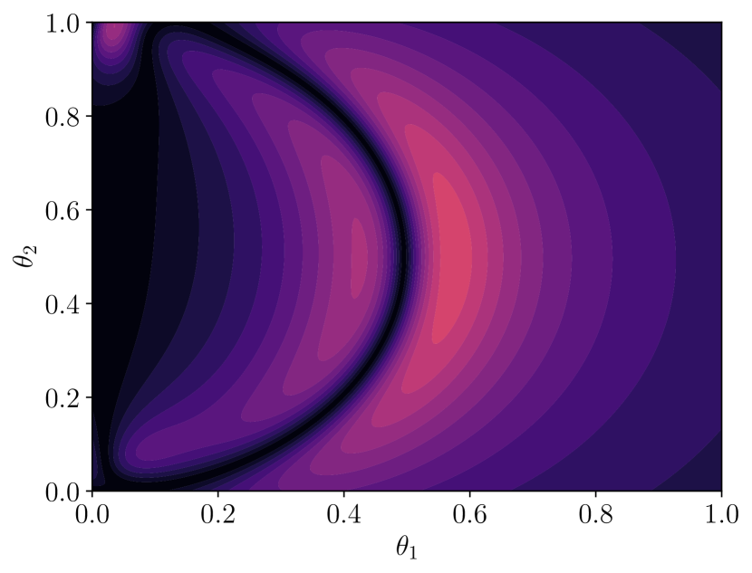
(a) $|\partial_{\theta_{1}}\Phi_{\rm KL}|$

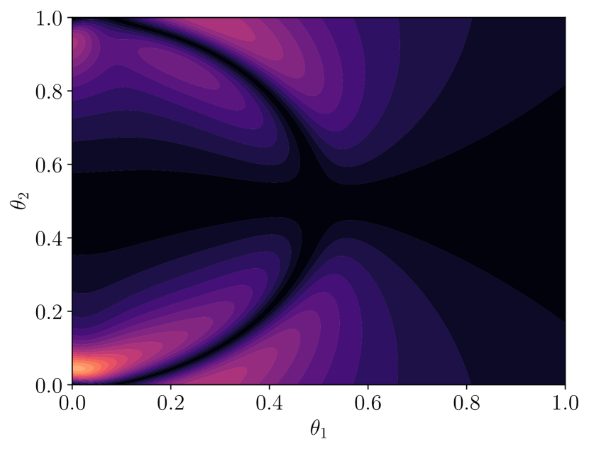
(b) $|\partial_{\theta_{2}}\Phi_{\rm KL}|$

Figure 1: Information gain sensitivities for two-dimensional model problem. Shown are the absolute values of the derivatives with respect to the auxiliary parameters.

The main target of this paper is to compute and understand derivatives of $D_{\rm KL}$ with respect to auxiliary parameters such as $\textstyle{\theta}$. In this example, these derivatives are straightforward to compute and their absolute values are shown in Figure 1 for $\mathbf{u}^{\text{obs}}=[0.15\;0.05]^{\top}$ and $\sigma=0.1$. Note that even for this simple example, the sensitivities exhibit complex behavior and change substantially for small changes in the auxiliary parameters. This is a common feature of sensitivity analysis in inverse problems.

The expression (4) for the information gain already hints towards challenges for infinite or high-dimensional parameters. For instance, the trace and determinant of the posterior covariance operator may be challenging to approximate, and $\mathbf{C}_{\rm post}$ and $\mathbf{m}_{\rm post}$ must be differentiated with respect to the auxiliary parameters $\textstyle{\theta}$. We will show how such a sensitivity analysis can be done for PDE-constrained linear inverse problems with infinite-dimensional parameters.

2 Preliminaries

In this section, we provide the background material for Bayesian linear inverse problems, adjoint-based gradient and Hessian computation, the information gain, and global sensitivity analysis.

2.1 Linear Bayesian Inverse Problems

Assume the forward model is governed by a PDE with its weak formulation represented abstractly as follows: the solution $u\in\mathcal{U}$ satisfies

$$\mathscr{A}(p,u;{\mathchoice{\mbox{\boldmath$\displaystyle{\theta}$}}{\mbox{\boldmath$\textstyle{\theta}$}}{\mbox{\boldmath$\scriptstyle{\theta}$}}{\mbox{\boldmath$\scriptscriptstyle{\theta}$}}})+\mathscr{C}(p,m;{\mathchoice{\mbox{\boldmath$\displaystyle{\theta}$}}{\mbox{\boldmath$\textstyle{\theta}$}}{\mbox{\boldmath$\scriptstyle{\theta}$}}{\mbox{\boldmath$\scriptscriptstyle{\theta}$}}})+\mathscr{D}(p;{\mathchoice{\mbox{\boldmath$\displaystyle{\theta}$}}{\mbox{\boldmath$\textstyle{\theta}$}}{\mbox{\boldmath$\scriptstyle{\theta}$}}{\mbox{\boldmath$\scriptscriptstyle{\theta}$}}})=0,\qquad\text{for all }p\in\mathcal{V}.$$ (5)

Here, $\mathcal{U}$ and $\mathcal{V}$ are appropriately chosen infinite-dimensional Hilbert spaces. The inversion parameter $m$ belongs to an infinite-dimensional Hilbert space $\mathcal{M}$. The set of the auxiliary parameters is denoted as $\Theta$. For simplicity, we assume this set is of the form $\Theta\vcentcolon=\Theta_{1}\times\dots\times\Theta_{{n_{\theta}}}$ with $\Theta_{i}\subset\mathbb{R}$ for each $i\in\{1,\ldots,{n_{\theta}}\}$. The form (5) is chosen to mimic a common type of weak form arising from linear PDEs that are linear in the inversion parameter and potentially contain non-homogeneous volume or boundary source terms. Therefore, we assume that all forms are linear in all inputs except for $\textstyle{\theta}$.

Typically, $\mathscr{A}$ represents a differential operator on the state variable, $\mathscr{C}$ is the term involving the inversion parameter, and $\mathscr{D}$ aggregates any miscellaneous boundary conditions or source terms that do not depend on the inversion parameters. As an example, consider the following elliptic PDE

$$-\Delta u+\theta u =m \Omega,$$    in (6)

$$\nabla u\cdot n =g \partial\Omega,$$    on

with the source term $m$ as the inversion parameter, and given boundary data $g$ and unit boundary normal $n$. This problem has the weak form (5) with

$$\mathscr{A}(p,u;\theta)=\int_{\Omega}\nabla u\cdot\nabla p+\theta up\differential{x},\quad\mathscr{C}(p,m)=\int_{\Omega}mp\differential{x}\quad\mathscr{D}(p)=\int_{\partial\Omega}gp\differential{s},$$ (7)

$\mathcal{U}=\mathcal{V}=H^{1}(\Omega)$, and $\mathcal{M}=L^{2}(\Omega)$. Note, the auxiliary parameter here only appears in $\mathscr{A}$, but in general it can appear in any of the forms.

Next, we consider a Bayesian inverse problem governed by (5). We assume that we have a vector of measurement data $\mathbf{u}^{\text{obs}}$ that relates to the inversion parameter $m$ via

$$\mathbf{u}^{\text{obs}}=\bm{\mathcal{F}}({\mathchoice{\mbox{\boldmath$\displaystyle{\theta}$}}{\mbox{\boldmath$\textstyle{\theta}$}}{\mbox{\boldmath$\scriptstyle{\theta}$}}{\mbox{\boldmath$\scriptscriptstyle{\theta}$}}})(m)+{\mathchoice{\mbox{\boldmath$\displaystyle{\eta}$}}{\mbox{\boldmath$\textstyle{\eta}$}}{\mbox{\boldmath$\scriptstyle{\eta}$}}{\mbox{\boldmath$\scriptscriptstyle{\eta}$}}}.$$ (8)

Here, $\bm{\mathcal{F}}$ is the parameter-to-observable map whose evaluation typically breaks down into two steps: solving (5) for $u$ and evaluating $u$ at the measurement points. The vector ${\mathchoice{\mbox{\boldmath$\displaystyle{\eta}$}}{\mbox{\boldmath$\textstyle{\eta}$}}{\mbox{\boldmath$\scriptstyle{\eta}$}}{\mbox{\boldmath$\scriptscriptstyle{\eta}$}}}\in\mathbb{R}^{N_{\text{obs}}}$ represents measurement error. We assume ${\mathchoice{\mbox{\boldmath$\displaystyle{\eta}$}}{\mbox{\boldmath$\textstyle{\eta}$}}{\mbox{\boldmath$\scriptstyle{\eta}$}}{\mbox{\boldmath$\scriptscriptstyle{\eta}$}}}\sim\mathcal{N}({\mathchoice{\mbox{\boldmath$\displaystyle{0}$}}{\mbox{\boldmath$\textstyle{0}$}}{\mbox{\boldmath$\scriptstyle{0}$}}{\mbox{\boldmath$\scriptscriptstyle{0}$}}},\mathbf{\Gamma}_{\text{noise}})$. Additionally, we assume $\mu_{\rm prior}=\mathcal{N}(m_{\text{prior}},\mathcal{C}_{\text{prior}})$. The specific choice of $\mathcal{C}_{\text{prior}}$ is important. This operator must be strictly positive, self-adjoint, and trace-class. A convenient approach for constructing such a $\mathcal{C}_{\text{prior}}$ is to define it as the inverse of Laplacian-like differential operator; see [28] for details. The prior measure induces the Cameron–Martin space $\mathcal{E}={\rm range}(\mathcal{C}_{\text{prior}}^{1/2})$ which is equipped with the inner product

$$\langle x,y\rangle_{\mathcal{C}_{\text{prior}}^{-1}}\vcentcolon=\langle\mathcal{C}_{\text{prior}}^{-1/2}x,\mathcal{C}_{\text{prior}}^{-1/2}y\rangle,\qquad\text{for all }x,y\in\mathcal{E}.$$ (9)

Finally, we further assume that $m_{\text{prior}}\in\mathcal{E}$.

With the data model and prior measure defined, Bayes’ formula in infinite dimensions [7] states that

$$\derivative{\mu_{\rm post}}{\mu_{\rm prior}}\propto\pi_{\rm like}(\mathbf{u}^{\text{obs}}|m;{\mathchoice{\mbox{\boldmath$\displaystyle{\theta}$}}{\mbox{\boldmath$\textstyle{\theta}$}}{\mbox{\boldmath$\scriptstyle{\theta}$}}{\mbox{\boldmath$\scriptscriptstyle{\theta}$}}}),$$ (10)

where $\pi_{\rm like}$ is the likelihood probability density function

$$\pi_{\rm like}(\mathbf{u}^{\text{obs}}|m;{\mathchoice{\mbox{\boldmath$\displaystyle{\theta}$}}{\mbox{\boldmath$\textstyle{\theta}$}}{\mbox{\boldmath$\scriptstyle{\theta}$}}{\mbox{\boldmath$\scriptscriptstyle{\theta}$}}})\propto\exp\left[-\frac{1}{2}\|\bm{\mathcal{F}}({\mathchoice{\mbox{\boldmath$\displaystyle{\theta}$}}{\mbox{\boldmath$\textstyle{\theta}$}}{\mbox{\boldmath$\scriptstyle{\theta}$}}{\mbox{\boldmath$\scriptscriptstyle{\theta}$}}})(m)-\mathbf{u}^{\text{obs}}\|_{\mathbf{\Gamma}_{\text{noise}}^{-1}}^{2}\right].$$ (11)

For a linear parameter-to-observable map, using Gaussian prior and noise models implies that the posterior measure is also Gaussian and has a simple closed form [28]. Note that in our abstract weak form (5), the presence of nonzero $\mathscr{D}$ makes $\bm{\mathcal{F}}$ affine as opposed to linear. This results in a Gaussian posterior with very similar closed form to the linear case, albeit with a slight change in the expression for the MAP point. This can, however, have a significant impact on the solution of the inverse problem. Henceforth, assuming an affine $\bm{\mathcal{F}}$, we write its action as

$$\bm{\mathcal{F}}(m)=\bm{\mathcal{G}}m+\bm{f}.$$ (12)

Here, $\bm{\mathcal{G}}\mathrel{\mathop{\ordinarycolon}}\mathcal{M}\to\mathbb{R}^{N_{\text{obs}}}$ is a continuous linear transformation and $\bm{f}\in\mathbb{R}^{N_{\text{obs}}}$. The resulting closed form expressions for the mean and covariance of the Gaussian posterior are [28]

$$\mu_{\rm post}=\mathcal{N}(m_{{\text{post}}},\mathcal{C}_{\text{post}}),\quad\text{where}\quad\begin{cases}\mathcal{C}_{\text{post}}=(\bm{\mathcal{G}}^{*}\mathbf{\Gamma}_{\text{noise}}^{-1}\bm{\mathcal{G}}+\mathcal{C}_{\text{prior}}^{-1})^{-1},\\ m_{{\text{post}}}=\mathcal{C}_{\text{post}}\left[\bm{\mathcal{G}}^{*}\mathbf{\Gamma}_{\text{noise}}^{-1}(\mathbf{u}^{\text{obs}}-\bm{f})+\mathcal{C}_{\text{prior}}^{-1}m_{\text{prior}}\right].\end{cases}$$ (13)

2.2 Adjoint-Based Gradient and Hessian Computation

Generally, the MAP point $m_{{\text{post}}}$ can be obtained by minimizing

$$\mathcal{J}(m;{\mathchoice{\mbox{\boldmath$\displaystyle{\theta}$}}{\mbox{\boldmath$\textstyle{\theta}$}}{\mbox{\boldmath$\scriptstyle{\theta}$}}{\mbox{\boldmath$\scriptscriptstyle{\theta}$}}})\vcentcolon=\frac{1}{2}\|\bm{\mathcal{F}}({\mathchoice{\mbox{\boldmath$\displaystyle{\theta}$}}{\mbox{\boldmath$\textstyle{\theta}$}}{\mbox{\boldmath$\scriptstyle{\theta}$}}{\mbox{\boldmath$\scriptscriptstyle{\theta}$}}})(m)-\mathbf{u}^{\text{obs}}\|_{\mathbf{\Gamma}_{\text{noise}}^{-1}}^{2}+\frac{1}{2}\|m-m_{\text{prior}}\|_{\mathcal{C}_{\text{prior}}^{-1}}^{2},$$ (14)

over $\mathcal{E}$. In the linear Gaussian settings, this is a “regularized” linear least squares problem. In what follows, we need the adjoint-based expressions [15, 24, 12] for the gradient and Hessian of $\mathcal{J}$ with respect to $m$. These expressions and the approach for their derivation are central to our proposed methods. Assume that (5) has a unique solution $u(m;{\mathchoice{\mbox{\boldmath$\displaystyle{\theta}$}}{\mbox{\boldmath$\textstyle{\theta}$}}{\mbox{\boldmath$\scriptstyle{\theta}$}}{\mbox{\boldmath$\scriptscriptstyle{\theta}$}}})$ for every $m\in\mathcal{M}$ and ${\mathchoice{\mbox{\boldmath$\displaystyle{\theta}$}}{\mbox{\boldmath$\textstyle{\theta}$}}{\mbox{\boldmath$\scriptstyle{\theta}$}}{\mbox{\boldmath$\scriptscriptstyle{\theta}$}}}\in\Theta$. Next, we define a linear observation operator $\bm{\mathcal{Q}}\mathrel{\mathop{\ordinarycolon}}\mathcal{V}\to\mathbb{R}^{N_{\text{obs}}}$, which extracts solution values at the measurement points. Thus, we can write $\bm{\mathcal{F}}({\mathchoice{\mbox{\boldmath$\displaystyle{\theta}$}}{\mbox{\boldmath$\textstyle{\theta}$}}{\mbox{\boldmath$\scriptstyle{\theta}$}}{\mbox{\boldmath$\scriptscriptstyle{\theta}$}}})(m)=\bm{\mathcal{Q}}u(m;{\mathchoice{\mbox{\boldmath$\displaystyle{\theta}$}}{\mbox{\boldmath$\textstyle{\theta}$}}{\mbox{\boldmath$\scriptstyle{\theta}$}}{\mbox{\boldmath$\scriptscriptstyle{\theta}$}}})$.

To facilitate derivative computation, we follow a formal Lagrange approach. To this end, we consider the Lagrangian

$$\mathcal{L}(u,p,m)\vcentcolon=\frac{1}{2}\|\bm{\mathcal{Q}}u-\mathbf{u}^{\text{obs}}\|_{\mathbf{\Gamma}_{\text{noise}}^{-1}}^{2}+\frac{1}{2}\|m-m_{\text{prior}}\|_{\mathcal{C}_{\text{prior}}^{-1}}^{2}+\mathscr{A}(p,u;{\mathchoice{\mbox{\boldmath$\displaystyle{\theta}$}}{\mbox{\boldmath$\textstyle{\theta}$}}{\mbox{\boldmath$\scriptstyle{\theta}$}}{\mbox{\boldmath$\scriptscriptstyle{\theta}$}}})+\mathscr{C}(p,m;{\mathchoice{\mbox{\boldmath$\displaystyle{\theta}$}}{\mbox{\boldmath$\textstyle{\theta}$}}{\mbox{\boldmath$\scriptstyle{\theta}$}}{\mbox{\boldmath$\scriptscriptstyle{\theta}$}}})+\mathscr{D}(p;{\mathchoice{\mbox{\boldmath$\displaystyle{\theta}$}}{\mbox{\boldmath$\textstyle{\theta}$}}{\mbox{\boldmath$\scriptstyle{\theta}$}}{\mbox{\boldmath$\scriptscriptstyle{\theta}$}}}).$$ (15)

The gradient of $\mathcal{J}$ at $m$ in direction $\tilde{m}$, denoted by $\mathcal{G}(m)(\tilde{m})$, is given by

$$\mathcal{G}(m)(\tilde{m})\vcentcolon=\mathcal{L}_{m}(u,p,m)(\tilde{m}),$$

where $u$ and $p$, respectively, satisfy the state and adjoint equations:

$$\mathcal{L}_{p}(u,p,m)(\tilde{p}) =0,\quad\forall\tilde{p}\in\mathcal{V},$$

$$\mathcal{L}_{u}(u,p,m)(\tilde{u}) =0,\quad\forall\tilde{u}\in\mathcal{V}.$$

For the class of inverse problems under study, these expressions take the form

$$\mathcal{G}(m)(\tilde{m})=\langle m-m_{\text{prior}},\tilde{m}\rangle_{\mathcal{C}_{\text{prior}}^{-1}}+\mathscr{C}(p,\tilde{m};{\mathchoice{\mbox{\boldmath$\displaystyle{\theta}$}}{\mbox{\boldmath$\textstyle{\theta}$}}{\mbox{\boldmath$\scriptstyle{\theta}$}}{\mbox{\boldmath$\scriptscriptstyle{\theta}$}}}),$$ (16)

where

$$\mathscr{A}(\tilde{p},u;{\mathchoice{\mbox{\boldmath$\displaystyle{\theta}$}}{\mbox{\boldmath$\textstyle{\theta}$}}{\mbox{\boldmath$\scriptstyle{\theta}$}}{\mbox{\boldmath$\scriptscriptstyle{\theta}$}}})+\mathscr{C}(\tilde{p},m;{\mathchoice{\mbox{\boldmath$\displaystyle{\theta}$}}{\mbox{\boldmath$\textstyle{\theta}$}}{\mbox{\boldmath$\scriptstyle{\theta}$}}{\mbox{\boldmath$\scriptscriptstyle{\theta}$}}})+\mathscr{D}(\tilde{p};{\mathchoice{\mbox{\boldmath$\displaystyle{\theta}$}}{\mbox{\boldmath$\textstyle{\theta}$}}{\mbox{\boldmath$\scriptstyle{\theta}$}}{\mbox{\boldmath$\scriptscriptstyle{\theta}$}}})=0, \quad\forall\tilde{p}\in\mathcal{V},$$

$$\langle\bm{\mathcal{Q}}u-\mathbf{u}^{\text{obs}},\bm{\mathcal{Q}}\tilde{u}\rangle_{\mathbf{\Gamma}_{\text{noise}}^{-1}}+\mathscr{A}(\tilde{u},p;{\mathchoice{\mbox{\boldmath$\displaystyle{\theta}$}}{\mbox{\boldmath$\textstyle{\theta}$}}{\mbox{\boldmath$\scriptstyle{\theta}$}}{\mbox{\boldmath$\scriptscriptstyle{\theta}$}}})=0, \quad\forall\tilde{u}\in\mathcal{V}.$$

Likewise, we can define the Hessian of (14) by considering the meta-Lagrangian [12]:

$$\mathcal{L}^{H}(u,p,m,\hat{u},\hat{p},\hat{m})\vcentcolon=\mathcal{L}_{m}(\hat{m})+\mathcal{L}_{u}(\hat{u})+\mathcal{L}_{p}(\hat{p}).$$ (17)

Note that, for notational convenience, we have suppressed the dependence of $\mathcal{L}$ on $(u,p,m)$. The Hessian action $\mathcal{H}(\hat{m},\tilde{m})$ is given by $\mathcal{H}(\hat{m},\tilde{m})\vcentcolon=\mathcal{L}^{H}_{m}(u,p,m,\hat{u},\hat{p},\hat{m})(\tilde{m})$, where $\hat{u}$ and $\hat{p}$ are obtained, respectively, by setting the variations of $\mathcal{L}^{H}$ with respect to $p$ and $u$ to zero. For the case of linear inverse problems under study,

$$\mathcal{H}(\hat{m},\tilde{m})=\langle\tilde{m},\hat{m}\rangle_{\mathcal{C}_{\text{prior}}^{-1}}+\mathscr{C}(\hat{p},\tilde{m};{\mathchoice{\mbox{\boldmath$\displaystyle{\theta}$}}{\mbox{\boldmath$\textstyle{\theta}$}}{\mbox{\boldmath$\scriptstyle{\theta}$}}{\mbox{\boldmath$\scriptscriptstyle{\theta}$}}}),$$ (18a)

where

$$\mathscr{A}(\tilde{p},\hat{u};{\mathchoice{\mbox{\boldmath$\displaystyle{\theta}$}}{\mbox{\boldmath$\textstyle{\theta}$}}{\mbox{\boldmath$\scriptstyle{\theta}$}}{\mbox{\boldmath$\scriptscriptstyle{\theta}$}}})+\mathscr{C}(\tilde{p},\hat{m};{\mathchoice{\mbox{\boldmath$\displaystyle{\theta}$}}{\mbox{\boldmath$\textstyle{\theta}$}}{\mbox{\boldmath$\scriptstyle{\theta}$}}{\mbox{\boldmath$\scriptscriptstyle{\theta}$}}})=0,\quad\forall\tilde{p}\in\mathcal{V},$$ (18b)

$$\langle\bm{\mathcal{Q}}\tilde{u},\bm{\mathcal{Q}}\hat{u}\rangle_{\mathbf{\Gamma}_{\text{noise}}^{-1}}+\mathscr{A}(\hat{p},\tilde{u};{\mathchoice{\mbox{\boldmath$\displaystyle{\theta}$}}{\mbox{\boldmath$\textstyle{\theta}$}}{\mbox{\boldmath$\scriptstyle{\theta}$}}{\mbox{\boldmath$\scriptscriptstyle{\theta}$}}})=0,\quad\forall\tilde{u}\in\mathcal{V}.$$ (18c)

Note that, since we focus on linear/affine inverse problems, the Hessian has no dependency on the inversion parameter $m$. The equations (18b) and (18c) are the so-called incremental state and incremental adjoint equations. Of additional interest is the Hessian of only the data misfit term in (14), denoted as the data-misfit Hessian $\mathcal{H}_{\rm misfit}$. Following a similar procedure to the above, we have

$$\mathcal{H}_{\rm misfit}(\hat{m},\tilde{m})=\mathscr{C}(\hat{p},\tilde{m};{\mathchoice{\mbox{\boldmath$\displaystyle{\theta}$}}{\mbox{\boldmath$\textstyle{\theta}$}}{\mbox{\boldmath$\scriptstyle{\theta}$}}{\mbox{\boldmath$\scriptscriptstyle{\theta}$}}}),$$ (19)

where

$$\mathscr{A}(\tilde{p},\hat{u};{\mathchoice{\mbox{\boldmath$\displaystyle{\theta}$}}{\mbox{\boldmath$\textstyle{\theta}$}}{\mbox{\boldmath$\scriptstyle{\theta}$}}{\mbox{\boldmath$\scriptscriptstyle{\theta}$}}})+\mathscr{C}(\tilde{p},\hat{m};{\mathchoice{\mbox{\boldmath$\displaystyle{\theta}$}}{\mbox{\boldmath$\textstyle{\theta}$}}{\mbox{\boldmath$\scriptstyle{\theta}$}}{\mbox{\boldmath$\scriptscriptstyle{\theta}$}}})=0, \quad\forall\tilde{p}\in\mathcal{V},$$

$$\langle\bm{\mathcal{Q}}\tilde{u},\bm{\mathcal{Q}}\hat{u}\rangle_{\mathbf{\Gamma}_{\text{noise}}^{-1}}+\mathscr{A}(\hat{p},\tilde{u};{\mathchoice{\mbox{\boldmath$\displaystyle{\theta}$}}{\mbox{\boldmath$\textstyle{\theta}$}}{\mbox{\boldmath$\scriptstyle{\theta}$}}{\mbox{\boldmath$\scriptscriptstyle{\theta}$}}})=0, \quad\forall\tilde{u}\in\mathcal{V}.$$

2.3 Quantities of Interest for Bayesian Inference: The Information Gain

To perform sensitivity analysis on the posterior distribution of an inverse problem, we consider scalar quantities of interest (QoIs) that describe specific aspects of the posterior measure. As mentioned in the introduction, one possibility is to consider optimal experimental design (OED) criteria, which provide different measures of uncertainty in the parameters. A classical approach to deriving Bayesian OED criteria is to adapt ideas from information theory. In that context, a natural metric for individual distributions is (Shannon) entropy. However, the continuous analogue of entropy, the differential entropy, lacks many fundamental properties of its discrete counterpart. Instead, it is common to use the relative entropy, as given by the Kullback–Leibler (KL) divergence from the posterior to the prior:

$$D_{\rm KL}(\mu_{\rm post}||\mu_{\rm prior})\vcentcolon=\int_{\mathcal{M}}\log\left[\derivative{\mu_{\rm post}}{\mu_{\rm prior}}\right]\differential{\mu_{\rm post}}.$$

The notion of relative entropy has seen much recent popularity in the machine learning literature, notably for variational auto-encoders [17] and information bottlenecks [31]. In Bayesian analysis, the relative entropy provides a measure of information gain. In that context, the expected relative entropy, also known as the expected information gain, is a classical choice for a design criterion. This is also known as the Bayesian D-optimality criterion. This expected information gain is defined as the expectation of the KL-divergence over data:

$$\overline{D_{\rm KL}}(\mu_{\rm post}||\mu_{\rm prior})\vcentcolon=\operatorname{\mathbb{E}}_{\mathbf{u}^{\text{obs}}}\left[D_{\rm KL}(\mu_{\rm post}||\mu_{\rm prior})\right].$$ (20)

For linear Gaussian inverse problems, the information gain has a closed-form expression. Furthermore, it has been shown that a similar analytic expression can be derived in the infinite-dimensional setting [2]:

$$D_{\rm KL}(\mu_{\rm post}||\mu_{\rm prior})\vcentcolon=\frac{1}{2}\left[\log\det(\tilde{\mathcal{H}}_{\rm misfit}+I)-\hbox{Tr}(\mathcal{H}_{\rm misfit}\mathcal{C}_{\text{post}})+\langle m_{{\text{post}}}-m_{\text{prior}},m_{{\text{post}}}-m_{\text{prior}}\rangle_{\mathcal{C}_{\text{prior}}^{-1}}\right],$$ (21)

where $\tilde{\mathcal{H}}_{\rm misfit}$ is the prior-preconditioned data-misfit Hessian, given by

$$\tilde{\mathcal{H}}_{\rm misfit}\vcentcolon=\mathcal{C}_{\text{prior}}^{1/2}\mathcal{H}_{\rm misfit}\mathcal{C}_{\text{prior}}^{1/2}.$$ (22)

We seek to assess the (derivative-based) sensitivity of quantities such as the information gain to the auxiliary parameters in the governing PDEs. As before, we let $\textstyle{\theta}$ denote a vector of auxiliary parameters. In this setting, the posterior measure depends on $\textstyle{\theta}$ as well. In what follows, we denote $\Phi_{\rm KL}({\mathchoice{\mbox{\boldmath$\displaystyle{\theta}$}}{\mbox{\boldmath$\textstyle{\theta}$}}{\mbox{\boldmath$\scriptstyle{\theta}$}}{\mbox{\boldmath$\scriptscriptstyle{\theta}$}}})\vcentcolon=D_{\rm KL}(\mu_{\rm post}({\mathchoice{\mbox{\boldmath$\displaystyle{\theta}$}}{\mbox{\boldmath$\textstyle{\theta}$}}{\mbox{\boldmath$\scriptstyle{\theta}$}}{\mbox{\boldmath$\scriptscriptstyle{\theta}$}}})||\mu_{\rm prior})$. Likewise, we write the expected information gain as $\overline{\Phi}_{\rm KL}({\mathchoice{\mbox{\boldmath$\displaystyle{\theta}$}}{\mbox{\boldmath$\textstyle{\theta}$}}{\mbox{\boldmath$\scriptstyle{\theta}$}}{\mbox{\boldmath$\scriptscriptstyle{\theta}$}}})\vcentcolon=\overline{D_{\rm KL}}(\mu_{\rm post}({\mathchoice{\mbox{\boldmath$\displaystyle{\theta}$}}{\mbox{\boldmath$\textstyle{\theta}$}}{\mbox{\boldmath$\scriptstyle{\theta}$}}{\mbox{\boldmath$\scriptscriptstyle{\theta}$}}})||\mu_{\rm prior})$. Note that for linear Gaussian inverse problems,

$$\overline{\Phi}_{\rm KL}({\mathchoice{\mbox{\boldmath$\displaystyle{\theta}$}}{\mbox{\boldmath$\textstyle{\theta}$}}{\mbox{\boldmath$\scriptstyle{\theta}$}}{\mbox{\boldmath$\scriptscriptstyle{\theta}$}}})=\frac{1}{2}\log\det(\tilde{\mathcal{H}}_{\rm misfit}+I).$$

2.4 Global Sensitivity via Derivative-Based Upper Bounds for Sobol Indices

A standard derivative-based sensitivity analysis of the information gain provides only local sensitivity information. It is also of interest to perform global sensitivity analysis. A standard approach in the uncertainty quantification literature is to use a variance-based global sensitivity analysis approach. This involves computing variance-based indices known as Sobol indices [25, 26]. Computing such indices requires an expensive sampling procedure, which would be computationally challenging for the quantities of interests considered in the present work. This is due to the need for a potentially large number of QoI evaluations. Instead, we rely on derivative-based upper bounds for total Sobol indices [27, 19], which provide a tractable approach for global sensitivity analysis of the information gain.

We assume that the entries of ${\mathchoice{\mbox{\boldmath$\displaystyle{\theta}$}}{\mbox{\boldmath$\textstyle{\theta}$}}{\mbox{\boldmath$\scriptstyle{\theta}$}}{\mbox{\boldmath$\scriptscriptstyle{\theta}$}}}\in\Theta$ are independent random variables with cumulative density functions (CDFs) $F_{1},\dots,F_{n_{\theta}}$. Also, we assume $\Phi_{\rm KL}\in L^{2}(\Theta,\sigma({\mathchoice{\mbox{\boldmath$\displaystyle{\theta}$}}{\mbox{\boldmath$\textstyle{\theta}$}}{\mbox{\boldmath$\scriptstyle{\theta}$}}{\mbox{\boldmath$\scriptscriptstyle{\theta}$}}}),F)$, where $\sigma({\mathchoice{\mbox{\boldmath$\displaystyle{\theta}$}}{\mbox{\boldmath$\textstyle{\theta}$}}{\mbox{\boldmath$\scriptstyle{\theta}$}}{\mbox{\boldmath$\scriptscriptstyle{\theta}$}}})$ is the $\sigma$-algebra generated by $\{\theta_{i}\}_{i=1}^{n_{\theta}}$, and $F$ is the joint CDF of $\textstyle{\theta}$. The first order Sobol indices are given by

$$S_{i}\vcentcolon=\frac{\operatorname{Var}[\operatorname{\mathbb{E}}[\Phi_{\rm KL}({\mathchoice{\mbox{\boldmath$\displaystyle{\theta}$}}{\mbox{\boldmath$\textstyle{\theta}$}}{\mbox{\boldmath$\scriptstyle{\theta}$}}{\mbox{\boldmath$\scriptscriptstyle{\theta}$}}})|\theta_{i}]]}{\operatorname{Var}[\Phi_{\rm KL}({\mathchoice{\mbox{\boldmath$\displaystyle{\theta}$}}{\mbox{\boldmath$\textstyle{\theta}$}}{\mbox{\boldmath$\scriptstyle{\theta}$}}{\mbox{\boldmath$\scriptscriptstyle{\theta}$}}})]},\;i=1,\dots,n_{\theta}.$$ (23)

Here, $S_{i}$ can be interpreted as quantifying the contribution of $\theta_{i}$ on $\operatorname{Var}[\Phi_{\rm KL}({\mathchoice{\mbox{\boldmath$\displaystyle{\theta}$}}{\mbox{\boldmath$\textstyle{\theta}$}}{\mbox{\boldmath$\scriptstyle{\theta}$}}{\mbox{\boldmath$\scriptscriptstyle{\theta}$}}})]$. One can also define higher order sensitivity indices that, in addition to first order effects, account for interactions between random inputs. To this end, we consider the total Sobol indices

$$S^{\mathrm{tot}}_{i}\vcentcolon=\frac{\operatorname{\mathbb{E}}[\operatorname{Var}[\Phi_{\rm KL}({\mathchoice{\mbox{\boldmath$\displaystyle{\theta}$}}{\mbox{\boldmath$\textstyle{\theta}$}}{\mbox{\boldmath$\scriptstyle{\theta}$}}{\mbox{\boldmath$\scriptscriptstyle{\theta}$}}})|{\mathchoice{\mbox{\boldmath$\displaystyle{\theta}$}}{\mbox{\boldmath$\textstyle{\theta}$}}{\mbox{\boldmath$\scriptstyle{\theta}$}}{\mbox{\boldmath$\scriptscriptstyle{\theta}$}}}^{\sim i}]]}{\operatorname{Var}[\Phi_{\rm KL}({\mathchoice{\mbox{\boldmath$\displaystyle{\theta}$}}{\mbox{\boldmath$\textstyle{\theta}$}}{\mbox{\boldmath$\scriptstyle{\theta}$}}{\mbox{\boldmath$\scriptscriptstyle{\theta}$}}})]}=\frac{\operatorname{Var}[\Phi_{\rm KL}({\mathchoice{\mbox{\boldmath$\displaystyle{\theta}$}}{\mbox{\boldmath$\textstyle{\theta}$}}{\mbox{\boldmath$\scriptstyle{\theta}$}}{\mbox{\boldmath$\scriptscriptstyle{\theta}$}}})]-\operatorname{Var}[\operatorname{\mathbb{E}}[\Phi_{\rm KL}({\mathchoice{\mbox{\boldmath$\displaystyle{\theta}$}}{\mbox{\boldmath$\textstyle{\theta}$}}{\mbox{\boldmath$\scriptstyle{\theta}$}}{\mbox{\boldmath$\scriptscriptstyle{\theta}$}}})|{\mathchoice{\mbox{\boldmath$\displaystyle{\theta}$}}{\mbox{\boldmath$\textstyle{\theta}$}}{\mbox{\boldmath$\scriptstyle{\theta}$}}{\mbox{\boldmath$\scriptscriptstyle{\theta}$}}}^{\sim i}]]}{\operatorname{Var}[\Phi_{\rm KL}({\mathchoice{\mbox{\boldmath$\displaystyle{\theta}$}}{\mbox{\boldmath$\textstyle{\theta}$}}{\mbox{\boldmath$\scriptstyle{\theta}$}}{\mbox{\boldmath$\scriptscriptstyle{\theta}$}}})]},$$ (24)

where

$${\mathchoice{\mbox{\boldmath$\displaystyle{\theta}$}}{\mbox{\boldmath$\textstyle{\theta}$}}{\mbox{\boldmath$\scriptstyle{\theta}$}}{\mbox{\boldmath$\scriptscriptstyle{\theta}$}}}^{\sim i}\vcentcolon=[\theta_{1}\;\cdots\;\theta_{i-1}\;\theta_{i+1}\;\cdots,\theta_{n_{\theta}}]^{\top}\in\mathbb{R}^{n_{\theta}-1}.$$ (25)

Note that $S^{\mathrm{tot}}_{i}$ quantifies the contribution of $\theta_{i}$ by itself, and through its interactions with the other entries of $\textstyle{\theta}$, to $\operatorname{Var}[\Phi_{\rm KL}({\mathchoice{\mbox{\boldmath$\displaystyle{\theta}$}}{\mbox{\boldmath$\textstyle{\theta}$}}{\mbox{\boldmath$\scriptstyle{\theta}$}}{\mbox{\boldmath$\scriptscriptstyle{\theta}$}}})]$.

It has been shown in [19], utilizing the $L^{2}$-Poincaré inequality

$$\int\Phi_{\rm KL}({\mathchoice{\mbox{\boldmath$\displaystyle{\theta}$}}{\mbox{\boldmath$\textstyle{\theta}$}}{\mbox{\boldmath$\scriptstyle{\theta}$}}{\mbox{\boldmath$\scriptscriptstyle{\theta}$}}})^{2}\differential{F({\mathchoice{\mbox{\boldmath$\displaystyle{\theta}$}}{\mbox{\boldmath$\textstyle{\theta}$}}{\mbox{\boldmath$\scriptstyle{\theta}$}}{\mbox{\boldmath$\scriptscriptstyle{\theta}$}}})}\leq C(F)\int\|\nabla\Phi_{\rm KL}({\mathchoice{\mbox{\boldmath$\displaystyle{\theta}$}}{\mbox{\boldmath$\textstyle{\theta}$}}{\mbox{\boldmath$\scriptstyle{\theta}$}}{\mbox{\boldmath$\scriptscriptstyle{\theta}$}}})\|^{2}\differential{F({\mathchoice{\mbox{\boldmath$\displaystyle{\theta}$}}{\mbox{\boldmath$\textstyle{\theta}$}}{\mbox{\boldmath$\scriptstyle{\theta}$}}{\mbox{\boldmath$\scriptscriptstyle{\theta}$}}})},$$ (26)

that these total sensitivity indices obey the upper bound

$$S^{\mathrm{tot}}_{i}\leq\frac{C(F_{i})}{\operatorname{Var}[\Phi_{\rm KL}({\mathchoice{\mbox{\boldmath$\displaystyle{\theta}$}}{\mbox{\boldmath$\textstyle{\theta}$}}{\mbox{\boldmath$\scriptstyle{\theta}$}}{\mbox{\boldmath$\scriptscriptstyle{\theta}$}}})]}\int\left(\partialderivative{\theta_{i}}\Phi_{\rm KL}({\mathchoice{\mbox{\boldmath$\displaystyle{\theta}$}}{\mbox{\boldmath$\textstyle{\theta}$}}{\mbox{\boldmath$\scriptstyle{\theta}$}}{\mbox{\boldmath$\scriptscriptstyle{\theta}$}}})\right)^{2}\differential{F({\mathchoice{\mbox{\boldmath$\displaystyle{\theta}$}}{\mbox{\boldmath$\textstyle{\theta}$}}{\mbox{\boldmath$\scriptstyle{\theta}$}}{\mbox{\boldmath$\scriptscriptstyle{\theta}$}}})}.$$ (27)

Here, $C(F_{i})$ is the Poincare constant corresponding to CDF $F_{i}$. For example, if $\theta_{i}$ is uniformly distributed random variable on $[-1,1]$, the corresponding Poincaré constant is $C(F_{i})=4/\pi^{2}$; see [27, 19].

The above discussion shows that an efficient computational approach for computing derivatives of the information gain at arbitrary choices of $\textstyle{\theta}$ enables the approximation of an upper bound for the total order Sobol indices. This provides global sensitivity measures that take the ranges of uncertainty in the auxiliary parameters into account.

3 Method

In this section, we outline a scalable computational approach for sensitivity analysis of (21) with respect to the auxiliary parameters. Our approach combines low-rank spectral decompositions (see Section 3.1) and adjoint-based eigenvalue sensitivity analysis (see Section 3.2). We also need to borrow tools from post-optimal sensitivity analysis to compute the derivative of the term involving the MAP point, in the definition of (21). This is outlined in Section 3.3. In Section 3.4, we summarize the overall computational procedure for sensitivity analysis of the information gain, and discuss the computational cost of the proposed approach, in terms of the required number of PDE solves.

3.1 Low-Rank Approximation of the Information Gain

Consider the data-misfit Hessian described implicitly in (19), which has the following closed form for affine inverse problems under study

$$\mathcal{H}_{\rm misfit}\vcentcolon=\bm{\mathcal{G}}^{*}\mathbf{\Gamma}_{\text{noise}}^{-1}\bm{\mathcal{G}},$$ (28)

where $\bm{\mathcal{G}}$ is as in (12). This is a positive self-adjoint trace-class operator, and thus has a spectral decomposition with non-negative eigenvalues and orthonormal eigenvectors. Recall also that the observations are finite-dimensional and belong to $\mathbb{R}^{N_{\text{obs}}}$. Thus, the range of $\mathcal{H}_{\rm misfit}$ has finite dimension $N_{\text{obs}}$. Moreover, in inverse problems governed by PDEs with smoothing forward operators the eigenvalues of this Hessian operator decay rapidly and the numerical rank of $\mathcal{H}_{\rm misfit}$ is typically smaller than $N_{\text{obs}}$. In what follows, we need the prior-preconditioned data misfit Hessian, $\tilde{\mathcal{H}}_{\rm misfit}$, defined in (22). This prior-preconditioned operator typically exhibits faster spectral decay than $\mathcal{H}_{\rm misfit}$ [5]. This low-rank structure can be used to construct efficient approximations to the posterior covariance operator [7]. Here, we use this problem structure to efficiently approximate the information gain.

Consider a low-rank approximation of $\tilde{\mathcal{H}}_{\rm misfit}$:

$$\tilde{\mathcal{H}}_{\rm misfit}\phi=\sum_{n=1}^{\infty}\gamma_{n}\langle\phi,\omega_{n}\rangle\omega_{n}\approx\sum_{n=1}^{r}\gamma_{n}\langle\phi,\omega_{n}\rangle\omega_{n},$$ (29)

where $\phi$ is any function in $\mathcal{M}$ and $r\leq N_{\text{obs}}$ is some appropriately chosen constant such that $(\gamma_{n},\omega_{n})$ are the dominant eigenpairs of $\tilde{\mathcal{H}}_{\rm misfit}$ given by the eigenvalue problem

$$\tilde{\mathcal{H}}_{\rm misfit}(\omega_{i},\phi)=\gamma_{i}\langle\phi,\omega_{i}\rangle,\quad\text{with}\quad\langle\omega_{i},\omega_{i}\rangle=1,\qquad\forall\phi\in\mathcal{M},i\in\{1,\dots,r\}.$$ (30)

We assume that the dominant eigenvalues are not repeated, which is typically the case due to their rapid decay in inverse problems under study. This assumption is sufficient to ensure the regularity of the eigenvalue problem, see [21]. Using the low-rank approximation (29), we approximate the information gain as follows:

$$\Phi_{\rm KL}\approx\hat{\Phi}_{\rm KL}\vcentcolon=\frac{1}{2}\left[\sum_{i=1}^{r}\log(1+\gamma_{i})-\sum_{i=1}^{r}\frac{\gamma_{i}}{1+\gamma_{i}}+\|m_{{\text{post}}}-m_{\text{prior}}\|_{\mathcal{C}_{\text{prior}}^{-1}}^{2}\right].$$ (31)

This will be our surrogate for the purposes of sensitivity analysis. Note that the (low-rank) spectral decomposition of the prior-preconditioned data misfit Hessian is typically computed in the process of Bayesian analysis in linear(ized) inverse problems. In such cases, without any additional effort, we have at hand a fast method for evaluating the information gain. Such low-rank approximations to the information gain were also considered, in a discretized setting in [5]. Here, we utilize this approximation, in an infinite-dimensional setting, to derive efficient adjoint-based expressions for the eigenvalue derivatives using which we can efficiently compute the derivatives of the information gain with respect to auxiliary parameters.

3.2 Adjoint-Based Eigenvalue Sensitivity

Since the eigenvalues are only involved in the first two terms of (31), we first focus on this part for sensitivity analysis and consider the function

$$\Phi_{\rm KL}^{\gamma}\vcentcolon=\frac{1}{2}\sum_{i=1}^{r}\left[\log(1+\gamma_{i})-\frac{\gamma_{i}}{1+\gamma_{i}}\right].$$ (32)

This has a dependency on $\textstyle{\theta}$ through the eigenvalues of the prior-preconditioned data misfit Hessian $\tilde{\mathcal{H}}_{\rm misfit}$. Hence, the question of computing $\partial_{\theta_{j}}\Phi_{\rm KL}^{\gamma}$ comes down to computing $\partial_{\theta_{j}}\gamma_{i}$, for $j\in\{1,\ldots,r\}$. To take advantage of the existing adjoint-based expressions for the data-misfit Hessian, we transform the eigenvalue problem (30) to the generalized eigenvalue problem

$$\mathcal{H}_{\rm misfit}(\psi_{i},\phi)=\gamma_{i}\langle\phi,\psi_{i}\rangle_{\mathcal{C}_{\text{prior}}^{-1}}\quad\text{and}\quad\langle\psi_{i},\psi_{i}\rangle_{\mathcal{C}_{\text{prior}}^{-1}}=1,\qquad\forall\phi\in\mathcal{M},\forall i\in\{1,\dots,r\},$$ (33)

where $\psi_{i}=\mathcal{C}_{\text{prior}}^{1/2}\omega_{i}$. Since evaluating (32) only requires eigenvalues which remain unchanged in (33), it is equivalent to use this new eigenvalue problem. Now, leveraging (19) which implicitly defines the action of $\mathcal{H}_{\rm misfit}$, we can write the full system constraining the evaluation of (32) as

$$\Phi_{\rm KL}^{\gamma}=\frac{1}{2}\sum_{i=1}^{r}\left[\log(1+\mathscr{C}(\hat{p}_{i},\psi_{i};{\mathchoice{\mbox{\boldmath$\displaystyle{\theta}$}}{\mbox{\boldmath$\textstyle{\theta}$}}{\mbox{\boldmath$\scriptstyle{\theta}$}}{\mbox{\boldmath$\scriptscriptstyle{\theta}$}}}))-\frac{\mathscr{C}(\hat{p}_{i},\psi_{i};{\mathchoice{\mbox{\boldmath$\displaystyle{\theta}$}}{\mbox{\boldmath$\textstyle{\theta}$}}{\mbox{\boldmath$\scriptstyle{\theta}$}}{\mbox{\boldmath$\scriptscriptstyle{\theta}$}}})}{1+\mathscr{C}(\hat{p}_{i},\psi_{i};{\mathchoice{\mbox{\boldmath$\displaystyle{\theta}$}}{\mbox{\boldmath$\textstyle{\theta}$}}{\mbox{\boldmath$\scriptstyle{\theta}$}}{\mbox{\boldmath$\scriptscriptstyle{\theta}$}}})}\right],$$ (34a)

where for $$i\in\{1,\dots,r\}$$,

$$\begin{cases}\langle\bm{\mathcal{Q}}\tilde{u},\bm{\mathcal{Q}}\hat{u}_{i}\rangle_{\mathbf{\Gamma}_{\text{noise}}^{-1}}+\mathscr{A}(\hat{p}_{i},\tilde{u};{\mathchoice{\mbox{\boldmath$\displaystyle{\theta}$}}{\mbox{\boldmath$\textstyle{\theta}$}}{\mbox{\boldmath$\scriptstyle{\theta}$}}{\mbox{\boldmath$\scriptscriptstyle{\theta}$}}})=0,&\forall\tilde{u}\in\mathcal{V},\\ \mathscr{A}(\tilde{p},\hat{u}_{i};{\mathchoice{\mbox{\boldmath$\displaystyle{\theta}$}}{\mbox{\boldmath$\textstyle{\theta}$}}{\mbox{\boldmath$\scriptstyle{\theta}$}}{\mbox{\boldmath$\scriptscriptstyle{\theta}$}}})+\mathscr{C}(\tilde{p},\psi_{i};{\mathchoice{\mbox{\boldmath$\displaystyle{\theta}$}}{\mbox{\boldmath$\textstyle{\theta}$}}{\mbox{\boldmath$\scriptstyle{\theta}$}}{\mbox{\boldmath$\scriptscriptstyle{\theta}$}}})=0,&\forall\tilde{p}\in\mathcal{V},\\ \langle\psi_{i},\psi_{i}\rangle_{\mathcal{C}_{\text{prior}}^{-1}}=1,&\forall\phi\in\mathcal{M}.\end{cases}$$ (34b)

To differentiate (34), we follow a formal Lagrange approach. To that end, we construct the meta-Lagrangian

$$\mathcal{L}^{\gamma}\left(\{\psi_{i}\}_{i=1}^{r},\{\hat{u}_{i}\}_{i=1}^{r},\{\hat{p}_{i}\}_{i=1}^{r},\{\gamma_{i}^{*}\}_{i=1}^{r},\{\hat{u}_{i}^{*}\}_{i=1}^{r},\{\hat{p}_{i}^{*}\}_{i=1}^{r};{\mathchoice{\mbox{\boldmath$\displaystyle{\theta}$}}{\mbox{\boldmath$\textstyle{\theta}$}}{\mbox{\boldmath$\scriptstyle{\theta}$}}{\mbox{\boldmath$\scriptscriptstyle{\theta}$}}}\right)$$ (35)

$$\quad=\frac{1}{2}\sum_{i=1}^{r}\left[\log(1+\mathscr{C}(\hat{p}_{i},\psi_{i};{\mathchoice{\mbox{\boldmath$\displaystyle{\theta}$}}{\mbox{\boldmath$\textstyle{\theta}$}}{\mbox{\boldmath$\scriptstyle{\theta}$}}{\mbox{\boldmath$\scriptscriptstyle{\theta}$}}}))-\frac{\mathscr{C}(\hat{p}_{i},\psi_{i};{\mathchoice{\mbox{\boldmath$\displaystyle{\theta}$}}{\mbox{\boldmath$\textstyle{\theta}$}}{\mbox{\boldmath$\scriptstyle{\theta}$}}{\mbox{\boldmath$\scriptscriptstyle{\theta}$}}})}{1+\mathscr{C}(\hat{p}_{i},\psi_{i};{\mathchoice{\mbox{\boldmath$\displaystyle{\theta}$}}{\mbox{\boldmath$\textstyle{\theta}$}}{\mbox{\boldmath$\scriptstyle{\theta}$}}{\mbox{\boldmath$\scriptscriptstyle{\theta}$}}})}\right]$$

$$\qquad+\sum_{i=1}^{r}\left[\langle\bm{\mathcal{Q}}\hat{u}_{i}^{*},\bm{\mathcal{Q}}\hat{u}_{i}\rangle_{\mathbf{\Gamma}_{\text{noise}}^{-1}}+\mathscr{A}(\hat{p}_{i},\hat{u}_{i}^{*};{\mathchoice{\mbox{\boldmath$\displaystyle{\theta}$}}{\mbox{\boldmath$\textstyle{\theta}$}}{\mbox{\boldmath$\scriptstyle{\theta}$}}{\mbox{\boldmath$\scriptscriptstyle{\theta}$}}})\right]$$

$$\qquad+\sum_{i=1}^{r}\left[\mathscr{A}(\hat{p}_{i}^{*},\hat{u}_{i};{\mathchoice{\mbox{\boldmath$\displaystyle{\theta}$}}{\mbox{\boldmath$\textstyle{\theta}$}}{\mbox{\boldmath$\scriptstyle{\theta}$}}{\mbox{\boldmath$\scriptscriptstyle{\theta}$}}})+\mathscr{C}(\hat{p}_{i}^{*},\psi_{i};{\mathchoice{\mbox{\boldmath$\displaystyle{\theta}$}}{\mbox{\boldmath$\textstyle{\theta}$}}{\mbox{\boldmath$\scriptstyle{\theta}$}}{\mbox{\boldmath$\scriptscriptstyle{\theta}$}}})\right]$$

$$\qquad+\sum_{i=1}^{r}\gamma^{*}_{i}\left[\langle\psi_{i},\psi_{i}\rangle_{\mathcal{C}_{\text{prior}}^{-1}}-1\right].$$

Setting the variation with respect to $\hat{p}_{i}$ in the direction $\tilde{p}$ to zero, we find:

$$\mathcal{L}^{\gamma}_{\hat{p}_{i}}(\tilde{p})=\frac{\mathscr{C}(\hat{p}_{i},\psi_{i};{\mathchoice{\mbox{\boldmath$\displaystyle{\theta}$}}{\mbox{\boldmath$\textstyle{\theta}$}}{\mbox{\boldmath$\scriptstyle{\theta}$}}{\mbox{\boldmath$\scriptscriptstyle{\theta}$}}})}{2(1+\mathscr{C}(\hat{p}_{i},\psi_{i};{\mathchoice{\mbox{\boldmath$\displaystyle{\theta}$}}{\mbox{\boldmath$\textstyle{\theta}$}}{\mbox{\boldmath$\scriptstyle{\theta}$}}{\mbox{\boldmath$\scriptscriptstyle{\theta}$}}}))^{2}}\mathscr{C}(\tilde{p},\psi_{i};{\mathchoice{\mbox{\boldmath$\displaystyle{\theta}$}}{\mbox{\boldmath$\textstyle{\theta}$}}{\mbox{\boldmath$\scriptstyle{\theta}$}}{\mbox{\boldmath$\scriptscriptstyle{\theta}$}}})+\mathscr{A}(\tilde{p},\hat{u}_{i}^{*};{\mathchoice{\mbox{\boldmath$\displaystyle{\theta}$}}{\mbox{\boldmath$\textstyle{\theta}$}}{\mbox{\boldmath$\scriptstyle{\theta}$}}{\mbox{\boldmath$\scriptscriptstyle{\theta}$}}})=0,\qquad\forall\tilde{p}\in\mathcal{V}.$$ (36)

Likewise, considering the variation with respect to $\hat{u}_{i}$ in direction $\tilde{u}$, we obtain

$$\mathcal{L}^{\gamma}_{\hat{u}_{i}}(\tilde{u})=\mathscr{A}(\hat{p}_{i}^{*},\tilde{u};{\mathchoice{\mbox{\boldmath$\displaystyle{\theta}$}}{\mbox{\boldmath$\textstyle{\theta}$}}{\mbox{\boldmath$\scriptstyle{\theta}$}}{\mbox{\boldmath$\scriptscriptstyle{\theta}$}}})+\langle\bm{\mathcal{Q}}\tilde{u},\bm{\mathcal{Q}}\hat{u}_{i}^{*}\rangle_{\mathbf{\Gamma}_{\text{noise}}^{-1}}=0,\qquad\forall\tilde{u}\in\mathcal{V}.$$ (37)

Note that (36) and (37) are merely rescaled versions of the incremental state and adjoint equations in (34b). In fact,

$$\hat{u}_{i}^{*}=\frac{\gamma_{i}}{2(1+\gamma_{i})^{2}}\hat{u}_{i}\quad\text{ and }\quad\hat{p}_{i}^{*}=\frac{\gamma_{i}}{2(1+\gamma_{i})^{2}}\hat{p}_{i},\qquad\forall i=1,\dots,r.$$ (38)

Thus, no additional PDE solves are needed for $\{(\hat{u}_{i}^{*},\hat{p}_{i}^{*})\}_{i=1}^{r}$. Finally, the derivative of $\eqref{eq:aprx-kld-1}$ with respect to $\theta_{j}$ is given by:

$$\mathcal{L}^{\gamma}_{\theta_{j}}=\sum_{i=1}^{r}\left[\frac{\mathscr{C}(\hat{p}_{i},\psi_{i};{\mathchoice{\mbox{\boldmath$\displaystyle{\theta}$}}{\mbox{\boldmath$\textstyle{\theta}$}}{\mbox{\boldmath$\scriptstyle{\theta}$}}{\mbox{\boldmath$\scriptscriptstyle{\theta}$}}})}{2(1+\mathscr{C}(\hat{p}_{i},\psi_{i};{\mathchoice{\mbox{\boldmath$\displaystyle{\theta}$}}{\mbox{\boldmath$\textstyle{\theta}$}}{\mbox{\boldmath$\scriptstyle{\theta}$}}{\mbox{\boldmath$\scriptscriptstyle{\theta}$}}}))^{2}}\mathscr{C}_{\theta_{j}}(\hat{p}_{i},\psi_{i};{\mathchoice{\mbox{\boldmath$\displaystyle{\theta}$}}{\mbox{\boldmath$\textstyle{\theta}$}}{\mbox{\boldmath$\scriptstyle{\theta}$}}{\mbox{\boldmath$\scriptscriptstyle{\theta}$}}})+\mathscr{A}_{\theta_{j}}(\hat{p}_{i}^{*},\hat{u}_{i};{\mathchoice{\mbox{\boldmath$\displaystyle{\theta}$}}{\mbox{\boldmath$\textstyle{\theta}$}}{\mbox{\boldmath$\scriptstyle{\theta}$}}{\mbox{\boldmath$\scriptscriptstyle{\theta}$}}})+\mathscr{C}_{\theta_{j}}(\hat{p}_{i}^{*},\psi_{i};{\mathchoice{\mbox{\boldmath$\displaystyle{\theta}$}}{\mbox{\boldmath$\textstyle{\theta}$}}{\mbox{\boldmath$\scriptstyle{\theta}$}}{\mbox{\boldmath$\scriptscriptstyle{\theta}$}}})+\mathscr{A}_{\theta_{j}}(\hat{p}_{i},\hat{u}_{i}^{*};{\mathchoice{\mbox{\boldmath$\displaystyle{\theta}$}}{\mbox{\boldmath$\textstyle{\theta}$}}{\mbox{\boldmath$\scriptstyle{\theta}$}}{\mbox{\boldmath$\scriptscriptstyle{\theta}$}}})\right].$$ (39)

Note that all auxiliary parameters are contained in the forms $\mathscr{A}$ and $\mathscr{C}$. Hence, when taking variations in their direction the Lagrange multipliers $\gamma_{j}^{*}$, $j\in\{1,\ldots,r\}$ are not needed. However, it can be shown that:

$$\gamma_{i}^{*}=\frac{\gamma_{i}}{2(1+\gamma_{i})^{2}}\gamma_{i},\qquad\forall i=1,\dots,r.$$ (40)

3.3 Post-Optimal Sensitivity Analysis

Here, we consider the third term of (31). To differentiate this term with respect to $\theta_{j}$, $j\in\{1,\ldots,n_{\theta}\}$, it is sufficient to compute $\partialderivative{\theta_{j}}m_{{\text{post}}}$ for each $j$. This is possible through a process known as post-optimal sensitivity analysis or hyper-differential sensitivity analysis (HDSA). In particular, previous work [30, 29] demonstrates that we are able to compute the derivative of the MAP point $m_{{\text{post}}}$ with respect to any auxiliary parameter $\textstyle{\theta}$ via the relation

$$\partialderivative{\theta_{j}}m_{{\text{post}}}({\mathchoice{\mbox{\boldmath$\displaystyle{\theta}$}}{\mbox{\boldmath$\textstyle{\theta}$}}{\mbox{\boldmath$\scriptstyle{\theta}$}}{\mbox{\boldmath$\scriptscriptstyle{\theta}$}}})=-\mathcal{H}^{-1}({\mathchoice{\mbox{\boldmath$\displaystyle{\theta}$}}{\mbox{\boldmath$\textstyle{\theta}$}}{\mbox{\boldmath$\scriptstyle{\theta}$}}{\mbox{\boldmath$\scriptscriptstyle{\theta}$}}})\mathcal{B}_{j}({\mathchoice{\mbox{\boldmath$\displaystyle{\theta}$}}{\mbox{\boldmath$\textstyle{\theta}$}}{\mbox{\boldmath$\scriptstyle{\theta}$}}{\mbox{\boldmath$\scriptscriptstyle{\theta}$}}}).$$

Here, $\mathcal{B}_{j}\mathrel{\mathop{\ordinarycolon}}\Theta_{j}\to\mathcal{E}$ is the operator describing the Fréchet derivative of the gradient $\mathcal{G}$, defined in (16), with respect to $\theta_{j}$. $\mathcal{H}$ is the inverse Hessian operator, and its action is discussed later in section 3.3. This derivative is then evaluated at $m_{{\text{post}}}$. Differentiating the third term of the KL Divergence (31), we find:

$$\partialderivative{\theta_{j}}\|m_{{\text{post}}}-m_{\text{prior}}\|_{\mathcal{C}_{\text{prior}}^{-1}}^{2}=2\langle m_{{\text{post}}}-m_{\text{prior}},\partialderivative{\theta_{j}}m_{{\text{post}}}\rangle_{\mathcal{C}_{\text{prior}}^{-1}}=-2\langle m_{{\text{post}}}-m_{\text{prior}},\mathcal{H}^{-1}\mathcal{B}_{j}\rangle_{\mathcal{C}_{\text{prior}}^{-1}}.$$ (41)

Next, we derive the adjoint-based expression for $\mathcal{B}_{j}$. This is done again via a Lagrange multiplier approach. Namely, we differentiate through $\mathcal{G}$, by setting up a meta-Lagrangian where we enforce the state and adjoint equations via Lagrange multipliers. In fact, we consider the same meta-Lagrangian constructed for the Hessian computation (17), which we restate for clarity:

$$\mathcal{L}^{\rm HDSA}(u,p,m,\hat{u},\hat{p},\hat{m};{\mathchoice{\mbox{\boldmath$\displaystyle{\theta}$}}{\mbox{\boldmath$\textstyle{\theta}$}}{\mbox{\boldmath$\scriptstyle{\theta}$}}{\mbox{\boldmath$\scriptscriptstyle{\theta}$}}}) =\langle m-m_{\text{prior}},\hat{m}\rangle_{\mathcal{C}_{\text{prior}}^{-1}}+\mathscr{C}(p,\hat{m};{\mathchoice{\mbox{\boldmath$\displaystyle{\theta}$}}{\mbox{\boldmath$\textstyle{\theta}$}}{\mbox{\boldmath$\scriptstyle{\theta}$}}{\mbox{\boldmath$\scriptscriptstyle{\theta}$}}})$$ (42)

$$\quad+\langle\bm{\mathcal{Q}}u-\mathbf{u}^{\text{obs}},\bm{\mathcal{Q}}\hat{u}\rangle_{\mathbf{\Gamma}_{\text{noise}}^{-1}}+\mathscr{A}(\hat{u},p;{\mathchoice{\mbox{\boldmath$\displaystyle{\theta}$}}{\mbox{\boldmath$\textstyle{\theta}$}}{\mbox{\boldmath$\scriptstyle{\theta}$}}{\mbox{\boldmath$\scriptscriptstyle{\theta}$}}})$$ (43)

$$\quad+\mathscr{A}(\hat{p},u;{\mathchoice{\mbox{\boldmath$\displaystyle{\theta}$}}{\mbox{\boldmath$\textstyle{\theta}$}}{\mbox{\boldmath$\scriptstyle{\theta}$}}{\mbox{\boldmath$\scriptscriptstyle{\theta}$}}})+\mathscr{C}(\hat{p},m;{\mathchoice{\mbox{\boldmath$\displaystyle{\theta}$}}{\mbox{\boldmath$\textstyle{\theta}$}}{\mbox{\boldmath$\scriptstyle{\theta}$}}{\mbox{\boldmath$\scriptscriptstyle{\theta}$}}})+\mathscr{D}(\hat{p};{\mathchoice{\mbox{\boldmath$\displaystyle{\theta}$}}{\mbox{\boldmath$\textstyle{\theta}$}}{\mbox{\boldmath$\scriptstyle{\theta}$}}{\mbox{\boldmath$\scriptscriptstyle{\theta}$}}}).$$ (44)

Letting the variations with respect to $u$ and $p$ vanish, we recover the incremental state and adjoint equations found previously in (18b)-(18b), with solution $(\hat{u},\hat{p})$. Subsequently, differentiating through with respect to the auxiliary model parameters, we obtain

$$\mathcal{L}^{\text{HDSA}}_{\theta_{j}}=\mathcal{B}_{j}({\mathchoice{\mbox{\boldmath$\displaystyle{\theta}$}}{\mbox{\boldmath$\textstyle{\theta}$}}{\mbox{\boldmath$\scriptstyle{\theta}$}}{\mbox{\boldmath$\scriptscriptstyle{\theta}$}}})(\hat{m})\vcentcolon=\mathscr{C}_{\theta_{j}}(p,\hat{m};{\mathchoice{\mbox{\boldmath$\displaystyle{\theta}$}}{\mbox{\boldmath$\textstyle{\theta}$}}{\mbox{\boldmath$\scriptstyle{\theta}$}}{\mbox{\boldmath$\scriptscriptstyle{\theta}$}}})+\mathscr{A}_{\theta_{j}}(p,\hat{u};{\mathchoice{\mbox{\boldmath$\displaystyle{\theta}$}}{\mbox{\boldmath$\textstyle{\theta}$}}{\mbox{\boldmath$\scriptstyle{\theta}$}}{\mbox{\boldmath$\scriptscriptstyle{\theta}$}}})+\mathscr{C}_{\theta_{j}}(p,\hat{m};{\mathchoice{\mbox{\boldmath$\displaystyle{\theta}$}}{\mbox{\boldmath$\textstyle{\theta}$}}{\mbox{\boldmath$\scriptstyle{\theta}$}}{\mbox{\boldmath$\scriptscriptstyle{\theta}$}}})+\mathscr{A}_{\theta_{j}}(\hat{p},u;{\mathchoice{\mbox{\boldmath$\displaystyle{\theta}$}}{\mbox{\boldmath$\textstyle{\theta}$}}{\mbox{\boldmath$\scriptstyle{\theta}$}}{\mbox{\boldmath$\scriptscriptstyle{\theta}$}}})+\mathscr{D}_{\theta_{j}}(\hat{p};{\mathchoice{\mbox{\boldmath$\displaystyle{\theta}$}}{\mbox{\boldmath$\textstyle{\theta}$}}{\mbox{\boldmath$\scriptstyle{\theta}$}}{\mbox{\boldmath$\scriptscriptstyle{\theta}$}}}),$$ (45)

where $\mathcal{A}_{\theta_{j}},\mathcal{C}_{\theta_{j}}$, and $\mathcal{D}_{\theta_{j}}$ are the derivative of the given weak form with respect to $\theta_{j}$.

3.4 The overall algorithm and computational costs

The developments in the previous subsections provide the building blocks for computing the sensitivity of the information gain with respect to auxiliary parameters. Algorithm 1 summarizes our overall approach. In practice, the computational burden for this algorithm is contained in a few portions of the procedure. Below, we summarize the computational cost in the number of PDE solves required for each step. These solves typically dominante the computation, and vary heavily depending on the discretization, method employed, and individual characteristics of the equation.

Data: $\{(\gamma_{i},\omega_{i})\}_{i=1}^{r}$ and MAP point $m_{{\text{post}}}$

Result: $S\vcentcolon=\partialderivative{\theta_{j}}\Phi_{\rm KL}^{\gamma}$

1 $S\leftarrow 0$

2 Solve the state and adjoint equations for $(u,p)$:

$$\mathscr{A}(\tilde{p},u;{\mathchoice{\mbox{\boldmath$\displaystyle{\theta}$}}{\mbox{\boldmath$\textstyle{\theta}$}}{\mbox{\boldmath$\scriptstyle{\theta}$}}{\mbox{\boldmath$\scriptscriptstyle{\theta}$}}})+\mathscr{C}(\tilde{p},m_{{\text{post}}};{\mathchoice{\mbox{\boldmath$\displaystyle{\theta}$}}{\mbox{\boldmath$\textstyle{\theta}$}}{\mbox{\boldmath$\scriptstyle{\theta}$}}{\mbox{\boldmath$\scriptscriptstyle{\theta}$}}})+\mathscr{D}(\tilde{p};{\mathchoice{\mbox{\boldmath$\displaystyle{\theta}$}}{\mbox{\boldmath$\textstyle{\theta}$}}{\mbox{\boldmath$\scriptstyle{\theta}$}}{\mbox{\boldmath$\scriptscriptstyle{\theta}$}}}) =0,\quad\forall\tilde{p}\in\mathcal{V}$$

$$\langle\bm{\mathcal{Q}}u-\mathbf{u}^{\text{obs}},\bm{\mathcal{Q}}\tilde{u}\rangle_{\mathbf{\Gamma}_{\text{noise}}^{-1}}+\mathscr{A}(\hat{p},\tilde{u};{\mathchoice{\mbox{\boldmath$\displaystyle{\theta}$}}{\mbox{\boldmath$\textstyle{\theta}$}}{\mbox{\boldmath$\scriptstyle{\theta}$}}{\mbox{\boldmath$\scriptscriptstyle{\theta}$}}}) =0,\quad\forall\tilde{u}\in\mathcal{V}$$

3 Solve the incremental state and incremental adjoint equations for $(\hat{u},\hat{p})$:

$$\mathscr{A}(\tilde{p},\hat{u};{\mathchoice{\mbox{\boldmath$\displaystyle{\theta}$}}{\mbox{\boldmath$\textstyle{\theta}$}}{\mbox{\boldmath$\scriptstyle{\theta}$}}{\mbox{\boldmath$\scriptscriptstyle{\theta}$}}})+\mathscr{C}(\tilde{p},m_{{\text{post}}};{\mathchoice{\mbox{\boldmath$\displaystyle{\theta}$}}{\mbox{\boldmath$\textstyle{\theta}$}}{\mbox{\boldmath$\scriptstyle{\theta}$}}{\mbox{\boldmath$\scriptscriptstyle{\theta}$}}}) =0,\quad\forall\tilde{p}\in\mathcal{V}$$

$$\langle\bm{\mathcal{Q}}\tilde{u},\bm{\mathcal{Q}}\hat{u}\rangle_{\mathbf{\Gamma}_{\text{noise}}^{-1}}+\mathscr{A}(\hat{p},\tilde{u};{\mathchoice{\mbox{\boldmath$\displaystyle{\theta}$}}{\mbox{\boldmath$\textstyle{\theta}$}}{\mbox{\boldmath$\scriptstyle{\theta}$}}{\mbox{\boldmath$\scriptscriptstyle{\theta}$}}}) =0,\quad\forall\tilde{u}\in\mathcal{V}$$

4 for $i\in\{1,\dots,r\}$ do

       /* Eigenvalue Sensitivity */

       $\psi_{i}\leftarrow\mathcal{C}_{\text{prior}}^{1/2}{\mathchoice{\mbox{\boldmath$\displaystyle{\omega}$}}{\mbox{\boldmath$\textstyle{\omega}$}}{\mbox{\boldmath$\scriptstyle{\omega}$}}{\mbox{\boldmath$\scriptscriptstyle{\omega}$}}}_{i}$

        // Convert to eigenfunction of $\mathcal{H}_{\rm misfit}$

5       Solve the incremental state and incremental adjoint (in direction $\psi_{i}$) to obtain $(\hat{u}_{i},\hat{p}_{i})$:

$$\mathscr{A}(\tilde{p},\hat{u};{\mathchoice{\mbox{\boldmath$\displaystyle{\theta}$}}{\mbox{\boldmath$\textstyle{\theta}$}}{\mbox{\boldmath$\scriptstyle{\theta}$}}{\mbox{\boldmath$\scriptscriptstyle{\theta}$}}})+\mathscr{C}(\tilde{p},\psi_{i};{\mathchoice{\mbox{\boldmath$\displaystyle{\theta}$}}{\mbox{\boldmath$\textstyle{\theta}$}}{\mbox{\boldmath$\scriptstyle{\theta}$}}{\mbox{\boldmath$\scriptscriptstyle{\theta}$}}}) =0,\quad\forall\tilde{p}\in\mathcal{V}$$

$$\langle\bm{\mathcal{Q}}\tilde{u},\bm{\mathcal{Q}}\hat{u}\rangle_{\mathbf{\Gamma}_{\text{noise}}^{-1}}+\mathscr{A}(\hat{p},\tilde{u};{\mathchoice{\mbox{\boldmath$\displaystyle{\theta}$}}{\mbox{\boldmath$\textstyle{\theta}$}}{\mbox{\boldmath$\scriptstyle{\theta}$}}{\mbox{\boldmath$\scriptscriptstyle{\theta}$}}}) =0,\quad\forall\tilde{u}\in\mathcal{V}$$

6       Construct Lagrange multipliers $(\hat{u}_{i}^{*},\hat{p}_{i}^{*})=\frac{\gamma_{i}}{2(1+\gamma_{i})^{2}}(\hat{u}_{i},\hat{p}_{i})$

7       Let $S\leftarrow S+\frac{\gamma_{i}}{2(1+\gamma_{i})^{2}}\mathscr{C}_{\theta_{j}}(\hat{p}_{i},\psi_{i};{\mathchoice{\mbox{\boldmath$\displaystyle{\theta}$}}{\mbox{\boldmath$\textstyle{\theta}$}}{\mbox{\boldmath$\scriptstyle{\theta}$}}{\mbox{\boldmath$\scriptscriptstyle{\theta}$}}})+\mathscr{A}_{\theta_{j}}(\hat{p}_{i}^{*},\hat{u}_{i};{\mathchoice{\mbox{\boldmath$\displaystyle{\theta}$}}{\mbox{\boldmath$\textstyle{\theta}$}}{\mbox{\boldmath$\scriptstyle{\theta}$}}{\mbox{\boldmath$\scriptscriptstyle{\theta}$}}})+\mathscr{C}_{\theta_{j}}(\hat{p}_{i}^{*},\psi_{i};{\mathchoice{\mbox{\boldmath$\displaystyle{\theta}$}}{\mbox{\boldmath$\textstyle{\theta}$}}{\mbox{\boldmath$\scriptstyle{\theta}$}}{\mbox{\boldmath$\scriptscriptstyle{\theta}$}}})+\mathscr{A}_{\theta_{j}}(\hat{p}_{i},\hat{u}_{i}^{*};{\mathchoice{\mbox{\boldmath$\displaystyle{\theta}$}}{\mbox{\boldmath$\textstyle{\theta}$}}{\mbox{\boldmath$\scriptstyle{\theta}$}}{\mbox{\boldmath$\scriptscriptstyle{\theta}$}}})$

       /* Post-Optimal Sensitivity */

8       Build $\mathcal{B}_{j}=\mathscr{C}_{\theta_{j}}(p,\hat{m};{\mathchoice{\mbox{\boldmath$\displaystyle{\theta}$}}{\mbox{\boldmath$\textstyle{\theta}$}}{\mbox{\boldmath$\scriptstyle{\theta}$}}{\mbox{\boldmath$\scriptscriptstyle{\theta}$}}})+\mathscr{A}_{\theta_{j}}(p,\hat{u};{\mathchoice{\mbox{\boldmath$\displaystyle{\theta}$}}{\mbox{\boldmath$\textstyle{\theta}$}}{\mbox{\boldmath$\scriptstyle{\theta}$}}{\mbox{\boldmath$\scriptscriptstyle{\theta}$}}})+\mathscr{C}_{\theta_{j}}(p,\hat{m};{\mathchoice{\mbox{\boldmath$\displaystyle{\theta}$}}{\mbox{\boldmath$\textstyle{\theta}$}}{\mbox{\boldmath$\scriptstyle{\theta}$}}{\mbox{\boldmath$\scriptscriptstyle{\theta}$}}})+\mathscr{A}_{\theta_{j}}(\hat{p},u;{\mathchoice{\mbox{\boldmath$\displaystyle{\theta}$}}{\mbox{\boldmath$\textstyle{\theta}$}}{\mbox{\boldmath$\scriptstyle{\theta}$}}{\mbox{\boldmath$\scriptscriptstyle{\theta}$}}})+\mathscr{D}_{\theta_{j}}(\hat{p};{\mathchoice{\mbox{\boldmath$\displaystyle{\theta}$}}{\mbox{\boldmath$\textstyle{\theta}$}}{\mbox{\boldmath$\scriptstyle{\theta}$}}{\mbox{\boldmath$\scriptscriptstyle{\theta}$}}})$

9       Let $S\leftarrow S-\langle m-m_{\text{prior}},\mathcal{H}^{-1}\mathcal{B}_{j}\rangle_{\mathcal{C}_{\text{prior}}^{-1}}$

10 end for

return S

Algorithm 1 Computing local sensitivities of the information gain with respect to $\theta_{j}$

The Hessian is a central point of consideration, as nearly all presented methods mentioned revolve around its action. In light of its low-rank structure, we begin by considering the cost of computing the spectral decomposition of the prior-preconditioned data-misfit Hessian. The Hessian action itself requires the solution of the incremental state and adjoint PDEs; cf. (19). Hence, if we employ a Krylov iterative method, requiring $\mathcal{O}(r)$ matrix vector applications to compute a rank $r$ spectral decomposition, $\mathcal{O}(2\times r)$ PDE solves are needed. Note that this rank $r$ is bounded by the number of data observations, which is independent of discretization dimension.

Likewise, the application of the inverse Hessian is central to computing the MAP point as well as the post-optimal sensitivity analysis step for each parameter. Note, that for the linear Gaussian inference setting, the inverse Hessian is the posterior covariance and has a closed form expression given by

$$\mathcal{H}^{-1}=(\mathcal{H}_{\rm misfit}+\mathcal{C}_{\text{prior}}^{-1})^{-1}=\mathcal{C}_{\text{prior}}^{1/2}(\tilde{\mathcal{H}}_{\rm misfit}+\mathcal{I})^{-1}\mathcal{C}_{\text{prior}}^{1/2}.$$ (46)

It has been demonstrated, see e.g., [2], that

$$(\tilde{\mathcal{H}}_{\rm misfit}+\mathcal{I})^{-1}z=z-\sum_{j=1}^{\infty}\frac{\gamma_{j}}{1+\gamma_{j}}\langle z,\omega_{j}\rangle_{\mathcal{M}}\omega_{j}\approx z-\sum_{j=1}^{r}\frac{\gamma_{j}}{1+\gamma_{j}}\langle z,\omega_{j}\rangle_{\mathcal{M}}\omega_{j},\quad\forall z\in\mathcal{M},$$ (47)

where $(\gamma_{j},\omega_{j})_{j=1}^{\infty}$ are the eigenpairs of $\tilde{\mathcal{H}}_{\rm misfit}$. Therefore, after the spectral decomposition of $\tilde{\mathcal{H}}_{\rm misfit}$, the approximate application of the inverse Hessian requires no additional PDE solves. Hence, both the MAP point and subsequent post-optimal sensitivity analysis requires $\mathcal{O}(1)$ PDE solves. Finally, the eigenvalue sensitivity step requires the solution of $\mathcal{O}(2\times r)$ PDE solves to recover the incremental state and adjoint for each eigenfunction. As the Lagrange multipliers are rescaled versions of the incremental state and adjoint, no additional PDE solves are required.

In infinite dimensions, the prior covariance operator is typically defined as the inverse of a differential operator. Thus, computing the action of the prior covariance operator requires PDE solves. We do not include this in our computational cost analysis, because the prior covariance typically involves a constant coefficient scalar elliptic operator, while the state equation typically is a vector system, often with spatially varying coefficients, and potentially time-dependent. Thus, solving the state equation (and its adjoint and incremental variants) dominates the cost of $\mathcal{C}_{\text{prior}}$ applies.

The discussed computational costs are summarized in table 1.

Computation	PDE Solves Required
Low-Rank $\tilde{\mathcal{H}}_{\rm misfit}$ Approximation	$\mathcal{O}(2\times r)$
MAP Point Estimation	$\mathcal{O}(1)$
Eigenvalue Sensitivities	$\mathcal{O}(2\times r)$
Post-Optimal Sensitivity	$\mathcal{O}(1)$

Table 1: Computational cost summary.

4 Computational Examples

We consider two computational examples. The first one, discussed in section 4.1, involves source inversion in a (scalar) linear elliptic PDE. Here, we illustrate the use of information gain and expected information gain as HDSA QoIs. The second inverse problem, presented in section 4.2, is governed by the equations of linear elasticity in three dimensions. We fully elaborate our proposed framework for this example, which is motivated by a geophysics inverse problem that aims to infer the slip field along a fault after an earthquake.

4.1 Source Inversion in an Elliptic PDE

On the domain $\Omega\mathrel{\mathop{\ordinarycolon}}=[0,1]^{2}$, we consider the elliptic PDE

$$-\Delta u+cu =m,\quad\text{in }\Omega,$$ (48a)

$$\nabla u\cdot n =g,\quad\text{on }\partial\Omega.$$ (48b)

We aim to infer the volume source term $m$ from point observations of the solution $u$. We consider the parameters $c$ and $g$ as scalar auxiliary parameters with respect to which we study the sensitivity of the solution of the Bayesian inverse problem. In the present study, the nominal values of these parameters are $c=1$ and $g=0.1$. To obtain synthetic observation data, we use a true source term $m^{\rm true}$, given by

$$m^{\rm true}(x,y)=10e^{-\frac{1}{20}\left[(x-0.5)^{2}+(y-0.5)^{2}\right]}.$$ (49)

We then solve (48) with this synthetic source to obtain $u^{\rm true}$ using a finite element discretization with first-order Lagrangian triangular elements on a $32\times 32$ grid. The observations are obtained by evaluating the solution at $9$ evenly distributed points in $\Omega$, along with adding additive Gaussian noise with standard deviation $\sigma=0.01\|u\|_{\infty}$. As prior distribution, we use a Gaussian prior with zero mean and a squared inverse elliptic operator as described in [32].

With the inverse problem fully specified, we invoke the machinery developed in Section 3 to compute the information gain and its derivatives at the nominal auxiliary parameter values. In particular, we use this example to study the dependence of information gain as well as expected information gain to $g$ and $c$. To this end, in Figure 2, we report the expected information gain (left) and information gain (right) as functions of the auxiliary parameters.

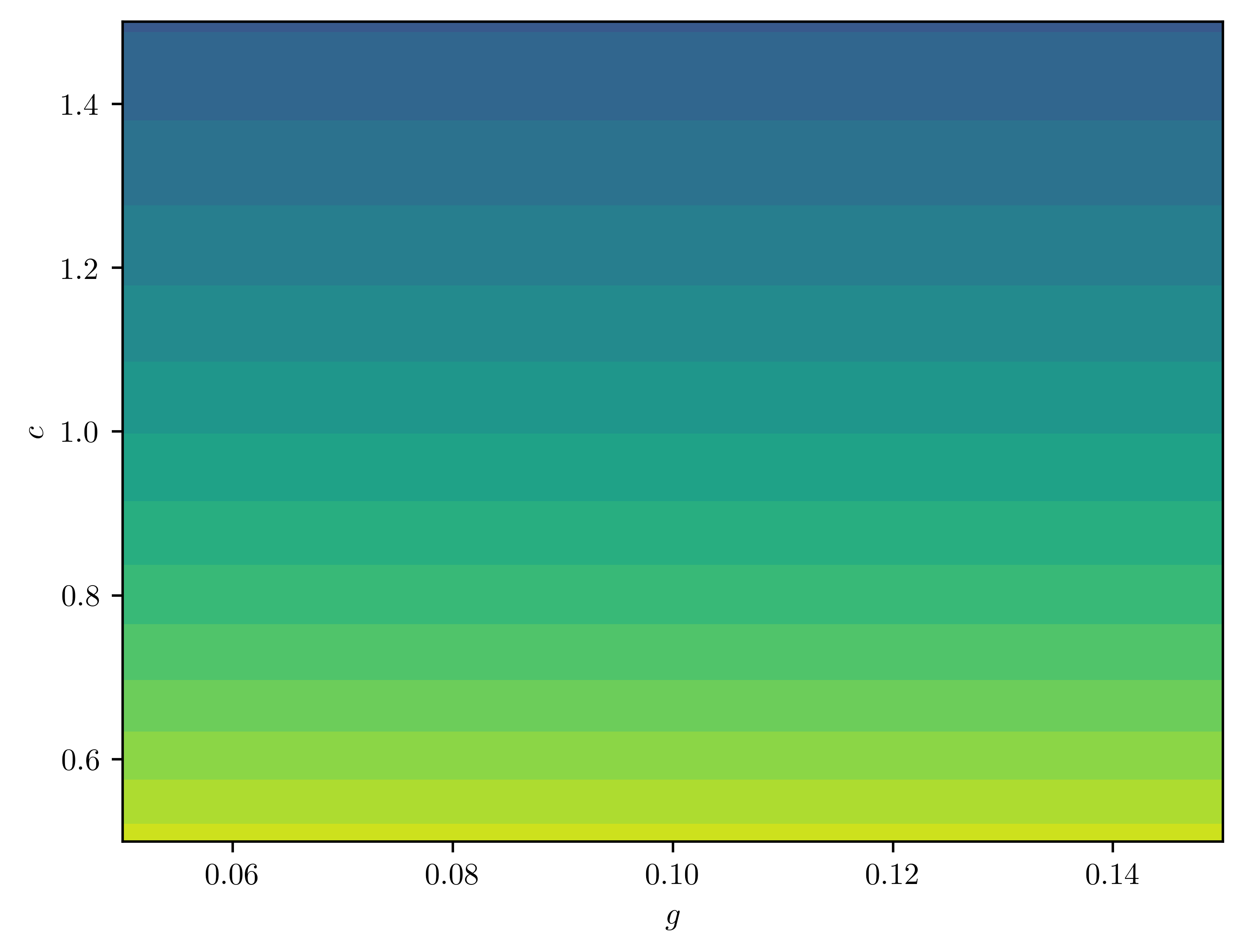
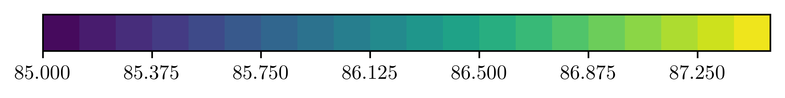
(a) Expected information gain $\overline{\Phi}_{\rm KL}$

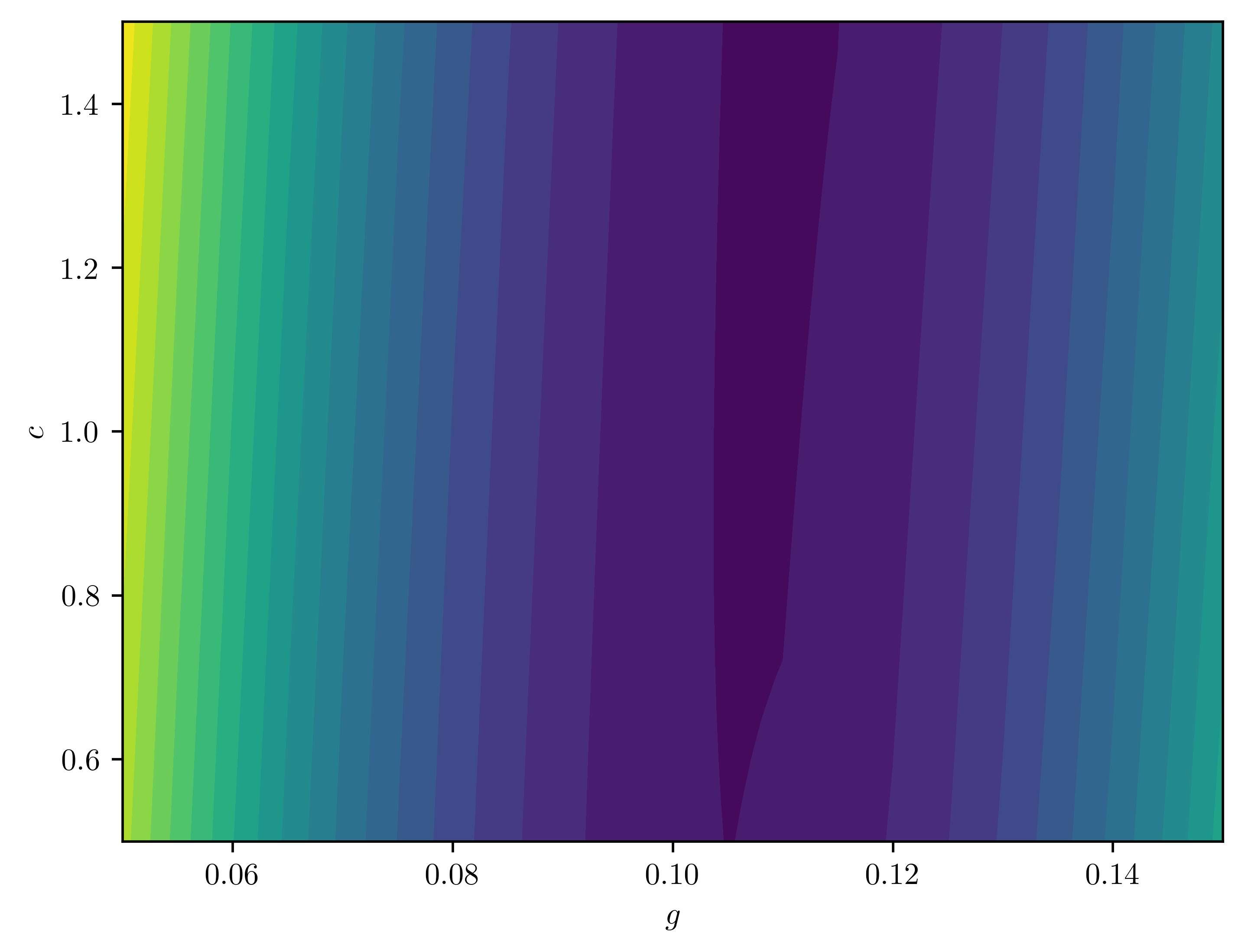
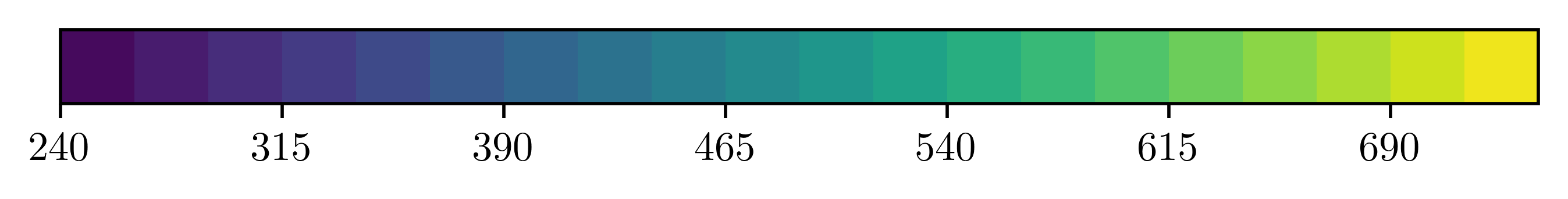
(b) Information Gain $\Phi_{\rm KL}$

Figure 2: $\Phi_{\rm KL}$ and $\overline{\Phi}_{\rm KL}$ as functions of $c$ and $g$. Note the difference in scales and that $\overline{\Phi}_{\rm KL}$ is independent of $g$.

We note that the information gain varies strongly as a function of $g$. This sensitivity is not unexpected from this model, because $g$ influences flow through the boundary. Moreover, since $g$ is a boundary source term that enters the governing equations linearly, it does not appear in the Hessian (18a). Therefore, the influence of $g$ on the information gain is solely coming from the third term in (21). In particular, the expected information gain is independent of $g$ as can be seen in Figure 2. Moreover, note that $\Phi_{\rm KL}$, when considered as a function of $g$, has a local minimum at which the sensitivity vanishes. From observing this local sensitivity, one may draw the incorrect conclusion that $\Phi_{\rm KL}$ is generally insensitive to $g$. In such a case, a global sensitivity analysis, as demonstrated in the next section, is a more accurate description.

4.2 Fault-Slip Inversion in 3D

In this section, we apply the proposed methods to a three-dimensional model problem inspired from the field of seismology. Namely, we consider the setting of linear elasticity to describe the deformation of the earth’s crust due to tectonic activity. An important inverse problem in this context is that of inferring the slip pattern along a tectonic fault based on observations of the surface deformation. The specific problem we study is adapted from [23]. Although our model is merely a synthetic example, it is representative of the type of inverse problem our methods are intended to analyze.

4.2.1 Forward Model

Consider a triangular prism domain $\Omega\subset\mathbb{R}^{3}$ with boundary $\Gamma=\Gamma_{b}\cup\Gamma_{k}\cup\Gamma_{t}\cup\Gamma_{s}$, where $\Gamma_{b},\Gamma_{k},\Gamma_{t}$, and $\Gamma_{s}$ are the bottom, back, top and the side surfaces, respectively; see Figure 3 for a visualization of the domain. We would like to infer the slip along $\Gamma_{b}$, denoted by $\textstyle{m}$, based on point observations of the displacement on the top surface $\Gamma_{t}$. We assume a linear elasticity model for the displacement ${\mathchoice{\mbox{\boldmath$\displaystyle{u}$}}{\mbox{\boldmath$\textstyle{u}$}}{\mbox{\boldmath$\scriptstyle{u}$}}{\mbox{\boldmath$\scriptscriptstyle{u}$}}}=[u_{1}\;u_{2}\;u_{3}]^{\top}\in H^{1}(\Omega)^{3}$:

$$-\nabla\cdot{\mathchoice{\mbox{\boldmath$\displaystyle{\sigma}$}}{\mbox{\boldmath$\textstyle{\sigma}$}}{\mbox{\boldmath$\scriptstyle{\sigma}$}}{\mbox{\boldmath$\scriptscriptstyle{\sigma}$}}}({\mathchoice{\mbox{\boldmath$\displaystyle{u}$}}{\mbox{\boldmath$\textstyle{u}$}}{\mbox{\boldmath$\scriptstyle{u}$}}{\mbox{\boldmath$\scriptscriptstyle{u}$}}})={\mathchoice{\mbox{\boldmath$\displaystyle{0}$}}{\mbox{\boldmath$\textstyle{0}$}}{\mbox{\boldmath$\scriptstyle{0}$}}{\mbox{\boldmath$\scriptscriptstyle{0}$}}},\qquad\text{ in }\Omega,$$ (50)

where ${\mathchoice{\mbox{\boldmath$\displaystyle{\sigma}$}}{\mbox{\boldmath$\textstyle{\sigma}$}}{\mbox{\boldmath$\scriptstyle{\sigma}$}}{\mbox{\boldmath$\scriptscriptstyle{\sigma}$}}}({\mathchoice{\mbox{\boldmath$\displaystyle{u}$}}{\mbox{\boldmath$\textstyle{u}$}}{\mbox{\boldmath$\scriptstyle{u}$}}{\mbox{\boldmath$\scriptscriptstyle{u}$}}})\mathrel{\mathop{\ordinarycolon}}=\mathbb{C}{\mathchoice{\mbox{\boldmath$\displaystyle{\varepsilon}$}}{\mbox{\boldmath$\textstyle{\varepsilon}$}}{\mbox{\boldmath$\scriptstyle{\varepsilon}$}}{\mbox{\boldmath$\scriptscriptstyle{\varepsilon}$}}}({\mathchoice{\mbox{\boldmath$\displaystyle{u}$}}{\mbox{\boldmath$\textstyle{u}$}}{\mbox{\boldmath$\scriptstyle{u}$}}{\mbox{\boldmath$\scriptscriptstyle{u}$}}})=2\mu{\mathchoice{\mbox{\boldmath$\displaystyle{\varepsilon({\mathchoice{\mbox{\boldmath$\displaystyle{u}$}}{\mbox{\boldmath$\textstyle{u}$}}{\mbox{\boldmath$\scriptstyle{u}$}}{\mbox{\boldmath$\scriptscriptstyle{u}$}}})}$}}{\mbox{\boldmath$\textstyle{\varepsilon({\mathchoice{\mbox{\boldmath$\displaystyle{u}$}}{\mbox{\boldmath$\textstyle{u}$}}{\mbox{\boldmath$\scriptstyle{u}$}}{\mbox{\boldmath$\scriptscriptstyle{u}$}}})}$}}{\mbox{\boldmath$\scriptstyle{\varepsilon({\mathchoice{\mbox{\boldmath$\displaystyle{u}$}}{\mbox{\boldmath$\textstyle{u}$}}{\mbox{\boldmath$\scriptstyle{u}$}}{\mbox{\boldmath$\scriptscriptstyle{u}$}}})}$}}{\mbox{\boldmath$\scriptscriptstyle{\varepsilon({\mathchoice{\mbox{\boldmath$\displaystyle{u}$}}{\mbox{\boldmath$\textstyle{u}$}}{\mbox{\boldmath$\scriptstyle{u}$}}{\mbox{\boldmath$\scriptscriptstyle{u}$}}})}$}}}+\lambda\text{tr}({\mathchoice{\mbox{\boldmath$\displaystyle{\varepsilon}$}}{\mbox{\boldmath$\textstyle{\varepsilon}$}}{\mbox{\boldmath$\scriptstyle{\varepsilon}$}}{\mbox{\boldmath$\scriptscriptstyle{\varepsilon}$}}}({\mathchoice{\mbox{\boldmath$\displaystyle{u}$}}{\mbox{\boldmath$\textstyle{u}$}}{\mbox{\boldmath$\scriptstyle{u}$}}{\mbox{\boldmath$\scriptscriptstyle{u}$}}}))\mathbf{I}$ is the fourth-order linear elasticity stress tensor and ${\mathchoice{\mbox{\boldmath$\displaystyle{\varepsilon}$}}{\mbox{\boldmath$\textstyle{\varepsilon}$}}{\mbox{\boldmath$\scriptstyle{\varepsilon}$}}{\mbox{\boldmath$\scriptscriptstyle{\varepsilon}$}}}({\mathchoice{\mbox{\boldmath$\displaystyle{u}$}}{\mbox{\boldmath$\textstyle{u}$}}{\mbox{\boldmath$\scriptstyle{u}$}}{\mbox{\boldmath$\scriptscriptstyle{u}$}}})\mathrel{\mathop{\ordinarycolon}}=\frac{1}{2}\left(\nabla{\mathchoice{\mbox{\boldmath$\displaystyle{u}$}}{\mbox{\boldmath$\textstyle{u}$}}{\mbox{\boldmath$\scriptstyle{u}$}}{\mbox{\boldmath$\scriptscriptstyle{u}$}}}+(\nabla{\mathchoice{\mbox{\boldmath$\displaystyle{u}$}}{\mbox{\boldmath$\textstyle{u}$}}{\mbox{\boldmath$\scriptstyle{u}$}}{\mbox{\boldmath$\scriptscriptstyle{u}$}}})^{T}\right)$ is the strain tensor. The stress tensor involves the Láme parameters $\{\mu,\lambda\}$ describing material properties. Specifying the boundary conditions, we have:

$$-\nabla\cdot[\mu(\nabla{\mathchoice{\mbox{\boldmath$\displaystyle{u}$}}{\mbox{\boldmath$\textstyle{u}$}}{\mbox{\boldmath$\scriptstyle{u}$}}{\mbox{\boldmath$\scriptscriptstyle{u}$}}}+(\nabla{\mathchoice{\mbox{\boldmath$\displaystyle{u}$}}{\mbox{\boldmath$\textstyle{u}$}}{\mbox{\boldmath$\scriptstyle{u}$}}{\mbox{\boldmath$\scriptscriptstyle{u}$}}})^{T})+\lambda\nabla\cdot{\mathchoice{\mbox{\boldmath$\displaystyle{u}$}}{\mbox{\boldmath$\textstyle{u}$}}{\mbox{\boldmath$\scriptstyle{u}$}}{\mbox{\boldmath$\scriptscriptstyle{u}$}}}\mathbf{I}] ={\mathchoice{\mbox{\boldmath$\displaystyle{0}$}}{\mbox{\boldmath$\textstyle{0}$}}{\mbox{\boldmath$\scriptstyle{0}$}}{\mbox{\boldmath$\scriptscriptstyle{0}$}}} \text{ in }\Omega,$$ (51a)

$${\mathchoice{\mbox{\boldmath$\displaystyle{\sigma}$}}{\mbox{\boldmath$\textstyle{\sigma}$}}{\mbox{\boldmath$\scriptstyle{\sigma}$}}{\mbox{\boldmath$\scriptscriptstyle{\sigma}$}}}({\mathchoice{\mbox{\boldmath$\displaystyle{u}$}}{\mbox{\boldmath$\textstyle{u}$}}{\mbox{\boldmath$\scriptstyle{u}$}}{\mbox{\boldmath$\scriptscriptstyle{u}$}}}){\mathchoice{\mbox{\boldmath$\displaystyle{n}$}}{\mbox{\boldmath$\textstyle{n}$}}{\mbox{\boldmath$\scriptstyle{n}$}}{\mbox{\boldmath$\scriptscriptstyle{n}$}}} =0 \text{ on }\Gamma_{t},$$ (51b)

$${\mathchoice{\mbox{\boldmath$\displaystyle{u}$}}{\mbox{\boldmath$\textstyle{u}$}}{\mbox{\boldmath$\scriptstyle{u}$}}{\mbox{\boldmath$\scriptscriptstyle{u}$}}}+\beta_{k}{\mathchoice{\mbox{\boldmath$\displaystyle{\sigma(u)n}$}}{\mbox{\boldmath$\textstyle{\sigma(u)n}$}}{\mbox{\boldmath$\scriptstyle{\sigma(u)n}$}}{\mbox{\boldmath$\scriptscriptstyle{\sigma(u)n}$}}} ={\mathchoice{\mbox{\boldmath$\displaystyle{0}$}}{\mbox{\boldmath$\textstyle{0}$}}{\mbox{\boldmath$\scriptstyle{0}$}}{\mbox{\boldmath$\scriptscriptstyle{0}$}}} \text{ on }\Gamma_{k},$$ (51c)

$${\mathchoice{\mbox{\boldmath$\displaystyle{u}$}}{\mbox{\boldmath$\textstyle{u}$}}{\mbox{\boldmath$\scriptstyle{u}$}}{\mbox{\boldmath$\scriptscriptstyle{u}$}}}+\beta_{s}{\mathchoice{\mbox{\boldmath$\displaystyle{\sigma(u)n}$}}{\mbox{\boldmath$\textstyle{\sigma(u)n}$}}{\mbox{\boldmath$\scriptstyle{\sigma(u)n}$}}{\mbox{\boldmath$\scriptscriptstyle{\sigma(u)n}$}}} ={\mathchoice{\mbox{\boldmath$\displaystyle{h}$}}{\mbox{\boldmath$\textstyle{h}$}}{\mbox{\boldmath$\scriptstyle{h}$}}{\mbox{\boldmath$\scriptscriptstyle{h}$}}} \text{ on }\Gamma_{s},$$ (51d)

$${\mathchoice{\mbox{\boldmath$\displaystyle{u}$}}{\mbox{\boldmath$\textstyle{u}$}}{\mbox{\boldmath$\scriptstyle{u}$}}{\mbox{\boldmath$\scriptscriptstyle{u}$}}}\cdot{\mathchoice{\mbox{\boldmath$\displaystyle{n}$}}{\mbox{\boldmath$\textstyle{n}$}}{\mbox{\boldmath$\scriptstyle{n}$}}{\mbox{\boldmath$\scriptscriptstyle{n}$}}} =0 \text{ on }\Gamma_{b},$$ (51e)

$$\delta\mathbf{T}({\mathchoice{\mbox{\boldmath$\displaystyle{\sigma}$}}{\mbox{\boldmath$\textstyle{\sigma}$}}{\mbox{\boldmath$\scriptstyle{\sigma}$}}{\mbox{\boldmath$\scriptscriptstyle{\sigma}$}}}({\mathchoice{\mbox{\boldmath$\displaystyle{u}$}}{\mbox{\boldmath$\textstyle{u}$}}{\mbox{\boldmath$\scriptstyle{u}$}}{\mbox{\boldmath$\scriptscriptstyle{u}$}}}){\mathchoice{\mbox{\boldmath$\displaystyle{n}$}}{\mbox{\boldmath$\textstyle{n}$}}{\mbox{\boldmath$\scriptstyle{n}$}}{\mbox{\boldmath$\scriptscriptstyle{n}$}}})+\mathbf{T}{\mathchoice{\mbox{\boldmath$\displaystyle{u}$}}{\mbox{\boldmath$\textstyle{u}$}}{\mbox{\boldmath$\scriptstyle{u}$}}{\mbox{\boldmath$\scriptscriptstyle{u}$}}} ={\mathchoice{\mbox{\boldmath$\displaystyle{m}$}}{\mbox{\boldmath$\textstyle{m}$}}{\mbox{\boldmath$\scriptstyle{m}$}}{\mbox{\boldmath$\scriptscriptstyle{m}$}}} \text{ on }\Gamma_{b}.$$ (51f)

Here, $\mathbf{T}$ is the operator that extracts the tangential components of a vector, i.e., $\mathbf{T}{\mathchoice{\mbox{\boldmath$\displaystyle{u}$}}{\mbox{\boldmath$\textstyle{u}$}}{\mbox{\boldmath$\scriptstyle{u}$}}{\mbox{\boldmath$\scriptscriptstyle{u}$}}}\vcentcolon=(\mathbf{I}-{\mathchoice{\mbox{\boldmath$\displaystyle{n}$}}{\mbox{\boldmath$\textstyle{n}$}}{\mbox{\boldmath$\scriptstyle{n}$}}{\mbox{\boldmath$\scriptscriptstyle{n}$}}}\otimes{\mathchoice{\mbox{\boldmath$\displaystyle{n}$}}{\mbox{\boldmath$\textstyle{n}$}}{\mbox{\boldmath$\scriptstyle{n}$}}{\mbox{\boldmath$\scriptscriptstyle{n}$}}}){\mathchoice{\mbox{\boldmath$\displaystyle{u}$}}{\mbox{\boldmath$\textstyle{u}$}}{\mbox{\boldmath$\scriptstyle{u}$}}{\mbox{\boldmath$\scriptscriptstyle{u}$}}}={\mathchoice{\mbox{\boldmath$\displaystyle{u}$}}{\mbox{\boldmath$\textstyle{u}$}}{\mbox{\boldmath$\scriptstyle{u}$}}{\mbox{\boldmath$\scriptscriptstyle{u}$}}}-({\mathchoice{\mbox{\boldmath$\displaystyle{n}$}}{\mbox{\boldmath$\textstyle{n}$}}{\mbox{\boldmath$\scriptstyle{n}$}}{\mbox{\boldmath$\scriptscriptstyle{n}$}}}^{T}{\mathchoice{\mbox{\boldmath$\displaystyle{u}$}}{\mbox{\boldmath$\textstyle{u}$}}{\mbox{\boldmath$\scriptstyle{u}$}}{\mbox{\boldmath$\scriptscriptstyle{u}$}}}){\mathchoice{\mbox{\boldmath$\displaystyle{n}$}}{\mbox{\boldmath$\textstyle{n}$}}{\mbox{\boldmath$\scriptstyle{n}$}}{\mbox{\boldmath$\scriptscriptstyle{n}$}}}$, where $\textstyle{n}$ is the unit normal of the domain. The Robin-type condition (51f) can be understood as regularized Dirichlet condition with parameter $0<\delta\ll 1$.

To model the heterogeneous properties of the earth, we use spatially varying Láme parameters. We assume these parameters to have variations only in vertical direction modeling a layered earth structure. Specifically, we define the Láme parameters using the expansions

$$\lambda(y)=\overline{\lambda}+\sum_{i=1}^{6}e_{i}(y)\lambda_{i}^{\rm KL}\qquad\text{and}\qquad\mu(y)=\overline{\mu}+\sum_{i=1}^{6}e_{i}(y)\mu_{i}^{\rm KL}.$$ (52)

This representation is motivated by the truncated Karhunen–Loève (KL) expansion, hence the choice of superscript $\mathrm{KL}$ in the above representation. In these equations, $e_{i}$’s are suitably scaled KL basis functions, computed as described in [22]. For the purposes of the present study, the coefficients $\{\lambda_{i}^{\rm KL}\}$ and $\{\mu_{i}^{\rm KL}\}$ are (fixed) random draws from a standard normal distribution. To illustrate, we show the corresponding realization of the $\lambda$ field in Figure 3 (right). As for the remaining auxiliary parameters, we assume the nominal values of $\overline{\lambda}=2.0,\overline{\mu}=2.50,\beta_{k}=10^{-4}$, and $\beta_{s}=10^{-4}$.

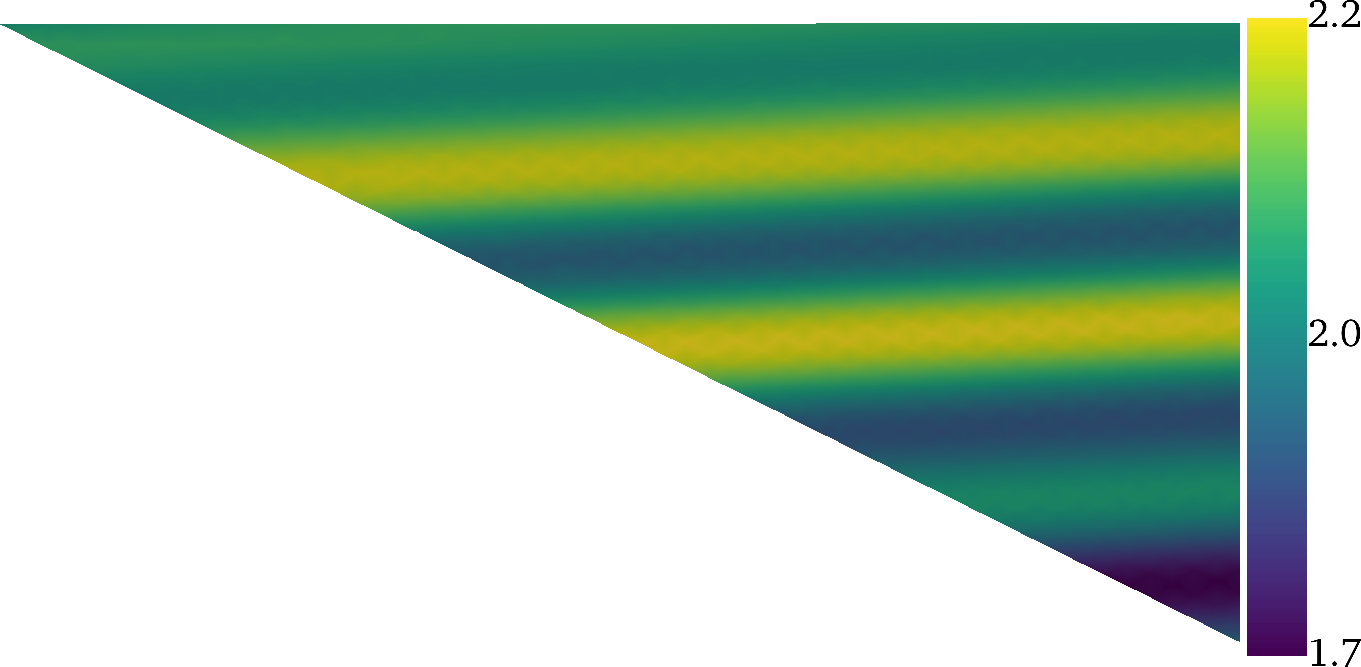
Figure 3: (Left) Visualization of $\Omega$. (Right) Realization of $\lambda$ with six KL modes.

4.2.2 Inverse Problem Setup

Now we return to the inverse problem under study. We seek to infer the fault slip $\textstyle{m}$ and compute the sensitivity of the information gain with respect to the auxiliary parameters $\beta,\overline{\mu},\{\mu_{i}^{\rm KL}\},\overline{\lambda}$, and $\{\lambda_{i}^{\rm KL}\}$. To cast the problem into the abstract setup developed in Section 3, we consider the weak form of the governing PDE. Defining the function space ${\mathchoice{\mbox{\boldmath$\displaystyle{V}$}}{\mbox{\boldmath$\textstyle{V}$}}{\mbox{\boldmath$\scriptstyle{V}$}}{\mbox{\boldmath$\scriptscriptstyle{V}$}}}\vcentcolon=\{{\mathchoice{\mbox{\boldmath$\displaystyle{u}$}}{\mbox{\boldmath$\textstyle{u}$}}{\mbox{\boldmath$\scriptstyle{u}$}}{\mbox{\boldmath$\scriptscriptstyle{u}$}}}\in H^{1}(\Omega)^{3}\mathrel{\mathop{\ordinarycolon}}{\mathchoice{\mbox{\boldmath$\displaystyle{u}$}}{\mbox{\boldmath$\textstyle{u}$}}{\mbox{\boldmath$\scriptstyle{u}$}}{\mbox{\boldmath$\scriptscriptstyle{u}$}}}\cdot{\mathchoice{\mbox{\boldmath$\displaystyle{n}$}}{\mbox{\boldmath$\textstyle{n}$}}{\mbox{\boldmath$\scriptstyle{n}$}}{\mbox{\boldmath$\scriptscriptstyle{n}$}}}=0\text{ on }\Gamma_{b}\}$, the weak form of (51) is as follows: find ${\mathchoice{\mbox{\boldmath$\displaystyle{u}$}}{\mbox{\boldmath$\textstyle{u}$}}{\mbox{\boldmath$\scriptstyle{u}$}}{\mbox{\boldmath$\scriptscriptstyle{u}$}}}\in\mathbf{V}$ such that for every ${\mathchoice{\mbox{\boldmath$\displaystyle{p}$}}{\mbox{\boldmath$\textstyle{p}$}}{\mbox{\boldmath$\scriptstyle{p}$}}{\mbox{\boldmath$\scriptscriptstyle{p}$}}}\in{\mathchoice{\mbox{\boldmath$\displaystyle{V}$}}{\mbox{\boldmath$\textstyle{V}$}}{\mbox{\boldmath$\scriptstyle{V}$}}{\mbox{\boldmath$\scriptscriptstyle{V}$}}}$

$$\int_{\Gamma_{k}}\beta^{-1}_{k}{\mathchoice{\mbox{\boldmath$\displaystyle{u}$}}{\mbox{\boldmath$\textstyle{u}$}}{\mbox{\boldmath$\scriptstyle{u}$}}{\mbox{\boldmath$\scriptscriptstyle{u}$}}}\cdot{\mathchoice{\mbox{\boldmath$\displaystyle{p}$}}{\mbox{\boldmath$\textstyle{p}$}}{\mbox{\boldmath$\scriptstyle{p}$}}{\mbox{\boldmath$\scriptscriptstyle{p}$}}}\differential{s}+\int_{\Gamma_{s}}\beta^{-1}_{s}{\mathchoice{\mbox{\boldmath$\displaystyle{u}$}}{\mbox{\boldmath$\textstyle{u}$}}{\mbox{\boldmath$\scriptstyle{u}$}}{\mbox{\boldmath$\scriptscriptstyle{u}$}}}\cdot{\mathchoice{\mbox{\boldmath$\displaystyle{p}$}}{\mbox{\boldmath$\textstyle{p}$}}{\mbox{\boldmath$\scriptstyle{p}$}}{\mbox{\boldmath$\scriptscriptstyle{p}$}}}\differential{s}+\int_{\Gamma_{b}}\delta^{-1}\mathbf{T}{\mathchoice{\mbox{\boldmath$\displaystyle{u}$}}{\mbox{\boldmath$\textstyle{u}$}}{\mbox{\boldmath$\scriptstyle{u}$}}{\mbox{\boldmath$\scriptscriptstyle{u}$}}}\cdot{\mathchoice{\mbox{\boldmath$\displaystyle{p}$}}{\mbox{\boldmath$\textstyle{p}$}}{\mbox{\boldmath$\scriptstyle{p}$}}{\mbox{\boldmath$\scriptscriptstyle{p}$}}}\differential{s}+\int_{\Omega}\varepsilon({\mathchoice{\mbox{\boldmath$\displaystyle{u}$}}{\mbox{\boldmath$\textstyle{u}$}}{\mbox{\boldmath$\scriptstyle{u}$}}{\mbox{\boldmath$\scriptscriptstyle{u}$}}})\mathrel{\mathop{\ordinarycolon}}\mathbb{C}[\varepsilon({\mathchoice{\mbox{\boldmath$\displaystyle{p}$}}{\mbox{\boldmath$\textstyle{p}$}}{\mbox{\boldmath$\scriptstyle{p}$}}{\mbox{\boldmath$\scriptscriptstyle{p}$}}})]\differential{x}-\int_{\Gamma_{b}}\delta^{-1}{\mathchoice{\mbox{\boldmath$\displaystyle{m}$}}{\mbox{\boldmath$\textstyle{m}$}}{\mbox{\boldmath$\scriptstyle{m}$}}{\mbox{\boldmath$\scriptscriptstyle{m}$}}}\cdot{\mathchoice{\mbox{\boldmath$\displaystyle{p}$}}{\mbox{\boldmath$\textstyle{p}$}}{\mbox{\boldmath$\scriptstyle{p}$}}{\mbox{\boldmath$\scriptscriptstyle{p}$}}}\differential{s}-\int_{\Gamma_{s}}\beta_{s}^{-1}{\mathchoice{\mbox{\boldmath$\displaystyle{h}$}}{\mbox{\boldmath$\textstyle{h}$}}{\mbox{\boldmath$\scriptstyle{h}$}}{\mbox{\boldmath$\scriptscriptstyle{h}$}}}\cdot{\mathchoice{\mbox{\boldmath$\displaystyle{p}$}}{\mbox{\boldmath$\textstyle{p}$}}{\mbox{\boldmath$\scriptstyle{p}$}}{\mbox{\boldmath$\scriptscriptstyle{p}$}}}\differential{s}=0.$$

Note that this fits into the abstract weak PDE formulation described in Section 2 (see (5)), and facilitates deploying the approach developed in Section 3.

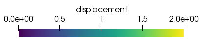
Figure 4: True slip field $\textstyle{m}$ given by (53) and slip MAP estimate $\textstyle{m}$. The background color shows the slip magnitude (which can also be seen from the length of the arrows).

For the synthetic data generation, we assume that the “ground-truth” fault slip has the form

$${\mathchoice{\mbox{\boldmath$\displaystyle{m}$}}{\mbox{\boldmath$\textstyle{m}$}}{\mbox{\boldmath$\scriptstyle{m}$}}{\mbox{\boldmath$\scriptscriptstyle{m}$}}}(x,y,z)=\begin{pmatrix}\exp\left[(x+1.25)^{2}+(z-0.5)^{2}\right]\\ 0\\ 2\exp\left[(x+1.25)^{2}+(z-0.5)^{2}\right]\\ \end{pmatrix}.$$ (53)

See Figure 4 (left) for a visualization of this ground-truth parameter. We solve our forward model (51) with this slip field and our nominal set of parameters to compute the “truth” displacement field ${\mathchoice{\mbox{\boldmath$\displaystyle{u}$}}{\mbox{\boldmath$\textstyle{u}$}}{\mbox{\boldmath$\scriptstyle{u}$}}{\mbox{\boldmath$\scriptscriptstyle{u}$}}}^{\rm true}$, which is shown on the left in Figure 5. We then take point measurements on $\Gamma_{t}$, the top surface of the domain at $N_{\text{obs}}=32$ measurement locations, spaced uniformly on an $8\times 4$ a grid on $\Gamma_{t}$. We add independent additive noise with the standard deviation $\sigma=0.001$ to this measurement data to obtain synthetic observations $\mathbf{u}^{\text{obs}}$.

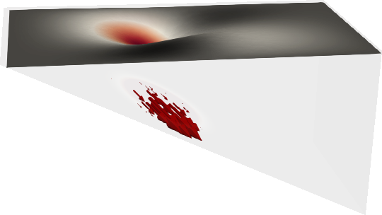
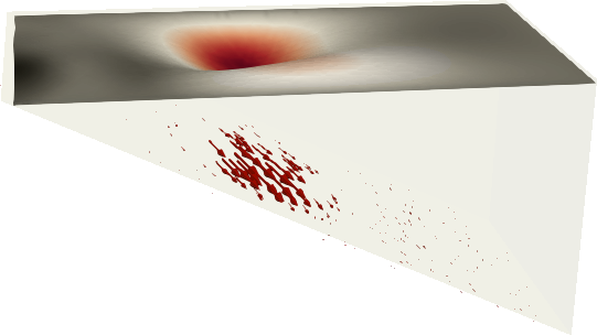
Figure 5: Fault slip (red arrows) and corresponding deformation on the top surface $\Gamma_{t}$. Shown on the left is the result for the truth fault slip used to generate synthetic data, and on the right the MAP fault slip.

Next, we discuss the prior measure. We use a Gaussian measure with mean $m_{\text{prior}}={\mathchoice{\mbox{\boldmath$\displaystyle{0}$}}{\mbox{\boldmath$\textstyle{0}$}}{\mbox{\boldmath$\scriptstyle{0}$}}{\mbox{\boldmath$\scriptscriptstyle{0}$}}}$, and a squared inverse elliptic operator as the covariance. Specifically, $\mathcal{C}_{\text{prior}}=\mathcal{S}^{-2}$, where $\mathcal{S}$ is the solution operator mapping $\textstyle{s}$ to $\textstyle{m}$ for the following PDE given in weak form as:

$$\int_{\Gamma_{b}}\gamma_{\text{pr}}\nabla{\mathchoice{\mbox{\boldmath$\displaystyle{m}$}}{\mbox{\boldmath$\textstyle{m}$}}{\mbox{\boldmath$\scriptstyle{m}$}}{\mbox{\boldmath$\scriptscriptstyle{m}$}}}\cdot\nabla{\mathchoice{\mbox{\boldmath$\displaystyle{p}$}}{\mbox{\boldmath$\textstyle{p}$}}{\mbox{\boldmath$\scriptstyle{p}$}}{\mbox{\boldmath$\scriptscriptstyle{p}$}}}+\delta_{\text{pr}}{\mathchoice{\mbox{\boldmath$\displaystyle{m}$}}{\mbox{\boldmath$\textstyle{m}$}}{\mbox{\boldmath$\scriptstyle{m}$}}{\mbox{\boldmath$\scriptscriptstyle{m}$}}}\cdot{\mathchoice{\mbox{\boldmath$\displaystyle{p}$}}{\mbox{\boldmath$\textstyle{p}$}}{\mbox{\boldmath$\scriptstyle{p}$}}{\mbox{\boldmath$\scriptscriptstyle{p}$}}}\differential{x}+\int_{\partial\Gamma_{b}}\beta_{\text{pr}}{\mathchoice{\mbox{\boldmath$\displaystyle{m}$}}{\mbox{\boldmath$\textstyle{m}$}}{\mbox{\boldmath$\scriptstyle{m}$}}{\mbox{\boldmath$\scriptscriptstyle{m}$}}}\cdot{\mathchoice{\mbox{\boldmath$\displaystyle{p}$}}{\mbox{\boldmath$\textstyle{p}$}}{\mbox{\boldmath$\scriptstyle{p}$}}{\mbox{\boldmath$\scriptscriptstyle{p}$}}}\differential{s}=\int_{\Gamma_{b}}{\mathchoice{\mbox{\boldmath$\displaystyle{s}$}}{\mbox{\boldmath$\textstyle{s}$}}{\mbox{\boldmath$\scriptstyle{s}$}}{\mbox{\boldmath$\scriptscriptstyle{s}$}}}\cdot{\mathchoice{\mbox{\boldmath$\displaystyle{p}$}}{\mbox{\boldmath$\textstyle{p}$}}{\mbox{\boldmath$\scriptstyle{p}$}}{\mbox{\boldmath$\scriptscriptstyle{p}$}}}\differential{x},\qquad\forall{\mathchoice{\mbox{\boldmath$\displaystyle{p}$}}{\mbox{\boldmath$\textstyle{p}$}}{\mbox{\boldmath$\scriptstyle{p}$}}{\mbox{\boldmath$\scriptscriptstyle{p}$}}}\in H^{1}(\Gamma_{b})^{2}.$$ (54)

In this formulation, $\gamma_{\text{pr}}$ and $\delta_{\text{pr}}$ govern the correlation length and pointwise variance of the prior samples, and $\beta_{\text{pr}}$ is a parameter stemming from an additional Robin boundary condition that is used to minimize boundary artifacts. This formulation of the prior is adapted from [32], and we choose the parameters $(\gamma_{\text{pr}},\delta_{\text{pr}})=(32,3.2)$ and $\beta_{\text{pr}}=\sqrt{\gamma_{\text{pr}}\delta_{\text{pr}}}/1.42$.

4.2.3 Numerical Results

We now solve the Bayesian inverse problem. In Figure 4, we show the MAP point, which differs from the true slip field as a consequence of the sparse measurements, the noise in the measurement data, and the prior assumptions. However, the solution of the Bayesian inverse problem is not the main focus here. Instead, we seek to understand the sensitivity of the information gain with respect to the auxiliary model parameters, using Algorithm 1. To facilitate this, we need to first parameterize the uncertainty in the different auxiliary parameters consistently. Suppose $\vartheta_{i}$, $i=1,\ldots,n$, are the auxiliary model parameters. Then, $\vartheta_{i}$ represents KL coefficients $\overline{\lambda},\overline{\mu},\lambda_{i}^{\rm KL},\mu_{i}^{\rm KL}$ in the Láme parameters and coefficient $\beta_{k},\beta_{s}$ of the Robin conditions. Since we compare parameters with different physical units, we use the parameterization

$$\vartheta_{i}=(1+\alpha\theta_{i})\overline{\vartheta}_{i},\quad i\in\{1,\ldots,n\},$$ (55)

where $\overline{\vartheta}_{i}$’s are the nominal values, $\alpha>0$ is a coefficient modeling our uncertainty level in the nominal value, and $\theta_{i}$ is the perturbation parameter we study in place of $\vartheta_{i}$. Note that this parameterization assumes the nominal parameter values are nonzero. We assume $\theta_{i}\in[-1,1]$ and let $\alpha=0.05$, i.e., we consider an uncertainty level of $5\%$ for each auxiliary parameter. The present parameterization also sets the stage for a global sensitivity analysis, where $\theta_{i}$ will be assumed uniformly distributed random variables on the interval $[-1,1]$.

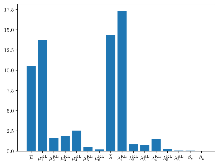
(a) Information Gain Sensitivities

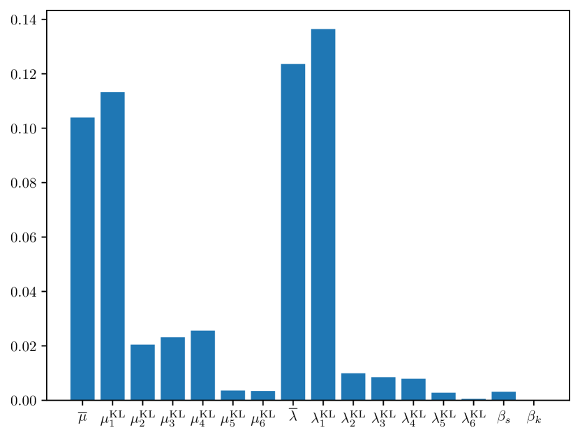
(b) Expected Information Gain Sensitivities

Figure 6: Sensitivity of the KL divergence and its expectation over data with respect to auxiliary parameters.

We use Algorithm 1 to compute the sensitivities of the information gain and its expectation over data with respect to the auxiliary parameters. The results are reported in Figure 6. We find that the Láme parameters hold significantly more sensitivity than the $\beta$ parameters in the boundary conditions. Moreover, for both Láme parameters, the mean value and the first KL mode are the most influential. From an uncertainty quantification perspective, these results can be viewed as a positive for the well-foundedness of the model. Indeed, both $\beta$ parameters are numerical parameter that are used due to the truncation of the domain. Furthermore, the sensitivity being dominated by the first KL modes indicates that, for this model, it may be acceptable to ignore more oscillatory modes of the Láme parameters as long as the mean is correctly chosen in the first place.

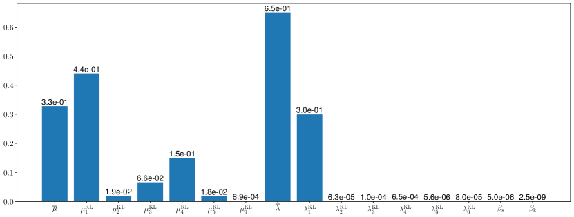
Figure 7: Derivative-based Sobol indices of the information gain with respect to the auxiliary parameters for the elasticity model.

Finally, we study the global sensitivity of the information gain with respect to the auxiliary parameters. As discussed in Section 2.4, this can be done by considering the derivative-based upper bounds on the total Sobol indices. The integrals in eq. 27 are approximated via sample averaging. A sample of size 200 was found to be sufficient for the integral of the derivatives, whereas the total variance was estimated with 500 samples. We report the computed Sobol index bounds in Figure 7. These results are generally consistent with the behavior seen in the local sensitivity results in Figure 6. In particular, both $\beta$ coefficients and the higher order KL modes, except $\mu_{4}^{\mathrm{KL}}$, are unimportant.

5 Conclusion

In this article, we have outlined a scalable approach for sensitivity analysis of the information gain and expected information gain with respect to auxiliary model parameters. Our approach builds on low-rank spectral decompositions, adjoint-based eigenvalue sensitivity analysis, and concepts from post-optimal sensitivity analysis. As seen in our computational examples, the (expected) information gain can exhibit complex dependence on auxiliary model parameters. This makes a practical sensitivity analysis framework important. The present work makes a foundational step in this direction.

A natural next step is extending the presented sensitivity analysis framework to the case of nonlinear Bayesian inverse problems. A possible approach is to utilize a Laplace approximation to the posterior. The present approach can be adapted to that setting. Though, it will be important to assess the extent to which the sensitivity of the Laplace approximation to the posterior with respect to the auxiliary parameters is indicative of the sensitivity of the true posterior distribution to these parameters.

The proposed sensitivity analysis framework is also synergistic to efforts in the area of Bayesian optimal experimental design (OED) [9, 1] and OED under uncertainty [18, 4, 10, 3]. Specifically, for OED under uncertainty, sensitivity analysis can reveal the most influential uncertain auxiliary parameters. Then, the OED problem may be formulated by focusing only on the most important auxiliary parameters. This process can potentially reduce the computational burden of OED under uncertainty substantially. Investigating such parameter dimension reduction approaches in the context of OED under uncertainty is an interesting area of future work.

6 Acknowledgment

The work of A. Alexanderian and A. Chowdhary was supported in part by US National Science Foundation grant DMS-2111044. The authors would also like to thank Tucker Hartland and Noemi Petra for their help in the slip inference computational example.

References

- [1] Alen Alexanderian “Optimal experimental design for infinite-dimensional Bayesian inverse problems governed by PDEs: A review” In Inverse Problems 37.4 IOP Publishing, 2021, pp. 043001
- [2] Alen Alexanderian, Philip J. Gloor and Omar Ghattas “On Bayesian A and D-Optimal Experimental Designs in Infinite Dimensions” In Bayesian Analysis 11.3, 2016 DOI: 10.1214/15-BA969
- [3] Alen Alexanderian, Ruanui Nicholson and Noemi Petra “Optimal design of large-scale nonlinear Bayesian inverse problems under model uncertainty” In arXiv preprint arXiv:2211.03952, 2022
- [4] Alen Alexanderian, Noemi Petra, Georg Stadler and Isaac Sunseri “Optimal design of large-scale Bayesian linear inverse problems under reducible model uncertainty: good to know what you don’t know” In SIAM/ASA J. Uncertain. Quantif. 9.1 SIAM, 2021, pp. 163–184
- [5] Alen Alexanderian and Arvind K. Saibaba “Efficient D-Optimal Design of Experiments for Infinite-Dimensional Bayesian Linear Inverse Problems” In SIAM Journal on Scientific Computing 40.5 Society for Industrial & Applied Mathematics (SIAM), 2018, pp. A2956–A2985 DOI: 10.1137/17m115712x
- [6] Kerstin Brandes and Roland Griesse “Quantitative stability analysis of optimal solutions in PDE-constrained optimization” In Journal of computational and applied mathematics 206.2 Elsevier, 2007, pp. 908–926
- [7] Tan Bui-Thanh, Omar Ghattas, James Martin and Georg Stadler “A Computational Framework for Infinite-Dimensional Bayesian Inverse Problems Part I: The Linearized Case, with Application to Global Seismic Inversion” In SIAM Journal on Scientific Computing 35.6, 2013, pp. A2494–A2523 DOI: 10.1137/12089586X
- [8] Kathryn Chaloner and Isabella Verdinelli “Bayesian experimental design: A review” In Statistical science JSTOR, 1995, pp. 273–304
- [9] Kathryn Chaloner and Isabella Verdinelli “Bayesian experimental design: A review” In Statistical Science 10.3, 1995, pp. 273–304
- [10] Chi Feng and Youssef M Marzouk “A layered multiple importance sampling scheme for focused optimal Bayesian experimental design” https://arxiv.org/abs/1903.11187 In preprint, 2019
- [11] Chi Feng and Youssef M. Marzouk “A layered multiple importance sampling scheme for focused optimal Bayesian experimental design” arXiv, 2019 DOI: 10.48550/ARXIV.1903.11187
- [12] Omar Ghattas and Karen Willcox “Learning physics-based models from data: perspectives from inverse problems and model reduction” In Acta Numerica 30, 2021, pp. 445–554
- [13] Alison L. Gibbs and Francis Edward Su “On Choosing and Bounding Probability Metrics” In International Statistical Review / Revue Internationale de Statistique 70.3 [Wiley, International Statistical Institute (ISI)], 2002, pp. 419–435
- [14] Roland Griesse “Stability and Sensitivity Analysis in Optimal Control of Partial Differential Equations”, Habilitation Thesis, Faculty of Natural Sciences, Karl-Franzens University, 2007
- [15] Max D. Gunzburger “Perspectives in Flow Control and Optimization” Society for IndustrialApplied Mathematics, 2002 DOI: 10.1137/1.9780898718720
- [16] Joseph Hart, Bart Bloemen Waanders and Roland Herzog “Hyper-Differential Sensitivity Analysis of Uncertain Parameters in PDE-Constrained Optimization” In International Journal for Uncertainty Quantification 10.3, 2020 DOI: 10.1615/Int.J.UncertaintyQuantification.2020032480
- [17] Diederik P Kingma and Max Welling “Auto-encoding variational Bayes” In arXiv preprint arXiv:1312.6114, 2013
- [18] Karina Koval, Alen Alexanderian and Georg Stadler “Optimal experimental design under irreducible uncertainty for linear inverse problems governed by PDEs” In Inverse Problems 36.7, 2020
- [19] Sergey Kucherenko and Bertrand Iooss “Derivative-Based Global Sensitivity Measures” In Handbook of Uncertainty Quantification Cham: Springer International Publishing, 2016, pp. 1–24 DOI: 10.1007/978-3-319-11259-6_36-1
- [20] S. Kullback and R.. Leibler “On Information and Sufficiency” In The Annals of Mathematical Statistics 22.1 Institute of Mathematical Statistics, 1951, pp. 79–86 DOI: 10.1214/aoms/1177729694
- [21] Peter D Lax “Linear algebra and its applications”, Pure and Applied Mathematics: A Wiley Series of Texts, Monographs and Tracts Chichester, England: Wiley-Blackwell, 2007
- [22] O.. Maitre and Omar M. Knio “Spectral Methods for Uncertainty Quantification” Springer Netherlands, 2010 DOI: 10.1007/978-90-481-3520-2
- [23] Kimberly McCormack “Earthquakes, groundwater and surface deformation : exploring the poroelastic response to megathrust earthquakes”, 2018
- [24] Noemi Petra and Georg Stadler “Model variational inverse problems governed by partial differential equations”, 2011
- [25] I.. Sobol “Estimation of the sensitivity of nonlinear mathematical models” In Mat. Model. 2.1, 1990, pp. 112–118
- [26] I.. Sobol “Global sensitivity indices for nonlinear mathematical models and their Monte Carlo estimates” The Second IMACS Seminar on Monte Carlo Methods (Varna, 1999) In Math. Comput. Simulation 55.1-3, 2001, pp. 271–280 DOI: 10.1016/S0378-4754(00)00270-6
- [27] I.M. Sobol’ and S. Kucherenko “Derivative based global sensitivity measures and their link with global sensitivity indices” In Mathematics and Computers in Simulation 79.10 Elsevier, 2009, pp. 3009–3017
- [28] A.. Stuart “Inverse problems: A Bayesian perspective” In Acta Numerica 19, 2010, pp. 451–559 DOI: 10.1017/S0962492910000061
- [29] Isaac Sunseri, Alen Alexanderian, Joseph Hart and Bart van Bloemen Waanders “Hyper-differential sensitivity analysis for nonlinear Bayesian inverse problems” In International Journal for Uncertainty Quantification Accepted, 2023
- [30] Isaac Sunseri, Joseph Hart, Bart van Bloemen Waanders and Alen Alexanderian “Hyper-Differential Sensitivity Analysis for Inverse Problems Constrained by Partial Differential Equations” In Inverse Problems 36.12, 2020, pp. 125001 DOI: 10.1088/1361-6420/abaf63
- [31] Naftali Tishby and Noga Zaslavsky “Deep learning and the information bottleneck principle” In 2015 IEEE Information Theory Workshop, 2015, pp. 1–5 IEEE
- [32] Umberto Villa, Noemi Petra and Omar Ghattas “HIPPYlib: an extensible software framework for large-scale inverse problems governed by PDEs: part I: deterministic inversion and linearized Bayesian inference” In ACM Transactions on Mathematical Software (TOMS) 47.2 ACM New York, NY, USA, 2021, pp. 1–34