Exact asymptotics of long-range quantum correlations in a nonequilibrium steady state

Abstract

Out-of-equilibrium states of many-body systems tend to evade a description by standard statistical mechanics, and their uniqueness is epitomized by the possibility of certain long-range correlations that cannot occur in equilibrium. In quantum many-body systems, coherent correlations of this sort may lead to the emergence of remarkable entanglement structures. In this work, we analytically study the asymptotic scaling of quantum correlation measures – the mutual information and the fermionic negativity – within the zero-temperature steady state of voltage-biased free fermions on a one-dimensional lattice containing a noninteracting impurity. Previously, we have shown that two subsystems on opposite sides of the impurity exhibit volume-law entanglement, which is independent of the absolute distances of the subsystems from the impurity. Here we go beyond this result and derive the exact form of the subleading logarithmic corrections to the extensive terms of correlation measures, in excellent agreement with numerical calculations. In particular, the logarithmic term of the mutual information asymptotics can be encapsulated in a concise formula, depending only on simple four-point ratios of subsystem length-scales and on the impurity scattering probabilities at the Fermi energies. This echoes the case of equilibrium states, where such logarithmic terms may convey universal information about the physical system. To compute these exact results, we devise a hybrid method that relies on Toeplitz determinant asymptotics for correlation matrices in both real space and momentum space, successfully circumventing the inhomogeneity of the system. This method can potentially find wider use for analytical calculations of entanglement measures in similar scenarios.

I Introduction

When attempting to paint a universal picture of condensed matter systems, the study of correlations is by far one of the most potent and versatile brushes at hand. For a rich palette of both classical and quantum many-body models, the spatial range of correlations is the defining feature of their distinct phases of matter. Furthermore, quantitative correlation measures can be used to unify the description of phase transitions, by identifying common types of functional dependence of these measures on model parameters or on thermodynamic variables [1, 2, 3].

This framework particularly permits to incorporate out-of-equilibrium many-body systems, for which the traditional statistical mechanics description fails, into the same universal picture. The boundaries of this picture must, however, be expanded for this purpose: the stationary states of open systems may deviate drastically in their characteristics from equilibrium states, as can be usefully captured by the long-range correlations that they tend to exhibit [4, 5, 6]. For quantum systems, an obvious emphasis should be put on analyzing measures of many-body entanglement [7, 8], as they embody specifically the non-classical aspect of this departure from the familiar landscape of equilibrium [9, 10, 11, 12, 13, 14, 15, 16, 17, 18, 19, 20, 21, 22]. The promise of the entanglement perspective is underlined by the significant achievements that it has already produced in the classification of quantum phases, of topological phases, and of dynamical traits of closed quantum systems after a nonequilibrium quench [23, 24, 25, 26, 27, 28].

When studying entanglement in extended many-body systems, the standard modus operandi includes calculating measures of entanglement between generic subsystems, and observing the asymptotic scaling of these measures with the sizes of the subsystems and the distance between them. Universality may be present both in the leading-order asymptotics, as well as in subleading terms [29, 30, 31, 32]. This observation, by now firmly entrenched thanks to numerous studies, has been driving the need for the development of analytical techniques suited for performing such asymptotic calculations. Moreover, while the initial focus of this vast body of work has been naturally put on homogeneous systems, a recent surge of interest is directed toward the nontrivial signatures that inhomogeneities (e.g., boundaries and defects) may imprint on correlation and entanglement structures, either in equilibrium [33, 34, 35, 36, 37] or out of equilibrium [38, 39, 40, 41, 42, 43, 44]. This avenue of research raises particular technical challenges when one attempts to adapt well-established analytical methods that had originally relied on the translation-invariance of the system in question.

Building on this general theme, in this work we consider the correlation structure of the nonequilibrium steady state of an open one-dimensional free fermion chain, where the homogeneity of the chain is broken by a noninteracting impurity. Specifically, we treat the case where the system is biased by two zero-temperature reservoirs with different chemical potentials, and discuss an arbitrary current-conserving impurity, such that our analysis requires only the knowledge of its associated scattering matrix. We examine the correlations between two subsystems of the chain located on opposite sides of the impurity, as quantified by the mutual information (MI) and the fermionic negativity (both measures will be defined precisely in Sec. II).

The analysis presented here extends our recent work [45], where we considered the same scenario and calculated the leading-order asymptotics of the MI and the negativity. There, we observed that both the MI and the negativity scale linearly with the overlap between one subsystem and the mirror image of the other subsystem, obtained from the reflection of the latter subsystem about the position of the impurity (see Sec. II for full details on the results derived in Ref. [45]). This result thus describes a volume-law scaling of correlations (and, in particular, of entanglement), which does not decay with the distance between the two subsystems (as long as the size of the mirror-image overlap is kept constant), in stark contrast to the known behavior of equilibrium states.

Here we go beyond that leading-order asymptotics and derive the first subleading corrections to the MI and negativity, which turn out to be logarithmic in the different length scales of the problem (i.e., the lengths of the subsystems and their distances from the impurity). These corrections arise from discontinuous jumps in the local distribution of single-particle momentum states, jumps which in turn stem from the fact that the edge reservoirs are at zero temperature. The logarithmic scaling of entanglement measures is indeed a hallmark of 1D quantum critical many-body states [46, 47], and the associated asymptotic scaling coefficients are known to encode fundamental properties of models giving rise to such states, e.g., the topology of the Fermi sea in a Fermi liquid [48], or the central charge in a conformal field theory [29, 49].

In order to perform the calculation, we employ and extend analytical techniques related to the asymptotic scaling of Toeplitz determinants, which is given by the Fisher-Hartwig formula [50, 51]. While these techniques are most commonly used when considering correlations within translation-invariant models, we show how they can in fact be utilized to capture the effects of broken homogeneity on steady-state correlations. Our methodology uses separate insights from carefully chosen particular cases, where the two-point correlation matrix has a Toeplitz (or block-Toeplitz) structure either in real space or in momentum space, and sews them together to obtain our general results. The results we report here may therefore prove to be valuable on the technical level as well as on the fundamental level.

The remainder of the paper is organized as follows. In Sec. II we set the stage by recalling the basic definitions for the correlation measures of interest, and by introducing the specific model that we examine, as well as several useful notations. We also recap relevant previous results from Refs. [18] and [45]. In Sec. III we state our main analytical results for the asymptotics of the MI and the negativity beyond the leading-order volume law, and present comparisons of these analytical results to results obtained from numerical computations. Sec. IV details the method used to derive our analytical results, while we defer the discussion of several more technical aspects to three appendices at the end of paper. Sec. V includes a concluding discussion of our analysis.

II Preliminaries

In this preparatory section, we present the definitions of the quantum correlation measures that will be used throughout our analysis (Subsec. II.1); describe the model and its nonequilibrium steady state on which this paper focuses (Subsec. II.2); review pertinent results that were previously derived in Refs. [18] and [45] (Subsec. II.3); and set up notations for several functions that arise in our analytical results (Subsec. II.4).

II.1 Correlation measures: Definitions

We begin by reviewing the definitions of several well-known quantitative measures of quantum correlations. The $n$th Rényi entropy of a subsystem $X$ is defined as

$$S_{X}^{\left(n\right)}=\frac{1}{1-n}\ln{\rm Tr}\!\left[\left(\rho_{{\scriptscriptstyle X}}\right)^{n}\right],$$ (1)

where $\rho_{{\scriptscriptstyle X}}$ is the reduced density matrix of $X$, obtained by tracing out the degrees of freedom of the complementary subsystem from the state of the full system. The Rényi entropies can be analytically continued to obtain the von Neumann entropy, given by

$${\cal S}_{X}=\lim_{n\to 1}S_{X}^{\left(n\right)}=-{\rm Tr}\!\left[\rho_{{\scriptscriptstyle X}}\ln\rho_{{\scriptscriptstyle X}}\right].$$ (2)

When considering a system in a pure state, the von Neumman entropy ${\cal S}_{X}$ is the optimal measure quantifying the entanglement of subsystem $X$ with its complement [52]. The calculation of Rényi entropies provides a way to obtain the von Neumann entropy, but beyond that they hold importance as entanglement monotones, which are also easier to extract through experimental measurements than the von Neumann entropy [53, 54, 55, 56, 57]. Furthermore, full knowledge of the Rényi entropies enables the reconstruction of the entanglement spectrum [58].

To quantify the correlations between two arbitrary subsystems $X_{1}$ and $X_{2}$, one may use their mutual information (MI), defined as the following combination of von Neumann entropies:

$${\cal I}_{X_{1}:X_{2}}={\cal S}_{X_{1}}+{\cal S}_{X_{2}}-{\cal S}_{X_{1}\cup X_{2}}.$$ (3)

The MI encodes the total amount of correlation between the two subsystems, counting both classical and quantum correlations indistinguishably [59]. Again one may define a corresponding Rényi quantity, combining simple moments:

$${\cal I}_{X_{1}:X_{2}}^{\left(n\right)}=S_{X_{1}}^{\left(n\right)}+S_{X_{2}}^{\left(n\right)}-S_{X_{1}\cup X_{2}}^{\left(n\right)}.$$ (4)

Under analytic continuation, the Rényi MI yields the von Neumann MI through ${\cal I}_{X_{1}:X_{2}}=\lim_{n\to 1}{\cal I}_{X_{1}:X_{2}}^{\left(n\right)}$.

For the purpose of capturing the quantum correlations alone, a convenient measure is given by the fermionic negativity [60]

$${\cal E}=\ln{\rm Tr}\sqrt{\left(\widetilde{\rho}_{{\scriptscriptstyle X_{1}\cup X_{2}}}\right)^{\dagger}\widetilde{\rho}_{{\scriptscriptstyle X_{1}\cup X_{2}}}},$$ (5)

where here $\widetilde{\rho}_{{\scriptscriptstyle X_{1}\cup X_{2}}}$ is the reduced density matrix of $X_{1}\cup X_{2}$ following a partial time-reversal transformation (i.e., a time-reversal transformation applied to either $X_{1}$ or $X_{2}$). The fermionic negativity is an entanglement monotone [61] which is a variant of the more widely used logarithmic negativity [62], and it is more suitable than the latter for treating fermionic Gaussian states (like the state discussed in this work), given that the partial time-reversal preserves fermionic Gaussianity [60, 63].

Just like the von Neumann entropy, the fermionic negativity may be expressed as the analytic continuation of simpler moments; namely, if we define for any even integer $n$ the Rényi negativity

$${\cal E}_{n}=\ln{\rm Tr}\!\left[\left(\left(\widetilde{\rho}_{{\scriptscriptstyle X_{1}\cup X_{2}}}\right)^{\dagger}\widetilde{\rho}_{{\scriptscriptstyle X_{1}\cup X_{2}}}\right)^{n/2}\right],$$ (6)

then ${\cal E}$ is the outcome of its analytic continuation to $n=1$. Note that, given a separable state of $X_{1}\cup X_{2}$, the matrices $\rho_{{\scriptscriptstyle X_{1}\cup X_{2}}}$ and $\widetilde{\rho}_{{\scriptscriptstyle X_{1}\cup X_{2}}}$ have identical spectra [61], meaning that ${\cal E}_{n}=\left(1-n\right)S_{X_{1}\cup X_{2}}^{\left(n\right)}$. This entails that, whenever $X_{1}\cup X_{2}$ is in a mixed state, the Rényi negativities are non-zero even in the absence of any correlations between $X_{1}$ and $X_{2}$. Thus, Rényi negativities cannot be regarded as direct measures of correlations, but they can nevertheless be instrumental in extracting the fermionic negativity or the negativity spectrum [64, 65].

II.2 Model

The model we consider in this work is that of free fermions hopping on a one-dimensional infinite lattice, described by the tight-binding Hamiltonian

$${\cal H}=-\eta\!\sum_{m=m_{0}}^{\infty}\!\!\left[c_{m}^{\dagger}c_{m+1}+c_{-m}^{\dagger}c_{-m-1}+{\rm h.c.}\right]+{\cal H}_{{\rm scat}},$$ (7)

where $\eta>0$ is the hopping amplitude and $c_{m}$ is the fermionic annihilation operator for site $m$. The homogeneity of the Hamiltonian is broken by the noninteracting (quadratic) term ${\cal H}_{{\rm scat}}$, which represents the current-conserving impurity that spans only the sites $\left|m\right|\leq m_{0}$ near the middle of the chain, such that $2m_{0}+1$ can be regarded as the size of the impurity region. In general, ${\cal H}_{{\rm scat}}$ is a linear combination of terms of the form $c_{m}^{\dagger}c_{m^{\prime}}$ with $\left|m\right|,\left|m^{\prime}\right|\leq m_{0}$, or possibly with $c_{m}^{\dagger}$ or $c_{m^{\prime}}$ being replaced with the corresponding operator of a side-attached site.

In all, the impurity has a minor effect on the single-particle energy spectrum compared to that of the homogeneous tight-binding model, but a dramatic effect on the wavefunctions of the energy eigenstates. Instead of momentum eigenstates with plane-wave wavefunctions, for $0<k<\pi$ we can define eigenstates $|k\rangle$, with their wavefunctions given by

$$\left\langle m|k\right\rangle=\begin{cases}e^{ikm}+r_{{\scriptscriptstyle L}}\!\left(\left|k\right|\right)e^{-ikm}&m<-m_{0},\\ t_{{\scriptscriptstyle L}}\!\left(\left|k\right|\right)e^{ikm}&m>m_{0}.\end{cases}$$ (8)

We refer to these eigenstates as “left scattering states”. For $-\pi<k<0$ we define “right scattering states”, the corresponding eigenstate wavefunctions of which are

$$\left\langle m|k\right\rangle=\begin{cases}t_{{\scriptscriptstyle R}}\!\left(\left|k\right|\right)e^{ikm}&m<-m_{0},\\ e^{ikm}+r_{{\scriptscriptstyle R}}\!\left(\left|k\right|\right)e^{-ikm}&m>m_{0}.\end{cases}$$ (9)

The above wavefunctions feature reflection and transmission amplitudes, which are determined by the particular properties of the impurity. The labels $L$ and $R$ refer to the particle incoming from the left or from the right (respectively) before being scattered off the impurity. In Eqs. (8)–(9) we disregarded the form of the eigenstate wavefunctions inside the impurity region, both because their form is not universal in this region, and because this has no bearing on correlations between subsystems outside this region (which are the subject of this work). The scattering amplitudes can be organized in a so-called scattering matrix defined for any $0<k<\pi$:

$$S\!\left(k\right)=\left(\begin{array}[]{cc}r_{{\scriptscriptstyle L}}\!\left(k\right)&t_{{\scriptscriptstyle R}}\!\left(k\right)\\ t_{{\scriptscriptstyle L}}\!\left(k\right)&r_{{\scriptscriptstyle R}}\!\left(k\right)\end{array}\right).$$ (10)

The scattering matrix $S\!\left(k\right)$ is unitary [66]. In particular, if we let ${\cal T}=\left|t_{{\scriptscriptstyle L}}\right|^{2}=\left|t_{{\scriptscriptstyle R}}\right|^{2}$ denote the transmission probability and ${\cal R}=\left|r_{{\scriptscriptstyle L}}\right|^{2}=\left|r_{{\scriptscriptstyle R}}\right|^{2}$ denote the reflection probability, we always have ${\cal T}\!\left(k\right)+{\cal R}\!\left(k\right)=1$.

The energy associated with each of the eigenstates in Eqs. (8)–(9) is determined by $k$, namely $\epsilon\!\left(k\right)=-2\eta\cos k$. The single-particle energy eigenbasis generically contains bound states in addition to these extended eigenstates; however, these bound states are exponentially localized at the impurity [66, 67], and thus their negligible effect on the correlations considered in this work can be ignored.

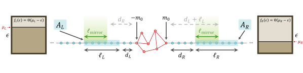
Figure 1: Schematic illustration of the model, comprised of a one-dimensional lattice that contains a generic current-conserving noninteracting impurity, and is connected at its ends to two zero-temperature reservoirs of noninteracting fermions. Sites that constitute the impurity region are marked in red, and all other sites are marked in blue. See Subsec. II.2 of the text for further details on the notations, and Eq. (11) for the definition of $\ell_{{\rm mirror}}$.

The many-body nonequilibrium steady state that we inspect originates in an occupation bias between left and right scattering states: left scattering states are occupied up to a chemical potential $\mu_{{\scriptscriptstyle L}}$, and right scattering states are occupied up to a chemical potential $\mu_{{\scriptscriptstyle R}}$, with $\mu_{{\scriptscriptstyle L}}\neq\mu_{{\scriptscriptstyle R}}$. We can define corresponding Fermi momenta through $k_{{\scriptscriptstyle F,i}}=\cos^{-1}\!\left(-\mu_{i}/2\eta\right)$ (for $i=L,R$), such that the many-body state is in essence a tilted Fermi sea. This steady state can be thought of as the result of connecting the chain to two edge reservoirs containing free fermions at zero temperature and with the chemical potentials $\mu_{{\scriptscriptstyle L}}$ and $\mu_{{\scriptscriptstyle R}}$ (such that, in each reservoir, single-particle energy states are occupied with probability $f_{i}\!\left(\epsilon\right)=\Theta\!\left(\mu_{i}-\epsilon\right)$ as a function of the energy $\epsilon$, with $\Theta$ being the Heaviside step function), and subsequently going to the thermodynamic limit of an infinite chain; such a scenario is depicted in Fig. 1. Alternatively, the steady state can be seen as the long-time limit following a quench where two zero-temperature Fermi seas with the chemical potentials $\mu_{{\scriptscriptstyle L}}$ and $\mu_{{\scriptscriptstyle R}}$ are joined together at the impurity.

The most remarkable correlation properties of this nonequilibrium steady state are revealed when considering the correlations between two subsystems on opposite sides of the impurity. We specifically consider an interval $A_{{\scriptscriptstyle L}}$ to the left of the impurity, containing the sites $m$ where $-d_{{\scriptscriptstyle L}}-\ell_{{\scriptscriptstyle L}}\leq m+m_{0}\leq-d_{{\scriptscriptstyle L}}-1$, and another interval $A_{{\scriptscriptstyle R}}$ to the right of the impurity, containing the sites $m$ where $d_{{\scriptscriptstyle R}}+1\leq m-m_{0}\leq d_{{\scriptscriptstyle R}}+\ell_{{\scriptscriptstyle R}}$. For the subsystem $A_{i}$, the length scales $\ell_{i}$ and $d_{i}$ thus represent the length of the subsystem and its distance from the impurity region, respectively. An example for such a configuration is illustrated in Fig. 1. For our asymptotic calculation, we assume that these length scales are all much larger than the size of the impurity, i.e., $\ell_{i},d_{i}\gg 2m_{0}+1$. For future convenience, we let $A=A_{{\scriptscriptstyle L}}\cup A_{{\scriptscriptstyle R}}$ denote the union of the two subsystems of interest.

II.3 Recap of previous results

Here we recount the results reported in Refs. [18, 45] for entropies and correlation measures associated with subsystems $A_{{\scriptscriptstyle L}}$ and $A_{{\scriptscriptstyle R}}$. As already mentioned, the results of Ref. [45] included only the leading-order (volume-law) terms in the asymptotics of these quantities. In Appendix A we repeat a crucial technical step that was performed in Ref. [45] to obtain these results, since we rely on it again in our current derivation of the subleading corrections.

Most notably, in Ref. [45] we observed that, to a leading order, all the aforementioned quantities of interest (the MI, the negativity and their Rényi counterparts) depend on the distances $d_{{\scriptscriptstyle L}}$ and $d_{{\scriptscriptstyle R}}$ from the impurity only through their difference $d_{{\scriptscriptstyle L}}-d_{{\scriptscriptstyle R}}$. In particular, they remain the same when fixing this difference and taking the limit $d_{i}/\ell_{i}\to\infty$, revealing strong long-range correlations and entanglement in the steady state. Due to this behavior, the results of Ref. [45] are most conveniently presented if one first defines

$$\ell_{{\rm mirror}}=\max\!\left\{\min\!\left\{d_{{\scriptscriptstyle L}}+\ell_{{\scriptscriptstyle L}},d_{{\scriptscriptstyle R}}+\ell_{{\scriptscriptstyle R}}\right\}-\max\!\left\{d_{{\scriptscriptstyle L}},d_{{\scriptscriptstyle R}}\right\},0\right\},$$ (11)

which is the mirror-image overlap between subsystems $A_{{\scriptscriptstyle L}}$ and $A_{{\scriptscriptstyle R}}$: $\ell_{{\rm mirror}}$ counts the number of pairs $\left(-m,m\right)\in A_{{\scriptscriptstyle L}}\times A_{{\scriptscriptstyle R}}$; that is, the number of sites shared between the subsystems upon reflecting one of them about $m=0$ (see Fig. 1). $\ell_{{\rm mirror}}$ is conspicuously dependent on $d_{{\scriptscriptstyle L}}$ and $d_{{\scriptscriptstyle R}}$ only through $d_{{\scriptscriptstyle L}}-d_{{\scriptscriptstyle R}}$. In what follows, we will also use the notations $\Delta\ell_{i}=\ell_{i}-\ell_{{\rm mirror}}$, $k_{+}=\max\!\left\{k_{{\scriptscriptstyle F,L}},k_{{\scriptscriptstyle F,R}}\right\}$ and $k_{-}=\min\!\left\{k_{{\scriptscriptstyle F,L}},k_{{\scriptscriptstyle F,R}}\right\}$.

To be explicit, in Ref. [45] we have found that, to a leading order, the Rényi entropies of subsystems $A_{{\scriptscriptstyle L}}$, $A_{{\scriptscriptstyle R}}$ and $A$ are given by

$$S_{A_{i}}^{\left(n\right)} \sim\frac{\ell_{i}}{1-n}\int_{k_{-}}^{k_{+}}\frac{dk}{2\pi}\ln\!\left[\left({\cal T}\!\left(k\right)\right)^{n}+\left({\cal R}\!\left(k\right)\right)^{n}\right],$$

$$S_{A}^{\left(n\right)} \sim\frac{\Delta\ell_{{\scriptscriptstyle L}}+\Delta\ell_{{\scriptscriptstyle R}}}{1-n}\int_{k_{-}}^{k_{+}}\frac{dk}{2\pi}\ln\!\left[\left({\cal T}\!\left(k\right)\right)^{n}+\left({\cal R}\!\left(k\right)\right)^{n}\right].$$ (12)

This directly leads (recall Eq. (4)) to the asymptotics of the Rényi MI, namely

$${\cal I}_{A_{L}:A_{R}}^{\left(n\right)}\sim\frac{\ell_{{\rm mirror}}}{1-n}\!\int_{k_{-}}^{k_{+}}\frac{dk}{\pi}\ln\!\left[\left({\cal T}\!\left(k\right)\right)^{n}+\left({\cal R}\!\left(k\right)\right)^{n}\right],$$ (13)

and the MI is then simply obtained by taking the $n\to 1$ limit:

$${\cal I}_{A_{L}:A_{R}}\sim\ell_{{\rm mirror}}\!\int_{k_{-}}^{k_{+}}\frac{dk}{\pi}\left[-{\cal T}\!\left(k\right)\ln{\cal T}\!\left(k\right)-\!{\cal R}\!\left(k\right)\ln{\cal R}\!\left(k\right)\right].$$ (14)

Furthermore, the Rényi negativities were found to satisfy

$${\cal E}_{n} \sim\ell_{{\rm mirror}}\int_{k_{-}}^{k_{+}}\frac{dk}{\pi}\ln\!\left[\left({\cal T}\!\left(k\right)\right)^{n/2}+\left({\cal R}\!\left(k\right)\right)^{n/2}\right]+\left(\Delta\ell_{{\scriptscriptstyle L}}+\Delta\ell_{{\scriptscriptstyle R}}\right)\int_{k_{-}}^{k_{+}}\frac{dk}{2\pi}\ln\!\left[\left({\cal T}\!\left(k\right)\right)^{n}+\left({\cal R}\!\left(k\right)\right)^{n}\right],$$ (15)

which in the limit $n\to 1$ gives the behavior of the fermionic negativity:

$${\cal E}\sim\ell_{{\rm mirror}}\!\int_{k_{-}}^{k_{+}}\frac{dk}{\pi}\ln\!\left[\left({\cal T}\!\left(k\right)\right)^{1/2}+\left({\cal R}\!\left(k\right)\right)^{1/2}\right].$$ (16)

A salient attribute of Eqs. (12)–(16) is that the volume-law terms appearing in all of them identically vanish either in the absence of the bias (i.e., if $k_{{\scriptscriptstyle F,L}}=k_{{\scriptscriptstyle F,R}}$), or if ${\cal T}\!\left(k\right)\in\left\{0,1\right\}$ for all $k\in\left[k_{-},k_{+}\right]$; we refer to the latter scenario as that of a “trivial” impurity, which either perfectly transmits or perfectly reflects incoming particles. If instead both the bias and the scattering are nontrivial, then the volume-law terms in Eqs. (12)–(16) are nonzero. In other words, the voltage bias and the nontrivial scattering are necessary and sufficient conditions for observing the extensive entropies in Eq. (12) and the extensive long-range correlations captured by Eqs. (13)–(16).

Another important result on which we will rely in our analysis pertains to the subleading logarithmic terms of the Rényi entropies for a single interval $A_{i}$ in the long-range regime $d_{i}/\ell_{i}\gg 1$. In Ref. [18] we have shown that, for $d_{i}/\ell_{i}\gg 1$ and up to ${\cal O}\!\left(1\right)$ corrections, the single-interval entropies obey

$$S_{A_{L}}^{\left(n\right)} \sim\frac{\ell_{{\scriptscriptstyle L}}}{1-n}\int_{k_{-}}^{k_{+}}\frac{dk}{2\pi}\ln\!\left[\left({\cal T}\!\left(k\right)\right)^{n}+\left({\cal R}\!\left(k\right)\right)^{n}\right]+\frac{1+n}{12n}\ln\ell_{{\scriptscriptstyle L}}+\frac{\ln\ell_{{\scriptscriptstyle L}}}{1-n}\left[Q_{n}\!\left({\cal T}\!\left(k_{{\scriptscriptstyle F,L}}\right)\right)+Q_{n}\!\left({\cal R}\!\left(k_{{\scriptscriptstyle F,R}}\right)\right)\right],$$

$$S_{A_{R}}^{\left(n\right)} \sim\frac{\ell_{{\scriptscriptstyle R}}}{1-n}\int_{k_{-}}^{k_{+}}\frac{dk}{2\pi}\ln\!\left[\left({\cal T}\!\left(k\right)\right)^{n}+\left({\cal R}\!\left(k\right)\right)^{n}\right]+\frac{1+n}{12n}\ln\ell_{{\scriptscriptstyle R}}+\frac{\ln\ell_{{\scriptscriptstyle R}}}{1-n}\left[Q_{n}\!\left({\cal T}\!\left(k_{{\scriptscriptstyle F,R}}\right)\right)+Q_{n}\!\left({\cal R}\!\left(k_{{\scriptscriptstyle F,L}}\right)\right)\right],$$ (17)

where the function $Q_{n}$ is defined below, see Eq. (18).

A word of caution is in order regarding Eq. (17): its derivation assumes a finite bias ($k_{{\scriptscriptstyle F,L}}\neq k_{{\scriptscriptstyle F,R}}$), and the result for the case of no bias ($k_{{\scriptscriptstyle F,L}}=k_{{\scriptscriptstyle F,R}}$) cannot be recovered by naively taking the corresponding limit of Eq. (17). This is because the logarithmic term arises from discontinuities in the local distribution of momentum states, and in this no-bias limit two discontinuities merge into a single one (this issue comes up again in the derivation of the logarithmic corrections to $S_{A}^{\left(n\right)}$, and so we discuss it with more technical details in Subsec. IV.2.1). The proper limit of the entropies in the no-bias case is instead $S_{A_{i}}^{\left(n\right)}\sim\frac{1+n}{6n}\ln\ell_{i}$, equal to the equilibrium result for free fermions on a homogeneous tight-binding lattice [29].

II.4 Useful notations

Here we introduce several useful notations that will make the presentation of our main results more concise. For any $0\leq p\leq 1$ and any $n$, we define the function

$$Q_{n}\!\left(p\right) =\frac{n}{2\pi^{2}}\int_{p}^{1}dx\frac{x^{n-1}-\left(1-x\right)^{n-1}}{x^{n}+\left(1-x\right)^{n}}\ln\!\left(\frac{1-x}{x-p}\right)$$

$$=-\frac{n}{12}+\int_{0}^{1}\frac{dx}{2\pi^{2}x}\left\{\ln\!\left[\left(1+px\right)^{n}+\left(\left(1-p\right)x\right)^{n}\right]+\ln\!\left[\frac{\left(x+p\right)^{n}+\left(1-p\right)^{n}}{p^{n}+\left(1-p\right)^{n}}\right]\right\}.$$ (18)

This function in particular satisfies $Q_{n}\!\left(1\right)=0$ and $Q_{n}\!\left(0\right)=\frac{1}{12}\left(\frac{1}{n}-n\right)$. Additionally, for $0\leq{\cal T}\leq 1$ and ${\cal R}=1-{\cal T}$, we define

$$\widetilde{Q}_{n}\!\left({\cal T}\right) =Q_{n}\!\left({\cal T}\right)+Q_{n}\!\left({\cal R}\right)+\frac{n}{2\pi^{2}}\int_{{\cal R}}^{{\cal T}}dx\frac{x^{n-1}-\left(1-x\right)^{n-1}}{x^{n}+\left(1-x\right)^{n}}\ln\!\left|\frac{{\cal R}-x}{{\cal T}-x}\right|$$

$$=-\frac{n}{12}+\int_{0}^{1}\frac{dx}{2\pi^{2}x}\left\{\ln\!\left[\left(1+{\cal T}x\right)^{n}+\left({\cal R}x\right)^{n}\right]+\ln\!\left[\left(1+{\cal R}x\right)^{n}+\left({\cal T}x\right)^{n}\right]\right\}$$

$$+\int_{0}^{1}\frac{dx}{2\pi^{2}x}\left\{\ln\!\left[\frac{\left(x+{\cal T}\right)^{n}+{\cal R}^{n}}{\left({\cal T}+{\cal R}x\right)^{n}+\left({\cal R}+{\cal T}x\right)^{n}}\right]+\ln\!\left[\frac{\left(x+{\cal R}\right)^{n}+{\cal T}^{n}}{\left({\cal T}+{\cal R}x\right)^{n}+\left({\cal R}+{\cal T}x\right)^{n}}\right]\right\},$$ (19)

as well as the functions

$$q\!\left({\cal T}\right) =\frac{1}{24}-\int_{0}^{1}\frac{dx}{2\pi^{2}x}\cdot\frac{\left(1+{\cal R}x\right)\ln\!\left(1+{\cal R}x\right)+\left(1+{\cal T}x\right)\ln\!\left(1+{\cal T}x\right)}{1+x}$$

$$+\int_{0}^{1}\frac{dx}{2\pi^{2}x}\left[{\cal T}\ln{\cal T}+{\cal R}\ln{\cal R}-\frac{\left({\cal R}+x\right)\ln\!\left({\cal R}+x\right)+\left({\cal T}+x\right)\ln\!\left({\cal T}+x\right)}{1+x}\right],$$ (20)

and

$$\widetilde{q}\!\left({\cal T}\right)=q\!\left({\cal T}\right)+\frac{1}{12}+\int_{0}^{1}\frac{dx}{\pi^{2}x}\left[\frac{\left({\cal R}+{\cal T}x\right)\ln\!\left({\cal R}+{\cal T}x\right)+\left({\cal T}+{\cal R}x\right)\ln\!\left({\cal T}+{\cal R}x\right)}{1+x}-{\cal T}\ln{\cal T}-{\cal R}\ln{\cal R}\right].$$ (21)

The functions $q\!\left({\cal T}\right)$ and $\widetilde{q}\!\left({\cal T}\right)$ will appear in the analytical expression for the logarithmic term of the MI. To make their dependence on ${\cal T}$ more apparent, we plot them in Fig. 2, where one may observe that they both vanish for ${\cal T}=0,1$, while for $0<{\cal T}<1$ we have $q\!\left({\cal T}\right)<0$ and $\widetilde{q}\!\left({\cal T}\right)>0$.

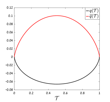
Figure 2: The functions $q\!\left({\cal T}\right)$ and $\widetilde{q}\!\left({\cal T}\right)$, given in Eqs. (20) and (21), respectively.

III Asymptotics beyond volume-law entanglement

III.1 Main results

The new results that we present in this work apply to the long-range limit: $d_{i}/\ell_{i}\to\infty$, with $d_{{\scriptscriptstyle L}}-d_{{\scriptscriptstyle R}}$ kept fixed. The volume-law asymptotics that have been previously derived (see Subsec. II.3) are independent of the absolute distances of the subsystems from the impurity, but subleading corrections are in general sensitive to these distances. We thus focus on the long-range limit so that our results capture the nature of the unique long-range correlations produced in the steady state.

Let $m_{1}\leq m_{2}\leq m_{3}\leq m_{4}$ denote the lengths $d_{{\scriptscriptstyle L}}$, $\ell_{{\scriptscriptstyle L}}+d_{{\scriptscriptstyle L}}$, $d_{{\scriptscriptstyle R}}$ and $\ell_{{\scriptscriptstyle R}}+d_{{\scriptscriptstyle R}}$ in ascending order. Our analysis shows that, in the long-range limit, the asymptotics of the Rényi MI between $A_{{\scriptscriptstyle L}}$ and $A_{{\scriptscriptstyle R}}$ is given by

$${\cal I}_{A_{L}:A_{R}}^{\left(n\right)} \sim\frac{\ell_{{\rm mirror}}}{1-n}\int_{k_{-}}^{k_{+}}\frac{dk}{\pi}\ln\!\left[\left({\cal T}\!\left(k\right)\right)^{n}+\left({\cal R}\!\left(k\right)\right)^{n}\right]$$

$$+\frac{1}{2\left(1-n\right)}\left[{\cal G}_{n}^{\left({\rm log}\right)}\!\left(k_{{\scriptscriptstyle F,L}},\ell_{{\scriptscriptstyle L}},\ell_{{\scriptscriptstyle R}},d_{{\scriptscriptstyle L}}-d_{{\scriptscriptstyle R}}\right)+{\cal G}_{n}^{\left({\rm log}\right)}\!\left(k_{{\scriptscriptstyle F,R}},\ell_{{\scriptscriptstyle L}},\ell_{{\scriptscriptstyle R}},d_{{\scriptscriptstyle L}}-d_{{\scriptscriptstyle R}}\right)\right],$$ (22)

where we defined

$${\cal G}_{n}^{\left({\rm log}\right)}\!\left(k_{{\scriptscriptstyle F}},\ell_{{\scriptscriptstyle L}},\ell_{{\scriptscriptstyle R}},d_{{\scriptscriptstyle L}}-d_{{\scriptscriptstyle R}}\right) =\left(Q_{n}\!\left({\cal T}\!\left(k_{{\scriptscriptstyle F}}\right)\right)+Q_{n}\!\left({\cal R}\!\left(k_{{\scriptscriptstyle F}}\right)\right)-\frac{1}{12}\left(\frac{1}{n}-n\right)\right)\ln\!\left|\frac{\left(m_{3}-m_{1}\right)\left(m_{4}-m_{2}\right)}{\left(\ell_{{\scriptscriptstyle L}}+d_{{\scriptscriptstyle L}}-\ell_{{\scriptscriptstyle R}}-d_{{\scriptscriptstyle R}}\right)\left(d_{{\scriptscriptstyle L}}-d_{{\scriptscriptstyle R}}\right)}\right|$$

$$+\widetilde{Q}_{n}\!\left({\cal T}\!\left(k_{{\scriptscriptstyle F}}\right)\right)\ln\!\left|\frac{\left(m_{3}-m_{1}\right)\left(m_{4}-m_{2}\right)}{\left(\ell_{{\scriptscriptstyle R}}+d_{{\scriptscriptstyle R}}-d_{{\scriptscriptstyle L}}\right)\left(\ell_{{\scriptscriptstyle L}}+d_{{\scriptscriptstyle L}}-d_{{\scriptscriptstyle R}}\right)}\right|.$$ (23)

Eq. (22) may be taken to the limit $n\to 1$ to obtain the von Neumann MI. This yields

$${\cal I}_{A_{L}:A_{R}} \sim\ell_{{\rm mirror}}\int_{k_{-}}^{k_{+}}\frac{dk}{\pi}\left[-{\cal T}\!\left(k\right)\ln{\cal T}\!\left(k\right)-{\cal R}\!\left(k\right)\ln{\cal R}\!\left(k\right)\right]$$

$$+\frac{1}{2}\left[g^{\left({\rm log}\right)}\!\left(k_{{\scriptscriptstyle F,L}},\ell_{{\scriptscriptstyle L}},\ell_{{\scriptscriptstyle R}},d_{{\scriptscriptstyle L}}-d_{{\scriptscriptstyle R}}\right)+g^{\left({\rm log}\right)}\!\left(k_{{\scriptscriptstyle F,R}},\ell_{{\scriptscriptstyle L}},\ell_{{\scriptscriptstyle R}},d_{{\scriptscriptstyle L}}-d_{{\scriptscriptstyle R}}\right)\right].$$ (24)

Here we defined the following notation to represent the contribution of each Fermi momentum to the logarithmic term of the MI:

$$g^{\left({\rm log}\right)}\!\left(k_{{\scriptscriptstyle F}},\ell_{{\scriptscriptstyle L}},\ell_{{\scriptscriptstyle R}},d_{{\scriptscriptstyle L}}-d_{{\scriptscriptstyle R}}\right) =q\!\left({\cal T}\!\left(k_{{\scriptscriptstyle F}}\right)\right)\ln\!\left|\frac{\left(m_{3}-m_{1}\right)\left(m_{4}-m_{2}\right)}{\left(\ell_{{\scriptscriptstyle L}}+d_{{\scriptscriptstyle L}}-\ell_{{\scriptscriptstyle R}}-d_{{\scriptscriptstyle R}}\right)\left(d_{{\scriptscriptstyle L}}-d_{{\scriptscriptstyle R}}\right)}\right|$$

$$+\widetilde{q}\!\left({\cal T}\!\left(k_{{\scriptscriptstyle F}}\right)\right)\ln\!\left|\frac{\left(m_{3}-m_{1}\right)\left(m_{4}-m_{2}\right)}{\left(\ell_{{\scriptscriptstyle R}}+d_{{\scriptscriptstyle R}}-d_{{\scriptscriptstyle L}}\right)\left(\ell_{{\scriptscriptstyle L}}+d_{{\scriptscriptstyle L}}-d_{{\scriptscriptstyle R}}\right)}\right|;$$ (25)

as can be seen in Eq. (24), these contributions are weighted equally. It is noteworthy that the two terms appearing in Eq. (25) have distinct signs. Suppose that $0<{\cal T}\!\left(k_{{\scriptscriptstyle F}}\right)<1$, then the first summand in Eq. (25) vanishes if $\ell_{{\rm mirror}}=0$, and is negative for $\ell_{{\rm mirror}}>0$, meaning that it decreases the correlation between $A_{{\scriptscriptstyle L}}$ and $A_{{\scriptscriptstyle R}}$ when they have nonzero mirror-image overlap. On the other hand, the second summand vanishes if either $\Delta\ell_{{\scriptscriptstyle L}}=0$ or $\Delta\ell_{{\scriptscriptstyle R}}=0$, and is positive otherwise; this implies that this term increases the correlation between $A_{{\scriptscriptstyle L}}$ and $A_{{\scriptscriptstyle R}}$ unless their mirror-image overlap is maximal (i.e., the mirror image of one of them is contained in the other).

We stress that Eqs. (22) and (24) can be applied also to degenerate cases where differences appearing inside the logarithms vanish; the apparent conundrum is solved simply by omitting the problematic difference (as will be justified by the derivation). For example, if $A_{{\scriptscriptstyle R}}$ has no overlap with the mirror image of $A_{{\scriptscriptstyle L}}$ but they exactly touch each other, such that $\ell_{{\scriptscriptstyle R}}+d_{{\scriptscriptstyle R}}=d_{{\scriptscriptstyle L}}$, then in Eq. (22) both the linear term and the first logarithmic term from Eq. (23) vanish, while in the second logarithmic term from Eq. (23) we drop the $\left(\ell_{{\scriptscriptstyle R}}+d_{{\scriptscriptstyle R}}-d_{{\scriptscriptstyle L}}\right)$ term appearing in the denominator. Eq. (22) then reads

$${\cal I}_{A_{L}:A_{R}}^{\left(n\right)} \sim\frac{\widetilde{Q}_{n}\!\left({\cal T}\!\left(k_{{\scriptscriptstyle F,L}}\right)\right)+\widetilde{Q}_{n}\!\left({\cal T}\!\left(k_{{\scriptscriptstyle F,R}}\right)\right)}{2\left(1-n\right)}\ln\!\left(\frac{\ell_{{\scriptscriptstyle L}}\ell_{{\scriptscriptstyle R}}}{\ell_{{\scriptscriptstyle L}}+\ell_{{\scriptscriptstyle R}}}\right).$$ (26)

The recipe that we will present for the calculation of the MI asymptotics can be also applied to the calculation of the fermionic negativity asymptotics, up to the logarithmic order. In Subsec. IV.3 we elaborate on how this extension of the recipe can be done in principle, though its complete execution is more cumbersome than in the case of the MI calculation. For this reason we present the full result for the negativity asymptotics only in the symmetric case with $\ell_{{\scriptscriptstyle L}}=\ell_{{\scriptscriptstyle R}}\equiv\ell$ and $d_{{\scriptscriptstyle L}}=d_{{\scriptscriptstyle R}}$ (again, the limit $d_{i}/\ell_{i}\to\infty$ is taken). The Rényi negativities are then given by

$${\cal E}_{n} \sim\ell\int_{k_{-}}^{k_{+}}\frac{dk}{\pi}\ln\!\left[\left({\cal T}\!\left(k\right)\right)^{n/2}+\left({\cal R}\!\left(k\right)\right)^{n/2}\right]-\frac{n}{4}\ln\ell$$

$$+\ln\ell\left[Q_{n/2}\!\left({\cal T}\!\left(k_{{\scriptscriptstyle F,L}}\right)\right)+Q_{n/2}\!\left({\cal R}\!\left(k_{{\scriptscriptstyle F,L}}\right)\right)+Q_{n/2}\!\left({\cal T}\!\left(k_{{\scriptscriptstyle F,R}}\right)\right)+Q_{n/2}\!\left({\cal R}\!\left(k_{{\scriptscriptstyle F,R}}\right)\right)\right],$$ (27)

and the fermionic negativity is accordingly given by their $n\to 1$ limit, namely

$${\cal E} \sim\ell\int_{k_{-}}^{k_{+}}\frac{dk}{\pi}\ln\!\left[\left({\cal T}\!\left(k\right)\right)^{1/2}+\left({\cal R}\!\left(k\right)\right)^{1/2}\right]-\frac{1}{4}\ln\ell$$

$$+\ln\ell\left[Q_{1/2}\!\left({\cal T}\!\left(k_{{\scriptscriptstyle F,L}}\right)\right)+Q_{1/2}\!\left({\cal R}\!\left(k_{{\scriptscriptstyle F,L}}\right)\right)+Q_{1/2}\!\left({\cal T}\!\left(k_{{\scriptscriptstyle F,R}}\right)\right)+Q_{1/2}\!\left({\cal R}\!\left(k_{{\scriptscriptstyle F,R}}\right)\right)\right].$$ (28)

We emphasize that the Rényi MI, the MI and the negativity all vanish either in the presence of a trivial impurity (with ${\cal T}\!\left(k\right)\in\left\{0,1\right\}$ for all $k$) or in the absence of a bias. In Subsec. II.3 we noted that this property holds for the leading-order extensive terms of these quantities, which were derived in Ref. [45]; in Subsec. IV.1 we show that it is true at all orders, since in either of the two cases the correlations between $A_{{\scriptscriptstyle L}}$ and $A_{{\scriptscriptstyle R}}$ vanish for $d_{i}/\ell_{i}\to\infty$ (the Rényi negativities do not vanish, in congruence with them not being proper correlation measures). In particular, this of course implies that the logarithmic terms in Eqs. (22), (24), and (28) should vanish in both cases. In the case of a trivial impurity this is directly seen by substituting ${\cal T}=0$ or ${\cal T}=1$ into the logarithmic terms (in Eq. (22) we use the fact that $\widetilde{Q}_{n}\!\left(1\right)=\widetilde{Q}_{n}\!\left(0\right)=0$), while these terms do not vanish if one simply substitutes $k_{{\scriptscriptstyle F,L}}=k_{{\scriptscriptstyle F,R}}$ into the equations. Like in the case of single-interval entropies, this discrepancy occurs due to non-commuting limits (see the discussion following Eq. (17)), and we point it out in order to stress that our analytical expressions rely on the assumption of a finite bias, and one could be misled by naively taking their limits to the equilibrium scenario. Since for all the quantities that we consider here the extensive term tends to zero near the no-bias limit while the logarithmic term does not, it is clear that the logarithmic term becomes especially significant when the bias is small but finite.

III.2 Comparison to numerics

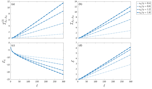
Figure 3: Scaling of (a) the 2-Rényi mutual information, (b) the mutual information, (c) the 4-Rényi negativity and (d) the fermionic negativity between subsystems $A_{{\scriptscriptstyle L}}$ and $A_{{\scriptscriptstyle R}}$ in the single-site impurity model, for a symmetric subsystem configuration with $\ell_{{\scriptscriptstyle L}}=\ell_{{\scriptscriptstyle R}}\equiv\ell$ and $d_{{\scriptscriptstyle L}}=d_{{\scriptscriptstyle R}}$. The long-range limit $d_{i}/\ell_{i}\to\infty$ is taken, and the results are plotted for various values of the impurity energy $\epsilon_{0}$, while setting the Fermi momenta at $k_{{\scriptscriptstyle F,R}}=\pi/2$ and $k_{{\scriptscriptstyle F,L}}=k_{{\scriptscriptstyle F,R}}+0.2$. In all the panels, continuous lines designate the analytical results (Eqs. (22), (24), (27) and (28), respectively; an additive constant-in-$\ell$ term constitutes the only fitting parameter), while dots represent numerical results (the computation of which is discussed in Subsec. IV.1).

In order to corroborate our asymptotic analysis, we checked the analytical results reported in Subsec. III.1 against numerical computations. The correlation measures discussed in this paper can be computed numerically through exact diagonalization of two-point correlation matrices, as further explained in Subsec. IV.1; there we also provide the explicit expression for the two-point correlation function in the limit $d_{i}/\ell_{i}\to\infty$ (see Eq. (37)).

As a specific example for a noninteracting impurity, we choose a single-site impurity with a nonzero on-site energy. That is, in the Hamiltonian of Eq. (7) we set $m_{0}=0$ and ${\cal H}_{{\rm scat}}=\epsilon_{0}c_{0}^{\dagger}c_{0}$, with $\epsilon_{0}$ being the impurity energy. The corresponding transmission probability is given by

$${\cal T}\!\left(k\right)=\frac{\sin^{2}\!k}{\sin^{2}\!k+\left(\epsilon_{0}/2\eta\right)^{2}}.$$ (29)

In Fig. 3 we show a comparison between our analytical results and numerics, for the symmetric configuration where the two subsystems of interest are of equal length and within an equal distance from the impurity. We plot the scaling with subsystem length of the MI, negativity, 2-Rényi MI and 4-Rényi negativity, where the analytical results include the exact expressions for the linear and logarithmic terms, along with an additive constant correction constituting the only fitting parameter. The excellent agreement of our results with the numerics is clearly evident.

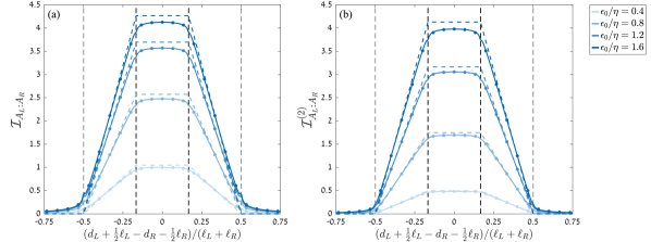
Figure 4: (a) Scaling of the mutual information between subsystems $A_{{\scriptscriptstyle L}}$ and $A_{{\scriptscriptstyle R}}$ in the single-site impurity model, for fixed subsystem lengths ($\ell_{{\scriptscriptstyle L}}=100$ and $\ell_{{\scriptscriptstyle R}}=200$) and varying $d_{{\scriptscriptstyle L}}-d_{{\scriptscriptstyle R}}$. The long-range limit $d_{i}/\ell_{i}\to\infty$ is taken, and the results are plotted for various values of the impurity energy $\epsilon_{0}$, while setting the Fermi momenta at $k_{{\scriptscriptstyle F,R}}=\pi/2$ and $k_{{\scriptscriptstyle F,L}}=k_{{\scriptscriptstyle F,R}}+0.2$. Continuous lines represent the analytical result of Eq. (24), dashed blue lines represent the analytical result including only the leading-order volume-law term, and dots represent the numerical results (the computation of which is discussed in Subsec. IV.1). Employing the notation $\bar{A}_{{\scriptscriptstyle L}}=\left\{m|-\!m\in A_{{\scriptscriptstyle L}}\right\}$ for the mirror image of $A_{{\scriptscriptstyle L}}$, black dashed vertical lines designate the range of values of $d_{{\scriptscriptstyle L}}-d_{{\scriptscriptstyle R}}$ in which $\bar{A}_{{\scriptscriptstyle L}}\subset A_{{\scriptscriptstyle R}}$, while gray dashed vertical lines mark the range in which $\bar{A}_{{\scriptscriptstyle L}}\cap A_{{\scriptscriptstyle R}}\neq\phi$. Panel (b) shows a similar analysis for the 2-Rényi mutual information, where the analytical results were computed using Eq. (22).

This importance of the logarithmic correction, which is the refinement provided by the current work relative to the results reported in Ref. [45], becomes especially conspicuous when we compare the analytical results and the numerics for a scenario where we fix the lengths of the two subsystems and vary the position of one of them. In Fig. 4 we plot for such a scenario the 2-Rényi MI and the MI, for which we explicitly derived the logarithmic terms for a general subsystem configuration, given in Eqs. (22) and (24), respectively. As expected from the form of the leading-order terms appearing in Eqs. (22) and (24), these measures reach a maximal value for a maximal mirror-image overlap between the two subsystems. However, the corrections beyond the leading order are clearly substantial: by plotting the results of Eqs. (22) and (24) both with the logarithmic terms and without them, we observe that their inclusion leads to a much more accurate agreement with the numerics.

Finally, we should also emphasize that the derivation of the logarithmic terms in Eqs. (22) and (24) relies on the study of a simplified version of the nonequilibrium steady state, where the scattering matrix associated with the impurity is assumed to be independent of the energy of the incoming particle. The extension of the results to energy-dependent scattering does not rely on a direct computation, but is rather conjectural; it relies on an analogy with the exact form of the logarithmic term for a symmetric subsystem configuration, for which a direct computation is indeed possible (see more details in Subsec. IV.2). Since our choice of an impurity model gives rise to an energy-dependent transmission probability (Eq. (29)), the comparison shown in Fig. 4 is a nontrivial verification of this conjecture.

IV Derivation of the analytical results

This section describes in the detail the derivation of the results reported in Sec. III. First, in Subsec. IV.1 we discuss the two-point correlation structure of the steady state and its mathematical relations with the correlation measures of interest. Based on these relations, in Subsec. IV.2 we derive the analytical expression for the Rényi MI (given in Eq. (22)), and in Subsec. IV.3 we show how the same method can be employed for the computation of Rényi negativities.

IV.1 The correlation matrix and its long-range limit

Given a Gaussian state of the system, like the steady state considered in this work, subsystem correlation measures are fully determined by the restricted two-point correlation matrix $C_{X}$, with entries $\left(C_{X}\right)_{jm}=\left\langle c_{j}^{\dagger}c_{m}\right\rangle$ ($j,m\in X$). In particular, the Rényi entropy of any subsystem $X$ may be expressed as [68]

$$S_{X}^{\left(n\right)}=\frac{1}{1-n}{\rm Tr}\ln\!\left[\left(C_{X}\right)^{n}+\left(\mathbb{I}-C_{X}\right)^{n}\right].$$ (30)

In a similar fashion, the Rényi negativity ${\cal E}_{n}$ between two subsystems $X_{1}$ and $X_{2}$ within a Gaussian state can be generally written as [60, 63, 69]

$${\cal E}_{n}={\rm Tr}\ln\!\left[\left(C_{\Xi}\right)^{n/2}+\left(\mathbb{I}-C_{\Xi}\right)^{n/2}\right]+\frac{n}{2}{\rm Tr}\ln\!\left[\left(C_{X_{1}\cup X_{2}}\right)^{2}+\left(\mathbb{I}-C_{X_{1}\cup X_{2}}\right)^{2}\right].$$ (31)

Here $C_{\Xi}$ is a transformed correlation matrix, defined as

$$C_{\Xi}=\frac{1}{2}\left[\mathbb{I}-\left(\mathbb{I}+\Gamma_{+}\Gamma_{-}\right)^{-1}\left(\Gamma_{+}+\Gamma_{-}\right)\right],$$ (32)

with

$$\Gamma_{\pm}=\left(\begin{array}[]{cc}\pm i\mathbb{I}_{\left|X_{1}\right|}&0\\ 0&\mathbb{I}_{\left|X_{2}\right|}\end{array}\right)\left(\mathbb{I}-2C_{X_{1}\cup X_{2}}\right)\left(\begin{array}[]{cc}\pm i\mathbb{I}_{\left|X_{1}\right|}&0\\ 0&\mathbb{I}_{\left|X_{2}\right|}\end{array}\right),$$ (33)

assuming the entries of $C_{X_{1}\cup X_{2}}$ are ordered such that its first $\left|X_{1}\right|$ indices ($\left|X_{i}\right|$ being the size of $X_{i}$) correspond to the sites of $X_{1}$. In Ref. [45] we showed that Eq. (31) is in fact equivalent to

$${\cal E}_{n}={\rm Tr}\ln\!\left[\prod_{\gamma=-\frac{n-1}{2}}^{\frac{n-1}{2}}\left(\mathbb{I}-C_{\gamma}\right)\right],$$ (34)

with $C_{\gamma}$ defined for $\gamma=-\frac{n-1}{2},-\frac{n-3}{2},\ldots,\frac{n-1}{2}$ as

$$C_{\gamma}=\left(\begin{array}[]{cc}\left(1-e^{\frac{2\pi i\gamma}{n}}\right)\mathbb{I}_{\left|X_{1}\right|}&0\\ 0&\left(1+e^{\frac{-2\pi i\gamma}{n}}\right)\mathbb{I}_{\left|X_{2}\right|}\end{array}\right)C_{X_{1}\cup X_{2}}.$$ (35)

Eqs. (30), (31) and (34) are general formulae (applicable to any Gaussian state) that constitute the basis for the computation of all analytical and numerical results reported in this paper.

For the particular state considered in this paper, the two-point correlation function for sites $j,m$ outside the scattering region (such that $\left|j\right|,\left|m\right|>m_{0}$) can be extracted from the relation

$$\left\langle c_{j}^{\dagger}c_{m}\right\rangle=\int_{-k_{F,R}}^{k_{F,L}}\frac{{\rm d}k}{2\pi}\,\left\langle k|j\right\rangle\left\langle m|k\right\rangle,$$ (36)

using the scattering state wavefunctions given in Eqs. (8)–(9). In Ref. [45] we observed that in the long-range limit where $d_{i}/\ell_{i}\to\infty$ with $d_{{\scriptscriptstyle L}}-d_{{\scriptscriptstyle R}}$ kept fixed, the explicit expression for the correlation function in Eq. (36) is simplified, as certain contributions vanish in this limit. Accordingly, for $d_{i}/\ell_{i}\gg 1$ we may use the approximation

$$\left\langle c_{j}^{\dagger}c_{m}\right\rangle\approx\begin{cases}\int_{-k_{F,R}}^{k_{F,R}}\frac{dk}{2\pi}\,e^{-i\left(j-m\right)k}+\int_{k_{F,R}}^{k_{F,L}}\frac{dk}{2\pi}\,{\cal T}\!\left(k\right)e^{-i\left(j-m\right)k}&j,m\in A_{{\scriptscriptstyle R}},\\ \int_{-k_{F,L}}^{k_{F,L}}\frac{dk}{2\pi}\,e^{-i\left(j-m\right)k}+\int_{k_{F,L}}^{k_{F,R}}\frac{dk}{2\pi}\,{\cal T}\!\left(k\right)e^{i\left(j-m\right)k}&j,m\in A_{{\scriptscriptstyle L}},\\ \int_{k_{F,R}}^{k_{F,L}}\frac{dk}{2\pi}\,t_{{\scriptscriptstyle L}}^{*}\!\left(k\right)r_{{\scriptscriptstyle L}}\!\left(k\right)e^{-i\left(j+m\right)k}&m\in A_{{\scriptscriptstyle L}}\text{ and }j\in A_{{\scriptscriptstyle R}},\\ \int_{k_{F,L}}^{k_{F,R}}\frac{dk}{2\pi}\,t_{{\scriptscriptstyle R}}^{*}\!\left(k\right)r_{{\scriptscriptstyle R}}\!\left(k\right)e^{i\left(j+m\right)k}&j\in A_{{\scriptscriptstyle L}}\text{ and }m\in A_{{\scriptscriptstyle R}}.\end{cases}$$ (37)

Since the long-range limit is the focus of this paper, Eq. (37) was the expression used for the correlation matrix entries when numerical results were computed using Eqs. (30)–(31). As we explain in detail in the following subsections, Eq. (37) was also used as the starting point for some parts of the analytical derivation, whereas in other parts the long-range limit was taken only in a later stage of the calculation.

We may point out that Eq. (37) entails that, in the long-range limit, the two-point correlation function between a site in $A_{{\scriptscriptstyle L}}$ and another in $A_{{\scriptscriptstyle R}}$ vanishes either when the impurity is trivial or when $k_{{\scriptscriptstyle F,L}}=k_{{\scriptscriptstyle F,R}}$. Then, it is straightforward to see through Eqs. (30) and (31) that in either of these two cases the Rényi MI vanishes identically and the Rényi negativity satisfies ${\cal E}_{n}=\left(1-n\right)S_{A}^{\left(n\right)}$, meaning that both the (von Neumann) MI and the negativity vanish.

IV.2 Derivation of the mutual information asymptotics

In this subsection we discuss the derivation of Eq. (22), which reports the asymptotics of the Rényi MI in the long-range limit. As $S_{A_{L}}^{\left(n\right)}$ and $S_{A_{R}}^{\left(n\right)}$ are known exactly up to the logarithmic order from Ref. [18] (recall Eq. (17)), what remains to be done is the computation of $S_{A}^{\left(n\right)}$, the Rényi entropy of the union of the two intervals. First, in Subec. IV.2.1, we perform the computation in the case where the two intervals are of equal length, $\ell_{{\scriptscriptstyle L}}=\ell_{{\scriptscriptstyle R}}$, a choice which allows to treat the problem exactly for certain regimes of the value of $\left|d_{{\scriptscriptstyle L}}-d_{{\scriptscriptstyle R}}\right|$. Then, in the remainder of this subsection, we tackle the more general calculation (including $\ell_{{\scriptscriptstyle L}}\neq\ell_{{\scriptscriptstyle R}}$, and for any choice of $d_{{\scriptscriptstyle L}}-d_{{\scriptscriptstyle R}}$) by studying a simplified version of the steady state, and by relying on insights obtained from the exact solution featured in Subsec. IV.2.1.

IV.2.1 Special case: Equal-length intervals

We thus begin by focusing on the case where $A_{{\scriptscriptstyle L}}$ and $A_{{\scriptscriptstyle R}}$ are of equal length, $\ell_{{\scriptscriptstyle L}}=\ell_{{\scriptscriptstyle R}}\equiv\ell$. The restricted two-point correlation matrix $C_{A}$ can then be written in terms of $2\times 2$ blocks,

$$\Phi_{jm}=\left(\begin{array}[]{cc}\left\langle c_{m_{0}+d_{R}+j}^{\dagger}c_{m_{0}+d_{R}+m}\right\rangle&\left\langle c_{m_{0}+d_{R}+j}^{\dagger}c_{-m_{0}-d_{L}-m}\right\rangle\\ \left\langle c_{-m_{0}-d_{L}-j}^{\dagger}c_{m_{0}+d_{R}+m}\right\rangle&\left\langle c_{-m_{0}-d_{L}-j}^{\dagger}c_{-m_{0}-d_{L}-m}\right\rangle\end{array}\right),$$ (38)

such that $\left(C_{A}\right)_{2j-2+\sigma_{1},2m-2+\sigma_{2}}=\left(\Phi_{jm}\right)_{\sigma_{1}\sigma_{2}}$ for $\sigma_{1},\sigma_{2}\in\left\{1,2\right\}$. Substituting the long-range approximation from Eq. (37), we have a block-Toeplitz structure of $C_{A}$, meaning that the entries of the blocks $\Phi_{jm}$ depend on $j,m$ only through $j-m$. In particular, we may define a $2\times 2$ block-symbol $\Phi\!\left(k\right)$ such that

$$\Phi_{jm}\approx\int_{-\pi}^{\pi}\frac{dk}{2\pi}\Phi\!\left(k\right)e^{-i\left(j-m\right)k}.$$ (39)

The block-symbol $\Phi\!\left(k\right)$ has four discontinuity points at $k=\pm k_{{\scriptscriptstyle F,L}}$ and $k=\pm k_{{\scriptscriptstyle F,R}}$, and has a different form depending on whether $k_{{\scriptscriptstyle F,L}}>k_{{\scriptscriptstyle F,R}}$ or $k_{{\scriptscriptstyle F,L}}<k_{{\scriptscriptstyle F,R}}$; we analyze the former case for concreteness, and subsequently mention how the results of the different steps are changed in the latter case. For $k_{{\scriptscriptstyle F,L}}>k_{{\scriptscriptstyle F,R}}$, the entries of $\Phi\!\left(k\right)$ are given by

$$\Phi_{11}\!\left(k\right) =\begin{cases}1&-k_{{\scriptscriptstyle F,R}}<k<k_{{\scriptscriptstyle F,R}},\\ {\cal T}\!\left(k\right)&k_{{\scriptscriptstyle F,R}}<k<k_{{\scriptscriptstyle F,L}},\\ 0&\text{otherwise},\end{cases}$$

$$\Phi_{22}\!\left(k\right) =\begin{cases}1&-k_{{\scriptscriptstyle F,L}}<k<k_{{\scriptscriptstyle F,R}},\\ {\cal R}\!\left(k\right)&k_{{\scriptscriptstyle F,R}}<k<k_{{\scriptscriptstyle F,L}},\\ 0&\text{otherwise},\end{cases}$$

$$\Phi_{12}\!\left(k\right) =\begin{cases}t_{{\scriptscriptstyle L}}^{*}\!\left(k\right)r_{{\scriptscriptstyle L}}\!\left(k\right)e^{i\left(d_{L}-d_{R}\right)k}&k_{{\scriptscriptstyle F,R}}<k<k_{{\scriptscriptstyle F,L}},\\ 0&\text{otherwise},\end{cases}$$ (40)

and $\Phi_{21}\!\left(k\right)=\Phi_{12}\!\left(k\right)^{*}$.

Following the customary method [50], we write Rényi entropies in terms of contour integrals, using the notation $D_{\ell}\!\left(\lambda\right)=\det\!\left(\lambda\mathbb{I}_{2\ell}-C_{A}\right)$:

$$S_{A}^{\left(n\right)}=\frac{1}{\left(1-n\right)2\pi i}\lim_{\varepsilon,\delta\to 0^{+}}\int_{c\left(\varepsilon,\delta\right)}d\lambda\ln\left[\left(\lambda+\varepsilon\right)^{n}+\left(1+\varepsilon-\lambda\right)^{n}\right]\frac{d}{d\lambda}\ln D_{\ell}\!\left(\lambda\right).$$ (41)

Here $c\left(\varepsilon,\delta\right)$ is a closed contour that encircles the segment $\left[0,1\right]$ (which contains all the zeros of $D_{\ell}\!\left(\lambda\right)$), converges to this segment as $\varepsilon,\delta\to 0^{+}$, and avoids the singularities of $\ln\!\left[\left(\lambda+\varepsilon\right)^{n}+\left(1+\varepsilon-\lambda\right)^{n}\right]$ (cf. Ref. [18]). Observing that $\lambda\mathbb{I}_{2\ell}-C_{A}$ is also a block-Toeplitz matrix (with respect to the block-symbol $\lambda\mathbb{I}_{2}-\Phi\!\left(k\right)$), we use the result of the generalized Fisher-Hartwig conjecture for the large-$\ell$ asymptotics of $\ln D_{\ell}\!\left(\lambda\right)$ [70, 71]:

$$\ln D_{\ell}\!\left(\lambda\right)\sim\ell\int_{-\pi}^{\pi}\frac{dk}{2\pi}\ln\det\!\left(\lambda\mathbb{I}_{2}-\Phi\!\left(k\right)\right)+\frac{\ln\ell}{4\pi^{2}}\sum_{r}{\rm Tr}\left[\ln^{2}\!\left[\left(\lambda\mathbb{I}_{2}-\Phi\!\left(k_{r}^{-}\right)\right)\left(\lambda\mathbb{I}_{2}-\Phi\!\left(k_{r}^{+}\right)\right)^{-1}\right]\right]+\ldots,$$ (42)

where $k_{r}$ are the discontinuity points of $\Phi\!\left(k\right)$, and where the ellipsis stands for a subleading constant term, along with additional terms that vanish for $\ell\to\infty$. This then yields

$$\ln D_{\ell}\!\left(\lambda\right) \sim\left[\frac{k_{{\scriptscriptstyle F,R}}}{\pi}\ln\left(\lambda-1\right)^{2}+\frac{k_{{\scriptscriptstyle F,L}}-k_{{\scriptscriptstyle F,R}}}{\pi}\ln\lambda\left(\lambda-1\right)+\frac{\pi-k_{{\scriptscriptstyle F,L}}}{\pi}\ln\lambda^{2}\right]\ell+\frac{1}{\pi^{2}}\left(\ln\frac{\lambda-1}{\lambda}\right)^{2}\ln\ell.$$ (43)

For $k_{{\scriptscriptstyle F,L}}<k_{{\scriptscriptstyle F,R}}$ we get the same asymptotics of Eq. (43) up to the replacement $L\leftrightarrow R$.

Crucially, the use of the Fisher-Hartwig asymptotic formula implicitly assumes that $\ell$ is the largest length scale other than those already taken to infinity. In particular, Eq. (43) is valid only in the regime where $\ell\gg\left|d_{{\scriptscriptstyle L}}-d_{{\scriptscriptstyle R}}\right|$; in other words, it applies solely to a symmetric configuration of the intervals, such that they have both equal length and (approximately) equal distance from the impurity. We can also examine the opposite case $\ell\ll\left|d_{{\scriptscriptstyle L}}-d_{{\scriptscriptstyle R}}\right|$ by taking this limit in the block-Toeplitz matrix before invoking the asymptotic formula for its determinant; this simply amounts to setting $\Phi_{12}\left(k\right)=0$ for all $k$ in Eq. (40). For $k_{{\scriptscriptstyle F,L}}>k_{{\scriptscriptstyle F,R}}$, the asymptotics of the block-Toeplitz determinant is then

$$\ln D_{\ell}\!\left(\lambda\right) \sim\ell\left[\frac{k_{{\scriptscriptstyle F,R}}}{\pi}\ln\left(\lambda-1\right)^{2}+\frac{k_{{\scriptscriptstyle F,L}}-k_{{\scriptscriptstyle F,R}}}{2\pi}\ln\lambda\left(\lambda-1\right)+\int_{k_{F,R}}^{k_{F,L}}\frac{dk}{2\pi}\ln\!\left[\left(\lambda-{\cal T}\!\left(k\right)\right)\left(\lambda-{\cal R}\!\left(k\right)\right)\right]+\frac{\pi-k_{{\scriptscriptstyle F,L}}}{\pi}\ln\lambda^{2}\right]$$

$$+\frac{\ln\ell}{2\pi^{2}}\left(\ln\frac{\lambda-1}{\lambda}\right)^{2}$$

$$+\frac{\ln\ell}{4\pi^{2}}\left[\left(\ln\frac{\lambda}{\lambda-{\cal T}\!\left(k_{{\scriptscriptstyle F,L}}\right)}\right)^{2}+\left(\ln\frac{\lambda}{\lambda-{\cal R}\!\left(k_{{\scriptscriptstyle F,L}}\right)}\right)^{2}+\left(\ln\frac{\lambda-1}{\lambda-{\cal T}\!\left(k_{{\scriptscriptstyle F,R}}\right)}\right)^{2}+\left(\ln\frac{\lambda-1}{\lambda-{\cal R}\!\left(k_{{\scriptscriptstyle F,R}}\right)}\right)^{2}\right],$$ (44)

where again the result for $k_{{\scriptscriptstyle F,L}}<k_{{\scriptscriptstyle F,R}}$ is the same up to the exchange $L\leftrightarrow R$.

Substituting Eq. (43) into Eq. (41), we observe that for $\ell\gg\left|d_{{\scriptscriptstyle L}}-d_{{\scriptscriptstyle R}}\right|$ the linear term of $S_{A}^{\left(n\right)}$ vanishes, so that the leading asymptotics is given by

$$S_{A}^{\left(n\right)} \sim\frac{4}{1-n}Q_{n}\!\left(0\right)\ln\ell=\frac{1+n}{3n}\ln\ell.$$ (45)

Interestingly, this is precisely the value $S_{A}^{\left(n\right)}$ would acquire in the absence of a scatterer, i.e., in a homogeneous system of free fermions [72]. In this symmetric configuration, the effect of the scatterer on the entanglement of $A$ with its complement is thus completely eliminated. This is suggestive of the existence of a certain procedure – whereby a “folding” transformation about the location of the impurity joins together mirroring sites [43] – that could be used more generally to simplify the entanglement structure of similar steady states. In contrast, for $\ell\ll\left|d_{{\scriptscriptstyle L}}-d_{{\scriptscriptstyle R}}\right|$ the Rényi entropies are given by

$$S_{A}^{\left(n\right)} \sim\frac{\ell}{1-n}\int_{k_{-}}^{k_{+}}\frac{dk}{\pi}\ln\left[\left({\cal T}\!\left(k\right)\right)^{n}+\left({\cal R}\!\left(k\right)\right)^{n}\right]+\frac{1+n}{6n}\ln\ell$$

$$+\frac{\ln\ell}{1-n}\left[Q_{n}\!\left({\cal T}\!\left(k_{{\scriptscriptstyle F,L}}\right)\right)+Q_{n}\!\left({\cal R}\!\left(k_{{\scriptscriptstyle F,L}}\right)\right)+Q_{n}\!\left({\cal T}\!\left(k_{{\scriptscriptstyle F,R}}\right)\right)+Q_{n}\!\left({\cal R}\!\left(k_{{\scriptscriptstyle F,R}}\right)\right)\right],$$ (46)

as obtained from substituting Eq. (44) into Eq. (41).

We conclude that for $\ell_{{\scriptscriptstyle L}}=\ell_{{\scriptscriptstyle R}}\equiv\ell$, and up to a logarithmic order,

$$S_{A}^{\left(n\right)}=\begin{cases}\frac{1+n}{3n}\ln\ell&\ell\gg\left|d_{{\scriptscriptstyle L}}-d_{{\scriptscriptstyle R}}\right|,\\ S_{A_{L}}^{\left(n\right)}+S_{A_{R}}^{\left(n\right)}&\ell\ll\left|d_{{\scriptscriptstyle L}}-d_{{\scriptscriptstyle R}}\right|,\end{cases}$$ (47)

where we used the single-interval results from Eq. (17). Thus, for $\ell\gg\left|d_{{\scriptscriptstyle L}}-d_{{\scriptscriptstyle R}}\right|$ we find that the Rényi MI scales as

$${\cal I}_{A_{L}:A_{R}}^{\left(n\right)} \sim\frac{\ell}{1-n}\int_{k_{-}}^{k_{+}}\frac{dk}{\pi}\ln\left[\left({\cal T}\!\left(k\right)\right)^{n}+\left({\cal R}\!\left(k\right)\right)^{n}\right]-\frac{1+n}{6n}\ln\ell$$

$$+\frac{\ln\ell}{1-n}\left[Q_{n}\!\left({\cal T}\!\left(k_{{\scriptscriptstyle F,L}}\right)\right)+Q_{n}\!\left({\cal R}\!\left(k_{{\scriptscriptstyle F,L}}\right)\right)+Q_{n}\!\left({\cal T}\!\left(k_{{\scriptscriptstyle F,R}}\right)\right)+Q_{n}\!\left({\cal R}\!\left(k_{{\scriptscriptstyle F,R}}\right)\right)\right],$$ (48)

while for $\ell\ll\left|d_{{\scriptscriptstyle L}}-d_{{\scriptscriptstyle R}}\right|$ the Rényi MI obeys an area-law scaling with $\ell$.

In Subsec. III.1 we emphasized that our analysis relies on the assumption that $k_{{\scriptscriptstyle F,L}}\neq k_{{\scriptscriptstyle F,R}}$, meaning that the analytical expressions for the logarithmic terms of correlation measures cannot be naively taken to the no-bias limit. This is true in particular for Eq. (48), and it is instructive to explain why a simple substitution of $k_{{\scriptscriptstyle F,L}}=k_{{\scriptscriptstyle F,R}}$ fails in this case (i.e., why the limits do not commute). Indeed, when $k_{{\scriptscriptstyle F,L}}=k_{{\scriptscriptstyle F,R}}$ the analysis of the Fisher-Hartwig asymptotics of $\ln D_{\ell}\!\left(\lambda\right)$ must be modified, since instead of the four discontinuity points that the block-Toeplitz symbol in Eq. (40) has in the presence of a bias, in the absence of a bias it has only two discontinuity points. Furthermore, the symbol becomes independent of the scattering matrix and of $d_{{\scriptscriptstyle L}}-d_{{\scriptscriptstyle R}}$. It is straightforward to check that the asymptotics of the determinant $\ln D_{\ell}\!\left(\lambda\right)$ is then equal to that appearing in Eq. (43) when $k_{{\scriptscriptstyle F,L}}=k_{{\scriptscriptstyle F,R}}$ is substituted into the equation. Therefore, Eq. (45) captures the Rényi entropy of $A$ (regardless of the value of $\left|d_{{\scriptscriptstyle L}}-d_{{\scriptscriptstyle R}}\right|$). Combined with the fact that the entropy of each interval is given by $S_{A_{i}}^{\left(n\right)}\sim\frac{1+n}{6n}\ln\ell$ (as was already mentioned below Eq. (17)), we conclude that for $k_{{\scriptscriptstyle F,L}}=k_{{\scriptscriptstyle F,R}}$ both the linear term and the logarithmic term of the Rényi MI vanish; this agrees with our observation from Subsec. IV.1, which stated that, in the absence of a bias, the Rényi MI must vanish identically (in the long-range limit).

IV.2.2 Simplified steady state for the general case

We now turn to treat the more general configuration where $\ell_{{\scriptscriptstyle L}}$ and $\ell_{{\scriptscriptstyle R}}$ are not necessarily equal and with an arbitrary value of $d_{{\scriptscriptstyle L}}-d_{{\scriptscriptstyle R}}$ (but still in the long-range limit $d_{i}/\ell_{i}\to\infty$). As before, we compute Rényi entropies using their relation to the restricted correlation matrix of the subsystem of interest, given in Eq. (30). Through a series expansion, this relation can be expressed as

$$S_{X}^{\left(n\right)}=\frac{1}{1-n}\sum_{s=1}^{\infty}\frac{\left(-1\right)^{s+1}}{s}{\rm Tr}\!\left[\left\{\left(C_{X}\right)^{n}+\left(\mathbb{I}-C_{X}\right)^{n}-\mathbb{I}\right\}^{s}\right].$$ (49)

Thus, it suffices to find a systematic way to compute correlation matrix moments of the form ${\rm Tr}\!\left[\left(C_{X}\right)^{p}\right]$ (for any integer $p$), provided that the result allows to then sum up the series expansion of Eq. (49). Indeed, this was the basis for the analytical calculation we reported in Ref. [45] for the leading-order asymptotics. Yet in order to produce the logarithmic corrections, we must replace the steady state we described with a simplified version of it, from which we can nevertheless read off the entanglement structure of the original steady state.

The construction of the artificial simplified steady state is done through two assumptions. We first assume that particles emerge only from the reservoir with the higher chemical potential and occupy only the single-particle eigenstates associated with the momenta $k_{-}\leq\left|k\right|\leq k_{+}$ (i.e., the states with $\left|k\right|<k_{-}$ are taken to be empty). Our results for the Rényi MI in Eqs. (13) and (48) indeed lead to the realization that, up to the linear and logarithmic order, the correlations between $A_{{\scriptscriptstyle L}}$ and $A_{{\scriptscriptstyle R}}$ are generated solely by particles occupying the eigenstates corresponding to $k_{-}\leq\left|k\right|\leq k_{+}$, motivating the assumption that this artificial state has the same entanglement structure as the true state. It should be noted that the values of $S_{A_{i}}^{\left(n\right)}$ to which this artificial steady state gives rise disagree at the logarithmic order with the same quantities as computed for the true steady state (as they appear in Eq. (17)); yet the result for $S_{A_{L}}^{\left(n\right)}+S_{A_{R}}^{\left(n\right)}$ is the same for the two states, and this is indeed the relevant quantity for the MI calculation. The second assumption that we impose states that the scattering amplitudes in Eq. (10) are $k$-independent; this will be amended later by an appropriate insertion of the $k$-dependence into the final result that we derive.

IV.2.3 Expressing entropies with Toeplitz determinants

We continue by leveraging the simplicity of the artificial steady state to obtain useful formulae for the Rényi entropies of $A_{{\scriptscriptstyle L}}$, $A_{{\scriptscriptstyle R}}$ and $A$, which will later produce the Rényi MI asymptotics. Even though in the case of $A_{{\scriptscriptstyle L}}$ and $A_{{\scriptscriptstyle R}}$ the asymptotics of the entropies are already known from Ref. [18], we include them in the analysis as well. This is because it will turn out that treating directly the Rényi MI rather than the different entropies comprising it is somewhat simpler, due to terms that are canceled out when these entropies are combined. For concreteness, we present the following analysis focusing on the case $k_{{\scriptscriptstyle F,L}}>k_{{\scriptscriptstyle F,R}}$.

In Appendix A we explain how the simplified definition in Subsec. IV.2.2 of the steady state leads, via a stationary phase approximation [73], to the following approximation of the correlation matrix moments:

$${\rm Tr}\!\left[\left(C_{X}\right)^{p}\right]\approx\int_{\left[k_{F,R},k_{F,L}\right]^{p}}\frac{d^{p}k}{\left(2\pi\right)^{p}}\prod_{j=1}^{p}\left\{\sum_{m\in X_{L}}\left[e^{im\left(k_{j-1}-k_{j}\right)}+{\cal R}e^{im\left(k_{j}-k_{j-1}\right)}\right]+\sum_{m\in X_{R}}{\cal T}e^{im\left(k_{j-1}-k_{j}\right)}\right\}.$$ (50)

Here we define $k_{0}=k_{p}$, and we see each subsystem of interest $X$ as comprised of two disjoint components – $X_{{\scriptscriptstyle L}}$ to the left of the impurity and $X_{{\scriptscriptstyle R}}$ to its right – each being contiguous; if $X=A_{{\scriptscriptstyle L}}$ or $X=A_{{\scriptscriptstyle R}}$ then one of these components is trivial. If we discretize the integral in Eq. (50) by dividing the interval $\left[k_{{\scriptscriptstyle F,R}},k_{{\scriptscriptstyle F,L}}\right]$ into $M\gg 1$ equal-length smaller intervals, we obtain

$${\rm Tr}\!\left[\left(C_{X}\right)^{p}\right]\approx\left(\frac{\Delta k}{2\pi M}\right)^{p}\sum_{s_{1},\ldots,s_{p}=1}^{M}\prod_{j=1}^{p}\left\{\sum_{m\in X_{L}}\left[e^{im\left(k_{s_{j-1}}-k_{s_{j}}\right)}+{\cal R}e^{im\left(k_{s_{j}}-k_{s_{j-1}}\right)}\right]+\sum_{m\in X_{R}}{\cal T}e^{im\left(k_{s_{j-1}}-k_{s_{j}}\right)}\right\},$$ (51)

where $\Delta k=k_{{\scriptscriptstyle F,L}}-k_{{\scriptscriptstyle F,R}}$ and $k_{s}=k_{{\scriptscriptstyle F,R}}+\frac{\Delta k}{M}s$. This is merely an approximation of the integral as a Riemann sum, yet it constitutes a crucial step in the way to our desired solution. We observe that Eq. (51) is equivalent to writing

$${\rm Tr}\left[\left(C_{X}\right)^{p}\right]\approx\left(\frac{\Delta k}{2\pi M}\right)^{p}{\rm Tr}\left[\left(\widehat{K}^{\left(X\right)}\right)^{p}\right],$$ (52)

with $\widehat{K}^{\left(X\right)}$ being a $M\times M$ Toeplitz matrix, defined by

$$\left(\widehat{K}^{\left(X\right)}\right)_{ss^{\prime}}=\sum_{m\in X_{L}}\left[e^{-im\Delta k\left(s-s^{\prime}\right)/M}+{\cal R}e^{im\Delta k\left(s-s^{\prime}\right)/M}\right]+\sum_{m\in X_{R}}{\cal T}e^{-im\Delta k\left(s-s^{\prime}\right)/M}.$$ (53)

Then, by plugging this approximation into Eq. (49) and summing the series, we find that

$$S_{X}^{\left(n\right)}\approx\frac{1}{1-n}{\rm Tr}\ln\!\left[\left(\frac{\Delta k}{2\pi M}\widehat{K}^{\left(X\right)}\right)^{n}+\left(\mathbb{I}-\frac{\Delta k}{2\pi M}\widehat{K}^{\left(X\right)}\right)^{n}\right].$$ (54)

To complete this part, we introduce the following notation for any integer $n\geq 2$:

$$\left(z_{\gamma}\right)^{-1}=1-e^{2\pi i\gamma/n},\,\,\,\,\,\gamma=-\frac{n-1}{2},-\frac{n-3}{2},\ldots,\frac{n-1}{2}.$$ (55)

Note that if $n$ is odd then one of the possible values of $\gamma$ is $\gamma=0$, so that $\left(z_{\gamma=0}\right)^{-1}=0$. The points $z_{\gamma}$ are the roots of the polynomial

$$p_{n}\!\left(z\right)=z^{n}+\left(1-z\right)^{n}=\prod_{\gamma=-\frac{n-1}{2}}^{\frac{n-1}{2}}\left(1-\frac{z}{z_{\gamma}}\right).$$ (56)

For an even $n$, $p_{n}$ has $n$ different roots, while for an odd $n$, $p_{n}$ is of degree $n-1$ and has only $n-1$ different roots, with $\gamma=0$ designating the missing root. This decomposition of the polynomial $p_{n}$ allows us to write

$$S_{X}^{\left(n\right)}\approx\frac{1}{1-n}\sum_{\gamma=-\frac{n-1}{2}}^{\frac{n-1}{2}}\ln{\cal Z}_{\gamma}^{\left(X\right)},$$ (57)

where each ${\cal Z}_{\gamma}^{\left(X\right)}=\det K_{\gamma}^{\left(X\right)}$ is a Toeplitz determinant, with the corresponding Toeplitz matrix being $\left(K_{\gamma}^{\left(X\right)}\right)_{ss^{\prime}}=\delta_{ss^{\prime}}+\frac{\Delta k}{2\pi M}\left(e^{2\pi i\gamma/n}-1\right)\left(\widehat{K}^{\left(X\right)}\right)_{ss^{\prime}}$.

Eq. (57) represents a consequential step in our calculation, as it directly expresses the Rényi entropies using (logarithms of) Toeplitz determinants, the asymptotics of which are captured by the Fisher-Hartwig formula. The large parameter $M$ determining the asymptotic regime is not an intrinsic quantity related to the model or the state in question, but rather a fictitious quantity arising from our discretization of the momentum coordinates. We can therefore always choose it to be arbitrarily large, and the limit $M\to\infty$ must be eventually taken to recover the exact expressions for the entropies.

IV.2.4 Asymptotics of entropies via the Fisher-Hartwig formula

In order to make use of the Fisher-Hartwig formula for the large-$M$ asymptotics of the Toeplitz determinants appearing in Eq. (57), we must first cast the entries of the Toeplitz matrices $K_{\gamma}^{\left(X\right)}$ in the following form:

$$\left(K_{\gamma}^{\left(X\right)}\right)_{ss^{\prime}}=\int_{-\pi}^{\pi}\frac{d\theta}{2\pi}e^{-i\left(s-s^{\prime}\right)\theta}\phi_{\gamma}^{\left(X\right)}\!\left(\theta\right),$$ (58)

where the function $\phi_{\gamma}^{\left(X\right)}\!\left(\theta\right)$ is the appropriate Toeplitz symbol. For this purpose, we define for $i=L,R$ the angles

$$\theta_{i,-}=\frac{d_{i}}{M}\Delta k,\,\,\,\,\,\theta_{i,+}=\frac{d_{i}+\ell_{i}}{M}\Delta k,$$ (59)

and choose $M$ such that $\theta_{i,\pm}$ are not negligible but smaller than $\pi$ (the latter simply requires $M>d_{i}+\ell_{i}$). For $\ell_{i}\gg 1$, we can then approximate the the entries of $K_{\gamma}^{\left(X\right)}$ as integrals over $\left[-\pi,\pi\right]$, by replacing $m\Delta k/M$ in Eq. (53) with a continuous integration variable $\theta$, yielding

$$\phi_{\gamma}^{\left(X\right)}\!\left(\theta\right)\approx\begin{cases}T_{\gamma}^{\left(X\right)}\!\left(\theta\right)&-\pi\leq\theta<0,\\ {\cal T}\cdot T_{\gamma}^{\left(X\right)}\!\left(\theta\right)+{\cal R}\cdot T_{\gamma}^{\left(X\right)}\!\left(-\theta\right)&0\leq\theta<\pi,\end{cases}$$ (60)

where

$$T_{\gamma}^{\left(A_{L}\right)}\!\left(\theta\right) =\begin{cases}e^{2\pi i\gamma/n}&\theta\in\left[-\theta_{{\scriptscriptstyle L},+},-\theta_{{\scriptscriptstyle L},-}\right],\\ 1&{\rm otherwise}\,,\end{cases}$$

$$T_{\gamma}^{\left(A_{R}\right)}\!\left(\theta\right) =\begin{cases}e^{2\pi i\gamma/n}&\theta\in\left[\theta_{{\scriptscriptstyle R},-},\theta_{{\scriptscriptstyle R},+}\right],\\ 1&{\rm otherwise}\,,\end{cases}$$

$$T_{\gamma}^{\left(A\right)}\!\left(\theta\right) =\begin{cases}e^{2\pi i\gamma/n}&\theta\in\left[-\theta_{{\scriptscriptstyle L},+},-\theta_{{\scriptscriptstyle L},-}\right]\cup\left[\theta_{{\scriptscriptstyle R},-},\theta_{{\scriptscriptstyle R},+}\right],\\ 1&{\rm otherwise}\,.\end{cases}$$ (61)

The Toeplitz symbol $\phi_{\gamma}^{\left(X\right)}$ in Eq. (60) can be cast in the Fisher-Hartwig form [51], namely $\phi_{\gamma}^{\left(X\right)}\!\left(\theta\right)=\prod_{r}g_{r}\!\left(\theta\right)$, where the index $r$ is associated with the discontinuity points $\theta_{r}$ of $\phi_{\gamma}^{\left(X\right)}$, and where

$$g_{r}\!\left(\theta\right) =\begin{cases}e^{i\pi\beta_{r}}&-\pi\leq\theta<\theta_{r},\\ e^{-i\pi\beta_{r}}&\theta_{r}\leq\theta<\pi,\end{cases}$$ (62)

using the notation

$$\beta_{r}=\frac{1}{2\pi i}\ln\!\left(\frac{\phi_{\gamma}^{\left(X\right)}\!\left(\theta_{r}^{-}\right)}{\phi_{\gamma}^{\left(X\right)}\!\left(\theta_{r}^{+}\right)}\right).$$ (63)

The branch of the logarithm is always chosen such that $\left|{\rm Im}\!\left[\ln z\right]\right|<\pi$, implying that $\left|{\rm Re}\!\left[\beta_{r}\right]\right|<\frac{1}{2}$ and thus allowing the direct use of the Fisher-Hartwig asymptotic formula [51]. For $M\gg 1$ this formula then gives

$$\ln{\cal Z}_{\gamma}^{\left(X\right)}\sim\left[i\sum_{r}\beta_{r}\theta_{r}\right]M+\left[-\sum_{r}\beta_{r}^{2}\right]\ln M+2\sum_{r_{1}<r_{2}}\beta_{r_{1}}\beta_{r_{2}}\ln\!\left|e^{i\theta_{r_{2}}}-e^{i\theta_{r_{1}}}\right|+\ldots,$$ (64)

where another constant-in-$M$ term that is independent of $\theta_{r}$ (and thus uninformative regarding the scaling with $\ell_{i}$ and $d_{i}$) was absorbed into the ellipsis, along with $o\!\left(1\right)$ terms. As the symbol $\phi_{\gamma}^{\left(X\right)}$ is piecewise-constant and satisfies $\sum_{r}\beta_{r}=0$, Eq. (64) can be rewritten as

$$\ln{\cal Z}_{\gamma}^{\left(X\right)} \sim\frac{1}{2\pi}\left[\sum_{r}\left(\theta_{r+1}-\theta_{r}\right)\ln\!\left(\phi_{\gamma}^{\left(X\right)}\!\left(\theta_{r}^{+}\right)\right)\right]M-\frac{1}{2\pi^{2}}\sum_{r_{1}<r_{2}}\ln\!\left(\frac{\phi_{\gamma}^{\left(X\right)}\!\left(\theta_{r_{1}}^{-}\right)}{\phi_{\gamma}^{\left(X\right)}\!\left(\theta_{r_{1}}^{+}\right)}\right)\ln\!\left(\frac{\phi_{\gamma}^{\left(X\right)}\!\left(\theta_{r_{2}}^{-}\right)}{\phi_{\gamma}^{\left(X\right)}\!\left(\theta_{r_{2}}^{+}\right)}\right)\ln\!\left|M\!\left(e^{i\theta_{r_{2}}}-e^{i\theta_{r_{1}}}\right)\right|.$$ (65)

We now examine the asymptotics of the Rényi MI that results from Eq. (65). For this purpose we define

$$\ln{\cal Z}_{\gamma}^{\left({\cal I}\right)}=\ln{\cal Z}_{\gamma}^{\left(A_{L}\right)}+\ln{\cal Z}_{\gamma}^{\left(A_{R}\right)}-\ln{\cal Z}_{\gamma}^{\left(A\right)},$$ (66)

such that, through Eq. (57), the Rényi MI is given by ${\cal I}_{A_{L}:A_{R}}^{\left(n\right)}\approx\frac{1}{1-n}\sum_{\gamma}\ln{\cal Z}_{\gamma}^{\left({\cal I}\right)}$. We note that the symbol $\phi_{\gamma}^{\left(A_{L}\right)}$ has 4 discontinuities at $-\theta_{{\scriptscriptstyle L},+},-\theta_{{\scriptscriptstyle L},-},\theta_{{\scriptscriptstyle L},-},\theta_{{\scriptscriptstyle L},+}$; the symbol $\phi_{\gamma}^{\left(A_{R}\right)}$ has 2 discontinuities at $\theta_{{\scriptscriptstyle R},-},\theta_{{\scriptscriptstyle R},+}$; and the symbol $\phi_{\gamma}^{\left(A\right)}$ has, in principle, 6 discontinuities at all of these points, unless some coincide (but it has at least 4 discontinuities). In the derivation that follows, we will assume that $\phi_{\gamma}^{\left(A\right)}$ has 6 different discontinuities, and address the degenerate cases after completing our argument. We reiterate that we will eventually take the limits $M\to\infty$ (replacing Riemann sums with integrals) and $d_{i}\to\infty$ (the long-range limit).

For convenience, we separate $\ln{\cal Z}_{\gamma}^{\left({\cal I}\right)}$ into two terms,

$$\ln{\cal Z}_{\gamma}^{\left({\cal I}\right)}\sim{\cal C}_{\gamma}^{\left({\rm lin}\right)}\ell_{{\rm mirror}}+{\cal G}_{\gamma}^{\left({\rm log}\right)}\!\left(\ell_{{\scriptscriptstyle L}},\ell_{{\scriptscriptstyle R}},d_{{\scriptscriptstyle L}}-d_{{\scriptscriptstyle R}}\right),$$ (67)

where ${\cal C}_{\gamma}^{\left({\rm lin}\right)}$ is constant in the different length scales (such that ${\cal C}_{\gamma}^{\left({\rm lin}\right)}\ell_{{\rm mirror}}$ is the volume-law term of $\ln{\cal Z}_{\gamma}^{\left({\cal I}\right)}$), while ${\cal G}_{\gamma}^{\left({\rm log}\right)}$ is logarithmic in combinations of $\ell_{{\scriptscriptstyle L}},\ell_{{\scriptscriptstyle R}},d_{{\scriptscriptstyle L}}-d_{{\scriptscriptstyle R}}$. When combining the contributions from the different subsystems, the term in Eq. (65) that is linear in $M$ produces the linear-in-$\ell_{{\rm mirror}}$ term in Eq. (67), while the second term in Eq. (65) yields ${\cal G}_{\gamma}^{\left({\rm log}\right)}$.

A straightforward calculation shows that ${\cal C}_{\gamma}^{\left({\rm lin}\right)}$ is independent of $M$ and $d_{i}$ even before the limits $M\to\infty$ and $d_{{\scriptscriptstyle i}}\to\infty$ are taken; namely, we obtain

$${\cal C}_{\gamma}^{\left({\rm lin}\right)}=\Delta k\left[\frac{1}{2\pi}\ln\!\left(1-\frac{{\cal T}}{z_{\gamma}}\right)+\frac{1}{2\pi}\ln\!\left(1-\frac{{\cal{\cal R}}}{z_{\gamma}}\right)-\frac{i\gamma}{n}\right].$$ (68)

Using Eq. (56), the summation over $\gamma$ then gives

$$\sum_{\gamma=-\frac{n-1}{2}}^{\frac{n-1}{2}}{\cal C}_{\gamma}^{\left({\rm lin}\right)}=\frac{\Delta k}{\pi}\ln\!\left({\cal T}^{n}+{\cal R}^{n}\right).$$ (69)

It is easy to check that if we define $\Delta k=\left|k_{{\scriptscriptstyle F,L}}-k_{{\scriptscriptstyle F,R}}\right|$, then the result in Eq. (69) applies also in the case $k_{{\scriptscriptstyle F,L}}<k_{{\scriptscriptstyle F,R}}$. As a consistency check, we observe that Eq. (69) precisely matches what appears in Eq. (13) if one assumes $k$-independent scattering probabilities.

As for the logarithmic contribution ${\cal G}_{\gamma}^{\left({\rm log}\right)}$ in Eq. (67), it arises from a sum over “interactions” between discontinuities of the Toeplitz symbols, as evident from Eq. (65). These “interactions” vary with the position of $\bar{A}_{{\scriptscriptstyle L}}=\left\{m|-m\in A_{{\scriptscriptstyle L}}\right\}$, the mirror image of $A_{{\scriptscriptstyle L}}$, relative to $A_{{\scriptscriptstyle R}}$. By recalling that the limit $M\to\infty$ is the next to be taken, and given that the angles $\theta_{r}$ all tend to zero in this limit (see Eq. (59)), we can justifiably replace $M\!\left(e^{i\theta_{r_{2}}}-e^{i\theta_{r_{1}}}\right)$ in Eq. (65) with $M\!\left(\theta_{r_{2}}-\theta_{r_{1}}\right)$, which is independent of $M$.

We additionally observe that the discontinuities at $\theta=-\theta_{{\scriptscriptstyle L},\pm}$ of $\phi_{\gamma}^{\left(A_{L}\right)}$ and $\phi_{\gamma}^{\left(A\right)}$ may be disregarded in this computation, due to the following reason. The “interaction” between these two points (i.e., the summand with $\theta_{r_{1}}=-\theta_{{\scriptscriptstyle L},+}$ and $\theta_{r_{2}}=-\theta_{{\scriptscriptstyle L},-}$ in Eq. (65)) is canceled out in the MI due to an identical contribution from $\ln{\cal Z}_{\gamma}^{\left(A_{L}\right)}$ and $\ln{\cal Z}_{\gamma}^{\left(A\right)}$ in Eq. (66). Moreover, we observe that for $X=A_{{\scriptscriptstyle L}},A$,

$$\ln\!\left[\frac{\phi_{\gamma}^{\left(X\right)}\!\left(\left(-\theta_{{\scriptscriptstyle L},+}\right)^{-}\right)}{\phi_{\gamma}^{\left(X\right)}\!\left(\left(-\theta_{{\scriptscriptstyle L},+}\right)^{+}\right)}\right]=-\frac{2\pi i\gamma}{n}=-\ln\!\left[\frac{\phi_{\gamma}^{\left(X\right)}\!\left(\left(-\theta_{{\scriptscriptstyle L},-}\right)^{-}\right)}{\phi_{\gamma}^{\left(X\right)}\!\left(\left(-\theta_{{\scriptscriptstyle L},-}\right)^{+}\right)}\right],$$ (70)

so that the “interaction” of any discontinuity $\theta_{r}>0$ with these two points will contribute in total to ${\cal G}_{\gamma}^{\left({\rm log}\right)}$ a term of the form $\frac{i\gamma}{\pi n}\ln\!\left(\phi_{\gamma}\!\left(\theta_{r}^{-}\right)/\phi_{\gamma}\!\left(\theta_{r}^{+}\right)\right)\ln\!\left|\frac{\theta_{r}+\theta_{{\scriptscriptstyle L},+}}{\theta_{r}+\theta_{{\scriptscriptstyle L},-}}\right|$. Since $\left|\frac{\theta_{r}+\theta_{{\scriptscriptstyle L},+}}{\theta_{r}+\theta_{{\scriptscriptstyle L},-}}\right|\to 1$ in the limit $d_{i}\to\infty$ (which will be eventually taken), this contribution will always vanish in the long-range limit.

What is therefore left to do is to sum over the contributions of “interactions” between the four discontinuities at $\theta_{{\scriptscriptstyle L},\pm},\theta_{{\scriptscriptstyle R},\pm}$, as well as to sum over the index $\gamma$. The result of this sum turns out to have a different form depending on the location and size of $\bar{A}_{{\scriptscriptstyle L}}$ relative to $A_{{\scriptscriptstyle R}}$. That is, a separate calculation is required for each of the following three cases: (i) one of the two intervals $\bar{A}_{{\scriptscriptstyle L}}$ and $A_{{\scriptscriptstyle R}}$ contains the other; (ii) the intervals $\bar{A}_{{\scriptscriptstyle L}}$ and $A_{{\scriptscriptstyle R}}$ do not intersect; (iii) the intersection of $\bar{A}_{{\scriptscriptstyle L}}$ and $A_{{\scriptscriptstyle R}}$ is a proper subsystem of each of them. The common rationale that these calculations all share is that the discrete sum over $\gamma$, which includes $n$ terms, can be expressed as a complex contour integral, by exploiting the residue theorem with respect to the roots of the polynomial $p_{n}$ defined in Eq. (56). This promotes $n$ from an integer index to a parameter that can be varied continuously, which is of course crucial to our ability to eventually take the limit $n\to 1$ of the Rényi MI. We go over the details of these different calculations in Appendix B.

Fortunately, the results to which these separate calculations lead can all be encapsulated in a single formula. Letting $m_{1}\leq m_{2}\leq m_{3}\leq m_{4}$ denote the lengths $d_{{\scriptscriptstyle L}}$, $\ell_{{\scriptscriptstyle L}}+d_{{\scriptscriptstyle L}}$, $d_{{\scriptscriptstyle R}}$ and $\ell_{{\scriptscriptstyle R}}+d_{{\scriptscriptstyle R}}$ in ascending order, we find that

$$\sum_{\gamma=-\frac{n-1}{2}}^{\frac{n-1}{2}}{\cal G}_{\gamma}^{\left({\rm log}\right)} =\left(Q_{n}\!\left({\cal T}\right)+Q_{n}\!\left({\cal R}\right)-\frac{1}{12}\left(\frac{1}{n}-n\right)\right)\ln\!\left|\frac{\left(m_{3}-m_{1}\right)\left(m_{4}-m_{2}\right)}{\left(\ell_{{\scriptscriptstyle L}}+d_{{\scriptscriptstyle L}}-\ell_{{\scriptscriptstyle R}}-d_{{\scriptscriptstyle R}}\right)\left(d_{{\scriptscriptstyle L}}-d_{{\scriptscriptstyle R}}\right)}\right|$$

$$+\widetilde{Q}_{n}\!\left({\cal T}\right)\ln\!\left|\frac{\left(m_{3}-m_{1}\right)\left(m_{4}-m_{2}\right)}{\left(\ell_{{\scriptscriptstyle R}}+d_{{\scriptscriptstyle R}}-d_{{\scriptscriptstyle L}}\right)\left(\ell_{{\scriptscriptstyle L}}+d_{{\scriptscriptstyle L}}-d_{{\scriptscriptstyle R}}\right)}\right|,$$ (71)

where the functions $Q_{n}$ and $\widetilde{Q}_{n}$ were defined in Eqs. (18) and (19).

Before concluding this part, we address the fact that our derivation relied on the symbols $\phi_{\gamma}^{\left(A\right)}$ having 6 discontinuity points that do not coincide, i.e., on the assumption that $\left\{\theta_{{\scriptscriptstyle L},\pm}\right\}\cap\left\{\theta_{{\scriptscriptstyle R},\pm}\right\}=\phi$, which corresponds (see Eq. (59)) to $\left\{d_{{\scriptscriptstyle L}},d_{{\scriptscriptstyle L}}+\ell_{{\scriptscriptstyle L}}\right\}\cap\left\{d_{{\scriptscriptstyle R}},d_{{\scriptscriptstyle R}}+\ell_{{\scriptscriptstyle R}}\right\}=\phi$. Our argument readily extends to cases where such coincidences do in fact occur. Indeed, examining the asymptotic formula in Eq. (65) for $X=A$, if two discontinuity points $\theta_{r_{1}}$ and $\theta_{r_{2}}$ coincide (i.e., $\theta_{r_{1}}=\theta_{r_{2}}$), then the same formula can still be used if we only drop the divergent “interaction” term between $\theta_{r_{1}}$ and $\theta_{r_{2}}$, and then take the limit $\theta_{r_{1}}\to\theta_{r_{2}}$; the set $\left\{\theta_{r}\right\}$ keeps including all 6 points, even though two of them are now degenerate. This logic entails that, in the asymptotics of $\ln{\cal Z}_{\gamma}^{\left(A\right)}$, the degeneracy of $\theta_{r_{1}}$ and $\theta_{r_{2}}$ simply results in omitting the term featuring $\ln\!\left|M\!\left(\theta_{r_{2}}-\theta_{r_{1}}\right)\right|$. Finally, as such a degeneracy results from an equality between two length scales out of the set $\left\{d_{{\scriptscriptstyle L}},d_{{\scriptscriptstyle L}}+\ell_{{\scriptscriptstyle L}},d_{{\scriptscriptstyle R}},d_{{\scriptscriptstyle R}}+\ell_{{\scriptscriptstyle R}}\right\}$, we infer that we may use Eq. (71) even if such an equality holds, by simply dropping out of the logarithm the problematic difference that formally vanishes. This justifies the rule-of-thumb that was stated in this spirit in Subsec. III.1.

IV.2.5 Going back to the true steady state

As already emphasized, the linear and logarithmic contributions appearing in Eqs. (69) and (71) were exactly computed for a simplified steady state, rather than for the original steady state we were investigating. While the entanglement structure should remain the same under the assumption that only the single-particle states inside the voltage window are occupied, the second assumption of $k$-independent scattering coefficients is indeed more restrictive. The exact leading-order asymptotics of Eq. (13) shows how the volume-law term generalizes to the case of $k$-dependent scattering. As for the subleading logarithmic contribution, we may gain insight regarding a similar generalization by comparing Eq. (71) to Eq. (48). We remind that the latter was derived assuming a general $k$-dependent scattering matrix, but was limited only for the symmetric case with $\ell_{{\scriptscriptstyle L}}=\ell_{{\scriptscriptstyle R}}$ and $d_{{\scriptscriptstyle L}}=d_{{\scriptscriptstyle R}}$. In this symmetric case, an agreement between Eq. (71) and Eq. (48) is achieved if we substitute the two Fermi momenta $k_{{\scriptscriptstyle F,L}}$ and $k_{{\scriptscriptstyle F,R}}$ into the scattering probabilities appearing in Eq. (71), and then average over their contributions with equal weights.

The same extension of Eq. (71) to $k$-dependent scattering probabilities should be valid in general, which is tantamount to the realization that the logarithmic contributions to correlation measures arise from discontinuous jumps in the occupation distribution of momentum states, and that the contributions from the different jumps are weighted equally. This produces the logarithmic term appearing in the final result reported in Eq. (22). This generalization is indeed confirmed numerically, as detailed in Subsec. III.2.

IV.3 Derivation of the negativity asymptotics

The method that we devised for the calculation of the Rényi MI asymptotics can be naturally generalized to facilitate the computation of other quantities that are related to integer moments of two-point correlation matrices. As already stated, a prominent example for such a quantity is the Rényi negativity, which, for Gaussian states, can indeed be expressed using the two-point correlation function (see Eq. (31)). Here we show how we applied the method to extract the exact asymptotics of Rényi negativities between $A_{{\scriptscriptstyle L}}$ and $A_{{\scriptscriptstyle R}}$, leading us to Eq. (27). The description of the derivation is kept rather brief compared to Subsec. IV.2, given the close resemblance between the steps of the two computations.

In Ref. [45] we used the series expansion of Eq. (34) (with $X_{1}$ and $X_{2}$ standing for $A_{{\scriptscriptstyle L}}$ and $A_{{\scriptscriptstyle R}}$) to write the $n$th Rényi negativity as

$${\cal E}_{n}=\sum_{s=1}^{\infty}\frac{\left(-1\right)^{s+1}}{s}{\rm Tr}\!\left[\left\{\prod_{\gamma=-\frac{n-1}{2}}^{\frac{n-1}{2}}\left(\mathbb{I}-C_{\gamma}\right)-\mathbb{I}\right\}^{\!s}\,\right],$$ (72)

and thus to show that its calculation may be reduced to that of the joint moments ${\rm Tr}\!\left[C_{\gamma_{1}}C_{\gamma_{2}}\ldots C_{\gamma_{p}}\right]$, for an arbitrary positive integer $p$. In this sense, the role of the joint moments in the calculation of Rényi negativities is analogous to the role of the correlation matrix moments in the calculation of Rényi entropies (see Eq. (49)). Therefore, for the same simplified steady state that was defined in Subsec. IV.2.2, a procedure similar to the one applied in Subsec. IV.2.3 will enable us to write Rényi negativities in terms of Toeplitz determinants, and to subsequently (as was done in Subsec. IV.2.4) extract their asymptotics from the Fisher-Hartwig formula.

More explicitly, we observe that the joint moments can be written in the following integral form (again, identifying $k_{0}=k_{p}$) [45]:

$${\rm Tr}\!\left[C_{\gamma_{1}}\ldots C_{\gamma_{p}}\right]=\int_{\left[-k_{F,R},k_{F,L}\right]^{p}}\!\!\frac{d^{p}k}{\left(2\pi\right)^{p}}\prod_{j=1}^{p}\!\left[\left(1-e^{\frac{2\pi i\gamma_{j}}{n}}\right)\!\!\sum_{m\in A_{L}}\!\left\langle m|k_{j-1}\right\rangle\left\langle k_{j}|m\right\rangle+\left(1+e^{\frac{-2\pi i\gamma_{j}}{n}}\right)\!\!\sum_{m\in A_{R}}\!\left\langle m|k_{j-1}\right\rangle\left\langle k_{j}|m\right\rangle\right].$$ (73)

As in IV.2.3, we assume for concreteness that $k_{{\scriptscriptstyle F,L}}>k_{{\scriptscriptstyle F,R}}$, and examine a simplified state where only scattering states associated with $k_{{\scriptscriptstyle F,R}}\leq k\leq k_{{\scriptscriptstyle F,L}}$ are occupied (implying that the integration domain in Eq. (73) becomes $\left[k_{{\scriptscriptstyle F,R}},k_{{\scriptscriptstyle F,L}}\right]^{p}$), and where the scattering matrix is taken to be $k$-independent. Then, we employ the same stationary phase approximation used to derive Eq. (50) (see Appendix A for details), and replace the integral with a Riemann sum corresponding to the division of $\left[k_{{\scriptscriptstyle F,R}},k_{{\scriptscriptstyle F,L}}\right]$ into $M\gg 1$ equal-length discretization intervals (as in Eq. (51)). This allows us to write the $n$th Rényi negativity as

$${\cal E}_{n}\approx\sum_{\gamma=-\frac{n-1}{2}}^{\frac{n-1}{2}}\ln\widetilde{{\cal Z}}_{\gamma},$$ (74)

where $\widetilde{{\cal Z}}_{\gamma}=\det\widetilde{K}_{\gamma}$ are determinants of $M\times M$ Toeplitz matrices, the entries of which can be written using appropriate Toeplitz symbols as

$$\left(\widetilde{K}_{\gamma}\right)_{ss^{\prime}}=\int_{-\pi}^{\pi}\frac{d\theta}{2\pi}e^{-i\left(s-s^{\prime}\right)\theta}\tilde{\phi}_{\gamma}\!\left(\theta\right).$$ (75)

By approximating sums over site indices $m$ using integrals of a continuous variable $\theta\in\left[-\pi,\pi\right]$ (as in Eq. (60)), we find that these symbols satisfy

$$\tilde{\phi}_{\gamma}\!\left(\theta\right)\approx\begin{cases}\widetilde{T}_{\gamma}\!\left(\theta\right)&-\pi\leq\theta<0,\\ {\cal T}\cdot\widetilde{T}_{\gamma}\!\left(\theta\right)+{\cal R}\cdot\widetilde{T}_{\gamma}\!\left(-\theta\right)&0\leq\theta<\pi,\end{cases}$$ (76)

where

$$\widetilde{T}_{\gamma}\!\left(\theta\right)=\begin{cases}e^{2\pi i\gamma/n}&\theta\in\left[-\theta_{{\scriptscriptstyle L},+},-\theta_{{\scriptscriptstyle L},-}\right],\\ -e^{-2\pi i\gamma/n}&\theta\in\left[\theta_{{\scriptscriptstyle R},-},\theta_{{\scriptscriptstyle R},+}\right],\\ 1&\text{otherwise}\,.\end{cases}$$ (77)

The discontinuity points $\theta_{i,\pm}$ were already defined in Eq. (59).

Now, in analogy to Eq. (65), the Fisher-Hartwig asymptotic formula (for large $M$) yields

$$\ln\widetilde{{\cal Z}}_{\gamma}\sim\frac{1}{2\pi}\left[\sum_{r}\left(\theta_{r+1}-\theta_{r}\right)\ln\!\left(\tilde{\phi}_{\gamma}\!\left(\theta_{r}^{+}\right)\right)\right]M-\frac{1}{2\pi^{2}}\sum_{r_{1}<r_{2}}\ln\!\left(\frac{\tilde{\phi}_{\gamma}\!\left(\theta_{r_{1}}^{-}\right)}{\tilde{\phi}_{\gamma}\!\left(\theta_{r_{1}}^{+}\right)}\right)\ln\!\left(\frac{\tilde{\phi}_{\gamma}\!\left(\theta_{r_{2}}^{-}\right)}{\tilde{\phi}_{\gamma}\!\left(\theta_{r_{2}}^{+}\right)}\right)\ln\!\left|M\left(e^{i\theta_{r_{2}}}-e^{i\theta_{r_{1}}}\right)\right|,$$ (78)

where in general the symbol $\tilde{\phi}_{\gamma}$ has 6 discontinuity points $\theta_{r}$ (except for degenerate cases, where it has 4 or 5 discontinuities), but in the long-range limit $d_{i}/\ell_{i}\to\infty$ those at $\theta=-\theta_{{\scriptscriptstyle L},\pm}$ may be ignored in the logarithmic term, except for when they “interact” with each other. In Appendix C we show that the linear term in Eq. (78) indeed gives the leading-order term expected from Eq. (15), assuming $k$-independent scattering probabilities. The logarithmic term in Eq. (78) provides a way to extract the first subleading correction, as was done for the Rényi MI in Subsec. IV.2.4. Similar to the case there, this will again require separate calculations depending on the relative positions of the discontinuity points $\left\{\theta_{{\scriptscriptstyle L},\pm},\theta_{{\scriptscriptstyle R},\pm}\right\}$. The execution of these calculations is, however, more cumbersome compared to those required in the MI case; we therefore show the result only for the symmetric case with $\ell_{{\scriptscriptstyle L}}=\ell_{{\scriptscriptstyle R}}$ and $d_{{\scriptscriptstyle L}}=d_{{\scriptscriptstyle R}}$, and regard it as a proof of concept for the ability to extend the method to include all other cases.

We carry out the calculation in detail in Appendix C. As in the case of the Rényi MI calculation in Subsec. IV.2, the sum over $\gamma$ of the logarithmic contributions is expressed there in the form of a single contour integral of a complex function, which then allows to treat $n$ as a continuous parameter, and to eventually perform the analytic continuation to $n=1$. Using the notation $\ell\equiv\ell_{{\scriptscriptstyle L}}=\ell_{{\scriptscriptstyle R}}$, it turns out that the $n$th Rényi negativity satisfies the asymptotic scaling

$${\cal E}_{n}\sim\left[\frac{\Delta k}{\pi}\ln\!\left({\cal T}^{n/2}+{\cal R}^{n/2}\right)\right]\ell+\left[2Q_{n/2}\!\left({\cal T}\right)+2Q_{n/2}\!\left({\cal R}\right)-\frac{n}{4}\right]\ln\ell.$$ (79)

Again, in order to generalize the result for the subleading logarithmic term to include the possibility of a $k$-dependent scattering matrix, we substitute the Fermi momenta $k_{{\scriptscriptstyle F,L}}$ and $k_{{\scriptscriptstyle F,R}}$ into the scattering probabilities, and take the average of the contributions from the two momenta. This produces Eq. (27) which was presented as part of our main results, and which is verified numerically in Subsec. III.2.

V Discussion and outlook

In this paper we continued our study, initiated in Ref. [45], of the mutual information and fermionic negativity of voltage-biased free fermions in the presence of a noninteracting impurity. We refined the exact asymptotics of these correlation measures by deriving the subleading logarithmic corrections to the volume-law scaling reported in Ref. [45], which arises for two subsystems on opposite sides of the impurity. These logarithmic corrections can become comparable to the volume-law terms when the voltage is small but finite. In congruence with our conceptual focus on long-range correlations, we focused on the long-range limit where the distance of each subsystem from the impurity is much larger than its length. In this limit, we obtained the exact form of the Rényi and von Neumann MI for any configuration of the two subsystems (i.e., for any choice of their lengths and relative distances from the impurity; see Eqs. (22) and (24)), while for the negativity and its Rényi counterpart we presented results only for the symmetric configuration (i.e., when the subsystems are of equal length and within an equal distance from the impurity; see Eqs. (27) and (28)). We stress, however, that the analytical method that we introduced can be straightforwardly applied to examine the negativity for more general subsystem configurations, as well as both the MI and the negativity away from the long-range limit.

Our result for the MI shows that the subleading logarithmic correction to the leading-order extensive scaling depends on the particular choice of the impurity only through the scattering probabilities corresponding to the Fermi energies of the two edge reservoirs. This fits the standard picture that relates such logarithmic terms to the structure of the Fermi surface [48, 74, 75]. Furthermore, the dependence of this logarithmic correction on simple four-point ratios, which are composed of the lengths and relative distances of the subsystems from the impurity, is strongly reminiscent of the universal form of the MI scaling observed in equilibrium states of conformal field theories [72]. In this regard, we highlight the peculiar result of Eq. (45), which shows that the entropy of two intervals that are positioned symmetrically relative to the impurity is independent of the associated scattering matrix, and identical to the equilibrium result for the same quantity. These similarities hint at possible extensions of our results to nonequilibrium states of interacting theories, either conformal [76] or those admitting a Fermi liquid description.

The analytical approach that we put forward in Sec. IV was inspired by the methodology introduced in Ref. [60], where the entanglement entropies and the fermionic negativity were calculated for free fermions in their ground state. There, the discretization of single-particle momentum (as in Eq. (51)) stemmed organically from the assumption of anti-periodic boundary conditions, and this directly gave rise to relations of the form of Eqs. (57) and (74) between entanglement measures and Toeplitz determinants, due to the Slater determinant structure of the ground-state wavefunction. For the nonequilibrium steady state that we studied here, however, such boundary conditions could not be imposed, yet we were able to circumvent this issue through the reformulation of continuous integrals as limits of Riemann sums. By removing this obstacle of requiring specific boundary conditions, our analysis has extended the analytical method of Ref. [60] beyond its original scope, thus illustrating that it can potentially be applied to a larger class of problems. We indeed expect that our method will be of practical use for similar calculations, and in particular when considering zero-temperature critical 1D models, where logarithmic terms generically constitute the leading-order contribution to correlation and entanglement measures.

The findings that we have presented here and in Ref. [45] already establish that a relatively simple nonequilibrium steady state of a quantum many-body system exhibits a unique correlation structure. Naturally, they call for further studies into more refined measures – such as symmetry-resolved entanglement measures [77, 78, 79, 80, 81, 82, 83, 84, 85, 86, 87] or full counting statistics [88, 89, 90] – applied to disconnected intervals on opposite sides of the impurity, which may uncover an even richer picture. The analytical technique we employed here is in principle very well-suited for such studies. Additionally, we believe that these results should inspire similar explorations into long-range quantum correlations in a wider class of nonequilibrium steady states, including other types of inhomogeneities, of bulk models, or of external biases. In this context, we derived exact results for the MI and the negativity also for the case where the edge reservoirs are at finite temperatures; these results will be reported elsewhere [91]. One may similarly wonder about the potential effects brought about by decoherence (at the impurity or at the edges) [92, 19], by integrability breaking [93, 94, 95], or by the breaking of charge conservation. All of these questions mark the starting points of appealing paths for future research.

Appendix A Stationary phase approximation for correlation matrix moments

In this appendix we state a central mathematical observation on which our analysis in Ref. [45] relied. We describe it briefly, in order to justify a technical step that is necessary also for the analysis that we present in the current work; a reader who is interested in further details establishing this result should refer to Ref. [45].

The observation in question pertains to the large-$\ell$ asymptotics of $2p$-dimensional integrals of the form

$${\cal F}\!\left(\overrightarrow{\tau},\overrightarrow{\sigma}\right)=\ell^{p}\int_{\left[q_{1},q_{2}\right]^{p}}\frac{d^{p}k}{\left(2\pi\right)^{p}}\int_{\left[0,1\right]^{p}}d^{p}\xi\,f_{\overrightarrow{\tau}\!,\!\overrightarrow{\sigma}}\!\left(\overrightarrow{k}\right)\exp\!\left[i\ell\sum_{j=1}^{p}\left(\left(-1\right)^{\tau_{j-1}}\!k_{j-1}-\left(-1\right)^{\sigma_{j}}\!k_{j}\right)\xi_{j}\right],$$ (80)

where $\left[q_{1},q_{2}\right]\subset\left[-\pi,\pi\right]$ is some arbitrary interval of momentum values, $\overrightarrow{\tau},\overrightarrow{\sigma}\in\left\{0,1\right\}^{\otimes p}$, $f_{\overrightarrow{\tau}\!,\!\overrightarrow{\sigma}}$ is some $p$-dimensional function that is independent of $\ell$ and supported on $\left[q_{1},q_{2}\right]^{p}$, and we identify $k_{0}=k_{p}$. Suppose that $\overrightarrow{\tau}=\overrightarrow{\sigma}$, then, by defining new variables $\left\{\zeta_{j}\right\}_{j=1}^{p}$ such that $\zeta_{1}=\xi_{1}$ and $\zeta_{j}=\xi_{j}-\xi_{j-1}$ for $2\leq j\leq p$, we obtain

$${\cal F}\!\left(\overrightarrow{\sigma},\overrightarrow{\sigma}\right)=\ell^{p}\int_{\left[q_{1},q_{2}\right]^{p}}\frac{d^{p}k}{\left(2\pi\right)^{p}}\int d^{p}\zeta\,f_{\overrightarrow{\sigma}\!,\!\overrightarrow{\sigma}}\!\left(\overrightarrow{k}\right)\exp\!\left[i\ell\sum_{j=2}^{p}\left(\left(-1\right)^{\sigma_{j-1}}\!k_{j-1}-\left(-1\right)^{\sigma_{p}}\!k_{p}\right)\zeta_{j}\right].$$ (81)

We can now identify inside the exponent a function of the $\left(2p-2\right)$-dimensional variable $\left(k_{2},\zeta_{2},\ldots,k_{p},\zeta_{p}\right)$ that is multiplied by $i\ell$ and that has, for fixed $k_{1}$, a stationary point at $k_{j}=\left(-1\right)^{\sigma_{1}+\sigma_{j}}k_{1}$ and $\zeta_{j}=0$ (for $2\leq j\leq p$). We apply the stationary phase approximation (SPA) [73] to the integral over this function, which produces a factor that scales as ${\cal O}\!\left(\ell^{-p+1}\right)$ for large $\ell$. The remaining integral, over $k_{1}$ and $\zeta_{1}$, is independent of $\ell$, and in total we have [45]

$${\cal F}\!\left(\overrightarrow{\sigma},\overrightarrow{\sigma}\right)\sim\ell\int_{q_{1}}^{q_{2}}\!\!\frac{dk}{2\pi}\,f_{\overrightarrow{\sigma}\!,\!\overrightarrow{\sigma}}\!\left(k,\left(-1\right)^{\sigma_{1}+\sigma_{2}}k,\ldots,\left(-1\right)^{\sigma_{1}+\sigma_{p}}k\right)+o\!\left(\ell\right).$$ (82)

This result indicates that, to a leading order, ${\cal F}\!\left(\overrightarrow{\sigma},\overrightarrow{\sigma}\right)$ scales linearly with $\ell$ (unless the integral over $f_{\overrightarrow{\sigma}\!,\!\overrightarrow{\sigma}}$ turns out to vanish), and gives the precise expression for the leading-order term. Additional terms that grow with $\ell$, albeit more slowly than the linear term, can in principle appear, but they are not directly captured by the SPA (the results of our current work, which address logarithmic corrections to linear asymptotics, imply that such terms in fact appear in our case of interest).

In contrast, if $\overrightarrow{\tau}\neq\overrightarrow{\sigma}$, then the same change of variables used before shows that the integral multiplying $\ell^{p}$ in Eq. (80) decays at least as fast as $\ell^{-p}$, such that ${\cal F}\!\left(\overrightarrow{\tau},\overrightarrow{\sigma}\right)$ is at most constant in $\ell$ (see Ref. [45] for a more detailed discussion of this point). We can thus summarize the result of the SPA analysis of the integral defined in Eq. (80) as

$${\cal F}\!\left(\overrightarrow{\tau},\overrightarrow{\sigma}\right)\sim\delta_{\overrightarrow{\tau},\overrightarrow{\sigma}}\left[\ell\int_{q_{1}}^{q_{2}}\!\!\frac{dk}{2\pi}\,f_{\overrightarrow{\sigma}\!,\!\overrightarrow{\sigma}}\!\left(k,\left(-1\right)^{\sigma_{1}+\sigma_{2}}k,\ldots,\left(-1\right)^{\sigma_{1}+\sigma_{p}}k\right)+o\!\left(\ell\right)\right]+{\cal O}\!\left(\ell^{0}\right).$$ (83)

An important point regarding the asymptotics of ${\cal F}\!\left(\overrightarrow{\sigma},\overrightarrow{\sigma}\right)$ is that the appearance of terms that grow with $\ell$ requires the integration domain $\left[q_{1},q_{2}\right]^{p}$ to contain a subdomain where $\left(-1\right)^{\sigma_{j-1}}k_{j-1}=\left(-1\right)^{\sigma_{j}}k_{j}$ for all $j$, since this is the location of the stationary point giving rise to the leading-order contribution. Indeed, if for some $j$ we have $\left(-1\right)^{\sigma_{j-1}}k_{j-1}\neq\left(-1\right)^{\sigma_{j}}k_{j}$ throughout the entire integration domain, then the variable $\xi_{j}$ in Eq. (80) can be simply integrated out, and thus produce a multiplicative factor proportional to $\ell^{-1}$; the SPA analysis of the remaining integral straightforwardly leads to the conclusion that the overall scaling of ${\cal F}\!\left(\overrightarrow{\sigma},\overrightarrow{\sigma}\right)$ is at most constant in $\ell$. This happens, for example, if $q_{1}>0$ and $\sigma_{j-1}\neq\sigma_{j}$ for some $j$. Such a case in fact arises in the computation presented in Appendix B, and therefore this insight turns out to be crucial for an approximation that we perform there.

Integrals of the form of Eq. (80) are relevant to our problem due to the following reason. In the current work, all entropies and negativities are computed from moments of correlation matrices (see Subsec. IV.1). Using Eq. (36), we may write any moment of a restricted correlation matrix $C_{X}$ as

$${\rm Tr}\!\left[\left(C_{X}\right)^{p}\right]=\int_{\left[-k_{F,R},k_{F,L}\right]^{p}}\frac{d^{p}k}{\left(2\pi\right)^{p}}\prod_{j=1}^{p}\left[\sum_{m\in X}\left\langle m|k_{j-1}\right\rangle\left\langle k_{j}|m\right\rangle\right],$$ (84)

whereas a generalization to joint moments, required for the Rényi negativity calculations, leads to a similar integral which is given in Eq. (73).

Consider now the case where $X=A_{i}$ (i.e, $X$ is one of the two intervals of interest, and hence a connected subsystem). Due to the form of the eigenstate wavefunctions (see Eqs. (8)–(9)) and the appearance of sums over sites $m\in X$ in Eq. (84), a correlation matrix moment can be written as a sum of integrals of the form of Eq. (80) (with $\ell$ replaced by $\ell_{i}$) if one uses the identity

$$\sum_{m=r+1}^{r+\ell}\exp\!\left[im\left(k_{j-1}-k_{j}\right)\right]=\ell\,{\cal W}_{r}\!\left(\frac{k_{j-1}-k_{j}}{2}\right)\int_{0}^{1}d\xi\exp\!\left[i\ell\left(k_{j-1}-k_{j}\right)\xi\right],$$ (85)

where ${\cal W}_{r}\!\left(x\right)=\frac{1}{\sin x}xe^{i\left(2r+1\right)x}$ (a function which is, importantly, independent of $\ell$, and can thus be absorbed into $f_{\overrightarrow{\tau}\!,\!\overrightarrow{\sigma}}$). The SPA machinery described above can then be applied to obtain the asymptotics of the correlation matrix moment.

If, on the other hand, $X=A$ (or if one considers the joint moment of Eq. (73), in relation to the negativity calculation), then a slight generalization of Eq. (80) is necessary to capture the form of the integrals produced by the correlation matrix moment. Indeed, suppose that $\Delta\ell_{{\scriptscriptstyle L}}$, $\Delta\ell_{{\scriptscriptstyle R}}$ and $\ell_{{\rm mirror}}$ all scale linearly with respect to the same large parameter $\ell$. Then, if one again uses Eq. (85), one sees that in this case the moment is a sum of integrals of the form

$${\cal F}_{\overrightarrow{\alpha}\!,\!\overrightarrow{\beta}}\!\left(\overrightarrow{\tau},\overrightarrow{\sigma}\right)=\left[\prod_{j=1}^{p}\left(\alpha_{j}\ell\right)\right]\int_{\left[q_{1},q_{2}\right]^{p}}\frac{d^{p}k}{\left(2\pi\right)^{p}}\int_{\left[0,1\right]^{p}}d^{p}\xi^{\prime}\,f_{\overrightarrow{\tau}\!,\!\overrightarrow{\sigma}}\!\left(\overrightarrow{k}\right)\exp\!\left[i\ell\sum_{j=1}^{p}\left(\left(-1\right)^{\tau_{j-1}}\!k_{j-1}-\left(-1\right)^{\sigma_{j}}\!k_{j}\right)\left(\alpha_{j}\xi_{j}^{\prime}+\beta_{j}\right)\right],$$ (86)

where $\alpha_{j}>0$ and $\beta_{j}\geq 0$ are some fixed ratios related to the scaling with $\ell$ of the different length scales. Changing the variables by defining $\xi_{j}=\alpha_{j}\xi_{j}^{\prime}+\beta_{j}$ leads to a similar form of the integral as in Eq. (80), up to a modified integration domain of $\overrightarrow{\xi}$. The SPA argument then leads to a similar bottom line: ${\cal F}_{\overrightarrow{\alpha}\!,\!\overrightarrow{\beta}}\!\left(\overrightarrow{\tau},\overrightarrow{\sigma}\right)$ can have a contribution beyond the constant-in-$\ell$ order only if $\overrightarrow{\tau}=\overrightarrow{\sigma}$, and only if $\left[q_{1},q_{2}\right]^{p}$ contains a subdomain where $\left(-1\right)^{\sigma_{j-1}}k_{j-1}=\left(-1\right)^{\sigma_{j}}k_{j}$ for all $j$. We will now use this fact to simplify the integrals that arise in our analysis before computing their asymptotics, by dropping terms that certainly do not contribute to the logarithmic order, as assured to us by this SPA argument.

Indeed, we employ the logic explained above to justify the approximation given in Eq. (50) for the correlation matrix moment in the case of the simplified steady state introduced in Subsec. IV.2.2, where only scattering states with $k_{{\scriptscriptstyle F,R}}\leq k\leq k_{{\scriptscriptstyle F,L}}$ are occupied and where the scattering matrix is $k$-independent. We start from the exact integral expression for ${\rm Tr}\!\left[\left(C_{X}\right)^{p}\right]$, given by Eq. (84), where we only need to replace the integration domain with $\left[k_{{\scriptscriptstyle F,R}},k_{{\scriptscriptstyle F,L}}\right]^{p}$ to accommodate the definition of the simplified steady state. Recall the general notation $X=X_{{\scriptscriptstyle L}}\cup X_{{\scriptscriptstyle R}}$ introduced in Subsec. IV.2.3, where $X_{{\scriptscriptstyle L}}$ is the part of the subsystem that is located to the left of the impurity, while $X_{{\scriptscriptstyle R}}$ is the part located to the right of the impurity. Then, using the form of the scattering state wavefunctions given in Eqs. (8)–(9) while assuming that the scattering matrix is $k$-independent, we observe that, for any $k_{{\scriptscriptstyle F,R}}\leq k_{j-1},k_{j}\leq k_{{\scriptscriptstyle F,L}}$,

$$\left\langle m|k_{j-1}\right\rangle\left\langle k_{j}|m\right\rangle=\begin{cases}e^{im\left(k_{j-1}-k_{j}\right)}+{\cal R}e^{im\left(k_{j}-k_{j-1}\right)}+r_{{\scriptscriptstyle L}}e^{-im\left(k_{j-1}+k_{j}\right)}+r_{{\scriptscriptstyle L}}^{*}e^{im\left(k_{j-1}+k_{j}\right)}&m\in X_{{\scriptscriptstyle L}},\\ {\cal T}e^{im\left(k_{j-1}-k_{j}\right)}&m\in X_{{\scriptscriptstyle R}}.\end{cases}$$ (87)

Since the integration domain contains only $k_{j}>0$, the terms in Eq. (87) featuring exponents of the form $\exp\left[\pm im\left(k_{j-1}+k_{j}\right)\right]$ contribute, at most, to the ${\cal O}\!\left(\ell^{0}\right)$ terms of correlation matrix moments. These terms may therefore be omitted, yielding the approximation in Eq. (50).

Appendix B Logarithmic term of the Rényi mutual information from Fisher-Hartwig asymptotics

In this appendix we complete the details of the derivation of the Rényi MI logarithmic term, given by Eq. (71). As explained in Subsec. IV.2.4, this requires to compute the terms

$${\cal G}_{\gamma}^{\left({\rm log}\right)}={\cal G}_{\gamma}^{\left({\rm log},A_{L}\right)}+{\cal G}_{\gamma}^{\left({\rm log},A_{R}\right)}-{\cal G}_{\gamma}^{\left({\rm log},A\right)},$$ (88)

where we used the notation

$${\cal G}_{\gamma}^{\left({\rm log},X\right)}=-\frac{1}{2\pi^{2}}\sum_{r_{1}<r_{2}}\ln\!\left(\frac{\phi_{\gamma}^{\left(X\right)}\!\left(\theta_{r_{1}}^{-}\right)}{\phi_{\gamma}^{\left(X\right)}\!\left(\theta_{r_{1}}^{+}\right)}\right)\ln\!\left(\frac{\phi_{\gamma}^{\left(X\right)}\!\left(\theta_{r_{2}}^{-}\right)}{\phi_{\gamma}^{\left(X\right)}\!\left(\theta_{r_{2}}^{+}\right)}\right)\ln\!\left|M\!\left(\theta_{r_{2}}-\theta_{r_{1}}\right)\right|.$$ (89)

Here each $\phi_{\gamma}^{\left(X\right)}$ is the Toeplitz symbol defined in Eq. (60) and $\left\{\theta_{r}\right\}$ denote its corresponding discontinuity points, apart from those that possibly occur at $\theta=-\theta_{{\scriptscriptstyle L},\pm}$ (see Eq. (59) for the definition of $\theta_{{\scriptscriptstyle L},\pm}$ and $\theta_{{\scriptscriptstyle R},\pm}$). A summation over the index $\gamma$ is the final step necessary to obtain Eq. (71). The term ${\cal G}_{\gamma}^{\left({\rm log}\right)}$ turns out to have a different structure depending on the relative location and size of $\bar{A}_{{\scriptscriptstyle L}}=\left\{m|-m\in A_{{\scriptscriptstyle L}}\right\}$, the mirror image of $A_{{\scriptscriptstyle L}}$, with respect to $A_{{\scriptscriptstyle R}}$. We go over the three different general cases that cover all possibilities, assuming only that $\left\{\theta_{{\scriptscriptstyle L},\pm}\right\}\cap\left\{\theta_{{\scriptscriptstyle R},\pm}\right\}=\phi$ (in Subsec. IV.2.4 we briefly discussed the extension to cases violating this assumption).

The first case we treat is that where either $\bar{A}_{{\scriptscriptstyle L}}\subset A_{{\scriptscriptstyle R}}$ or $A_{{\scriptscriptstyle R}}\subset\bar{A}_{{\scriptscriptstyle L}}$. Assuming, for concreteness, that the former holds, we find that

$${\cal G}_{\gamma}^{\left({\rm log}\right)} =\left\{\frac{\ln^{2}\!\left({\cal T}+{\cal R}e^{2\pi i\gamma/n}\right)-\left[\ln\!\left({\cal T}e^{2\pi i\gamma/n}+{\cal R}\right)-\frac{2\pi i\gamma}{n}\right]^{2}}{2\pi^{2}}\right\}\ln\!\left(\ell_{{\scriptscriptstyle L}}\Delta k\right)$$

$$+\frac{\frac{2\pi i\gamma}{n}\ln\!\left({\cal T}e^{2\pi i\gamma/n}+{\cal R}\right)-\ln^{2}\!\left({\cal T}e^{2\pi i\gamma/n}+{\cal R}\right)}{2\pi^{2}}\ln\!\left|\frac{\left(\theta_{{\scriptscriptstyle R},+}-\theta_{{\scriptscriptstyle L},+}\right)\left(\theta_{{\scriptscriptstyle R},-}-\theta_{{\scriptscriptstyle L},-}\right)}{\left(\theta_{{\scriptscriptstyle R},+}-\theta_{{\scriptscriptstyle L},-}\right)\left(\theta_{{\scriptscriptstyle L},+}-\theta_{{\scriptscriptstyle R},-}\right)}\right|.$$ (90)

For the opposite case $A_{{\scriptscriptstyle R}}\subset\bar{A}_{{\scriptscriptstyle L}}$, ${\cal G}_{\gamma}^{\left({\rm log}\right)}$ will be the same up to replacing ${\cal T}\leftrightarrow{\cal R}$ and $L\leftrightarrow R$. The subsequent summation over $\gamma$ can be done by observing that the discrete sum can be expressed as a contour integral in the complex plane, via the residue theorem. Indeed, recall the definition of the polynomial $p_{n}$ given in Eq. (56). Then, by defining a closed contour $C$ that encompasses all the roots of $p_{n}$, we may write

$$\sum_{\gamma=-\frac{n-1}{2}}^{\frac{n-1}{2}}\frac{\ln^{2}\!\left({\cal T}e^{2\pi i\gamma/n}+{\cal R}\right)}{4\pi^{2}}=\frac{1}{4\pi^{2}}\int_{C}\frac{dz}{2\pi i}\cdot\frac{p_{n}^{\prime}\!\left(z\right)}{p_{n}\!\left(z\right)}\ln^{2}\!\left(1-\frac{{\cal T}}{z}\right).$$ (91)

We can now continuously modify $C$ and take it to the limit where it encompasses the entire complex plane apart from the ray $[0,\infty)$, yielding

$$\sum_{\gamma=-\frac{n-1}{2}}^{\frac{n-1}{2}}\frac{\ln^{2}\!\left({\cal T}e^{2\pi i\gamma/n}+{\cal R}\right)}{4\pi^{2}}=\frac{1}{2\pi^{2}}\int_{0}^{{\cal T}}dx\,\frac{p_{n}^{\prime}\!\left(x\right)}{p_{n}\!\left(x\right)}\ln\!\left(\frac{{\cal T}-x}{x}\right)=Q_{n}\!\left({\cal R}\right),$$ (92)

where $Q_{n}$ was defined in Eq. (18). In a similar manner, one may show that

$$\sum_{\gamma=-\frac{n-1}{2}}^{\frac{n-1}{2}}\frac{i\gamma\ln\!\left({\cal T}e^{2\pi i\gamma/n}+{\cal R}\right)}{\pi n} =\frac{1}{2\pi^{2}}\int_{C}\frac{dz}{2\pi i}\cdot\frac{p_{n}^{\prime}\!\left(z\right)}{p_{n}\!\left(z\right)}\ln\!\left(1-\frac{1}{z}\right)\ln\!\left(1-\frac{{\cal T}}{z}\right)$$

$$=\frac{1}{12}\left(\frac{1}{n}-n\right)+Q_{n}\!\left({\cal R}\right)-Q_{n}\!\left({\cal T}\right).$$ (93)

By using Eqs. (92) and (93), as well as the fact that

$$\sum_{\gamma=-\frac{n-1}{2}}^{\frac{n-1}{2}}\gamma^{2}=\frac{1}{12}\left(n^{3}-n\right),$$ (94)

we find that the sum of the terms appearing in Eq. (90) is given by

$$\sum_{\gamma=-\frac{n-1}{2}}^{\frac{n-1}{2}}{\cal G}_{\gamma}^{\left({\rm log}\right)}=\left(Q_{n}\!\left({\cal T}\right)+Q_{n}\!\left({\cal R}\right)-\frac{1}{12}\left(\frac{1}{n}-n\right)\right)\ln\!\left|\frac{\left(\theta_{{\scriptscriptstyle R},+}-\theta_{{\scriptscriptstyle L},-}\right)\left(\theta_{{\scriptscriptstyle L},+}-\theta_{{\scriptscriptstyle R},-}\right)}{\left(\theta_{{\scriptscriptstyle R},+}-\theta_{{\scriptscriptstyle L},+}\right)\left(\theta_{{\scriptscriptstyle R},-}-\theta_{{\scriptscriptstyle L},-}\right)}\right|,$$ (95)

an expression which is invariant when replacing ${\cal T}\leftrightarrow{\cal R}$ and $L\leftrightarrow R$, and which therefore applies both when $\bar{A}_{{\scriptscriptstyle L}}\subset A_{{\scriptscriptstyle R}}$ and when $A_{{\scriptscriptstyle R}}\subset\bar{A}_{{\scriptscriptstyle L}}$.

Next, let us address the case where $\bar{A}_{{\scriptscriptstyle L}}$ and $A_{{\scriptscriptstyle R}}$ do not overlap, i.e., $\bar{A}_{{\scriptscriptstyle L}}\cap A_{{\scriptscriptstyle R}}=\phi$. In this case we find that

$${\cal G}_{\gamma}^{\left({\rm log}\right)}=\frac{\ln\!\left({\cal T}+{\cal R}e^{2\pi i\gamma/n}\right)\ln\!\left({\cal T}e^{2\pi i\gamma/n}+{\cal R}\right)}{2\pi^{2}}\ln\!\left|\frac{\left(\theta_{{\scriptscriptstyle R},+}-\theta_{{\scriptscriptstyle L},+}\right)\left(\theta_{{\scriptscriptstyle R},-}-\theta_{{\scriptscriptstyle L},-}\right)}{\left(\theta_{{\scriptscriptstyle R},+}-\theta_{{\scriptscriptstyle L},-}\right)\left(\theta_{{\scriptscriptstyle L},+}-\theta_{{\scriptscriptstyle R},-}\right)}\right|.$$ (96)

Through a procedure similar to the one that yielded Eq. (92), we obtain

$$\sum_{\gamma=-\frac{n-1}{2}}^{\frac{n-1}{2}}\frac{\ln\!\left({\cal T}e^{2\pi i\gamma/n}+{\cal R}\right)\ln\!\left({\cal T}+{\cal R}e^{2\pi i\gamma/n}\right)}{2\pi^{2}}=\widetilde{Q}_{n}\!\left({\cal T}\right),$$ (97)

where $\widetilde{Q}_{n}$ was defined in Eq. (19). We therefore find that, for $\bar{A}_{{\scriptscriptstyle L}}\cap A_{{\scriptscriptstyle R}}=\phi$,

$$\sum_{\gamma=-\frac{n-1}{2}}^{\frac{n-1}{2}}{\cal G}_{\gamma}^{\left({\rm log}\right)}=\widetilde{Q}_{n}\!\left({\cal T}\right)\ln\!\left|\frac{\left(\theta_{{\scriptscriptstyle R},+}-\theta_{{\scriptscriptstyle L},+}\right)\left(\theta_{{\scriptscriptstyle R},-}-\theta_{{\scriptscriptstyle L},-}\right)}{\left(\theta_{{\scriptscriptstyle R},+}-\theta_{{\scriptscriptstyle L},-}\right)\left(\theta_{{\scriptscriptstyle L},+}-\theta_{{\scriptscriptstyle R},-}\right)}\right|.$$ (98)

The remaining case is that of partial overlap, that is, when $\bar{A}_{{\scriptscriptstyle L}}\cap A_{{\scriptscriptstyle R}}\neq\phi$ but also $A_{{\scriptscriptstyle R}}\setminus\bar{A}_{{\scriptscriptstyle L}}\neq\phi$ and $\bar{A}_{{\scriptscriptstyle L}}\setminus A_{{\scriptscriptstyle R}}\neq\phi$. A similar treatment leads to the result

$$\sum_{\gamma=-\frac{n-1}{2}}^{\frac{n-1}{2}}{\cal G}_{\gamma}^{\left({\rm log}\right)} =\widetilde{Q}_{n}\!\left({\cal T}\right)\ln\!\left|\frac{\left(\theta_{{\scriptscriptstyle L},+}-\theta_{{\scriptscriptstyle L},-}\right)\left(\theta_{{\scriptscriptstyle R},+}-\theta_{{\scriptscriptstyle R},-}\right)}{\left(\theta_{{\scriptscriptstyle R},+}-\theta_{{\scriptscriptstyle L},-}\right)\left(\theta_{{\scriptscriptstyle L},+}-\theta_{{\scriptscriptstyle R},-}\right)}\right|$$

$$+\left(Q_{n}\!\left({\cal T}\right)+Q_{n}\!\left({\cal R}\right)-\frac{1}{12}\left(\frac{1}{n}-n\right)\right)\ln\!\left|\frac{\left(\theta_{{\scriptscriptstyle L},+}-\theta_{{\scriptscriptstyle L},-}\right)\left(\theta_{{\scriptscriptstyle R},+}-\theta_{{\scriptscriptstyle R},-}\right)}{\left(\theta_{{\scriptscriptstyle L},+}-\theta_{{\scriptscriptstyle R},+}\right)\left(\theta_{{\scriptscriptstyle L},-}-\theta_{{\scriptscriptstyle R},-}\right)}\right|.$$ (99)

The expressions in Eqs. (95), (98) and (99) for the logarithmic term of the Rényi MI are independent of $M$, and therefore they stay the same in the $M\to\infty$ limit. Crucially, all of them depend on $n$ in a manner that allows treating it as a continuous parameter, thus making the analytic continuation to $n=1$ immediate. A convenient final observation is that all three results can be encapsulated in a single formula, given in Eq. (71).

Appendix C Rényi negativity (in a symmetric subsystem configuration) from Fisher-Hartwig asymptotics

Here we complete the details missing from Subsec. IV.3 that lead from Eq. (78) to the asymptotic formula for the Rényi negativity in the case of the artificial simplified steady state (the definition of the simplified state is given in Subsec. IV.2.2).

We begin by defining the following convenient notation, for any even integer $n$:

$$\tilde{p}_{n}\!\left(z\right)=z^{n/2}+\left(1-z\right)^{n/2}=\prod_{\gamma=\frac{1}{2}}^{\frac{n-1}{2}}\left(1-\frac{z}{\tilde{z}_{\gamma}}\right).$$ (100)

Here $\tilde{p}_{n}$ is a polynomial with $n/2$ different roots if $n=0\!\!\!\mod\!4$, and $n/2-1$ different roots if $n=2\!\!\!\mod\!4$, and these roots $\left\{\tilde{z}_{\gamma}\right\}$ satisfy

$$\left(\tilde{z}_{\gamma}\right)^{-1}=\frac{e^{2\pi i\gamma/n}+e^{-2\pi i\gamma/n}}{e^{2\pi i\gamma/n}},\,\,\,\,\,\gamma=\frac{1}{2},\frac{3}{2},\ldots,\frac{n-1}{2}.$$ (101)

Next, by substituting the Toeplitz symbol of Eq. (76), we observe that the linear term in Eq. (78) amounts to

$$\frac{1}{2\pi}\left[\sum_{r}\left(\theta_{r+1}-\theta_{r}\right)\ln\!\left(\tilde{\phi}_{\gamma}\!\left(\theta_{r}^{+}\right)\right)\right]M =\Delta k\left\{i\ell_{{\scriptscriptstyle L}}\frac{\gamma}{n}+\frac{\Delta\ell_{{\scriptscriptstyle L}}}{2\pi}\ln\!\left[{\cal R}e^{2\pi i\gamma/n}+{\cal T}\right]+\frac{\Delta\ell_{{\scriptscriptstyle R}}}{2\pi}\ln\!\left[{\cal R}-e^{-2\pi i\gamma/n}{\cal T}\right]\right\}$$

$$+\frac{\ell_{{\rm mirror}}\Delta k}{2\pi}\ln\!\left[{\cal R}e^{2\pi i\gamma/n}-e^{-2\pi i\gamma/n}{\cal T}\right].$$ (102)

By summing over the index $\gamma$ (using the decompositions of the polynomials $p_{n}$ and $\tilde{p}_{n}$ in Eqs. (56) and (100), respectively), we thus find that, to the leading linear order, the $n$th Rényi negativity scales as

$${\cal E}_{n}\sim\frac{\Delta k}{2\pi}\left\{\left(\Delta\ell_{{\scriptscriptstyle L}}+\Delta\ell_{{\scriptscriptstyle R}}\right)\ln\!\left[{\cal T}^{n}+{\cal R}^{n}\right]+2\ell_{{\rm mirror}}\ln\!\left[{\cal T}^{n/2}+{\cal R}^{n/2}\right]\right\}.$$ (103)

This indeed matches the known result from Eq. (15), if one substitutes $k$-independent scattering probabilities.

As for the logarithmic term of ${\cal E}_{n}$, we again focus on the long-range limit $d_{i}/\ell_{i}\to\infty$, and, as explained in IV.3, restrict ourselves to the case of a symmetric configuration of the subsystems with $\ell_{{\scriptscriptstyle L}}=\ell_{{\scriptscriptstyle R}}\equiv\ell$ and $d_{{\scriptscriptstyle L}}=d_{{\scriptscriptstyle R}}$. Then, the symbol $\tilde{\phi}_{\gamma}\!\left(\theta\right)$ has 4 discontinuities, and for $M\to\infty$ the logarithmic term of Eq. (78) converges to

$$-\frac{1}{2\pi^{2}}\sum_{r_{1}<r_{2}}\ln\!\left(\frac{\tilde{\phi}_{\gamma}\!\left(\theta_{r_{1}}^{-}\right)}{\tilde{\phi}_{\gamma}\!\left(\theta_{r_{1}}^{+}\right)}\right)\ln\!\left(\frac{\tilde{\phi}_{\gamma}\!\left(\theta_{r_{2}}^{-}\right)}{\tilde{\phi}_{\gamma}\!\left(\theta_{r_{2}}^{+}\right)}\right)\ln\!\left|M\left(e^{i\theta_{r_{2}}}-e^{i\theta_{r_{1}}}\right)\right|\longrightarrow\left\{-\frac{2\gamma^{2}}{n^{2}}+\frac{\ln^{2}\!\left[{\cal R}e^{2\pi i\gamma/n}-e^{-2\pi i\gamma/n}{\cal T}\right]}{2\pi^{2}}\right\}\ln\!\left(\ell\Delta k\right).$$ (104)

To facilitate the summation over $\gamma$, we use the polynomial defined in Eq. (100) to write

$$\sum_{\gamma=-\frac{n-1}{2}}^{\frac{n-1}{2}}\frac{\ln^{2}\!\left[{\cal R}e^{2\pi i\gamma/n}-e^{-2\pi i\gamma/n}{\cal T}\right]}{2\pi^{2}} =\frac{1}{\pi^{2}}{\rm Re}\!\left[\sum_{\gamma=\frac{1}{2}}^{\frac{n-1}{2}}\ln^{2}\!\left(i\left(\frac{\tilde{z}_{\gamma}}{\tilde{z}_{\gamma}-1}\right)^{1/2}\left(1-\frac{{\cal T}}{\tilde{z}_{\gamma}}\right)\right)\right]$$

$$=\frac{1}{\pi^{2}}{\rm Re}\!\left[\int_{C}\frac{dz}{2\pi i}\cdot\frac{\tilde{p}_{n}^{\prime}\!\left(z\right)}{\tilde{p}_{n}\!\left(z\right)}\left\{\ln^{2}\!\left(i\left(\frac{z}{z-1}\right)^{1/2}\left(1-\frac{{\cal T}}{z}\right)\right)+\frac{\pi^{2}}{4}\right\}-\frac{n\pi^{2}}{8}\right],$$ (105)

where $C$ is a closed contour that encircles the entire complex plane except for the segment $\left[0,1\right]$. Note that in the transition from a finite sum to an integral, we added a term that ensures that the integrand decays fast enough as $z\to\infty$, and that the contribution of this term is subtracted after the integration is performed. This then leads to

$$\sum_{\gamma=-\frac{n-1}{2}}^{\frac{n-1}{2}}\frac{\ln^{2}\!\left[{\cal R}e^{2\pi i\gamma/n}-e^{-2\pi i\gamma/n}{\cal T}\right]}{2\pi^{2}} =2Q_{n/2}\!\left({\cal T}\right)+2Q_{n/2}\!\left({\cal R}\right)-\frac{1}{6n}-\frac{n}{12},$$ (106)

where we used the definition of $Q_{n}$ in Eq. (18). Combining this with the identity in Eq. (94), we may sum the terms in Eq. (104) to obtain the logarithmic term appearing in Eq. (79).

References

- Cardy [1996] J. Cardy, Scaling and Renormalization in Statistical Physics, Cambridge Lecture Notes in Physics (Cambridge University Press, 1996).
- Sachdev [2011] S. Sachdev, Quantum Phase Transitions, 2nd ed. (Cambridge University Press, 2011).
- Coleman [2015] P. Coleman, Introduction to Many-Body Physics (Cambridge University Press, 2015).
- Derrida [2007] B. Derrida, Non-equilibrium steady states: fluctuations and large deviations of the density and of the current, Journal of Statistical Mechanics: Theory and Experiment 2007, P07023 (2007).
- Bernard and Jin [2019] D. Bernard and T. Jin, Open quantum symmetric simple exclusion process, Phys. Rev. Lett. 123, 080601 (2019).
- Hruza and Bernard [2023] L. Hruza and D. Bernard, Coherent fluctuations in noisy mesoscopic systems, the open quantum SSEP, and free probability, Phys. Rev. X 13, 011045 (2023).
- Amico et al. [2008] L. Amico, R. Fazio, A. Osterloh, and V. Vedral, Entanglement in many-body systems, Rev. Mod. Phys. 80, 517 (2008).
- Laflorencie [2016] N. Laflorencie, Quantum entanglement in condensed matter systems, Physics Reports 646, 1 (2016).
- Eisler and Zimborás [2014] V. Eisler and Z. Zimborás, Area-law violation for the mutual information in a nonequilibrium steady state, Phys. Rev. A 89, 032321 (2014).
- Eisler and Zimborás [2014] V. Eisler and Z. Zimborás, Entanglement negativity in the harmonic chain out of equilibrium, New Journal of Physics 16, 123020 (2014).
- Ribeiro [2017] P. Ribeiro, Steady-state properties of a nonequilibrium Fermi gas, Phys. Rev. B 96, 054302 (2017).
- Gullans and Huse [2019a] M. J. Gullans and D. A. Huse, Localization as an entanglement phase transition in boundary-driven Anderson models, Phys. Rev. Lett. 123, 110601 (2019a).
- Gullans and Huse [2019b] M. J. Gullans and D. A. Huse, Entanglement structure of current-driven diffusive fermion systems, Phys. Rev. X 9, 021007 (2019b).
- Maity et al. [2020] S. Maity, S. Bandyopadhyay, S. Bhattacharjee, and A. Dutta, Growth of mutual information in a quenched one-dimensional open quantum many-body system, Phys. Rev. B 101, 180301 (2020).
- Puel et al. [2021] T. O. Puel, S. Chesi, S. Kirchner, and P. Ribeiro, Nonequilibrium phases and phase transitions of the model, Phys. Rev. B 103, 035108 (2021).
- Alba and Carollo [2021] V. Alba and F. Carollo, Spreading of correlations in Markovian open quantum systems, Phys. Rev. B 103, L020302 (2021).
- Carollo and Alba [2022] F. Carollo and V. Alba, Dissipative quasiparticle picture for quadratic Markovian open quantum systems, Phys. Rev. B 105, 144305 (2022).
- Fraenkel and Goldstein [2021] S. Fraenkel and M. Goldstein, Entanglement measures in a nonequilibrium steady state: Exact results in one dimension, SciPost Phys. 11, 85 (2021).
- Alba [2022] V. Alba, Unbounded entanglement production via a dissipative impurity, SciPost Phys. 12, 11 (2022).
- Alba and Carollo [2023] V. Alba and F. Carollo, Logarithmic negativity in out-of-equilibrium open free-fermion chains: An exactly solvable case, SciPost Phys. 15, 124 (2023).
- Murciano et al. [2023] S. Murciano, P. Calabrese, and V. Alba, Symmetry-resolved entanglement in fermionic systems with dissipation (2023), arXiv:2303.12120 [cond-mat.stat-mech] .
- Bernard and Hruza [2023] D. Bernard and L. Hruza, Exact entanglement in the driven quantum symmetric simple exclusion process, SciPost Phys. 15, 175 (2023).
- Osborne and Nielsen [2002] T. J. Osborne and M. A. Nielsen, Entanglement in a simple quantum phase transition, Phys. Rev. A 66, 032110 (2002).
- Li and Haldane [2008] H. Li and F. D. M. Haldane, Entanglement spectrum as a generalization of entanglement entropy: Identification of topological order in non-abelian fractional quantum Hall effect states, Phys. Rev. Lett. 101, 010504 (2008).
- D’Alessio et al. [2016] L. D’Alessio, Y. Kafri, A. Polkovnikov, and M. Rigol, From quantum chaos and eigenstate thermalization to statistical mechanics and thermodynamics, Advances in Physics 65, 239 (2016).
- Alba and Calabrese [2017] V. Alba and P. Calabrese, Entanglement and thermodynamics after a quantum quench in integrable systems, Proceedings of the National Academy of Sciences 114, 7947 (2017).
- Abanin et al. [2019] D. A. Abanin, E. Altman, I. Bloch, and M. Serbyn, Colloquium: Many-body localization, thermalization, and entanglement, Rev. Mod. Phys. 91, 021001 (2019).
- Serbyn et al. [2021] M. Serbyn, D. A. Abanin, and Z. Papić, Quantum many-body scars and weak breaking of ergodicity, Nature Physics 17, 675 (2021).
- Calabrese and Cardy [2004] P. Calabrese and J. Cardy, Entanglement entropy and quantum field theory, Journal of Statistical Mechanics: Theory and Experiment 2004, P06002 (2004).
- Wolf [2006] M. M. Wolf, Violation of the entropic area law for fermions, Phys. Rev. Lett. 96, 010404 (2006).
- Kitaev and Preskill [2006] A. Kitaev and J. Preskill, Topological entanglement entropy, Phys. Rev. Lett. 96, 110404 (2006).
- Eisert et al. [2010] J. Eisert, M. Cramer, and M. B. Plenio, Colloquium: Area laws for the entanglement entropy, Rev. Mod. Phys. 82, 277 (2010).
- Saleur et al. [2013] H. Saleur, P. Schmitteckert, and R. Vasseur, Entanglement in quantum impurity problems is nonperturbative, Phys. Rev. B 88, 085413 (2013).
- Roy and Saleur [2022] A. Roy and H. Saleur, Entanglement entropy in the ising model with topological defects, Phys. Rev. Lett. 128, 090603 (2022).
- Mintchev et al. [2022] M. Mintchev, D. Pontello, and E. Tonni, Entanglement entropies of an interval in the free Schrödinger field theory on the half line, Journal of High Energy Physics 2022, 90 (2022).
- Horváth et al. [2023] D. X. Horváth, S. Fraenkel, S. Scopa, and C. Rylands, Charge-resolved entanglement in the presence of topological defects, Phys. Rev. B 108, 165406 (2023).
- Capizzi et al. [2023a] L. Capizzi, S. Murciano, and P. Calabrese, Full counting statistics and symmetry resolved entanglement for free conformal theories with interface defects, Journal of Statistical Mechanics: Theory and Experiment 2023, 073102 (2023a).
- Eisler and Peschel [2012] V. Eisler and I. Peschel, On entanglement evolution across defects in critical chains, EPL (Europhysics Letters) 99, 20001 (2012).
- Ljubotina et al. [2019] M. Ljubotina, S. Sotiriadis, and T. Prosen, Non-equilibrium quantum transport in presence of a defect: the non-interacting case, SciPost Phys. 6, 004 (2019).
- Gruber and Eisler [2020] M. Gruber and V. Eisler, Time evolution of entanglement negativity across a defect, Journal of Physics A: Mathematical and Theoretical 53, 205301 (2020).
- Capizzi et al. [2023b] L. Capizzi, S. Scopa, F. Rottoli, and P. Calabrese, Domain wall melting across a defect, Europhysics Letters 141, 31002 (2023b).
- Gouraud et al. [2023] G. Gouraud, P. Le Doussal, and G. Schehr, Stationary time correlations for fermions after a quench in the presence of an impurity, Europhysics Letters 142, 41001 (2023).
- Capizzi and Eisler [2023] L. Capizzi and V. Eisler, Entanglement evolution after a global quench across a conformal defect, SciPost Phys. 14, 070 (2023).
- Rylands and Calabrese [2023] C. Rylands and P. Calabrese, Transport and entanglement across integrable impurities from generalized hydrodynamics, Phys. Rev. Lett. 131, 156303 (2023).
- Fraenkel and Goldstein [2023] S. Fraenkel and M. Goldstein, Extensive long-range entanglement in a nonequilibrium steady state, SciPost Phys. 15, 134 (2023).
- Vidal et al. [2003] G. Vidal, J. I. Latorre, E. Rico, and A. Kitaev, Entanglement in quantum critical phenomena, Phys. Rev. Lett. 90, 227902 (2003).
- Paul et al. [2022] S. Paul, P. Titum, and M. F. Maghrebi, Hidden quantum criticality and entanglement in quench dynamics (2022), arXiv:2202.04654 [cond-mat.quant-gas] .
- Tam et al. [2022] P. M. Tam, M. Claassen, and C. L. Kane, Topological multipartite entanglement in a Fermi liquid, Phys. Rev. X 12, 031022 (2022).
- Calabrese and Cardy [2009] P. Calabrese and J. Cardy, Entanglement entropy and conformal field theory, Journal of Physics A: Mathematical and Theoretical 42, 504005 (2009).
- Jin and Korepin [2004] B.-Q. Jin and V. E. Korepin, Quantum spin chain, Toeplitz determinants and the Fisher-Hartwig conjecture, Journal of Statistical Physics 116, 79 (2004).
- Deift et al. [2011] P. Deift, A. Its, and I. Krasovsky, Asymptotics of Toeplitz, Hankel, and Toeplitz+Hankel determinants with Fisher-Hartwig singularities, Annals of Mathematics 174, 1243 (2011).
- Horodecki et al. [2009] R. Horodecki, P. Horodecki, M. Horodecki, and K. Horodecki, Quantum entanglement, Rev. Mod. Phys. 81, 865 (2009).
- Abanin and Demler [2012] D. A. Abanin and E. Demler, Measuring entanglement entropy of a generic many-body system with a quantum switch, Phys. Rev. Lett. 109, 020504 (2012).
- Daley et al. [2012] A. J. Daley, H. Pichler, J. Schachenmayer, and P. Zoller, Measuring entanglement growth in quench dynamics of bosons in an optical lattice, Phys. Rev. Lett. 109, 020505 (2012).
- Islam et al. [2015] R. Islam, R. Ma, P. M. Preiss, M. Eric Tai, A. Lukin, M. Rispoli, and M. Greiner, Measuring entanglement entropy in a quantum many-body system, Nature 528, 77 (2015).
- Elben et al. [2018] A. Elben, B. Vermersch, M. Dalmonte, J. I. Cirac, and P. Zoller, Rényi entropies from random quenches in atomic Hubbard and spin models, Phys. Rev. Lett. 120, 050406 (2018).
- Cornfeld et al. [2019] E. Cornfeld, E. Sela, and M. Goldstein, Measuring fermionic entanglement: Entropy, negativity, and spin structure, Phys. Rev. A 99, 062309 (2019).
- Calabrese and Lefevre [2008] P. Calabrese and A. Lefevre, Entanglement spectrum in one-dimensional systems, Phys. Rev. A 78, 032329 (2008).
- Groisman et al. [2005] B. Groisman, S. Popescu, and A. Winter, Quantum, classical, and total amount of correlations in a quantum state, Phys. Rev. A 72, 032317 (2005).
- Shapourian et al. [2017] H. Shapourian, K. Shiozaki, and S. Ryu, Partial time-reversal transformation and entanglement negativity in fermionic systems, Phys. Rev. B 95, 165101 (2017).
- Shapourian and Ryu [2019a] H. Shapourian and S. Ryu, Entanglement negativity of fermions: Monotonicity, separability criterion, and classification of few-mode states, Phys. Rev. A 99, 022310 (2019a).
- Vidal and Werner [2002] G. Vidal and R. F. Werner, Computable measure of entanglement, Phys. Rev. A 65, 032314 (2002).
- Eisert et al. [2018] J. Eisert, V. Eisler, and Z. Zimborás, Entanglement negativity bounds for fermionic Gaussian states, Phys. Rev. B 97, 165123 (2018).
- Ruggiero et al. [2016] P. Ruggiero, V. Alba, and P. Calabrese, Negativity spectrum of one-dimensional conformal field theories, Phys. Rev. B 94, 195121 (2016).
- Shapourian et al. [2019] H. Shapourian, P. Ruggiero, S. Ryu, and P. Calabrese, Twisted and untwisted negativity spectrum of free fermions, SciPost Phys. 7, 037 (2019).
- Merzbacher [1998] E. Merzbacher, Quantum Mechanics (Wiley, 1998) pp. 80–115.
- Newton [1983] R. G. Newton, Inverse scattering by a local impurity in a periodic potential in one dimension, Journal of Mathematical Physics 24, 2152 (1983).
- Peschel [2003] I. Peschel, Calculation of reduced density matrices from correlation functions, Journal of Physics A: Mathematical and General 36, L205 (2003).
- Shapourian and Ryu [2019b] H. Shapourian and S. Ryu, Finite-temperature entanglement negativity of free fermions, Journal of Statistical Mechanics: Theory and Experiment 2019, 043106 (2019b).
- Ares et al. [2015] F. Ares, J. G. Esteve, F. Falceto, and A. R. de Queiroz, Entanglement in fermionic chains with finite-range coupling and broken symmetries, Phys. Rev. A 92, 042334 (2015).
- Ares et al. [2018] F. Ares, J. G. Esteve, F. Falceto, and A. R. de Queiroz, Entanglement entropy in the long-range Kitaev chain, Phys. Rev. A 97, 062301 (2018).
- Calabrese et al. [2009] P. Calabrese, J. Cardy, and E. Tonni, Entanglement entropy of two disjoint intervals in conformal field theory, Journal of Statistical Mechanics: Theory and Experiment 2009, P11001 (2009).
- Wong [2001] R. Wong, Asymptotic Approximations of Integrals (SIAM, 2001) pp. 477–515.
- Gioev and Klich [2006] D. Gioev and I. Klich, Entanglement entropy of fermions in any dimension and the Widom conjecture, Phys. Rev. Lett. 96, 100503 (2006).
- Swingle [2010] B. Swingle, Entanglement entropy and the Fermi surface, Phys. Rev. Lett. 105, 050502 (2010).
- Erdmenger et al. [2017] J. Erdmenger, D. Fernández, M. Flory, E. Megías, A.-K. Straub, and P. Witkowski, Time evolution of entanglement for holographic steady state formation, Journal of High Energy Physics 2017, 34 (2017).
- Goldstein and Sela [2018] M. Goldstein and E. Sela, Symmetry-resolved entanglement in many-body systems, Phys. Rev. Lett. 120, 200602 (2018).
- Cornfeld et al. [2018] E. Cornfeld, M. Goldstein, and E. Sela, Imbalance entanglement: Symmetry decomposition of negativity, Phys. Rev. A 98, 032302 (2018).
- Feldman and Goldstein [2019] N. Feldman and M. Goldstein, Dynamics of charge-resolved entanglement after a local quench, Phys. Rev. B 100, 235146 (2019).
- Bonsignori et al. [2019] R. Bonsignori, P. Ruggiero, and P. Calabrese, Symmetry resolved entanglement in free fermionic systems, Journal of Physics A: Mathematical and Theoretical 52, 475302 (2019).
- Fraenkel and Goldstein [2020] S. Fraenkel and M. Goldstein, Symmetry resolved entanglement: exact results in 1D and beyond, Journal of Statistical Mechanics: Theory and Experiment 2020, 033106 (2020).
- Murciano et al. [2020] S. Murciano, G. Di Giulio, and P. Calabrese, Symmetry resolved entanglement in gapped integrable systems: a corner transfer matrix approach, SciPost Phys. 8, 46 (2020).
- Capizzi et al. [2020] L. Capizzi, P. Ruggiero, and P. Calabrese, Symmetry resolved entanglement entropy of excited states in a CFT, Journal of Statistical Mechanics: Theory and Experiment 2020, 073101 (2020).
- Tan and Ryu [2020] M. T. Tan and S. Ryu, Particle number fluctuations, Rényi entropy, and symmetry-resolved entanglement entropy in a two-dimensional Fermi gas from multidimensional bosonization, Phys. Rev. B 101, 235169 (2020).
- Turkeshi et al. [2020] X. Turkeshi, P. Ruggiero, V. Alba, and P. Calabrese, Entanglement equipartition in critical random spin chains, Phys. Rev. B 102, 014455 (2020).
- Estienne et al. [2021] B. Estienne, Y. Ikhlef, and A. Morin-Duchesne, Finite-size corrections in critical symmetry-resolved entanglement, SciPost Phys. 10, 54 (2021).
- Zhao et al. [2021] S. Zhao, C. Northe, and R. Meyer, Symmetry-resolved entanglement in AdS3/CFT2 coupled to Chern-Simons theory, Journal of High Energy Physics 2021, 30 (2021).
- Klich and Levitov [2009] I. Klich and L. Levitov, Many-body entanglement: a new application of the full counting statistics, AIP Conference Proceedings 1134, 36 (2009).
- Gamayun et al. [2020] O. Gamayun, O. Lychkovskiy, and J.-S. Caux, Fredholm determinants, full counting statistics and Loschmidt echo for domain wall profiles in one-dimensional free fermionic chains, SciPost Phys. 8, 36 (2020).
- Bertini et al. [2023] B. Bertini, P. Calabrese, M. Collura, K. Klobas, and C. Rylands, Nonequilibrium full counting statistics and symmetry-resolved entanglement from space-time duality, Phys. Rev. Lett. 131, 140401 (2023).
- [91] S. Fraenkel and M. Goldstein, Extensive long-range entanglement at finite temperatures from a nonequilibrium bias, in preparation.
- Lotem et al. [2020] M. Lotem, A. Weichselbaum, J. von Delft, and M. Goldstein, Renormalized Lindblad driving: A numerically exact nonequilibrium quantum impurity solver, Phys. Rev. Res. 2, 043052 (2020).
- Brenes et al. [2018] M. Brenes, E. Mascarenhas, M. Rigol, and J. Goold, High-temperature coherent transport in the XXZ chain in the presence of an impurity, Phys. Rev. B 98, 235128 (2018).
- Bastianello [2019] A. Bastianello, Lack of thermalization for integrability-breaking impurities, Europhysics Letters 125, 20001 (2019).
- Brenes et al. [2020] M. Brenes, T. LeBlond, J. Goold, and M. Rigol, Eigenstate thermalization in a locally perturbed integrable system, Phys. Rev. Lett. 125, 070605 (2020).