Detecting Detached Black Hole binaries through Photometric Variability

Abstract

Understanding the connection between the properties of black holes (BHs) and their progenitors is interesting in many branches of astrophysics. Discovering BHs in detached orbits with luminous companions (LCs) promises to help create this map since the LC and BH progenitor are expected to have the same metallicity and formation time. We explore the possibility of detecting BH–LC binaries in detached orbits using photometric variations of the LC flux, induced by tidal ellipsoidal variation, relativistic beaming, and self-lensing. We create realistic present-day populations of detached BH–LC binaries in the Milky Way (MW) using binary population synthesis where we adopt observationally motivated initial stellar and binary properties, star formation history and present-day distribution of these sources in the MW based on detailed cosmological simulations. We test detectability of these sources via photometric variability by Gaia and TESS missions by incorporating their respective detailed detection biases as well as interstellar extinction. We find that Gaia (TESS) is expected to resolve $\sim 700$–$1,500$ ($\sim 100$–$400$) detached BH–LC binaries depending on the photometric precision and details of supernova physics. We find that $\sim 369$ BH–LC binaries would be common both in Gaia and TESS. Moreover, between $\sim 80-270$ ($\sim 70$–$290$) of these BH–LC binaries can be further characterised using Gaia’s radial velocity (astrometry) measurements.

1 Introduction

Recent observations of merging double compact–object (CO) binaries by the LIGO-Virgo-KAGRA (LVK) detectors have reignited the interest to understand the astrophysical origins of CO binaries (Abbott et al., 2016a, b, 2019, 2021a, 2021b). A variety of ongoing and upcoming missions including the Zwicky Transient Facility (ZTF, Bellm et al., 2018), the Rubin Observatory’s Legacy Survey of Space and Time (LSST, Ivezić et al., 2019), the All-Sky Automated Survey for Supernova (ASAS-SN, Shappee et al., 2014; Kochanek et al., 2017), SDSS-V (Kollmeier et al., 2017) and eROSITA (Predehl et al., 2021) are expected to unravel hundreds to thousands of COs including cataclysmic variables, supernova explosions, gamma-ray bursts, and X-ray binaries. Although understanding the demographics of dark remnants in general, and BHs in particular, is interesting for many branches of astrophysics, a model independent map connecting BHs to their stellar progenitors remains elusive due to challenges in the detailed theoretical modeling of the supernova physics (Patton & Sukhbold, 2020; Patton et al., 2022; Fryer et al., 2022) and scarcity of discovered BHs where constraints to the progenitor properties are available (e.g., Breivik et al., 2019; El-Badry et al., 2022e).

BH–LC binaries in detached orbits, discovered in large numbers, can be instrumental in improving this gap in our understanding of the details of how high-mass stars evolve, explode, and form COs (Breivik et al., 2017; Chawla et al., 2022; Shikauchi et al., 2023). In particular, if the distance to the LC is known (e.g., via Gaia astrometry), meaningful constraints can be placed on the metallicity and age of the LC (and thus the BH’s progenitor) through stellar evolution models, asteroseismology, and spectroscopy (e.g. Lin et al., 2018; Angus et al., 2019; Bellinger, E. P. et al., 2019). It is expected that $\sim 10^{8}-10^{9}$ stellar-mass BHs are present in the present-day MW (Brown & Bethe, 1994; Olejak, A. et al., 2020; Sweeney et al., 2022). Of these, roughly $10^{4}-10^{5}$ are expected to be in binaries with a non-BH. An overwhelming $70-98\%$ are expected to have LC in a detached orbit. In contrast, BHs in potentially mass transferring systems is only $2-30\%$. (Breivik et al., 2017; Wiktorowicz et al., 2019; Chawla et al., 2022). Recent advances in time-domain astronomy promises to provide unprecedented constraints on BHs in detached orbits via high-precision astrometric, photometric, and spectroscopic measurements. BHs can be characterized using several techniques: (a) astrometrically constraining the orbit of a LC by observing its motion around an unseen primary (van de Kamp, 1975; Gould & Salim, 2002; Tomsick & Muterspaugh, 2010), (b) spectroscopically measuring the RV of the LC as it moves around the BH (Zeldovich & Guseynov, 1966; Trimble & Thorne, 1969), and (c) phase-curve analysis of orbital photometric modulations of the LC induced by its dark companion (Shakura & Postnov, 1987; Khruzina et al., 1988). Of course, at least for some sources, a combination of more than one of the above methods may become useful.

The prospect of detecting BHs in detached BH–LC binaries via ongoing astrometry and RV surveys like Gaia and LAMOST has been extensively explored (Barstow et al., 2014; Breivik et al., 2017; Mashian & Loeb, 2017; Chawla et al., 2022; Janssens et al., 2022). Although the estimated number of detectable BH–LC binaries is model dependent (because of model uncertainties, e.g., in SNe physics), all of these studies predict that Gaia could possibly discover $10-10^{3}$ BH–LC binaries in detached orbits during its $10$ year mission. In addition, the knowledge of the stellar parameters like luminosity, age, and mass of the LC can help constrain the mass of the BH as well as its progenitor’s properties in a model independent way (Fuchs & Bastian, 2005; Andrews et al., 2019; Shahaf et al., 2019; Chawla et al., 2022).

Several non-interacting BH–LC candidates have been discovered in star clusters (Giesers et al., 2018, 2019) and in the Large Magellanic Cloud (Shenar et al., 2022a; Lennon, D. J. et al., 2022; Saracino et al., 2021; Shenar et al., 2022b). In the Galactic field also, several discoveries of candidate BH–LC binaries in detached orbits, including BHs in triples, have been proposed by studies using photometric and spectroscopic observations (Qian et al., 2008; Casares et al., 2014; Khokhlov et al., 2018; Liu et al., 2019; Thompson et al., 2019; Rivinius, Th. et al., 2020; Gomez & Grindlay, 2021; Jayasinghe et al., 2021). However, significant debate persists on the candidature of many of these systems (e.g., it has been suggested that the unseen companion may actually be a low-luminosity sub-giant companion or stellar binary instead of a BH in some of the candidate systems; van den Heuvel & Tauris, 2020; El-Badry & Quataert, 2021; El-Badry & Burdge, 2022; El-Badry et al., 2022a, b).

Most recently, using Gaia’s DR3 several groups have reported a number of possible dormant CO–LC candidate binaries using astrometry (Andrews et al., 2022; Gaia Collaboration et al., 2023; Chakrabarti et al., 2023; El-Badry et al., 2022e, 2023; Shahaf et al., 2022), photometry (Gomel, R. et al., 2023) and spectroscopy (Fu et al., 2022; Jayasinghe et al., 2023; Nagarajan et al., 2023; Tanikawa et al., 2023; Zhao et al., 2023), which indicates that indeed a large population of CO–LC binaries in detached orbits do exist in nature and are waiting to be found.

Observations of photometric variability in stars due to planetary transits have revolutionized the field by detecting thousands of exoplanets from various wide-field ground-based missions including HAT (Bakos et al., 2004), TrES (Alonso et al., 2004), XO (McCullough et al., 2005), WASP (Pollacco et al., 2006) and KELT (Pepper et al., 2007) and space missions like CoRoT (Auvergne, M. et al., 2009), Kepler (Borucki et al., 2011), and TESS (Ricker et al., 2014). Periodic variability in the observed LC flux is also expected in compact orbits around BHs. For example, in a compact enough orbit to a BH, the sky-projected surface area of an LC may show orbital phase-dependent changes resulting in the so-called ellipsoidal variations (EV) in the total observed flux. In addition, relativistic beaming (RB) of the LC’s light may be strong enough to be detectable if it’s orbit is close-enough to a BH. Furthermore, if the geometry is favorable, light from the LC may be lensed by the BH, and the magnification due to this self-lensing (SL) within the binaries may be large enough to be detectable. Stellar binaries have already been detected using such photometric variations both in eclipsing and non-eclipsing configurations (Morris, 1985; Thompson et al., 2012; Herrero, E. et al., 2014; Nie et al., 2017). While microlensing surveys such as OGLE and MACHO have reported a number of isolated compact object candidates (Abdurrahman et al., 2021; Lam et al., 2022; Mróz et al., 2022; Sahu et al., 2022), detection of compact objects in orbit around an LC remains illusive. Nevertheless, recent theoretical studies estimate that a significant number of detached BH–LC binaries ($\sim 10-100$) may be observed by phase-curve analysis of their LCs with ongoing photometric surveys such as TESS, ZTF, LSST and Kepler (Masuda & Hotokezaka, 2019; Gomel et al., 2020; Wiktorowicz et al., 2021; Hu et al., 2023).

Using our realistic simulated Galactic populations of BH–LC binaries presented in the context of Gaia’s astrometric detectability (Chawla et al., 2022, hereafter Paper I), we investigate the ability of Gaia and TESS to resolve detached BH–LCs via photometric orbital modulation induced through tidal and relativistic effects. A similar analysis for LSST would also be very interesting, however, a realistic analysis for signal to noise ratio (SNR) is not straightforward for LSST at this time. We discuss the details of our simulated models in section 2. In section 3 we describe how we calculate SNR taking into account the detection biases and our adopted detection criteria. In section 4 we present our key results for the intrinsic as well as detectable BH–LCs. We discuss possibilities from follow-up studies in section 5 and conclude in section 6.

2 Numerical methods

The synthetic populations used in this study are described in detail in Paper I. Nevertheless, we present the crucial details relevant for this study for completeness. We create representative present-day BH–LC populations using the state-of-the-art Python-based rapid binary population synthesis (BPS) suite COSMIC (Breivik et al., 2020) which employs the SSE/BSE evolutionary framework to evolve single and binary stars (Hurley et al., 2000, 2002).

Using COSMIC we generate a population of zero-age main sequence (ZAMS) binaries by assigning initial ages, metallicities (${{\rm Z}}$), masses, semi-major axes (${a}$), and eccentricities (${{Ecc}}$). The initial age and metallicity of each binary is sampled from the final snapshot of the m12i model galaxy from the Latte suite of the Feedback In Realistic Environments (FIRE-2) simulations (Wetzel et al., 2016; Hopkins et al., 2018). The single-star stellar evolution tracks used in COSMIC only incorporate metallicities in the range $\rm{\log({{\rm Z}}/{{\rm Z}}_{\odot})}\ =\ -2.3$ and $0.2$, where ${{\rm Z}}_{\odot}=0.02$ is the solar metallicity. Hence, we confine the metallicities of our simulated binaries within this range and assign the limiting values for metallicities in m12i which are outside this range.

The stellar and orbital parameters for the ZAMS population such as mass, orbital period (${{P_{\rm{orb}}}}$), ${{Ecc}}$ and mass ratio ($q\leq 1$) are sampled from observationally motivated probability distribution functions. The primary mass is sampled from the Kroupa (2001) initial stellar mass function (IMF) between ${M_{\rm{min}}}/{M_{\odot}}=0.08$ and ${M_{\rm{max}}}/{M_{\odot}}=150$ and the secondary mass is assigned in the range ${M_{\rm{min}}}$ to the primary mass using a flat $q$ distribution (Mazeh et al., 1992; Goldberg & Mazeh, 1994). We assume initially thermal ${{Ecc}}$ distribution (e.g., Jeans, 1919; Ambartsumian, 1937; Heggie, 1975). The initial ${a}$ are drawn to be uniform in log with an upper bound of $10^{5}{R_{\odot}}$ and inner bound such that $R_{\rm{peri}}\leq R_{\rm{RL}}/2$ (Han, 1998), where $R_{\rm{peri}}$ is the pericenter distance and $R_{\rm{RL}}$ is the Roche radius.

COSMIC uses several modified prescriptions beyond the standard BSE implementations described in Hurley et al. (2002) to evolve the binary population from ZAMS to get the present-day BH–LC population in the MW. For a detailed description of these modifications see Breivik et al. (2020). The properties of the present day BH–LC binary population depends strongly on the outcome of the Roche-overflow mass transfer from the BH progenitor and the natal kick imparted during BH formation. We adopt critical mass ratios as a function of donor type derived from the adiabatic response of the donor radius and its Roche radius (Belczynski et al., 2008) to determine whether mass transfer remains dynamically stable or leads to a common envelope (CE) evolution (Webbink, 1985).

For CE evolution COSMIC uses a formulation based on the orbital energy; the CE is parameterized using two parameters $\alpha$ (Livio & Soker, 1984) and $\lambda$ where, $\alpha$ denotes the efficiency of using the orbital energy to eject the envelope and $\lambda$ defines the binding energy of the envelope based on the donor’s stellar structure (Tout et al., 1997). We adopt $\alpha=1$ and that $\lambda$ depends on the evolutionary phase of the donor (see Appendix A of Claeys et al., 2014). We adopt two widely used explosion mechanisms for BH formation via core-collapse supernovae (CCSNe): “rapid” and “delayed” (Fryer et al., 2012). While these two prescriptions introduce several differences in the BHs’ birth mass function and natal kicks, the most prominent for our study is the presence (absence) of a mass gap between ($3$ and $5\,M_{\odot}$) NSs and BHs produced via core-collapse SNe (CCSNe) in the rapid (delayed) prescription. We refer to the model populations created using the rapid (delayed) prescription as rapid (delayed) model. We assign BH natal kicks with magnitude $v(1-f_{\rm{FB}})$, where $v$ is drawn from a Maxwellian distribution with $\sigma=265\,$ (Hobbs et al., 2005) and $f_{\rm{FB}}$ is the fraction of mass fallback from the outer envelope of the exploding star (e.g. Belczynski et al., 2008).

2.1 Synthetic Milky-Way population

Using COSMIC, we evolve binaries until the distribution of present-day properties for BH–LC binaries saturate to a high degree of accuracy (for a more detailed description see Paper I). Typically, while creating this representative population we only simulate the evolution of a fraction of the total MW mass as defined by galaxy m12i. In order to obtain the correct number of BH–LC binaries in the MW at present, we up-scale the simulated BH–LC population by a factor proportional to the ratio of the entire stellar mass of m12i ($M_{\bf{m12i}}$) and the total simulated single and binary stellar mass ($M_{\rm{sim}}$) in COSMIC. The total number of the present-day BH–LC binaries in the MW is then defined as

$$N_{{\rm{BH\text{--}LC}},\rm{MW}}=N_{{\rm{BH\text{--}LC}},\rm{sim}}\frac{M_{\rm{\bf m12i}}}{M_{\rm{sim}}}.$$ (1)

To produce a MW-representative population of present-day BH–LC binaries, we sample (with replacement) $N_{{\rm{BH\text{--}LC}},\rm{MW}}$ binaries from our simulated population of BH–LC binaries to assign a complete set of stellar and orbital parameters including mass, metallicity, luminosity, radius, eccentricity, and ${{P_{\rm{orb}}}}$. Each binary is also assigned a Galactocentric position by locating the star-particle closest to the given binary in age and metallicity in the m12i galaxy model with an offset following the Ananke framework (Sanderson et al., 2020). Hence, we preserve the complex correlations between Galactic location, metallicity, and stellar density in the MW. Finally, each binary is assigned a random orientation by specifying the Campbell elements, inclination ($i$) with respect to the line of sight, argument of periapsis ($\omega$) and longitude of ascending node ($\Omega$). We create 200 MW realizations for each model (rapid and delayed) to investigate the variance associated with the random assignments of each binary in the procedure described above.

We incorporate the effect of interstellar extinction and reddening by calculating extinction ($A_{v}$) using the python package mwdust (Drimmel et al., 2003; Marshall et al., 2006; Bovy et al., 2016; Green et al., 2019) based on the position of binaries in the galaxy and include these correction in estimating the TESS and Gaia magnitudes.

3 Photometric Variability and Detection

TESS and Gaia are both all-sky surveys despite different primary observing goals and strategies. For both, the number and epochs of observations of any particular source over the full mission duration are dependent on its Galactic coordinates. We consider three physical processes which can introduce orbital modulation in the LC’s observed flux: ellipsoidal variation due to tidal distortion of the LC (EV), relativistic beaming (RB), and self-lensing (SL). Below we describe how we estimate the signal to noise ratio in TESS and Gaia photometry and our detectability conditions.

3.1 SNR calculation

The relevant SNR for TESS observation for a source undergoing photometric variations can be written as (Sullivan et al., 2015)

$$\left[S/N\right]_{TESS}=\frac{\sqrt{\frac{1}{2\pi}\int\left(\frac{\Delta\mathcal{F}}{\langle\mathcal{F}\rangle}\right)^{2}d\phi}}{\sigma_{30}/\sqrt{N}}.$$ (2)

$\Delta\mathcal{F}\equiv\mathcal{F}(\phi)-\langle\mathcal{F}\rangle$, where $\langle\mathcal{F}\rangle$ is the orbital phase $\phi$-averaged flux, $\sigma_{30}$ is the per-point combined differential photometric precision of TESS with $30$-minute cadence. $\sigma_{30}$ depends on the source’s reddening corrected TESS magnitude and calculated using the python package ticgen (Barclay, 2017; Stassun et al., 2018). $N$ is the number of photometric data points with $30$-minute cadence for the source given its Galactic location using the tool, tess-point (Burke et al., 2020). Similarly, for Gaia we define the SNR as

$$\left[S/N\right]_{Gaia}=\frac{\sqrt{\frac{1}{2\pi}\int\left({\Delta G(\phi)}\right)^{2}d\phi}}{\sigma_{G}/\sqrt{N}},$$ (3)

where $\Delta G\equiv G(\phi)-\langle G\rangle$, where $\langle G\rangle$ is $\phi$-averaged Gaia magnitude. $G(\phi)$ is calculated from $\mathcal{F}(\phi)$ and effective temperature ($T$). $\sigma_{G}$ is the photometric precision of Gaia with $8-10$ sec cadence and depends on $G$ . $N$ is the location-dependent number of data points obtained during Gaia’s $10$-year observation estimated for each source using Gaia’s Observation Forecast Tool (GOST). The magnitudes for the photometric variability of course depend on the physical process responsible.

3.1.1 Ellipsoidal Variation

The tidal force of the BH distorts the shape of the LC, elongating it along the line joining the center of the BH–LC system. The surface flux distribution also changes due to gravity darkening (Zeipel, 1924; Kopal, 1959). Due to the orbital motion of the LC, its net sky-projected area varies resulting in a periodic modulation of the observed flux. The observed flux as a function of phase ($\phi$) due to EV is (Morris & Naftilan, 1993)-

$$\mathcal{F(\phi)} = \mathcal{F}_{0}[1+\left(\frac{\alpha}{9}\right)\left(\frac{R_{\rm{LC}}}{a}\right)^{3}(2+2q)(2-3\sin^{2}i)$$

$$+ \left(\frac{\alpha}{9}\right)\frac{1+e\ \cos\phi}{1-e^{2}}\left(\frac{R_{\rm{LC}}}{a}\right)^{3}(3q)(2-3\sin^{2}i)$$

$$- (\alpha)\frac{1+e\ \cos\phi}{1-e^{2}}\left(\frac{R_{\rm{LC}}}{a}\right)^{3}(q)(\sin^{2}i)(\cos(2\omega+2\phi-\pi))],$$

where, $\mathcal{F(\phi)}$ represents the flux of the LC as a function of the orbital phase ($\phi$), $\mathcal{F}_{0}$ denotes the luminosity in the absence of the BH, and $\alpha$ is defined as

$$\alpha=\frac{15u(2+\tau)}{32(3-u)},$$ (5)

where $u$ and $\tau$ are the limb and gravity darkening coefficients, respectively (Morris & Naftilan, 1993; Engel et al., 2020). For simplicity, we ignore the contribution from limb and gravity darkening in this study (i.e., $u=0.3$, $\tau=0.4$, $\alpha=0.125$) since they are expected to have a small effect on the overall results.

3.1.2 Relativistic Beaming

The photometric modulation due to the relative motion between the LC and the observer is known as relativistic beaming. The radial component of the orbital motion of the LC induced by the BH causes a phase-dependent flux variation due to relativistic effects, such as the doppler effect, time dilation, and aberration of light (van Kerkwijk et al., 2010; Bloemen et al., 2011). The amplitude of the photometric variation resulting from beaming is proportional to the radial velocity semi-amplitude of the LC ($K_{\rm{LC}}$), and can be expressed as (Loeb & Gaudi, 2003)

$$\frac{\Delta\mathcal{F}}{\langle\mathcal{F}\rangle} = 4\alpha_{\rm{RB}}\frac{K_{LC}}{c}$$

$$= 2830\ \alpha_{\rm{RB}}\sin i\left(\frac{{{P_{\rm{orb}}}}}{\rm{days}}\right)^{-1/3}$$

$$\times \left(\frac{{{M_{\rm{BH}}}}+{{M_{\rm{LC}}}}}{M_{\odot}}\right)^{-2/3}\left(\frac{{{M_{\rm{BH}}}}}{M_{\odot}}\right),$$

where, $\alpha_{{{\rm{RB}}}}$ is obtained by integrating the frequency-dependent term

$$\alpha_{\rm{RB},\nu}=\frac{1}{4}\left(3-\frac{d\ \ln\mathcal{F}_{\nu}}{d\ \ln\nu}\right)$$ (7)

over the frequency range of the band-pass (Loeb & Gaudi, 2003). The value of bolometric $\alpha_{\rm{RB}}=1$ and it deviates from $1$ while considering only a bandpass of wavelength range (Loeb & Gaudi, 2003; Zucker et al., 2007). In the black-body approximation for a wide range of surface temperatures the value of $\alpha_{\rm{RB}}$ remains close to 1 (Shporer, 2017). In this study, we have assumed $\alpha_{{{\rm{RB}}}}\approx 1$ for simplicity.

3.1.3 Self Lensing

For BH–LC binaries with orbits aligned with the line-of-sight, the BH acts as a lens magnifying the LC thus producing a sudden shift in its luminosity during occultation. This generates a periodic spike or self-lensing signal every time the BH eclipses its companion (Leibovitz & Hube, 1971; Maeder, 1973; Gould, 1995; Rahvar et al., 2010). The amplitude of the modulation in the light-curve depends on the magnification factor which is a function of binary separation, BH mass, and the inclination of the binary orbit with respect to the sky plane. The amplitude of the SL signal is adopted from Witt & Mao (1994) as

$$\mu_{SL}=\frac{1}{\pi}[c_{F}F(k)+c_{E}E(k)+c_{\Pi}\Pi(n,k)]$$ (8)

where $F$, $E$, and $\Pi$ are complete elliptic integrals of first, second and third kind and the coefficients $c_{F}$, $c_{E}$, and $c_{\Pi}$ are defined as

$$c_{F}\ =\ -\frac{b-r}{r^{2}}\frac{4+(b^{2}-r^{2})/2}{\sqrt{4+(b-r)^{2}}}$$

$$c_{E}\ =\ \frac{b+r}{2r^{2}}\sqrt{4+(b-r)^{2}}$$

$$c_{\Pi}\ =\ \frac{2(b-r)^{2}}{r^{2}(b+r)}\frac{1+r^{2}}{\sqrt{4+(b-r)^{2}}}$$

$$n\ =\ \frac{4br}{(b+r)^{2}}$$

$$k\ =\ \sqrt{\frac{4n}{4+(b-r)^{2}}},$$ (9)

where, the impact parameter

$$b=\frac{a\cos(i)}{R_{E}}\frac{1-e^{2}}{1+e\cos(f-\omega)}.$$ (10)

Here,

$$f=\tan^{-1}\left(\frac{1}{\tan\ \Omega\ \cos\ i}\right),$$ (11)

and $r$ is the ratio of the LC radius and the BH’s Einstein radius, $R_{\rm{LC}}/R_{\rm{E}}$. The Einstein radius

$$R_{\rm{E}}=\sqrt{\frac{4GM_{\rm{BH}}}{c^{2}}\frac{D_{\rm{LS}}D_{\rm{L}}}{D_{\rm{S}}}}$$ (12)

where, $D_{\rm{LS}}$, $D_{\rm{L}}$, and $D_{\rm{S}}$ are the source-lens, lens-observer, and source-observer distances, respectively. For SL, $D_{\rm{L}}\approx D_{\rm{S}}$ and $D_{\rm{LS}}$ is given as;

$$D_{\rm{LS}}=a\sin(i)\frac{1-e^{2}}{1+e\cos(f-\omega)}.$$ (13)

The amplitude of the SL signal is defined as

$$\frac{\Delta\mathcal{F}}{\langle\mathcal{F}\rangle}=\mu_{\rm{SL}}-1$$ (14)

where $\mu_{SL}$ is the magnification factor by which brightness of LC is modified during eclipses.

3.2 Detection criteria

We employ three necessary conditions to determine the detectability of a particular detached BH–LC binary through photometric variations either using Gaia or TESS:

1. ${{\rm{SNR}}}\geq 1$.

2. The average apparent magnitude of the LC G ($m_{\rm{LC}})\leq 20$ ($25$), the limiting magnitudes for Gaia (TESS).

3. At least one full orbit of the BH–LC binary must be observed. For TESS, this condition can be expressed as ${{P_{\rm{orb}}}}\leq{t_{\rm{dur}}}$, where ${t_{\rm{dur}}}$ is the duration of observation given the Galactic coordinates of the source. For Gaia we consider the full extended mission duration of 10 years by imposing ${{P_{\rm{orb}}}}/{{\rm{yr}}}\leq 10$.

We call the subset of BH–LC binaries in each of our MW realisations that satisfy the above conditions as the ‘optimistic’ set for detectable BH–LC binaries. Essentially, this is a collection of sources that are resolvable through photometric variations. However, even when the SNR for photometric variability is high enough to be resolved, false positives may come from several other sources of uncertainties (Brown, 2003; Sullivan et al., 2015; Kane et al., 2016; Simpson et al., 2022). To minimize the possibility of false positives, we impose an additional condition, ${{M_{\rm{BH}}}}\geq{{M_{\rm{LC}}}}$. We call the subset of BH–LC binaries satisfying this additional condition as the ‘pessimistic’ set. This additional condition ${{M_{\rm{BH}}}}\geq{{M_{\rm{LC}}}}$ ensures that a potential candidate LC exhibiting the desired photometric variation not only is the dominant source of light, but also is lower mass compared to the dark companion.

4 Results

In this section, we describe the key properties of the present-day simulated BH–LC populations and discuss the detectable populations from EV, RB or SL. We have already discussed the intrinsic populations without any restrictions in Paper I. We encourage readers to refer to Paper I for an exhaustive discussion on the present-day intrinsic BH–LC properties in the MW. Here we highlight a few key properties for which binary interactions and the choice of supernova physics leave clear imprints directly influencing their detectability via photometric variations. A view to the intrinsic properties also helps illuminate the effects of selection biases in identifying the detectable populations. Throughout this work we focus only on detached BH–LC binaries with ${{P_{\rm{orb}}}}/{{\rm{yr}}}\leq 3$ and ${{P_{\rm{orb}}}}/{{\rm{yr}}}\leq 10$ keeping in mind the maximum observation durations of TESS and Gaia. The sizes of the TESS and Gaia-detectable BH–LC populations for each set of binary models and observational selection cuts are summarized in Table 1.

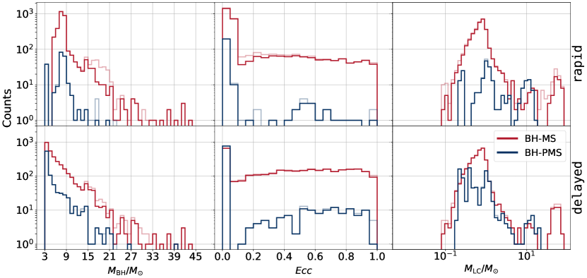
Figure 1: ${{M_{\rm{BH}}}}$, $Ecc$ and ${{M_{\rm{LC}}}}$ distributions of the present-day detached BH–LC binaries in the MW from our rapid (top) and delayed (bottom) models. The bright and faded curves represent detached BH–LCs with ${{P_{\rm{orb}}}}/{{\rm{yr}}}\leq 3$ and $10$, respectively. The red and blue curves represents BH–MS and BH–PMS, respectively. The distributions from the rapid and delayed models show significant differences between ${{M_{\rm{BH}}}}/{M_{\odot}}=3$–$5$. BHs in this range come only from AIC of NSs in the rapid model, whereas, the delayed model allows BH formation both via AIC and CCSNe in this range.

Table 1: BH–LC detectable population in the Milky Way

Model	Type	Gaia						TESS
		Optimistic			Pessimistic(${{M_{\rm{BH}}}}\geq{{M_{\rm{LC}}}}$)			Optimistic			Pessimistic(${{M_{\rm{BH}}}}\geq{{M_{\rm{LC}}}}$)
		EV	RB	SL	EV	RB	SL	EV	RB	SL	EV	RB	SL
	MS	$765^{+34}_{29}$	$1,193^{+48}_{-43}$	$77^{+13}_{-11}$	$678^{+34}_{-28}$	$920^{+37}_{-36}$	$63^{+11}_{-9}$	$176^{+16}_{-16}$	$227^{+19}_{-22}$	$3^{+3}_{-2}$	$116^{+13}_{-12}$	$149^{+15}_{-16}$	$1^{+2}_{-1}$
rapid	PMS	$256^{+18}_{-20}$	$305^{+20}_{-22}$	$24^{+5}_{-6}$	$211^{+16}_{-17}$	$238^{+17}_{-18}$	$24^{+5}_{-6}$	$78^{+13}_{-9}$	$105^{+13}_{-11}$	$1^{+2}_{-1}$	$58^{+10}_{-9}$	$47^{+8}_{-9}$	$1^{+1}_{-1}$
	total	$1,024^{+38}_{-34}$	$1,501^{+46}_{-50}$	$102^{+13}_{-13}$	$889^{+35}_{-31}$	$1,159^{+38}_{-38}$	$86^{+13}_{-10}$	$253^{+22}_{-18}$	$334^{+22}_{-23}$	$4^{+3}_{-2}$	$175^{+17}_{-16}$	$196^{+14}_{-18}$	$2^{+3}_{-1}$
	MS	$544^{+29}_{-26}$	$659^{+33}_{-30}$	$58^{+8}_{-8}$	$459^{+27}_{-26}$	$538^{+33}_{-28}$	$44^{+7}_{-8}$	$117^{+14}_{-16}$	$118^{+15}_{-14}$	$0$	$75^{+13}_{-10}$	$75^{+12}_{-12}$	$0$
delayed	PMS	$163^{+14}_{-17}$	$189^{+19}_{-17}$	$18^{+7}_{-5}$	$157^{+12}_{-17}$	$181^{+16}_{-18}$	$18^{+7}_{-5}$	$67^{+10}_{-11}$	$41^{+9}_{-9}$	$0$	$62^{+10}_{-9}$	$34^{+8}_{-8}$	$0$
	total	$707^{+35}_{-33}$	$850^{+38}_{-37}$	$76^{+11}_{-11}$	$615^{+32}_{-32}$	$719^{+35}_{-36}$	$62^{+10}_{-10}$	$183^{+22}_{-17}$	$159^{+17}_{-16}$	$0$	$136^{+17}_{-13}$	$109^{+14}_{-13}$	$0$

Note. — Number of detached BH–LC binaries in the Milky Way predicted in by models for the Gaia and TESS-detectable populations from EV, RB and SL. The numbers and errors denote the median and the spread between the $10$th and $90$th percentiles across the Milky-Way realisations.

4.1 Intrinsic BH–LC population

Figure 1 shows the distributions of ${{M_{\rm{BH}}}}$, $Ecc$, and ${{M_{\rm{LC}}}}$ of the present day detached BH–LC populations for the rapid and delayed models with the relevant upper limits on ${{P_{\rm{orb}}}}$. The characteristics of the intrinsic present-day populations depend strongly on the SNe explosion mechanism and the adopted binary evolution model which encodes mass transfer physics, stellar winds, and tidal evolution. However, we do not find significant differences between these distributions corresponding to ${{P_{\rm{orb}}}}/{{\rm{yr}}}\leq 3$ and ${{P_{\rm{orb}}}}/{{\rm{yr}}}\leq 10$. The ${{M_{\rm{BH}}}}$ distribution spans the complete allowed $3-45{M_{\odot}}$ for both rapid and delayed models, however, striking difference is apparent near the so-called ‘lower mass-gap’ between $3-5{M_{\odot}}$. While, both core-collapse SNe and AIC contribute in populating the BHs with $3\leq{{M_{\rm{BH}}}}/{M_{\odot}}\leq 5$ in the delayed model, the BHs in this mass range in the rapid model are produced from AIC only (Fryer et al., 2012). As a result, the rapid (delayed) model consists $\sim 1\%$ ($\sim 55\%$) of BH–LC binaries with ${{M_{\rm{BH}}}}/{M_{\odot}}\leq 5$. Of the BH–LCs in the delayed model with ${{M_{\rm{BH}}}}$ in the lower mass-gap, $\sim 10\%$ are produced from AIC and the rest are from core-collapse SNe.

The $Ecc$ distribution of the present-day population of BH–LC binaries transforms from the initially-assumed thermal distribution through binary stellar evolution including tides, mass loss, mass transfer, and natal kicks during BH formation. The rapid and delayed SNe prescriptions, through differences in the wind mass loss, birth mass function of BHs, and the details of the explosion mechanism, produce differences in the ${{Ecc}}$ distributions of present-day BH–LC binaries. We find that about $70\%$ of BH–LCs have near-circular ($Ecc\leq 0.1$) orbits in the rapid model, in contrast to only $40\%$ of such systems in the delayed model.

We find that the BHs with post-main sequence (PMS) companions in detached orbits with ${{P_{\rm{orb}}}}\leq 3{{\rm{yr}}}$ shows a spread of $0.1\leq{{M_{\rm{LC}}}}/{M_{\odot}}\leq 20$. BH–PMS with $20\leq{{M_{\rm{LC}}}}\leq 35{M_{\odot}}$ have ${{P_{\rm{orb}}}}\geq 10{{\rm{yr}}}$. BH–MS binaries with ${{M_{\rm{LC}}}}\leq 0.1{M_{\odot}}$ are typically found in semi-detached state. There appears to be a dearth of systems with MS companions with $18\leq{{M_{\rm{LC}}}}/{M_{\odot}}\leq 34$. This is because a relatively larger fraction of binaries have ${{P_{\rm{orb}}}}/{{\rm{yr}}}\geq 10$ in this range. About $2.1\%$ ($1.4\%$) of the present-day BH–LC population contains MS companions with ${{M_{\rm{LC}}}}/{M_{\odot}}\geq 35$ in the rapid  (delayed) model. These are young binaries with ages $\leq 10\,{{\rm Myr}}$, had initially short-period (${{P_{\rm{orb}}}}/{{\rm{yr}}}\leq 5$) orbits, which led to mass accretion via Roche-lobe overflow (RLOF) by the LC’s progenitor from the BH’s progenitor (Tout et al., 1997).

4.2 Gaia and TESS Detections

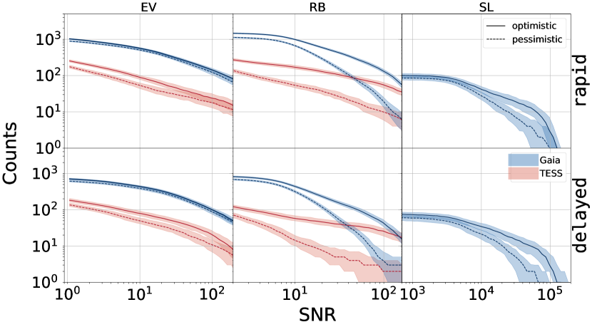
Figure 2: The reverse cumulative distribution of the expected detections of BH–LC binaries by EV (left), RB (middle) and SL (right) using TESS (red) and Gaia (blue) as a function of SNR for the rapid (top) and delayed (bottom) models. Solid and dashed lines represent the median number of detectable BH–LC binaries adopting the optimistic and pessimistic cuts (subsection 3.2). The shaded regions represent the spread between the $10$th and the $90$th percentiles due to statistical fluctuations between our 200 independent MW realisations.

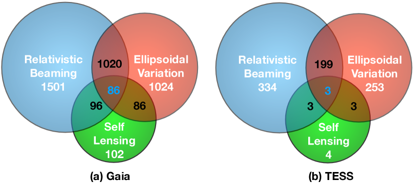
Figure 3: Number of BH–LC binaries resolvable via photometric variability by TESS (right) and Gaia (left) for the rapid model. Blue, red, and green denote populations resolvable via RB, EV, and SL signals, respectively. Numbers written in white, black, and blue denote total numbers for each set, number of systems with two and all three resolvable signals, respectively. For both telescopes, there are large ($\sim 50\%$) overlaps between populations resolvable via EV and RB. The relatively small fraction of BH–LCs with detectable SL would also be detectable either via RB or EV or both. (The equivalent figure for our delayed model is presented in the Appendix.)

Table 1 summarises the expected number of detections by Gaia and TESS via EV, RB, and SL with SNR$\geq 1$. In addition, we list the expected numbers where ${{M_{\rm{BH}}}}\geq{{M_{\rm{LC}}}}$. For both Gaia and TESS, photometric variations from EV and RB are significantly easier to detect compared to SL which leads to roughly an order of magnitude fewer detectable sources. This is expected for several reasons. In general, the geometric probability for SL is low, especially because here we consider only detached binaries which requires higher ${{P_{\rm{orb}}}}$. Even when the orientation allows SL, the magnification is typically low. Even if the maximum SL signal $\mu_{\rm{SL,max}}=[1+4/(R_{\rm{LC}}/R_{\rm{E}})^{2}]^{1/2}$ is greater than the photometric precision, the large impact parameter ($300-600R_{\rm E}$) and short transit duration ($\sim 1$ hr) makes detection challenging with the cadence we have considered for Gaia and TESS. The overall low yield from SL is consistent with past studies (Rahvar et al., 2010; Masuda & Hotokezaka, 2019; Wiktorowicz et al., 2021).

Of course, SNR$\geq 1$ may not be enough for an actual discovery. Hence, we study the expected number of detections as a function of the SNR. Figure 2 shows the reverse cumulative distribution of detached BH–LC binaries detectable via the various channels of photometric variations. For rapid, in case of Gaia, the total number of detections using the optimistic cut with SNR$\geq 1$ ($\geq 10$) is $1502$ ($1074$). The corresponding number using the pessimistic cut is $1162$ ($751$). Similarly, for TESS, the expected numbers of detections with SNR$\geq 1$ and $10$ for the optimistic (pessimistic) cut are $387$ and $194$ ($250$ and $80$).

Contribution from EV and RB are typically close to each other for both Gaia and TESS. Detected systems with EV and RB also have a high overlap (Figure 3); detectable detached BH–LC binaries with EV and RB have an overlap of roughly $50\%$ ($67\%$) for TESS (Gaia). In both Gaia and TESS, almost all detectable systems via SL can also be detected via either RB or EV or both. Overall, the expected number of detections in the rapid model is higher by a factor of $\approx 2$ compared to the delayed model. This is simply because the rapid model contains a higher proportion of higher-mass BHs compared to the delayed model (e.g., Fryer et al., 2012).

Note that, in our models, we adopt a very conservative lowest mass (${{M_{\rm{BH}}}}/{M_{\odot}}>3$) for BHs. Thus, these simulated numbers are for expected detectable BH–LC binaries with at least ${{M_{\rm{BH}}}}/{M_{\odot}}>3$. This should reduce the possibility that the unseen object is a white dwarf or NS (Fonseca et al., 2021; Romani et al., 2022). Moreover, our additional condition used in the pessimistic cut, ${{M_{\rm{BH}}}}/{{M_{\rm{LC}}}}\geq 1$, should reduce false positives even further. Nevertheless, the confidence in identifying the nature of the dark component ultimately would depend on the estimated errors in the mass and followup observations (e.g., Ganguly et al., 2023; Chakrabarti et al., 2023; El-Badry et al., 2022e; Shahaf et al., 2023). We envisage that while photometric variability can identify the interesting targets, multi-wavelength followup observations and RV followup will help to clearly identify the nature of the dark component in these binaries.

Interestingly, similar to the case of astrometrically detectable BH–LC binaries presented in Paper I, we find that the photometrically detectable BH–LC binaries also show little dependence on the BH mass (Figure 4). This can be somewhat counter-intuitive since the strength of the signal increases with increasing ${{M_{\rm{BH}}}}$ for all physical effects we have considered here (see section 3). This is because, the detectability more strongly depends on the photometric precision of Gaia and TESS compared to the signal strength. The photometric precision, on the other hand, depends strongly on the magnitude of the LC (Rimoldini, Lorenzo et al., 2023) and does not depend at all on ${{M_{\rm{BH}}}}$. As a result, the ${{M_{\rm{BH}}}}$ distribution of the detectable population is expected to closely resemble the intrinsic one. This is in contrast to BH populations detected from other more traditional observations like X-ray, radio, and GWs (Jonker et al., 2021; Liotine et al., 2023).

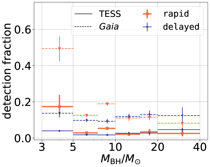
Figure 4: The ratio between the detectable binaries and intrinsic population (detection fraction) as a function of ${{M_{\rm{BH}}}}$ for the BH–LCs detectable via photometric variations using TESS (solid) and Gaia (dashed) for the rapid (orange) and delayed (blue) models. The vertical and horizontal error bars represent the $10$–$90$th percentiles and the bin size in ${{M_{\rm{BH}}}}$, respectively. The detection fraction is not strongly dependent on ${{M_{\rm{BH}}}}$ for photometrically detectable BH–LC populations from both SNe models.

4.3 Key properties of the BH–LCs detectable via photometric variations

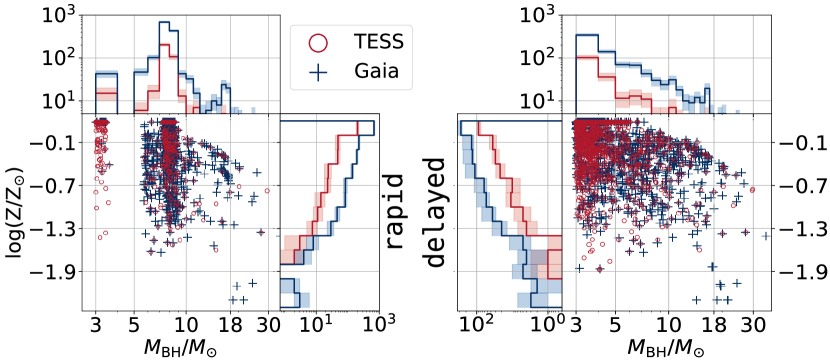
Figure 5: Distributions of ${{M_{\rm{BH}}}}$ and progenitor metallicity of the detached BH–LC binaries detectable through photometric variability. Red circle and blue plus represent populations detectable using TESS and Gaia, respectively. Lines and shades in the histograms represent median and the spread between the 10th and 90th percentiles in each bin. Left and right figures denote the rapid and delayed models.

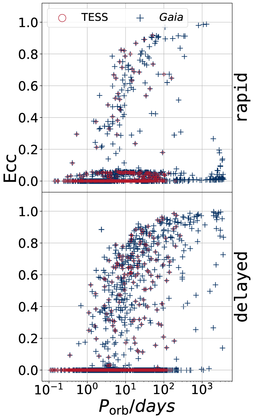
Figure 6: ${{P_{\rm{orb}}}}$ vs ${{Ecc}}$ for BH–LCs detectable via photometric variations using TESS (red circle) and Gaia (blue plus) for our rapid (top) and delayed (bottom) models.

Overall, the distributions of key observable properties for the detectable population are very similar to those of the intrinsic population. Moreover, the TESS and Gaia-detectable populations are very similar in properties. Detectable differences in the population properties come from the differences in the adopted supernova prescription.

The distributions of the detected population through photometric variability show a wide spread in both Z and ${{M_{\rm{BH}}}}$ for both the rapid and delayed models (Figure 5). The ${{M_{\rm{BH}}}}$ distribution shows distinct features for the rapid and delayed models. The lower mass gap ($3$–$5\,{M_{\odot}}$) in the intrinsic population for the rapid model remains apparent also in the detectable population; $\sim 4\%$ ($\sim 3\%$) of the TESS (Gaia) detectable BH–LC binaries contain BHs with $3\leq{{M_{\rm{BH}}}}/{M_{\odot}}\leq 5$ in the rapid model, in contrast to $\sim 65\%$ ($\sim 56\%$) in the delayed model. Of course, in the rapid model all detectable BHs in the mass gap must come from AIC of NSs. In contrast, in the delayed model, most ($\sim 85-92\%$) detectable BHs in this mass range come from core-collapse SNe while the rest come from AIC. Contribution from AIC is a little higher ($14\%$ and $8\%$ for TESS and Gaia) in the delayed model for detectable BHs with PMS companions.

The metallicities of the detectable detached BH–LCs show a wide spread, $-2.4\leq\log({{\rm Z}}/{{\rm Z}}\odot)\leq 0.2$. A majority of the detectable population consist of young BH–LC’s with ${{\rm Z}}\geq 0.02$. As a result, ${{M_{\rm{BH}}}}/{M_{\odot}}\leq 20$ in the detectable population. The wide spread in metallicities is particularly interesting. Using astrometric and photometric observations it may be possible to put constraints on the LC properties including metallicity and age. Based on these constraints, it may be possible to constrain the age and metallicity of the BH’s progenitor in real systems. Furthermore, if the mass of the BHs can also be determined via photometric variations, astrometric solutions, or follow-up observations, then a metallicity-dependent map connecting BHs with their progenitors may be found.

Apart from the ${{M_{\rm{BH}}}}$ distribution, the orbital eccentricities can also differentiate between different SN explosion mechanisms (also see Paper I). Majority ($\sim 60-98\%$) of the photometrically detectable BH–LCs in all our models go through at least one mass transfer or common-envelope episode, which erases the initial orbital eccentricity. Thus, the final orbital eccentricity is almost entirely dependent on the natal kicks the BHs receive, which later can be further modified by tides depending on ${{P_{\rm{orb}}}}$ and the time since BH formation. Under the fallback-modulated prescription for natal kicks, the BHs in the delayed model typically receive larger kicks compared to those in the rapid model. As a result, the detectable BH–LC binaries in the delayed model contain a much larger fraction ($49-56\%$) of ${{Ecc}}>0.1$ orbits compared to those in the rapid model ($8-14\%$). Figure 6 shows ${{P_{\rm{orb}}}}$ vs ${{Ecc}}$ for the detectable populations. The rapid (delayed) model contains about $92\%$ ($50\%$) and $86\%$ ($44\%$) BH–LC binaries with $Ecc\leq 0.1$ in the TESS and Gaia detected populations. Because of the relatively stronger natal kicks the BHs receive, the delayed model contains a much higher fraction ($\sim 30-40\%$) of BH–LC binaries with ${{Ecc}}>0.5$ compared to the rapid model ($5-9\%$) in the TESS as well as Gaia detected populations. These observable differences in the ${{Ecc}}$ distributions can be really interesting if detached BH–LCs are indeed discovered in large numbers through photometric as well as astrometric channels. Since, the final orbital ${{Ecc}}$ is essentially dependent on natal kicks, a careful study of the ${{Ecc}}$ distribution for these systems should help in constraining poorly understood natal kick physics (Repetto et al., 2017; Atri et al., 2019; Andrews & Kalogera, 2022; Shikauchi et al., 2023).

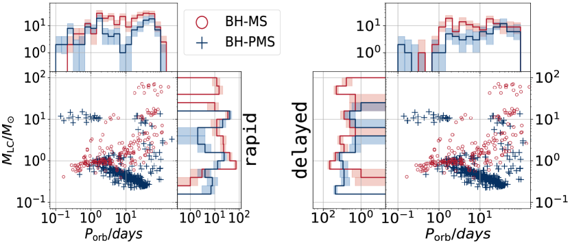
Figure 7: Distribution of ${{P_{\rm{orb}}}}$ vs ${{M_{\rm{LC}}}}$ for detached BH–LCs detectable via photometric variability using TESS. Red circles and blue crosses represent BH–MS and BH–PMS binaries, respectively. Note the correlation between ${{P_{\rm{orb}}}}$ and ${{M_{\rm{LC}}}}$, especially for the detectable BH–MS binaries.

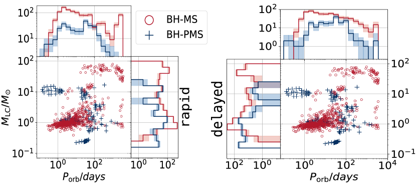
Figure 8: Same as Figure 7 but for BH–LCs detectable through photometric variability using Gaia.

We find that the ${{P_{\rm{orb}}}}$ distributions for the detectable BH–LCs exhibit diverse ranges extending up to $\sim 100$ days for TESS and $\sim 10$ years for Gaia, essentially limited by the observation duration (Figure 7, 8). At first glance this is counter-intuitive because the signal is expected to be stronger for shorter ${{P_{\rm{orb}}}}$ for all channels of photometric variability (subsubsection 3.1.1, 3.1.2). This can be understood as a consequence of subtle effects from the formation channel of the BH–LC binaries detectable through photometric variations. Most ($\approx 60-86\%$ for TESS and $84-88\%$ for Gaia) detectable BH–LCs have gone through at least one CE episode during their evolution. The eventual detached configuration, for the majority of the detectable BH–LCs thus depends on when the CE ends. All else kept fixed, a lower-mass LC would require a larger orbital decay before the CE can be ejected. This introduces a correlation between ${{P_{\rm{orb}}}}$ and ${{M_{\rm{LC}}}}$ (Figure 7, 8). A higher ${{M_{\rm{LC}}}}$ means a brighter target, which in turn means lower photometric noise, all else kept fixed. Thus, a combination of population properties as well as selection biases effectively reduces the strong ${{P_{\rm{orb}}}}$ dependence of the signal strength in the detectable population.

Overall, we find that CE evolution plays a major role in shaping the properties of the BH–LCs detectable through photometric variability. For BH–MS binaries in the rapid and delayed models, $89\%$ and $79\%$ ($80\%$ and $85\%$) of the TESS (Gaia) detectable populations go through at least one CE evolution. In case of BH–PMS binaries, between $10$ to $15\%$ of the detectable systems go through CE evolution more than once. The detectable BH–PMS binaries also show interesting clustering in the ${{P_{\rm{orb}}}}$ vs ${{M_{\rm{LC}}}}$ plane. The short-${{P_{\rm{orb}}}}$ group contains systems with significantly higher ${{M_{\rm{LC}}}}$ compared to that with longer ${{P_{\rm{orb}}}}$. The more compact BH–PMS binaries initially had massive progenitors (${{M_{\rm{LC}}}}_{\rm{ZAMS}}\geq 20\,{M_{\odot}}$) in tight orbits (${{P_{\rm{orb}}}}\lesssim 10^{2}$ days). For these binaries, the CE is initiated by mass transfer from the LC and at the time of observation, the LC is a stripped Helium star. These are all younger than $8\,{{\rm Myr}}$ at the time of observation. Because of the prevalence of CE evolution in the detectable BH–LCs, the properties of the observed populations may be able to put meaningful constraints on the uncertain aspects of CE evolution (Ivanova et al., 2013; Hirai & Mandel, 2022; Renzo et al., 2023).

5 Combination of different detection channels

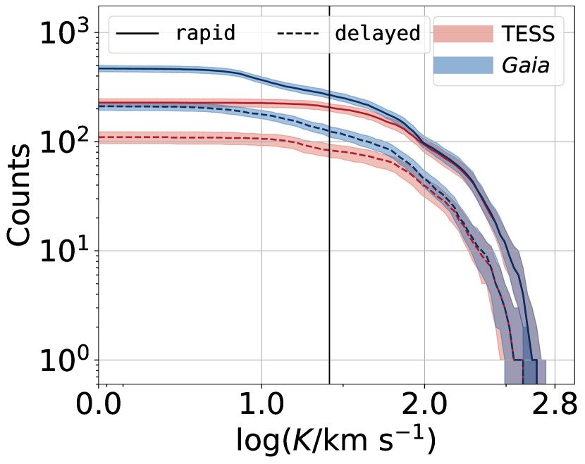
Figure 9: The reverse cumulative distribution of the RV semi-amplitude for detached BH–LCs resolvable via photometric variability using Gaia (blue) and TESS (red). The solid and dashed lines denote the rapid and delayed models. Lines denote the median and the shaded regions denote the 10th and 90th percentiles from statistical fluctuations. Black vertical line denotes the minimum resolvable $K$ by Gaia for $G\leq 17$.

Discovery of a population of stellar BHs in detached orbits with a LC is almost certainly going to receive a huge boost by combining various methods and followup studies. Indeed, several studies have identified candidate BH–LC binaries via various methods and combinations of them using Gaia’s third data release (DR3; Andrews et al., 2022; Fu et al., 2022; Gomel, R. et al., 2023; Jayasinghe et al., 2023; Shahaf et al., 2022; El-Badry et al., 2022e). In Paper I, we highlighted that a large population of detached BH–LC binaries may be resolvable by Gaia’s astrometry and that astrometry alone is likely to put strong enough constraints on the dark object’s mass to clearly indicate a BH. Furthermore, we highlighted that Gaia’s RV with a spectral resolution of $R\sim 11,500$ for stars brighter than $G=17$ (Cropper, M. et al., 2018; Soubiran, C. et al., 2018; Sartoretti, P. et al., 2023), itself could resolve the orbital motion for $\sim 50-120$ astrometrically resolvable binaries depending on the model assumptions. Of course, once the candidates are identified, spectroscopic followup using higher-precision instruments can significantly improve these yields, but since Gaia’s RV will automatically become available without any need for extensive followup, we only focus on that.

Figure 9 shows the reverse cumulative distribution of the RV semi-amplitude for BH–LCs brighter than $G=17$ and resolvable through photometric variability by TESS and Gaia. The vertical line shows Gaia’s spectral resolution cutoff for $G\leq 17$. We find that $207^{+19}_{-18}$ ($268^{+25}_{-19}$) and $83^{+12}_{-11}$( $124^{+13}_{-12}$ ) BH–LCs in the TESS (Gaia) resolved population would also be resolved with the help of spectroscopy in the rapid and delayed models, respectively. Interestingly, $25\%$–$60\%$ of all photometrically detectable BH–LC binaries brighter than $G=17$, ($15$–$30\%$ overall) are expected to have RV resolvable by Gaia. Thus, a combination of photometric detection and Gaia’s RV analysis is expected to provide credence to these discoveries and allow better characterisation of orbital and stellar properties.

Figure 10 shows the detection fraction as function of ${{P_{\rm{orb}}}}$ for detached BH–LCs detected via TESS and Gaia photometry and Gaia’s astrometry. In case of Gaia’s astrometry, the detection fraction monotonically increases until it saturates for ${{P_{\rm{orb}}}}\gtrsim 100$ days. This of course is easy to understand; the larger the orbit, the easier it is to resolve via astrometry. The trend for the photometrically resolvable populations is more nuanced. In this case, both for Gaia and TESS, the detection fraction first increases with increasing ${{P_{\rm{orb}}}}$, peaks around ${{P_{\rm{orb}}}}/{\rm{day}}=10$–$100$ (${{P_{\rm{orb}}}}/{\rm{day}}=100$–$1,000$) for TESS (Gaia) before decreasing. The peak is created due to the competition between two separate effects. The photometric variability signal depends strongly on ${{P_{\rm{orb}}}}$, the more compact the orbit, the stronger the signal. As a result, for sufficiently large ${{P_{\rm{orb}}}}$, the signal is simply too weak resulting in a decrease in the detection fraction. On the other hand, most detectable BH–LCs come from CE evolution. As a result, there is a distinct correlation between ${{P_{\rm{orb}}}}$ and ${{M_{\rm{LC}}}}$ (Figure 7, 8) and as a result, the magnitude. Hence, as ${{P_{\rm{orb}}}}$ increases, the photometric variability is easier to detect because of the lower noise for the brighter LCs. The different locations of the peaks for Gaia and TESS are reflective of their different observation duration.

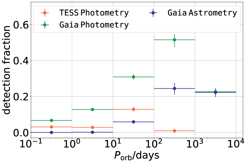
Figure 10: Detection fraction of detached BH–LC binaries as a function of ${{P_{\rm{orb}}}}$ via Gaia’s astrometry (blue), TESS photometry (orange), and Gaia’s photometry (green) for the rapid model. Dots and error bars represent median, 10th, and 90th percentiles in each bin. Detection fraction via astrometry increases with increasing ${{P_{\rm{orb}}}}$ until it saturates for ${{P_{\rm{orb}}}}/{\rm{day}}\gtrsim 10^{2}$. In contrast, detection fraction from photometry exhibits a peak. At large ${{P_{\rm{orb}}}}$, the decrease from the peak detection fraction is due to reduced photometric variability signal, whereas, at the small ${{P_{\rm{orb}}}}$, the decrease is due to the correlation between ${{P_{\rm{orb}}}}$ and ${{M_{\rm{LC}}}}$ in the BH-LC binaries (Figure 7,8). (The equivalent figure for our delayed model is presented in the Appendix.)

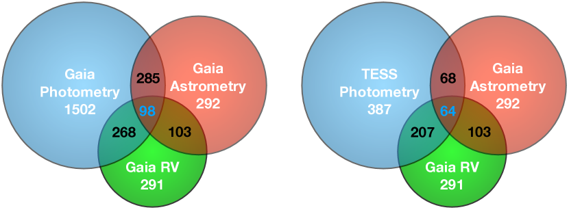
Figure 11: The expected numbers of detections from photomety (blue), Gaia’s astrometry (red), and Gaia’s RV (green) for detached BH–LC population for the rapid model and their overlap. The white, black, and blue numbers denote yields in each set, overlap between two, and three different channels, respectively. (The equivalent figure for our delayed model is presented in the Appendix.)

Figure 11 shows the expected yields for detached BH–LCs from different detection channels and the overlap. We find between $11-19\%$ (depending on the adopted SNe model) of the photometrically detectable BH–LCs would also be resolvable via astrometry. On the other hand, between $14-50\%$ of the photometrically detectable BH–LCs are expected to have sufficiently large RV that this can be resolved by Gaia’s RV. Overall, about $5-16\%$ of all BH–LCs could be detectable from astrometry, photometry, as well as RV.

6 Summary and Discussions

We have explored the possibility of detecting detached BH–LC binaries via photometric variability with TESS and Gaia. We create highly realistic present-day BH–LC populations using the BPS suite COSMIC (Breivik et al., 2020) taking into account a metallicity-dependent star formation history and the complex correlations between age, metallicity, and location of stars in the Milky Way (Wetzel et al., 2016; Hopkins et al., 2018; Sanderson et al., 2020). We have used two widely adopted SNe explosion mechanisms, rapid and delayed (Fryer et al., 2012), to create two separate populations of present-day BH–LC binaries. We have shown the key observable features of the intrinsic BH–LC populations adopting appropriate ${{P_{\rm{orb}}}}$ limits (see subsection 4.1) as well as those that are expected to be detected via photometric variability (see subsection 4.2).

Using 200 realisations to take into account statistical fluctuations, taking into account different physical sources for photometric variability, TESS and Gaia selection biases, and three-dimensional extinction and reddening, we have generated a highly realistic population of detectable detached BH–LC binaries in the Milky Way at present (subsection 2.1, 3.2). In addition to detection through photometric variability, we have also analysed Gaia’s RV and astrometry to find relative yield and sources that could be detectable via multiple channels (see section 5).

• We predict about $100-400$ and $700-1500$ detached BH–LC binaries may detected by TESS and Gaia through photometric variability arising primarily from EV and RB.

• The photometrically detectable BH–LCs are expected to have wide range in metallicity and host BHs spanning a wide range in mass (see Figure 5). This is potentially interesting since in such systems, if the LC properties such as age and metallicity can be observationally constrained, we may be able to find a direct connection between the BHs and their progenitor properties.

• The detection fraction is not strongly dependent on the BH mass (Figure 4). Thus, the detectable BHs are expected to be similar in properties to the intrinsic BHs in detached BH–LC binaries.

• The orbital ${{Ecc}}$ is essentially determined by BH natal kicks. As a result, if detected in large numbers, the ${{Ecc}}$ distribution can put constraints on natal kicks from core-collapse SNe.

• Since a majority ($\sim 60-90\%$) of BH–LCs detectable through photometric variability using TESS and Gaia go through at least one CE episode, there is an interesting correlation between ${{P_{\rm{orb}}}}$ and ${{M_{\rm{LC}}}}$, especially for BH–MS binaries (Figure 7, 8). It will be interesting to verify this trend. Moreover, since this stems primarily from the energetics of envelope ejection, if detected in large numbers as we predict, this population may put meaningful constraints on the various uncertain aspects of CE physics.

• A significant fraction of photometrically detectable BH–LC binaries may also be detectable via Gaia’s RV and astrometry ($5$–$16\%$ are detectable via all three methods, Figure 9, Figure 11), thus helping provide stronger constraints on their properties.

In Paper I, we showed the potential of Gaia’s astrometry for detecting and characterizing detached BH–LC binaries in large numbers. In this work we show that a combination of photometry, RV, and astrometry can significantly increase the number of identified detached BH–LC candidates. Especially, many detached BH–LCs are expected to be detectable via astrometry, RV, as well as photometry. Once identified, followup observations using more sophisticated instruments may improve the characterisation of these candidates even further. Our models suggest that we are on the verge of discovering a treasure trove in BH binaries, while the recent BH discoveries from Gaia astrometry (El-Badry et al., 2022e, 2023; Chakrabarti et al., 2023) whet our enthusiasm.

Here we present selected results from our delayed model. Figure 12 shows the detection fraction as a function of ${{P_{\rm{orb}}}}$ for the delayed model for our detected population of BH-LC binaries. The detection fraction in the delayed model is very similar to the same for the rapid model (Figure 10).

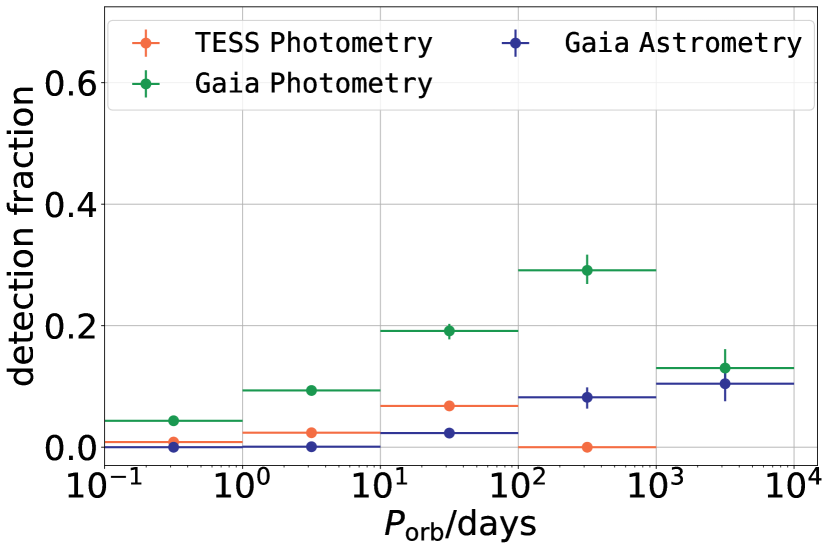
Figure 12: Same as Figure 10 but for the BH-LCs in our delayed model.

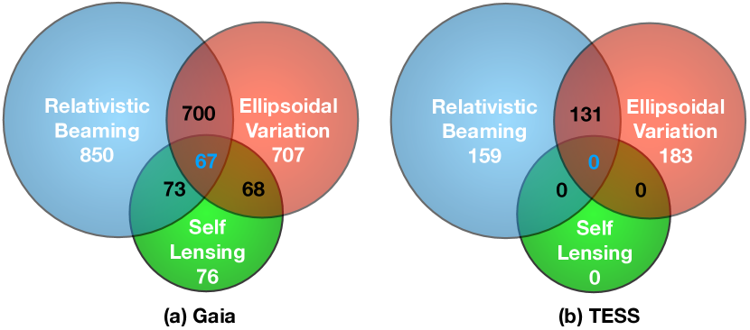
Figure 13: Same as Figure 3 but for the BH-LCs in our delayed model.

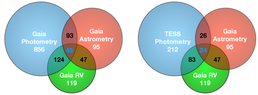
Figure 14: Same as Figure 11 but for the BH-LCs in our delayed model.

References

- Abbott et al. (2016a) Abbott, B. P., Abbott, R., Abbott, T. D., et al. 2016a, Phys. Rev. Lett., 116, 1, doi: 10.1103/PhysRevLett.116.061102
- Abbott et al. (2016b) —. 2016b, Phys. Rev. Lett., 116, 1, doi: 10.1103/PhysRevLett.116.241103
- Abbott et al. (2019) —. 2019, Phys. Rev. X, 9, 031040, doi: 10.1103/PhysRevX.9.031040
- Abbott et al. (2021a) Abbott, R., Abbott, T. D., Abraham, S., et al. 2021a, Physical Review X, 11, 021053, doi: 10.1103/PhysRevX.11.021053
- Abbott et al. (2021b) —. 2021b, ApJ, 913, L7, doi: 10.3847/2041-8213/abe949
- Abdurrahman et al. (2021) Abdurrahman, F. N., Stephens, H. F., & Lu, J. R. 2021, The Astrophysical Journal, 912, 146, doi: 10.3847/1538-4357/abee83
- Alonso et al. (2004) Alonso, R., Brown, T. M., Torres, G., et al. 2004, The Astrophysical Journal, 613, L153, doi: 10.1086/425256
- Ambartsumian (1937) Ambartsumian, V. A. 1937, AZh, 14, 207
- Andrews et al. (2019) Andrews, J. J., Breivik, K., & Chatterjee, S. 2019, The Astrophysical Journal, 886, 68, doi: 10.3847/1538-4357/ab441f
- Andrews & Kalogera (2022) Andrews, J. J., & Kalogera, V. 2022, The Astrophysical Journal, 930, 159, doi: 10.3847/1538-4357/ac66d6
- Andrews et al. (2022) Andrews, J. J., Taggart, K., & Foley, R. 2022, arXiv e-prints, arXiv:2207.00680. https://arxiv.org/abs/2207.00680
- Angus et al. (2019) Angus, R., Morton, T. D., Foreman-Mackey, D., et al. 2019, The Astronomical Journal, 158, 173, doi: 10.3847/1538-3881/ab3c53
- Astropy Collaboration et al. (2013) Astropy Collaboration, Robitaille, T. P., Tollerud, E. J., et al. 2013, A&A, 558, A33, doi: 10.1051/0004-6361/201322068
- Atri et al. (2019) Atri, P., Miller-Jones, J. C. A., Bahramian, A., et al. 2019, Monthly Notices of the Royal Astronomical Society, 489, 3116, doi: 10.1093/mnras/stz2335
- Auvergne, M. et al. (2009) Auvergne, M., Bodin, P., Boisnard, L., et al. 2009, A&A, 506, 411, doi: 10.1051/0004-6361/200810860
- Bakos et al. (2004) Bakos, G., Noyes, R. W., Kovács, G., et al. 2004, Publications of the Astronomical Society of the Pacific, 116, 266, doi: 10.1086/382735
- Barclay (2017) Barclay, T. 2017, tessgi/ticgen: v1.0.0, v1.0.0, Zenodo, Zenodo, doi: 10.5281/zenodo.888217
- Barstow et al. (2014) Barstow, M. A., Casewell, S. L., Catalan, S., et al. 2014, arXiv e-prints, arXiv:1407.6163. https://arxiv.org/abs/1407.6163
- Belczynski et al. (2008) Belczynski, K., Kalogera, V., Rasio, F. A., et al. 2008, Astrophys. J. Suppl. Ser., 174, 223, doi: 10.1086/521026
- Bellinger, E. P. et al. (2019) Bellinger, E. P., Hekker, S., Angelou, G. C., Stokholm, A., & Basu, S. 2019, A&A, 622, A130, doi: 10.1051/0004-6361/201834461
- Bellm et al. (2018) Bellm, E. C., Kulkarni, S. R., Graham, M. J., et al. 2018, Publications of the Astronomical Society of the Pacific, 131, 018002, doi: 10.1088/1538-3873/aaecbe
- Bloemen et al. (2011) Bloemen, S., Marsh, T. R., Østensen, R. H., et al. 2011, Monthly Notices of the Royal Astronomical Society, 410, 1787, doi: 10.1111/j.1365-2966.2010.17559.x
- Borucki et al. (2011) Borucki, W. J., Koch, D. G., Basri, G., et al. 2011, The Astrophysical Journal, 736, 19, doi: 10.1088/0004-637x/736/1/19
- Bovy et al. (2016) Bovy, J., Rix, H.-W., Green, G. M., Schlafly, E. F., & Finkbeiner, D. P. 2016, The Astrophysical Journal, 818, 130, doi: 10.3847/0004-637x/818/2/130
- Breivik et al. (2019) Breivik, K., Chatterjee, S., & Andrews, J. J. 2019, ApJ, 878, L4, doi: 10.3847/2041-8213/ab21d3
- Breivik et al. (2017) Breivik, K., Chatterjee, S., & Larson, S. L. 2017, The Astrophysical Journal, 850, L13, doi: 10.3847/2041-8213/aa97d5
- Breivik et al. (2020) Breivik, K., Coughlin, S., Zevin, M., et al. 2020, ApJ, 898, 71, doi: 10.3847/1538-4357/ab9d85
- Brown & Bethe (1994) Brown, G. E., & Bethe, H. A. 1994, Astrophys. J., 423, doi: 10.1086/173844
- Brown (2003) Brown, T. M. 2003, The Astrophysical Journal, 593, L125, doi: 10.1086/378310
- Burke et al. (2020) Burke, C. J., Levine, A., Fausnaugh, M., et al. 2020, TESS-Point: High precision TESS pointing tool, Astrophysics Source Code Library. http://ascl.net/2003.001
- Casares et al. (2014) Casares, J., Negueruela, I., Ribó, M., et al. 2014, Nature, 505, 378, doi: 10.1038/nature12916
- Chakrabarti et al. (2023) Chakrabarti, S., Simon, J. D., Craig, P. A., et al. 2023, The Astronomical Journal, 166, 6, doi: 10.3847/1538-3881/accf21
- Chawla et al. (2022) Chawla, C., Chatterjee, S., Breivik, K., et al. 2022, The Astrophysical Journal, 931, 107, doi: 10.3847/1538-4357/ac60a5
- Claeys et al. (2014) Claeys, J. S. W., Pols, O. R., Izzard, R. G., Vink, J., & Verbunt, F. W. M. 2014, A&A, 563, A83, doi: 10.1051/0004-6361/201322714
- Cropper, M. et al. (2018) Cropper, M., Katz, D., Sartoretti, P., et al. 2018, A&A, 616, A5, doi: 10.1051/0004-6361/201832763
- Drimmel et al. (2003) Drimmel, R., Cabrera-Lavers, A., & López-Corredoira, M. 2003, Astron. Astrophys., 409, 205, doi: 10.1051/0004-6361:20031070
- Duchêne & Kraus (2013) Duchêne, G., & Kraus, A. 2013, Annual Review of Astronomy and Astrophysics, 51, 269, doi: 10.1146/annurev-astro-081710-102602
- El-Badry & Burdge (2022) El-Badry, K., & Burdge, K. B. 2022, Monthly Notices of the Royal Astronomical Society: Letters, 511, 24, doi: 10.1093/mnrasl/slab135
- El-Badry et al. (2022a) El-Badry, K., Burdge, K. B., & Mróz, P. 2022a, Monthly Notices of the Royal Astronomical Society, 511, 3089, doi: 10.1093/mnras/stac274
- El-Badry & Quataert (2021) El-Badry, K., & Quataert, E. 2021, Monthly Notices of the Royal Astronomical Society, 502, 3436, doi: 10.1093/mnras/stab285
- El-Badry et al. (2022b) El-Badry, K., Seeburger, R., Jayasinghe, T., et al. 2022b, Monthly Notices of the Royal Astronomical Society, 512, 5620, doi: 10.1093/mnras/stac815
- El-Badry et al. (2022e) El-Badry, K., Rix, H.-W., Quataert, E., et al. 2022e, Monthly Notices of the Royal Astronomical Society, 518, 1057, doi: 10.1093/mnras/stac3140
- El-Badry et al. (2023) El-Badry, K., Rix, H.-W., Cendes, Y., et al. 2023, Monthly Notices of the Royal Astronomical Society, 521, 4323, doi: 10.1093/mnras/stad799
- Engel et al. (2020) Engel, M., Faigler, S., Shahaf, S., & Mazeh, T. 2020, Monthly Notices of the Royal Astronomical Society, 497, 4884, doi: 10.1093/mnras/staa2182
- Fonseca et al. (2021) Fonseca, E., Cromartie, H. T., Pennucci, T. T., et al. 2021, The Astrophysical Journal Letters, 915, L12, doi: 10.3847/2041-8213/ac03b8
- Fryer et al. (2012) Fryer, C. L., Belczynski, K., Wiktorowicz, G., et al. 2012, Astrophys. J., 749, doi: 10.1088/0004-637X/749/1/91
- Fryer et al. (2022) Fryer, C. L., Olejak, A., & Belczynski, K. 2022, ApJ, 931, 94, doi: 10.3847/1538-4357/ac6ac9
- Fu et al. (2022) Fu, J.-B., Gu, W.-M., Zhang, Z.-X., et al. 2022, The Astrophysical Journal, 940, 126, doi: 10.3847/1538-4357/ac9b4c
- Fuchs & Bastian (2005) Fuchs, B., & Bastian, U. 2005, in ESA Special Publication, Vol. 576, The Three-Dimensional Universe with Gaia, ed. C. Turon, K. S. O’Flaherty, & M. A. C. Perryman, 573
- Gaia Collaboration et al. (2023) Gaia Collaboration, Arenou, F., Babusiaux, C., et al. 2023, A&A, 674, A34, doi: 10.1051/0004-6361/202243782
- Ganguly et al. (2023) Ganguly, A., Nayak, P. K., & Chatterjee, S. 2023, The Astrophysical Journal, 954, 4, doi: 10.3847/1538-4357/ace42f
- Giesers et al. (2018) Giesers, B., Dreizler, S., Husser, T. O., et al. 2018, Mon. Not. R. Astron. Soc. Lett., 475, L15, doi: 10.1093/mnrasl/slx203
- Giesers et al. (2019) Giesers, B., Kamann, S., Dreizler, S., et al. 2019, A&A, 632, A3, doi: 10.1051/0004-6361/201936203
- Goldberg & Mazeh (1994) Goldberg, D., & Mazeh, T. 1994, A&A, 282, 801
- Gomel et al. (2020) Gomel, R., Faigler, S., & Mazeh, T. 2020, Monthly Notices of the Royal Astronomical Society, 501, 2822, doi: 10.1093/mnras/staa3305
- Gomel, R. et al. (2023) Gomel, R., Mazeh, T., Faigler, S., et al. 2023, A&A, 674, A19, doi: 10.1051/0004-6361/202243626
- Gomez & Grindlay (2021) Gomez, S., & Grindlay, J. E. 2021, The Astrophysical Journal, 913, 48, doi: 10.3847/1538-4357/abf24c
- Gould (1995) Gould, A. 1995, ApJ, 446, 541, doi: 10.1086/175812
- Gould & Salim (2002) Gould, A., & Salim, S. 2002, ApJ, 572, 944, doi: 10.1086/340435
- Green et al. (2019) Green, G. M., Schlafly, E., Zucker, C., Speagle, J. S., & Finkbeiner, D. 2019, The Astrophysical Journal, 887, 93, doi: 10.3847/1538-4357/ab5362
- Han (1998) Han, Z. 1998, MNRAS, 296, 1019, doi: 10.1046/j.1365-8711.1998.01475.x
- Heggie (1975) Heggie, D. C. 1975, Mon. Not. R. Astron. Soc., 173, doi: 10.1093/mnras/173.3.729
- Herrero, E. et al. (2014) Herrero, E., Lanza, A. F., Ribas, I., et al. 2014, A&A, 563, A104, doi: 10.1051/0004-6361/201323087
- Hirai & Mandel (2022) Hirai, R., & Mandel, I. 2022, The Astrophysical Journal Letters, 937, L42, doi: 10.3847/2041-8213/ac9519
- Hobbs et al. (2005) Hobbs, G., Lorimer, D. R., Lyne, A. G., & Kramer, M. 2005, Mon. Not. R. Astron. Soc., 360, doi: 10.1111/j.1365-2966.2005.09087.x
- Hopkins et al. (2018) Hopkins, P. F., Wetzel, A., Kereš, D., et al. 2018, MNRAS, 480, 800, doi: 10.1093/mnras/sty1690
- Hu et al. (2023) Hu, Z.-C., Yang, Y.-L., Wen, Y.-H., Shen, R.-F., & Tam, P.-H. T. 2023, Research in Astronomy and Astrophysics, 23, 085008, doi: 10.1088/1674-4527/accc73
- Hunter (2007) Hunter, J. D. 2007, Computing in Science and Engineering, 9, 90, doi: 10.1109/MCSE.2007.55
- Hurley et al. (2000) Hurley, J. R., Pols, O. R., & Tout, C. A. 2000, MNRAS, 315, 543, doi: 10.1046/j.1365-8711.2000.03426.x
- Hurley et al. (2002) Hurley, J. R., Tout, C. A., & Pols, O. R. 2002, Mon. Not. R. Astron. Soc., 329, doi: 10.1046/j.1365-8711.2002.05038.x
- Ivanova et al. (2013) Ivanova, N., Justham, S., Chen, X., et al. 2013, A&A Rev., 21, 59, doi: 10.1007/s00159-013-0059-2
- Ivezić et al. (2019) Ivezić, Ž., Kahn, S. M., Tyson, J. A., et al. 2019, ApJ, 873, 111, doi: 10.3847/1538-4357/ab042c
- Janssens et al. (2022) Janssens, S., Shenar, T., Sana, H., et al. 2022, A&A, 658, A129, doi: 10.1051/0004-6361/202141866
- Jayasinghe et al. (2023) Jayasinghe, T., Rowan, D. M., Thompson, T. A., Kochanek, C. S., & Stanek, K. Z. 2023, Monthly Notices of the Royal Astronomical Society, 521, 5927, doi: 10.1093/mnras/stad909
- Jayasinghe et al. (2021) Jayasinghe, T., Stanek, K. Z., Thompson, T. A., et al. 2021, MNRAS, 504, 2577, doi: 10.1093/mnras/stab907
- Jeans (1919) Jeans, J. H. 1919, Monthly Notices of the Royal Astronomical Society, 79, 408, doi: 10.1093/mnras/79.6.408
- Jonker et al. (2021) Jonker, P. G., Kaur, K., Stone, N., & Torres, M. A. P. 2021, The Astrophysical Journal, 921, 131, doi: 10.3847/1538-4357/ac2839
- Kane et al. (2016) Kane, S. R., Thirumalachari, B., Henry, G. W., et al. 2016, The Astrophysical Journal, 820, L5, doi: 10.3847/2041-8205/820/1/l5
- Khokhlov et al. (2018) Khokhlov, S. A., Miroshnichenko, A. S., Zharikov, S. V., et al. 2018, The Astrophysical Journal, 856, 158, doi: 10.3847/1538-4357/aab49d
- Khruzina et al. (1988) Khruzina, T., Cherepaschuk, A., Shakura, N., & Sunyaev, R. 1988, Advances in Space Research, 8, 237, doi: https://doi.org/10.1016/0273-1177(88)90413-9
- Kochanek et al. (2017) Kochanek, C. S., Shappee, B. J., Stanek, K. Z., et al. 2017, Publications of the Astronomical Society of the Pacific, 129, 104502, doi: 10.1088/1538-3873/aa80d9
- Kollmeier et al. (2017) Kollmeier, J. A., Zasowski, G., Rix, H.-W., et al. 2017, arXiv e-prints, arXiv:1711.03234, doi: 10.48550/arXiv.1711.03234
- Kopal (1959) Kopal, Z. 1959, Close binary systems
- Kroupa (2001) Kroupa, P. 2001, Mon. Not. R. Astron. Soc., 322, doi: 10.1046/j.1365-8711.2001.04022.x
- Lam et al. (2022) Lam, C. Y., Lu, J. R., Udalski, A., et al. 2022, The Astrophysical Journal Letters, 933, L23, doi: 10.3847/2041-8213/ac7442
- Leibovitz & Hube (1971) Leibovitz, C., & Hube, D. P. 1971, A&A, 15, 251
- Lennon, D. J. et al. (2022) Lennon, D. J., Dufton, P. L., Villaseñor, J. I., et al. 2022, A&A, 665, A180, doi: 10.1051/0004-6361/202142413
- Lin et al. (2018) Lin, J., Dotter, A., Ting, Y.-S., & Asplund, M. 2018, Monthly Notices of the Royal Astronomical Society, 477, 2966, doi: 10.1093/mnras/sty709
- Liotine et al. (2023) Liotine, C., Zevin, M., Berry, C. P. L., Doctor, Z., & Kalogera, V. 2023, The Astrophysical Journal, 946, 4, doi: 10.3847/1538-4357/acb8b2
- Liu et al. (2019) Liu, J., Zhang, H., Howard, A. W., et al. 2019, Nature, 575, 618, doi: 10.1038/s41586-019-1766-2
- Livio & Soker (1984) Livio, M., & Soker, N. 1984, Monthly Notices of the Royal Astronomical Society, 208, 763, doi: 10.1093/mnras/208.4.763
- Loeb & Gaudi (2003) Loeb, A., & Gaudi, B. S. 2003, The Astrophysical Journal, 588, L117, doi: 10.1086/375551
- Maeder (1973) Maeder, A. 1973, A&A, 26, 215
- Marshall et al. (2006) Marshall, D. J., Robin, A. C., Reylé, C., Schultheis, M., & Picaud, S. 2006, Astron. Astrophys., 453, 635, doi: 10.1051/0004-6361:20053842
- Mashian & Loeb (2017) Mashian, N., & Loeb, A. 2017, Mon. Not. R. Astron. Soc., 470, doi: 10.1093/mnras/stx1410
- Masuda & Hotokezaka (2019) Masuda, K., & Hotokezaka, K. 2019, Astrophys. J., 883, 169, doi: 10.3847/1538-4357/ab3a4f
- Mazeh et al. (1992) Mazeh, T., Goldberg, D., Duquennoy, A., & Mayor, M. 1992, ApJ, 401, 265, doi: 10.1086/172058
- McCullough et al. (2005) McCullough, P. R., Stys, J. E., Valenti, J. A., et al. 2005, Publications of the Astronomical Society of the Pacific, 117, 783, doi: 10.1086/432024
- Meurer et al. (2017) Meurer, A., Smith, C. P., Paprocki, M., et al. 2017, PeerJ Computer Science, 3, e103, doi: 10.7717/peerj-cs.103
- Moe & Stefano (2017) Moe, M., & Stefano, R. D. 2017, The Astrophysical Journal Supplement Series, 230, 15, doi: 10.3847/1538-4365/aa6fb6
- Morris (1985) Morris, S. 1985, ApJ, 295, 143, doi: 10.1086/163359
- Morris & Naftilan (1993) Morris, S. L., & Naftilan, S. A. 1993, ApJ, 419, 344, doi: 10.1086/173488
- Morton (2015) Morton, T. D. 2015, isochrones: Stellar model grid package. http://ascl.net/1503.010
- Mróz et al. (2022) Mróz, P., Udalski, A., & Gould, A. 2022, The Astrophysical Journal Letters, 937, L24, doi: 10.3847/2041-8213/ac90bb
- Nagarajan et al. (2023) Nagarajan, P., El-Badry, K., Rodriguez, A. C., van Roestel, J., & Roulston, B. 2023, Monthly Notices of the Royal Astronomical Society, 524, 4367, doi: 10.1093/mnras/stad2130
- Nie et al. (2017) Nie, J. D., Wood, P. R., & Nicholls, C. P. 2017, The Astrophysical Journal, 835, 209, doi: 10.3847/1538-4357/835/2/209
- Olejak, A. et al. (2020) Olejak, A., Belczynski, K., Bulik, T., & Sobolewska, M. 2020, A&A, 638, A94, doi: 10.1051/0004-6361/201936557
- Patton & Sukhbold (2020) Patton, R. A., & Sukhbold, T. 2020, MNRAS, 499, 2803, doi: 10.1093/mnras/staa3029
- Patton et al. (2022) Patton, R. A., Sukhbold, T., & Eldridge, J. J. 2022, Monthly Notices of the Royal Astronomical Society, 511, 903, doi: 10.1093/mnras/stab3797
- Pepper et al. (2007) Pepper, J., Pogge, R. W., DePoy, D. L., et al. 2007, Publications of the Astronomical Society of the Pacific, 119, 923, doi: 10.1086/521836
- Pollacco et al. (2006) Pollacco, D. L., Skillen, I., Cameron, A. C., et al. 2006, Publications of the Astronomical Society of the Pacific, 118, 1407, doi: 10.1086/508556
- Predehl et al. (2021) Predehl, P., Andritschke, R., Arefiev, V., et al. 2021, A&A, 647, A1, doi: 10.1051/0004-6361/202039313
- Price-Whelan et al. (2018) Price-Whelan, A. M., Sipőcz, B. M., Günther, H. M., et al. 2018, AJ, 156, 123, doi: 10.3847/1538-3881/aabc4f
- Qian et al. (2008) Qian, S.-B., Liao, W.-P., & Lajús, E. F. 2008, The Astrophysical Journal, 687, 466, doi: 10.1086/591515
- Rahvar et al. (2010) Rahvar, S., Mehrabi, A., & Dominik, M. 2010, Monthly Notices of the Royal Astronomical Society, 410, 912, doi: 10.1111/j.1365-2966.2010.17490.x
- Renzo et al. (2023) Renzo, M., Zapartas, E., Justham, S., et al. 2023, The Astrophysical Journal Letters, 942, L32, doi: 10.3847/2041-8213/aca4d3
- Repetto et al. (2017) Repetto, S., Igoshev, A. P., & Nelemans, G. 2017, Monthly Notices of the Royal Astronomical Society, 467, 298, doi: 10.1093/mnras/stx027
- Ricker et al. (2014) Ricker, G. R., Winn, J. N., Vanderspek, R., et al. 2014, in Space Telescopes and Instrumentation 2014: Optical, Infrared, and Millimeter Wave, ed. J. M. O. Jr., M. Clampin, G. G. Fazio, & H. A. MacEwen, Vol. 9143, International Society for Optics and Photonics (SPIE), 556 – 570. https://doi.org/10.1117/12.2063489
- Rimoldini, Lorenzo et al. (2023) Rimoldini, Lorenzo, Holl, Berry, Gavras, Panagiotis, et al. 2023, A&A, 674, A14, doi: 10.1051/0004-6361/202245591
- Rivinius, Th. et al. (2020) Rivinius, Th., Baade, D., Hadrava, P., Heida, M., & Klement, R. 2020, A&A, 637, L3, doi: 10.1051/0004-6361/202038020
- Romani et al. (2022) Romani, R. W., Kandel, D., Filippenko, A. V., Brink, T. G., & Zheng, W. 2022, The Astrophysical Journal Letters, 934, L17, doi: 10.3847/2041-8213/ac8007
- Sahu et al. (2022) Sahu, K. C., Anderson, J., Casertano, S., et al. 2022, The Astrophysical Journal, 933, 83, doi: 10.3847/1538-4357/ac739e
- Sanderson et al. (2020) Sanderson, R. E., Wetzel, A., Loebman, S., et al. 2020, Astrophys. J. Suppl. Ser., 246, doi: 10.3847/1538-4365/ab5b9d
- Saracino et al. (2021) Saracino, S., Kamann, S., Guarcello, M. G., et al. 2021, Monthly Notices of the Royal Astronomical Society, 511, 2914, doi: 10.1093/mnras/stab3159
- Sartoretti, P. et al. (2023) Sartoretti, P., Marchal, O., Babusiaux, C., et al. 2023, A&A, 674, A6, doi: 10.1051/0004-6361/202243615
- Shahaf et al. (2022) Shahaf, S., Bashi, D., Mazeh, T., et al. 2022, Monthly Notices of the Royal Astronomical Society, 518, 2991, doi: 10.1093/mnras/stac3290
- Shahaf et al. (2023) Shahaf, S., Hallakoun, N., Mazeh, T., et al. 2023, arXiv e-prints, arXiv:2309.15143, doi: 10.48550/arXiv.2309.15143
- Shahaf et al. (2019) Shahaf, S., Mazeh, T., Faigler, S., & Holl, B. 2019, Monthly Notices of the Royal Astronomical Society, 487, 5610, doi: 10.1093/mnras/stz1636
- Shakura & Postnov (1987) Shakura, N. I., & Postnov, K. A. 1987, A&A, 183, L21
- Shappee et al. (2014) Shappee, B. J., Prieto, J. L., Grupe, D., et al. 2014, The Astrophysical Journal, 788, 48, doi: 10.1088/0004-637x/788/1/48
- Shenar et al. (2022a) Shenar, T., Sana, H., Mahy, L., et al. 2022a, Nature Astronomy, 6, 1085, doi: 10.1038/s41550-022-01730-y
- Shenar et al. (2022b) —. 2022b, A&A, 665, A148, doi: 10.1051/0004-6361/202244245
- Shikauchi et al. (2023) Shikauchi, M., Tsuna, D., Tanikawa, A., & Kawanaka, N. 2023, The Astrophysical Journal, 953, 52, doi: 10.3847/1538-4357/acd752
- Shporer (2017) Shporer, A. 2017, Publications of the Astronomical Society of the Pacific, 129, 072001, doi: 10.1088/1538-3873/aa7112
- Simpson et al. (2022) Simpson, E. R., Fetherolf, T., Kane, S. R., et al. 2022, The Astronomical Journal, 163, 215, doi: 10.3847/1538-3881/ac5d41
- Soubiran, C. et al. (2018) Soubiran, C., Jasniewicz, G., Chemin, L., et al. 2018, A&A, 616, A7, doi: 10.1051/0004-6361/201832795
- Stassun et al. (2018) Stassun, K. G., Oelkers, R. J., Pepper, J., et al. 2018, AJ, 156, 102, doi: 10.3847/1538-3881/aad050
- Sullivan et al. (2015) Sullivan, P. W., Winn, J. N., Berta-Thompson, Z. K., et al. 2015, Astrophys. J., 809, 77, doi: 10.1088/0004-637X/809/1/77
- Sweeney et al. (2022) Sweeney, D., Tuthill, P., Sharma, S., & Hirai, R. 2022, MNRAS, 516, 4971, doi: 10.1093/mnras/stac2092
- Tanikawa et al. (2023) Tanikawa, A., Hattori, K., Kawanaka, N., et al. 2023, The Astrophysical Journal, 946, 79, doi: 10.3847/1538-4357/acbf36
- Thompson et al. (2012) Thompson, S. E., Everett, M., Mullally, F., et al. 2012, The Astrophysical Journal, 753, 86, doi: 10.1088/0004-637x/753/1/86
- Thompson et al. (2019) Thompson, T. A., Kochanek, C. S., Stanek, K. Z., et al. 2019, Science (80-. )., 366, 637, doi: 10.1126/science.aau4005
- Tomsick & Muterspaugh (2010) Tomsick, J. A., & Muterspaugh, M. W. 2010, The Astrophysical Journal, 719, 958, doi: 10.1088/0004-637x/719/1/958
- Tout et al. (1997) Tout, C. A., Aarseth, S. J., Pols, O. R., & Eggleton, P. P. 1997, MNRAS, 291, 732, doi: 10.1093/mnras/291.4.732
- Trimble & Thorne (1969) Trimble, V. L., & Thorne, K. S. 1969, ApJ, 156, 1013, doi: 10.1086/150032
- van de Kamp (1975) van de Kamp, P. 1975, ARA&A, 13, 295, doi: 10.1146/annurev.aa.13.090175.001455
- van den Heuvel & Tauris (2020) van den Heuvel, E. P. J., & Tauris, T. M. 2020, Science, 368, eaba3282, doi: 10.1126/science.aba3282
- van der Walt et al. (2011) van der Walt, S., Colbert, S. C., & Varoquaux, G. 2011, Computing in Science and Engineering, 13, 22, doi: 10.1109/MCSE.2011.37
- van Kerkwijk et al. (2010) van Kerkwijk, M. H., Rappaport, S. A., Breton, R. P., et al. 2010, The Astrophysical Journal, 715, 51, doi: 10.1088/0004-637x/715/1/51
- Virtanen et al. (2020) Virtanen, P., Gommers, R., Oliphant, T. E., et al. 2020, Nature Methods, 17, 261, doi: 10.1038/s41592-019-0686-2
- Webbink (1985) Webbink, R. F. 1985, in Interacting Binary Stars, ed. J. E. Pringle & R. A. Wade, 39
- Wes McKinney (2010) Wes McKinney. 2010, in Proceedings of the 9th Python in Science Conference, ed. Stéfan van der Walt & Jarrod Millman, 56 – 61
- Wetzel et al. (2016) Wetzel, A. R., Hopkins, P. F., Kim, J.-h., et al. 2016, Astrophys. J., 827, L23, doi: 10.3847/2041-8205/827/2/l23
- Wiktorowicz et al. (2021) Wiktorowicz, G., Middleton, M., Khan, N., et al. 2021, Monthly Notices of the Royal Astronomical Society, 507, 374, doi: 10.1093/mnras/stab2135
- Wiktorowicz et al. (2019) Wiktorowicz, G., Wyrzykowski, Ł., Chruslinska, M., et al. 2019, Astrophys. J., 885, 1, doi: 10.3847/1538-4357/ab45e6
- Witt & Mao (1994) Witt, H. J., & Mao, S. 1994, ApJ, 430, 505, doi: 10.1086/174426
- Zeipel (1924) Zeipel, H. v. 1924, Monthly Notices of the Royal Astronomical Society, 84, 665, doi: 10.1093/mnras/84.9.665
- Zeldovich & Guseynov (1966) Zeldovich, Y. B., & Guseynov, O. H. 1966, ApJ, 144, 840, doi: 10.1086/148672
- Zhao et al. (2023) Zhao, X., Wang, S., Li, X., et al. 2023, arXiv e-prints, arXiv:2308.03255, doi: 10.48550/arXiv.2308.03255
- Zucker et al. (2007) Zucker, S., Mazeh, T., & Alexander, T. 2007, The Astrophysical Journal, 670, 1326, doi: 10.1086/521389