Atomic Hydrogen Shows its True Colours: Correlations between Hi and Galaxy Colour in Simulations

Abstract

Intensity mapping experiments are beginning to measure the spatial distribution of neutral atomic hydrogen (${\rm H}$ i) to constrain cosmological parameters and the large-scale distribution of matter. However, models of the behaviour of ${\rm H}$ i as a tracer of matter is complicated by galaxy evolution. In this work, we examine the clustering of ${\rm H}$ i in relation to galaxy colour, stellar mass, and ${\rm H}$ i mass in IllustrisTNG at $z$ = 0, 0.5, and 1. We compare cross-power spectra of ${\rm H}$ i and red galaxies (${\rm H}$ i $\times$ Red) and ${\rm H}$ i and blue galaxies (${\rm H}$ i $\times$ Blue), finding that the ${\rm H}$ i $\times$ Red power spectrum has an amplitude 1.5 times higher than ${\rm H}$ i $\times$ Blue at large scales. The cross-power spectra intersect at $\approx 3$ Mpc in real space and $\approx 10$ Mpc in redshift space, consistent with $z\approx 0$ observations. We show that ${\rm H}$ i clustering increases with galaxy ${\rm H}$ i mass and depends weakly on detection limits in the range $M_{\mathrm{HI}}\leq 10^{8}M_{\odot}$. We also find that blue galaxies in the greatest stellar mass bin cluster more than blue galaxies in other stellar mass bins, however red galaxies in the greatest stellar mass bin cluster the weakest amongst red galaxies. These trends arise due to central-satellite compositions. Centrals correlate less with ${\rm H}$ i for increasing stellar mass, whereas satellites correlate more, irrespective of colour. Despite the clustering relationships with stellar mass, we find that the cross-power spectra are largely insensitive to detection limits in ${\rm H}$ i and galaxy surveys. Counter-intuitively, all auto and cross-power spectra for red and blue galaxies and ${\rm H}$ i decrease with time at all scales in IllustrisTNG. We demonstrate that processes associated with quenching contribute to this trend. The complex interplay between ${\rm H}$ i and galaxies underscores the importance of understanding baryonic effects when interpreting the large-scale clustering of ${\rm H}$ i, blue, and red galaxies at $z\leq 1$.

1 Introduction

In the current paradigm of structure formation, gravity transforms small primordial density fluctuations in our nearly homogeneous Universe into the cosmic web. Within this web, overdense regions of dark matter known as haloes emerge via gravitational instabilities. Over time, baryons sink into gravitational potential wells of haloes and form galaxies (White & Rees, 1978). Consequently, the clustering of galaxies is shaped by the cosmology responsible for the large-scale distribution of haloes (Jenkins et al., 1998; Eisenstein et al., 2005; Reddick et al., 2014) and how galaxies occupy haloes (Zheng et al., 2007). Studies of the clustering in galaxy surveys therefore provide insight into the behaviour of dark matter and dark energy and the influence of dark matter haloes on galaxy properties.

Galaxy surveys measure the large-scale distribution of galaxies via their starlight and thus focus on the stellar properties of galaxies. However, the gas properties of a galaxy are also critical in galaxy evolution, as they are tightly linked to a galaxy’s star-formation rate (SFR, Schmidt, 1959; Kennicutt, 1998). Fortunately, future experiments that map the distribution of neutral atomic hydrogen (${\rm H}$ i) can probe the link between the gas properties of galaxies and their host halo, called the ${\rm H}$ i-galaxy-halo connection (Guo et al., 2017; Li et al., 2022). Moreover, these maps can also constrain cosmological parameters as a competitive alternative to galaxy surveys (Cosmic Visions 21 cm Collaboration et al., 2018). By sacrificing angular resolution, 21cm intensity mapping experiments can improve the signal-to-noise ratio and, in principle, observe the structure of the universe quickly and efficiently (Leo et al., 2019). Projects intended for this purpose such as CHIME (Bandura et al., 2014), Tianlai (Wu et al., 2021), HIRAX (Newburgh et al., 2016), and SKA (Dewdney et al., 2009) are largely still in their proof-of-concept phase. Just recently, authors in Paul et al. (2023) claim to have successfully detected the ${\rm H}$ i signal in auto-correlation.

The spatial distribution of ${\rm H}$ i is shaped by the confluence of matter’s large-scale structure and how ${\rm H}$ i occupies haloes. Consequently, a large quantity of work has been dedicated to understanding the ${\rm H}$ i-galaxy-halo connection via studying galaxy clustering as functions of different properties (e.g., Zehavi et al., 2005b; Li et al., 2012; Anderson et al., 2018; Qin et al., 2022). One such result is the tendency for “red” galaxies to cluster more strongly than “blue” galaxies (Zehavi et al., 2011; Skibba et al., 2015; Coil et al., 2017). Colour-dependent clustering arises from the propensity for red galaxies to occupy older and more massive haloes, which also tend to be the most clustered via “assembly bias” (Gao et al., 2005). A galaxy’s colour reflects its star-formation status; galaxies with low SFRs cannot maintain a substantial population of short-lived blue stars, yielding a redder colour on average (Tinsley, 1980; Madau et al., 1996). The cessation of star-formation (called quenching) follows from the depletion of cold molecular gas reservoirs (Jiménez-Donaire et al., 2023), and thus is particularly relevant to understanding the spatial distribution of ${\rm H}$ i. A galaxy’s ${\rm H}$ i abundance is correlated with its SFR, so the mechanisms that eventually transform a galaxy from blue to red usually also suppress its ${\rm H}$ i content (Bigiel et al., 2008; Wang et al., 2020).

Studying the spatial relationship between ${\rm H}$ i and galaxy colour furthers our understanding of the processes responsible for quenching. Past works have measured cross-correlations at nearby redshifts ($0<z<1$) between ${\rm H}$ i and galaxies separated into blue and red populations (Chang et al., 2010; Masui et al., 2013; Papastergis et al., 2013; Anderson et al., 2018; Wolz et al., 2021; Cunnington et al., 2023; Jiang et al., 2023). They find that the abundance of ${\rm H}$ i is suppressed in regions within anywhere from 2 Mpc to 9 Mpc of a red galaxy. Physically interpreting these results as contributions from evolving galaxy populations is a formidable analytical task; simulations offer a way to address this challenge. Moreover, the current generation of simulations now produce low-redshift galaxy populations with realistic colour and ${\rm H}$ i properties (Nelson et al., 2018; Diemer et al., 2019; Davé et al., 2020), offering the opportunity to illuminate the relationship between galaxy colour and the spatial distribution of ${\rm H}$ i.

In this work, we analyse the ${\rm H}$ i auto power spectrum and ${\rm H}$ i-galaxy cross-power spectra in real and redshift space using the hydrodynamical simulation IllustrisTNG. For each power spectrum, we characterize their dependence on scale, colour, ${\rm H}$ i mass, and stellar mass at $z=0$, $z=0.5$, and $z=1$. We find that the ${\rm H}$ i distribution is colour-dependent to surprisingly large scales. In an upcoming paper (Osinga et al. in prep.), we will analyse the implications of the large-scale colour-dependence on the cosmological interpretation of ${\rm H}$ i intensity maps at low redshift. In this work, we focus on the insight that these cross-correlations provide on galaxy formation and evolution.

The paper is structured as follows. In Section 2, we describe the simulated dataset used in our analysis and various mathematical definitions. In Section 3, we study the clustering of ${\rm H}$ i and galaxy colour cross-power spectra and their relationships with redshift, stellar mass, and ${\rm H}$ i mass. We then analyse the ramifications of these results in Section 4 before concluding in Section 5. For brevity, some additional figures are referenced but are not included. These are provided on the author’s website.

2 Methods

2.1 Simulation data

We base this work on data from the IllustrisTNG suite of cosmological magneto-hydrodynamics simulations (Nelson et al., 2018; Pillepich et al., 2018b; Springel et al., 2018; Naiman et al., 2018; Marinacci et al., 2018). The suite provides simulations at three resolutions in three different volumes, with side lengths 35 h^-1 cMpc, 75 h^-1 cMpc, and 205 h^-1 cMpc. The simulations adopt the Planck Collaboration et al. (2016) cosmology with $\Omega_{\rm{m}}=0.3089$, $\Omega_{\rm{b}}=0.0486$, $h=0.6774$ and $\sigma_{\rm{s}}=0.8159$.

The boxes are evolved using the moving-mesh code AREPO (Springel, 2010) that calculates gravity with a tree-PM method and magneto-hydrodynamics with a Gudonov scheme using a Voronoi mesh. IllustrisTNG applies sub-grid models for unresolved processes such as star formation, stellar winds, gas cooling, supernovae, and active galactic nuclei (AGN, Vogelsberger et al., 2013; Weinberger et al., 2018). The parameters to these models are tuned using a small subset of observations to produce a realistic low-redshift galaxy population (Pillepich et al., 2018a). A Friends-of-Friends (FoF) algorithm (Davis et al., 1985) groups particles into dark matter haloes. Overdense substructure within the haloes called “subhaloes” are identified using the Subfind algorithm (Springel et al., 2001).

We primarily use the highest-resolution 75 h cMpc^-1 box, called TNG100, at redshifts $z=0$, $z=0.5$, and $z=1$. The largest box, TNG300, offers power spectra at larger scales, but unresolved galaxies contribute a non-negligible proportion of the cosmic ${\rm H}$ i (see Villaescusa-Navarro et al. (2018) and Appendix B) and the smallest box does not reach the scales of interest for 21cm intensity mapping.

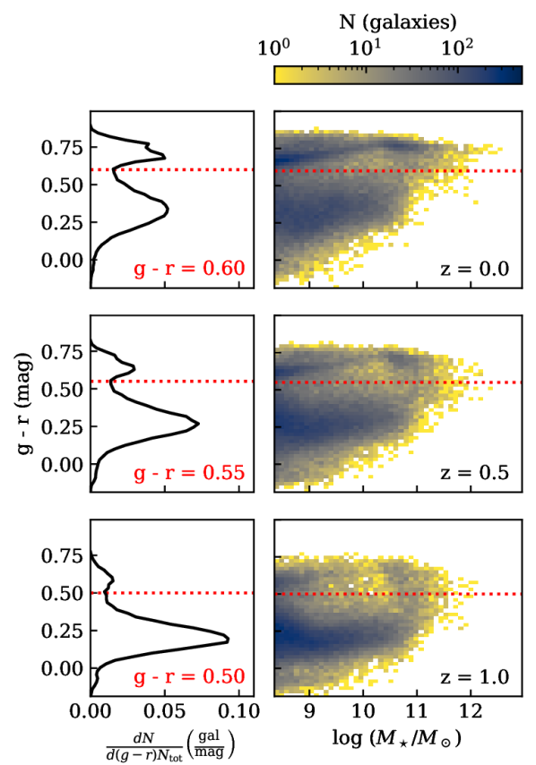
Figure 1: Distribution of galaxy colours in TNG100 at $z=0$ (top), $z=0.5$ (centre), and $z=1$ (bottom). 2D histograms (right) show the colour-$M_{\star}$ distribution. 1D colour distributions (left) sum along each $g\!$ - $\!r$ bin in the colour-$M_{\star}$ plane, normalised by the number of galaxies at that redshift, $N_{\rm{tot}}$. The red dotted line represents the bin with the minimum galaxy count between the peaks of the bimodal distribution, chosen to be the threshold that separates galaxies into blue (below line) and red (above line) subpopulations. The blue cloud is distributed over a wide range of $g\!$ - $\!r$ values and reaches a maximum at $M_{\star}\approx 10^{11}M_{\odot}$. The red sequence has a tight $g\!$ - $\!r$ distribution with larger spread in $M_{\star}$.

We remove galaxies with $M_{\star}<2\times 10^{8}$ $\rm{M}_{\odot}$ as the data from galaxies with fewer than 100 stellar particles is unreliable. We then separate the galaxies into blue and red using the difference in magnitude in the g- and r-bands, as defined by the Sloan Digital Sky Survey (SDSS, Stoughton et al., 2002). The resulting colour$-M_{\star}$ plane is shown in Fig. 1. For each redshift, we select the $g\!$ - $\!r$ value that corresponds to the bin with the minimum count between the two peaks in the colour distribution. Galaxies falling on or above the line are classified as blue and all others as red. We find that the minimum evolves from $g\!$ - $\!r$ = 0.60, $g\!$ - $\!r$ = 0.55, and $g\!$ - $\!r$ = 0.50 at $z=0$, $z=0.5$, and $z=1$, respectively. Nelson et al. (2018) find that IllustrisTNG’s $g\!$ - $\!r$ distribution roughly matches observations in our redshift range.

However, at high redshift ($z>1$) IllustrisTNG’s colour distribution begins to diverge from observations. IllustrisTNG lacks dusty and star-forming red galaxies (Donnari et al., 2019), an observed phenomenon that is also missing in other simulations such as MUFASA (Davé et al., 2017). Only recently has the follow-up simulation for MUFASA, SIMBA (Davé et al., 2019), produced this population (Akins et al., 2022). We use redshifts $z\leq 1.0$ where the star-forming red population is negligible in IllustrisTNG (online figures), such that nearly all red galaxies are quenched and blue galaxies star-forming. We test the sensitivity of the blue and red galaxy clustering to different $g\!$ - $\!r$ thresholds and the effect of dust reddening according to the model from Nelson et al. (2018). The clustering of both blue and red galaxies is not appreciably impacted by any reasonably chosen colour threshold or by dust reddening (see Appendix A).

2.2 Modelling atomic and molecular hydrogen

We adopt the same notation as Diemer et al. (2018) to distinguish between the states of hydrogen, involving a consistent set of subscripts for any physical quantity that would be associated with the gas. If $\Sigma$ is the surface density, then $\Sigma_{\rm{gas}}$ is adopted for all gas, $\Sigma_{\rm{H}}$ for all hydrogen, $\Sigma_{\rm{HI+H}_{2}}$ for neutral hydrogen, $\Sigma_{\rm{HI}}$ for atomic hydrogen, and $\Sigma_{\rm{H}_{2}}$ for molecular hydrogen. Using this notation, the molecular fraction is defined as

$$f_{\rm{mol}}=\frac{M_{\rm{H}_{2}}}{M_{\rm{HI}+\rm{H}_{2}}}\,.$$ (1)

Equation 1 provides just one of the necessary ingredients to compute $M_{\mathrm{HI}}$ for each gas cell. We also require the fraction of gas that is hydrogen, $f_{\rm{H}}=M_{\rm{H}}/M_{\rm{gas}}$, and the fraction of hydrogen that is neutral, $f_{\rm{HI+H}_{2}}=M_{\rm{HI}+\rm{H}_{2}}/M_{\rm{H}}$. With these definitions, we can describe the mass of ${\rm H}$ i within a gas cell as

$$M_{\rm{HI}}=(1-f_{\rm{mol}})\times f_{\rm{HI+H}_{2}}\times f_{\rm{H}}\times M_{\rm{gas}}\,.$$ (2)

IllustrisTNG provides $f_{\rm{H}}$ and $f_{\rm{HI+H}_{2}}$ by tracking the abundance of hydrogen, helium and a small network of metals among other physical processes (Faucher-Giguère et al., 2009; Vogelsberger et al., 2013; Rahmati et al., 2013; Ferland et al., 2017; Pillepich et al., 2018a).

However, in star-forming cells, $f_{\rm{HI+H}_{2}}$ is not computed self-consistently in the IllustrisTNG model (Springel & Hernquist, 2003) and is thus treated separately. Star-forming cells are divided into a hot and cold gas phase. The entire hot phase is assumed to be ionized, and any ionization due to local young stars is neglected in the cold phase, yielding $f_{\rm{HI}+\rm{H}_{2}}=f_{\rm{H}}\rho_{\rm{cold}}/\rho_{\rm{gas}}$. A more detailed discussion of this assumption can also be found in Vogelsberger et al. (2013) and Diemer et al. (2018).

To model the final ingredient, $f_{\rm{mol}}$, we must post-process the simulation because IllustrisTNG does not distinguish between molecular and atomic hydrogen. Physically, $f_{\rm{mol}}$ is the result of a balance between H₂ production on dust grains and photo-dissociation via Lyman-Werner radiation. Thus $f_{\rm{mol}}$ models require the gas metallicity, gas surface density, and the intensity of incident UV radiation in the Lyman-Werner band as input (Draine, 2011). We must post-process the simulation to estimate the incident Lyman-Werner UV flux on a particular gas cell because IllustrisTNG does not include radiative transfer. The UV flux on any cell originates from two sources: the cosmological UV background (Faucher-Giguère et al., 2009) and from nearby star-forming regions. The incident UV flux on gas in galaxies is dominated by nearby stars. The gas in filaments, however, receives significant UV flux from distant sources. However, radiative transfer across the entirety of the simulation volume is impractical. We employ models with two approaches to resolve the filamentary gas issue: Villaescusa-Navarro et al. (2018), which neglects stellar UV sources, and Diemer et al. (2018), which neglects gas in filaments. We will briefly describe the relevant portions of each of the two approaches; for more details see the discussed papers.

Villaescusa-Navarro et al. (2018, hereafter VN18) treats star-forming and non-star-forming gas cells separately. VN18 assigns $f_{\rm{mol}}=0$ in non-star-forming gas, neglecting the trace amounts of H₂. For star-forming gas, $f_{\rm{mol}}$ is calculated using the Krumholz, McKee, & Tumlinson (KMT) model (Krumholz et al., 2008, 2009). KMT estimates $f_{\rm{mol}}$ when given properties characterizing the cloud’s size, metallicity, and the intensity of the photo-dissociating UV radiation in the Lyman-Werner band (Krumholz et al., 2008). VN18 neglects photo-dissociating UV radiation from local star formation, only incorporating background UV estimates from IllustrisTNG itself (Faucher-Giguère et al., 2009).

Diemer et al. (2018, hereafter D18) utilize five models of three different types to compute $f_{\rm{mol}}$: models based on observed correlations (Leroy et al., 2008), calibrations with simulations (Gnedin & Kravtsov, 2011; Gnedin & Draine, 2014), and analytical models (Krumholz, 2013; Sternberg et al., 2014). These models require the same three inputs as the model from VN18: the gas metallicity, density, and the incident UV intensity in the Lyman-Werner band. D18 use the SFR of nearby cells to approximate incident UV from local stellar sources, assuming an optically thin medium (see Gebek et al. (2023) for comparison to full radiative transfer prescriptions). The models used by D18 are tuned for 2D surface densities, not the 3D densities from the simulation. D18 convert from 3D to 2D in two ways: a cell-by-cell method using the Jean’s length and by projecting the galaxy in a face-on orientation onto a 2D grid of pixels (see their section 2.3). Each of the five $f_{\rm{mol}}$ models is then applied to the 2D quantities, except Leroy et al. (2008) which yields unphysical results when applied cell-by-cell. In total, this procedure results in nine ${\rm H}$ i distributions from D18.

2.3 Power spectra

We compute the power spectra of the overdensity $\delta(\boldsymbol{x})=\rho(\boldsymbol{x})/\overline{\rho}-1$ with

$$\langle\tilde{\delta}_{i}(\boldsymbol{k})\tilde{\delta}_{j}(\boldsymbol{k}^{\prime})\rangle=(2\pi)^{3}P_{i\times j}(k)\delta_{D}^{3}(\boldsymbol{k}-\boldsymbol{k}^{\prime})\,.$$ (3)

$P_{i\times j}(k)$ is the power spectrum and $\boldsymbol{k}$ is the wavenumber, with bold denoting a vector. $\delta_{D}$ is the Dirac delta function. $\tilde{\delta_{i}}$ represents the Fourier transform of the overdensity from position-space to $k$-space. If $i=j$ in the above equation, $P_{i\times j}(k)$ is called an auto power spectrum, which will be denoted with one population $P_{i}(k)$. Otherwise, it is called a cross-power spectrum.

The halo occupation distribution (Peacock & Smith, 2000; Berlind & Weinberg, 2002; Kravtsov et al., 2004; Tinker et al., 2005; Zheng et al., 2007; Hadzhiyska et al., 2020) provides a useful analytical framework for understanding power spectra. We can represent the power spectrum as a sum of contributions of inter- and intra-halo galaxy pairs,

$$P(k)=P^{2\rm{h}}(k)+P^{1\rm{h}}(k)+P^{\rm{SN}}\,.$$ (4)

The two-halo term reflects large-scale structure and the one-halo term structure within haloes. The shot noise term is a constant determined by the size of the sample used to measure the clustering. In the following sections, we will often refer to this framework to guide our analysis of the power spectra.

We consider power spectra in both real and redshift space. Matter is placed in redshift space $\boldsymbol{s}$ by displacing real-space positions along an arbitrarily chosen line-of-sight using their velocities,

$$\boldsymbol{s}=\boldsymbol{x}+\frac{1+z}{H(z)}\boldsymbol{v_{\parallel}}(\boldsymbol{r})\,,$$ (5)

where $H(z)$ is the Hubble parameter, $\boldsymbol{x}$ is position in real space, and $\boldsymbol{v_{\parallel}}$ is the velocity parallel to the chosen line of sight. The resulting real- and redshift-space matter distributions are placed in a $800^{3}$ grid with bin lengths of $\approx$ 95 h^-1 ckpc, binned using a Cloud-In-Cell (CIC) interpolation scheme. The grids are then used as input for the power spectrum calculation routine provided by the Python library Pylians (Villaescusa-Navarro, 2018). Our results are converged with grid resolution at all relevant scales (online figures).

We can quantify the “faithfulness” of a matter tracer using the bias $b_{ij}(k)=\tilde{\delta_{i}}(\boldsymbol{k})/\tilde{\delta_{j}}(\boldsymbol{k})$, where $i$ and $j$ represent two different populations. For this paper, we are exclusively interested in the bias of matter tracers with respect to the full mass distribution, so we always take $j$ to mean “all matter” and express the bias as $b_{i}$. We calculate the bias as

$$P_{i}(k)=b_{i}^{2}(k)P_{\rm{m}}(k)\,$$ (6)

where $P_{\rm{m}}$ is the matter power spectrum, and $i$ represents some chosen matter tracer such as ${\rm H}$ i or galaxies.

To measure the strength of the relationship between two samples, we use the correlation coefficient

$$r_{i-j}=\frac{P_{i\times j}(k)}{\sqrt{P_{i}(k)P_{j}(k)}}\,.$$ (7)

$r_{i-j}$ takes a value of zero for completely random distributions and approaches unity for entirely dependent samples. We distinguish the correlation coefficient from the position vector by denoting the vector $\boldsymbol{r}$ using a bold letter and the length scale $R$ with a capital.

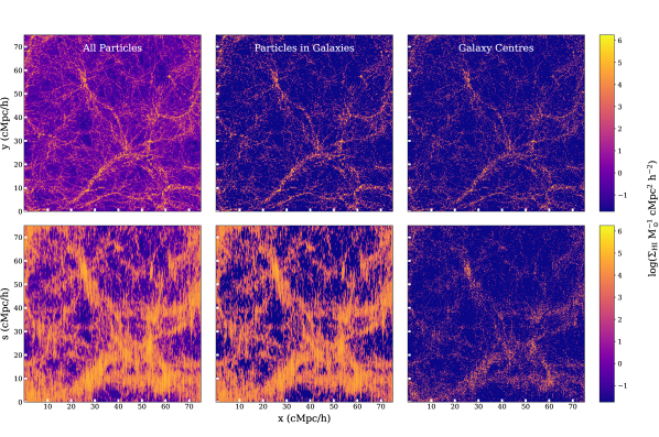
Figure 2: Slices through the IllustrisTNG ${\rm H}$ i mass distribution at $z=0$ in real (top) and redshift space (bottom). Each slice sums 20% of the simulation volume along the $z$-axis. The redshift-space distributions are created by displacing particles from their positions in real space using their velocities along the line of sight, in this case the $y$-axis. The left column shows the model of VN18, which calculates the ${\rm H}$ i in all gas cells but does not account for local UV sources, whereas the remaining distributions account for local UV sources but only account for gas cells within galaxies. The middle and right columns display ${\rm H}$ i distributions calculated by D18 with the Gnedin & Draine (2014) model, using the positions of individual gas cells and the centre of the host galaxy, respectively. The sizes of the points in the right column scale logarithmically with galaxy ${\rm H}$ i mass. In the bottom row, the fingers-of-God effect can be observed in all three cases. In the Galaxy Centres case, however, the fingers-of-God manifest more weakly because it removes the contribution of the velocities of the cells within a galaxy along the line of sight.

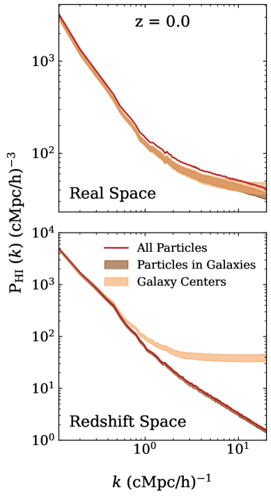
Figure 3: ${\rm H}$ i auto power spectra in real (top) and redshift space (bottom) at $z=0$. The contours delineate the models from D18 that are applied to galaxies as a whole (light brown, nine models) and to the individual particles within galaxies (dark brown, four models). The crimson line represents the distribution from VN18. All distributions are similar in real space, although All Particles receives a small boost by including filaments. In redshift space, Galaxy Centres diverges from the other auto powers at $k\sim 0.5$ h cMpc^-1. Representing galaxies as points removes any velocity contributions from individual gas cells, tempering the fingers-of-God effect. We represent subsequent ${\rm H}$ i power spectra using shaded areas encompassing each model.

3 Results

In this section, we characterize the clustering of ${\rm H}$ i, blue, and red galaxies. In Section 3.1, we show that the ${\rm H}$ i distribution is not particularly sensitive to the post-processing of the simulations. We analyse how ${\rm H}$ i clusters with different galaxy samples separated by colour in Section 3.2 and examine their scale- and time-dependence in Section 3.3. We study how the cross-power spectra change as a function of $M_{\star}$ in Section 3.4 and $M_{\mathrm{HI}}$ in Section 3.5. In Appendix B, we show how simulation resolution affects these results.

3.1 Hi auto power spectra

Before we proceed, we must ascertain if our results are sensitive to the post-processing models used to calculate ${\rm H}$ i distributions in IllustrisTNG. We split the ${\rm H}$ i models into three groups: Galaxy Centres, Particles in Galaxies, and All Particles. For models in Galaxy Centres, we assign all the ${\rm H}$ i in a galaxy to its centre for all nine models from D18. The four cell-by-cell models from D18 are also included in the next group, Particles in Galaxies, where we instead assign ${\rm H}$ i to the position of each individual host cell. Gas cells outside of galaxies are excluded in both cases (Section 2.2). For the final group, All Particles, we apply the one model from VN18 to every gas cell in the simulation. In this section, we compare the ${\rm H}$ i clustering for the ${\rm H}$ i models in and amongst these three groups.

We show slices through the real-space ${\rm H}$ i distributions in the top row of Fig. 2 to provide insight into the ${\rm H}$ i auto power spectra in the top panel of Fig. 3. The filaments present in All Particles (top left in Fig. 2) but missing in Galaxy Centres and Particles in Galaxies (top middle and right, respectively) reflect the trade-off described in Section 2.2 – namely, the neglect of local UV sources in VN18 and of filaments in D18. The filaments that connect galaxies supply some small mass-weighted power to all scales in between them, boosting the ${\rm H}$ i power spectrum from All Particles slightly in Fig. 3. On small scales, Galaxy Centres diverges from Particles in Galaxies, as representing a galaxy’s ${\rm H}$ i as a point removes any clustering within galaxies. For all power spectra presented in this work, we exclude scales below $k\approx 20$ h cMpc^-1 due to aliasing issues near the Nyquist frequency ($k_{\rm{Nyq}}=33$ h cMpc^-1).

Measurements of ${\rm H}$ i, however, take place in redshift space. Line-of-sight velocities distort the real-space power spectra primarily in two ways, called redshift-space distortions (RSD): the Kaiser effect (Kaiser, 1987) and fingers-of-God (FoG, Jackson, 1972). The Kaiser effect enhances each redshift-space auto power spectrum (bottom panel of Fig. 3) on large scales, as groups of galaxies moving coherently appear closer in redshift space. The second RSD, FoG, manifests due to the velocity dispersions within a halo, smearing the distribution on small scales into the columns (“fingers”) along the line of sight (bottom left and centre panels of Fig. 2). FoG suppress the redshift-space power spectrum compared to the real-space counterparts for each ${\rm H}$ i group (bottom of Fig. 3), although the magnitude of the suppression varies between groups.

FoG manifest more weakly in Galaxy Centres than in Particles in Galaxies and All Particles. The strength of FoG in each ${\rm H}$ i group is dependent on its velocity dispersion (Juszkiewicz et al., 2000). The velocity dispersion for Particles in Galaxies and All Particles receives contributions from the velocity dispersion of galaxies themselves and their constituent particles (Zhang et al., 2020). By collapsing ${\rm H}$ i to the centre of each galaxy, Galaxy Centres removes contributions from the intrinsic velocity dispersion of the particles within a galaxy, softening the net FoG in the Galaxy Centres case. As a result, the redshift-space ${\rm H}$ i auto power for Galaxy Centres breaks away from the other two groups at $k\gtrsim 0.5$ h cMpc^-1, before approaching a constant value due to shot noise at $k\sim 2$ h cMpc^-1.

In following sections, we represent ${\rm H}$ i power spectra as shaded areas encompassing results calculated from each of the ${\rm H}$ i models from all groups and treat the contours as systematic uncertainties due to ${\rm H}$ i post-processing. However, we exclude Galaxy Centres from redshift-space power spectra since their FoG are artificially suppressed.

3.2 Hi-Galaxy cross-power spectra

Previous works have established the environmental dependence of a galaxy’s gas abundance, finding that cluster members have significantly lower gas fractions (Giovanelli & Haynes, 1985; Solanes et al., 2002; Brown et al., 2021). We can measure the effect of this environmental dependence on larger scales by computing cross-power spectra between ${\rm H}$ i and blue galaxies (${\rm H}$ i $\times$ Blue) and ${\rm H}$ i and red galaxies (${\rm H}$ i $\times$ Red). In Section 3.2.1 we focus on their scale- and colour-dependence in real space. In Section 3.2.2, we study the impact of RSDs on those relationships.

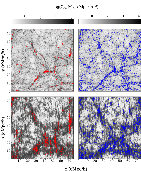
Figure 4: Slices of the red (left) and blue (right) galaxy distributions overlaid with the ${\rm H}$ i distribution from VN18. The slices show TNG100 at $z=0$, summing 20% of the $z$-plane centred in the middle of $z$-axis, in both real (top) and redshift (bottom) space. Matter was placed in redshift space by projecting its velocities along the line of sight, in this case the $y$-axis. Red galaxies are clearly more clustered, grouping heavily around the largest haloes, whereas the blue galaxies better trace out the ${\rm H}$ i distribution across the box.

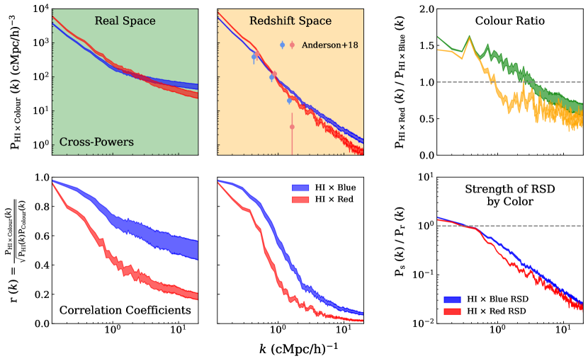
Figure 5: Cross-power spectra (top) and correlation coefficients (bottom) for ${\rm H}$ i $\times$ Red and ${\rm H}$ i $\times$ Blue at $z=0$ in real space (left, green) and redshift space (centre, yellow), shown as contours that enclose the ${\rm H}$ i models. The cross-power spectra are calculated with respect to the total ${\rm H}$ i distribution, not only the ${\rm H}$ i in galaxies of the respective colour. We compare the observational data from Anderson et al. (2018) to the redshift-space power spectra, displayed as points. For clarity, red points are offset in $k$. The point at which the cross-power spectra intersect is more discernible in the ratio ${\rm H}$ i $\times$ Red over ${\rm H}$ i $\times$ Blue (top right) for both real (green, $k_{\rm{eq}}\approx 3.25$ h cMpc^-1) and redshift space (yellow, $k_{\rm{eq}}\approx 0.9$ h cMpc^-1). We compare the ratio of redshift-space over real-space power spectra for ${\rm H}$ i $\times$ Red and ${\rm H}$ i $\times$ Blue (bottom right). At small scales, ${\rm H}$ i $\times$ Red is suppressed more than ${\rm H}$ i $\times$ Blue because FoG are stronger in red galaxies. This adds a secondary colour-dependency, which pushes the intersection between the cross-power spectra out to $\sim 10.4$ Mpc in redshift space. The correlation coefficients confirm that ${\rm H}$ i is more tightly linked to blue galaxies than red at all scales in both real and redshift space.

3.2.1 Real space

The top row of Fig. 4 shows the distribution of blue and red galaxies overlaid on ${\rm H}$ i in real space. Red galaxies (top left panel) are concentrated in the densest regions while blue galaxies (top right) are broadly distributed. Massive, older, and more clustered haloes tend to host red galaxies, leading to colour-dependent clustering and a larger bias (equation 6) with respect to matter for red galaxies than blue galaxies (Gao et al., 2005; Zehavi et al., 2005b; Wechsler et al., 2006; Springel et al., 2018). The intrinsic clustering strength of red galaxies manifests in the cross-power spectra shown in Fig. 5 via their larger bias. Mathematically, we can express the cross-power spectra as

$$P_{\mathrm{HI}\times\mathrm{Colour}}(k)=b_{\rm{HI}}(k)b_{\rm{Colour}}(k)r_{\rm{HI-Colour}}(k)P_{\rm{m}}(k)$$ (8)

to describe how they relate to the bias $b_{\rm{Colour}}$, correlation coefficient $r_{\rm{HI-Colour}}$, and matter power spectrum $P_{\rm{m}}$. Equation 8 is useful for understanding the galaxy properties responsible for the relative strengths of ${\rm H}$ i $\times$ Blue and ${\rm H}$ i $\times$ Red: their inherent clustering strength, represented by their bias $b_{\rm{Colour}}$, and their spatial relationship with ${\rm H}$ i, represented by the correlation coefficient $r_{\rm{HI-Colour}}$ (equation 7).

${\rm H}$ i $\times$ Red is greater than ${\rm H}$ i $\times$ Blue on large scales (Fig. 5) because red galaxies cluster more strongly ($b_{\rm{Red}}>b_{\rm{Blue}}$). However, this trend is counteracted by the weaker spatial connection between red galaxies and ${\rm H}$ i ($r_{\rm{HI-Red}}<r_{\rm{HI-Blue}}$, bottom row). The disparity between the correlation coefficients is small on large scales ($r_{\rm{HI-Red}}\approx r_{\rm{HI-Blue}}\approx 1$) because the clustering of ${\rm H}$ i is colour-independent, in the sense that its distribution is governed mostly by linear growth rather than small-scale effects. However, ${\rm H}$ i tends to be suppressed in the massive haloes hosting red galaxies, reducing $r_{\rm{HI-Red}}$ faster than $r_{\rm{HI-Blue}}$ when approaching small scales. The disparity between the correlation coefficients grows such that on small scales the ${\rm H}$ i $\times$ Blue cross-power spectrum is greater than ${\rm H}$ i $\times$ Red. We describe the clustering of ${\rm H}$ i on these scales as “colour-dependent” since the spatial relationship between ${\rm H}$ i and galaxies governs the relative strengths of each cross-power spectra more than the galaxy population’s inherent clustering.

In terms of equation 8, we can call those scales colour-independent when ${\rm H}$ i $\times$ Red is greater than ${\rm H}$ i $\times$ Blue, as $P_{\mathrm{HI}\times\mathrm{Red}}/P_{\mathrm{HI}\times\mathrm{Blue}}>1$ implies $b_{\rm{Red}}/b_{\rm{Blue}}>r_{\rm{HI-Blue}}/r_{\rm{HI-Red}}$ and therefore the intrinsic clustering of the galaxy population dictates the relative strengths of the cross-power spectra on large scales. On the other hand, colour-dependent scales occur when ${\rm H}$ i $\times$ Blue is greater than ${\rm H}$ i $\times$ Red, as $P_{\mathrm{HI}\times\mathrm{Red}}/P_{\mathrm{HI}\times\mathrm{Blue}}<1$ implies $b_{\rm{Red}}/b_{\rm{Blue}}<r_{\rm{HI-Blue}}/r_{\rm{HI-Red}}$, showing that the galaxy population’s spatial relationship with ${\rm H}$ i is largely responsible for their relative strengths. We roughly interpret the scale at which the intersection between ${\rm H}$ i $\times$ Red and ${\rm H}$ i $\times$ Blue occurs ($k_{\rm{eq}}$) as the transition between the colour-independent and -dependent regimes, but emphasize that $k_{\rm{eq}}$ is not a sharp transition.

The intersection is easily identifiable when the ratio of ${\rm H}$ i $\times$ Red over ${\rm H}$ i $\times$ Blue (top right panel of Fig. 5) falls below unity at $k_{\rm{eq}}\approx 3.25$ h cMpc^-1 ($R_{\mathrm{eq}}=2\pi/k_{\rm{eq}}\approx 2.8$ Mpc). The scale at which the ${\rm H}$ i distribution becomes significantly more colour-dependent reflects the findings of previous work on the concept of “galaxy conformity”. Galaxies within $\sim 4$ Mpc of a larger red galaxy tend to also be red (Kauffmann et al., 2013), indicating that a galaxy’s large-scale environment impacts its star-formation (Hearin et al., 2016; Ayromlou et al., 2023). Given the link between ${\rm H}$ i and star-formation (Bigiel et al., 2008), it is reasonable that the ${\rm H}$ i content of galaxies would also be suppressed within 4 Mpc of a large red galaxy. This crossover also matches the $z\approx 0$ cross-correlation between SDSS galaxies (York et al., 2000) and ALFALFA ${\rm H}$ i maps (Giovanelli et al., 2005; Haynes et al., 2011) from Papastergis et al. (2013), where they find that ${\rm H}$ i abundance is reduced within 3 Mpc ($k\sim 3.14$ h cMpc^-1) of a red galaxy. The agreement between IllustrisTNG and observations is encouraging.

3.2.2 Redshift space

Fig. 4 shows slices through the redshift-space distributions of red and blue galaxies overlaid on ${\rm H}$ i (bottom row), where the FoG in red galaxies stretch over longer distances than in blue galaxies (Li et al., 2006). The massive haloes that host red galaxies possess deep potential wells, causing a large velocity dispersion in the member galaxies that can stretch FoG for nearly half the length of the box. This colour-dependency in the strength of FoG alters the comparison between ${\rm H}$ i $\times$ Blue and ${\rm H}$ i $\times$ Red in the redshift-space cross-power spectra, which are provided in Fig. 5 (top middle panel).

We quantify the strength of RSDs on the power spectra with the ratio of real- and redshift-space power spectra (bottom right panel of Fig. 5). At large scales, the redshift-space power spectra are slightly greater than their real-space counterparts until $k\sim 0.4$ h cMpc^-1. The boost arises from the Kaiser effect (Section 3.1) and manifests similarly in both ${\rm H}$ i $\times$ Blue and ${\rm H}$ i $\times$ Red. Although both ${\rm H}$ i $\times$ Blue and ${\rm H}$ i $\times$ Red will approach the Kaiser limit at sufficiently large scales, it is unclear if they will approach the limit similarly, and it is difficult to extrapolate from the small $k$ regime that probes the Kaiser effect. At small scales, FoG dominate the distortion of redshift-space power spectra, reducing ${\rm H}$ i $\times$ Blue and ${\rm H}$ i $\times$ Red significantly within $k>0.4$ h cMpc^-1. FoG suppress ${\rm H}$ i $\times$ Red more strongly than ${\rm H}$ i $\times$ Blue, with the two diverging at $k\sim 0.5$ h cMpc^-1. The stronger FoG in ${\rm H}$ i $\times$ Red introduce a secondary colour-dependent effect in the redshift-space cross-power spectra. Consequently, the redshift-space colour ratio (top right panel of Fig. 5) curves downward much more rapidly at $k\approx 0.4$ h cMpc^-1 and reaches unity at a much larger scale in redshift-space ($R_{\mathrm{eq}}\approx 10.4$ Mpc) than in real space ($R_{\mathrm{eq}}\approx 2.8$ Mpc). At $k>1$ h cMpc^-1, random particle velocities emerge as noise in the redshift-space power spectra—this effect is small and does not alter any conclusions made in this paper.

Below the redshift-space cross-power spectra in Fig. 5, we showcase the $z=0$ redshift-space correlation coefficients. Similarly to their real-space counterparts, ${\rm H}$ i $\times$ Blue has a greater correlation coefficient than ${\rm H}$ i $\times$ Red at all scales. However, both ${\rm H}$ i $\times$ Red and ${\rm H}$ i $\times$ Blue decrease much more sharply at $k\sim 1$ h cMpc^-1 than in real-space, with their redshift-space correlation coefficients reaching $\sim 0.1$ on the smallest scales. We speculate that the spatial disconnect may arise from differences in velocity dispersions between ${\rm H}$ i and galaxies. ${\rm H}$ i possesses intrinsic velocity dispersion within galaxies (Zhang et al., 2020), whereas galaxies only experience pair-wise velocity dispersion. We reserve further analysis for the following paper (Osinga et al., in prep).

The power spectra shown in Fig. 5 agree with $z\sim 0$ observations. Anderson et al. (2018) computed cross-correlations between 2df galaxies (Colless et al., 2001) and Parkes ${\rm H}$ i maps (Staveley-Smith et al., 1996), shown as points in the top centre panel of Fig. 5. Our results match in the range $0.3<k<1.5$ h cMpc^-1, with both ${\rm H}$ i $\times$ Blue and ${\rm H}$ i $\times$ Red within their statistical uncertainties. We both find that ${\rm H}$ i $\times$ Red is greater on large scales but drops beneath ${\rm H}$ i $\times$ Blue at smaller scales, intersecting within $0.8<k<1.5$ h cMpc^-1 range. Anderson et al. (2018) measure ${\rm H}$ i suppression around red galaxies to much larger scales than Papastergis et al. (2013) ($\sim 10$ Mpc compared to $\sim 3$ Mpc) because of RSDs. Papastergis et al. (2013) employ a projected correlation function that measures clustering perpendicular to the line of sight, removing RSD effects. At larger scales $k\sim 0.1-0.3$ h cMpc^-1, Anderson et al. (2018) find anti-correlations between ${\rm H}$ i and galaxies, which we exclude from Fig. 5 due to their large uncertainties. Interestingly, other intensity mapping experiments find subdued (although still positive) ${\rm H}$ i clustering at similar scales even at other redshifts (Wolz et al., 2021; Paul et al., 2023), however we find no evidence for such behaviour in IllustrisTNG.

3.3 Redshift evolution

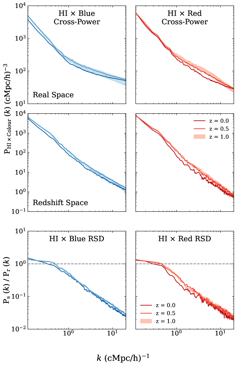
Figure 6: Redshift evolution of ${\rm H}$ i $\times$ Blue (left) and ${\rm H}$ i $\times$ Red (right) in real (top) and redshift (centre) space for $z=0,0.5$, and 1 (darkest to lightest colour). The bottom row shows the redshift evolution of the ratio of redshift-space over real-space power spectra, measuring the strength of RSDs. For clarity, we only plot the contour with all ${\rm H}$ i models for $z=1$ and plot the others as a line representing the contour’s centre—the width of the contours does not change significantly across redshift. In real and redshift space, both cross-power spectra either change little or decrease with time. These trends seem to conflict with the picture of structure growth but occur due to colour transitions and gas loss (see text). For each colour, RSDs strengthen slightly with time, amplifying the loss of clustering at later times in redshift space as compared to real space.

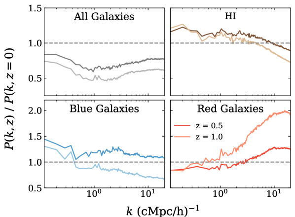
Figure 7: Redshift evolution of the all-galaxy (top left), ${\rm H}$ i (top right), blue galaxy (bottom left), and red galaxy (bottom right) auto power spectra in real space divided by the $z=0$ auto power spectra. Darker colours indicate results closer to $z=0$. The ${\rm H}$ i auto powers are displayed using the centre of the contour containing all the ${\rm H}$ i models. The only auto power that consistently increases with time is the galaxy auto power spectrum. This implies that the decrease in the clustering of red and blue galaxies with time arises due to colour transitions.

Assuming that gravity is the dominant influence on the time evolution of power spectra, we expect the clustering of matter to increase linearly on large scales with respect to the growth factor and non-linearly on small scales (Fry, 1996; Dodelson & Schmidt, 2020). However, the behaviour of ${\rm H}$ i $\times$ Blue and ${\rm H}$ i $\times$ Red in Fig. 6 deviates from those expectations. From $z=1$ to $z=0.5$, ${\rm H}$ i $\times$ Blue and ${\rm H}$ i $\times$ Red experience negligible changes and from $z=0.5$ to $z=0$ their power spectra even diminish with time. This discrepancy prompts us to investigate the various processes responsible for the time evolution of each cross-power spectrum. Since cross-power spectra conflate changes in the member distributions and their spatial relationship (Section 3.2), we analyse the auto power spectra of the member distributions first in Fig. 7 and then apply those insights to the ${\rm H}$ i-galaxy cross-power spectra.

Throughout this section, we examine three interconnected processes that shape the redshift evolution of power spectra: galaxy quenching, gas loss, and colour transitions. While these processes are certainly linked, it is important to clarify their precise meanings in our analysis. We employ the term “quenching” to describe galaxies leaving the star-formation main sequence (Daddi et al., 2007; Noeske et al., 2007; Donnari et al., 2019). “Gas loss” refers to processes that strictly affect ${\rm H}$ i clustering by reducing a galaxy’s gas reservoirs, regardless of when the gas loss occurs relative to quenching. A “colour transition” denotes a galaxy’s transition from blue to red along the $g\!$ - $\!r$ axis, again independent of quenching. Galaxy quenching, per these definitions, is largely not responsible for the redshift evolution of the power spectra, but it is closely associated with other two processes that do contribute to this trend. For the remainder of the paper, we refer to quenching, gas loss, and colour transitions with these definitions in mind.

The bottom row of Fig. 7 shows that both the blue and red galaxy auto power spectra decrease with time from $z=1$ to $z=0$, despite the all-galaxies auto power spectrum (top left panel) continuing to grow. This discrepancy implies that the decreasing auto power spectra for both blue and red galaxies is an artefact of making a colour cut. Some fraction of galaxies transition from blue to red between redshifts. These transitioning galaxies tend to be the “reddest,” oldest, and most clustered members of the blue population. As a result, the average clustering of the remaining blue galaxies decreases upon losing their most clustered component (bottom left panel). Simultaneously, transitioning galaxies join the red population as its least clustered members, thereby reducing the average clustering of the red galaxies and decreasing their power spectrum (bottom right panel). The transitioning population at $z\leq 1$ is large enough to offset structure growth, particularly for red galaxies between $z=1$ and $z=0.5$ and blue galaxies between $z=0.5$ and $z=0$ when their smaller populations increase sensitivity to transitioning galaxies (Fig. 1). Importantly, it should be noted that this is not a result of moving the $g\!$ - $\!r$ cut with time (Section 2); these trends are amplified if the colour cut remains constant.

As of yet, the effect of colour transitions on the clustering evolution of ${\rm H}$ i and galaxies has not yet been properly understood. Previous observational studies on this subject focus on red galaxies (Zehavi et al., 2005a; White et al., 2007; Guo et al., 2013), as it is challenging to obtain complete samples of blue galaxies at higher redshifts (Wang et al., 2021). These studies have found that red galaxy clustering grows at a slower rate than all-galaxy clustering over $0\lesssim z\lesssim 1$, a phenomenon attributed to mergers and disruptions. However, our findings suggest that colour transitions are largely responsible for suppressing the clustering growth of blue and red galaxies. Blue galaxies merge at a slower rate than red galaxies (Lin et al., 2008; Darg et al., 2010), meaning that mergers and disruptions are unlikely to induce similar effects on the redshift evolution of the blue galaxy auto power spectrum (bottom left panel of Fig. 7). We will further discuss the contributions from mergers, disruptions, and colour transitions on the time evolution of the power spectra at different scales in Section 4.

In addition to the changes in the clustering of blue and red galaxies, the time evolution of ${\rm H}$ i $\times$ Blue and ${\rm H}$ i $\times$ Red is influenced by the behaviour of ${\rm H}$ i clustering. The upper right panel of Fig. 7 shows that the ${\rm H}$ i auto power spectrum increases between $z=1$ and $z=0.5$ before decreasing between $z=0.5$ and $z=0$. Given the connection between blue galaxies and ${\rm H}$ i, we speculate that the gas loss associated with colour transitions plays a significant role in the loss of structure from $z=0.5$ to $z=0$. Notably, the cosmic abundance of ${\rm H}$ i increases from $z=1$ to $z=0$ in IllustrisTNG (Villaescusa-Navarro et al., 2018; Diemer et al., 2019), which would seem to contradict our finding that the clustering decreases with time. This may be because of changes in the clustering of ${\rm H}$ i as a function of halo mass, however further investigations of this conflict are left to future work.

The redshift-space power spectra evolve with time similarly to their real-space counterparts. The strength of this trend is amplified in redshift space by the evolution of RSDs (bottom row of Fig. 6). For both colours, the RSDs suppress the redshift-space power spectra more strongly at later redshifts, albeit the relative weak evolution of the RSDs overall. Although not explicitly visible in Fig. 6, the redshift-space intersection between ${\rm H}$ i $\times$ Blue and ${\rm H}$ i $\times$ Red occurs at $R_{\mathrm{eq}}\approx 10.4,5.4$, and 3.8 Mpc at $z=0$, 0.5, and 1, respectively. These intersections at $z=0$ and $z=1$ are comparable to those reported by Anderson et al. (2018) and Wolz et al. (2021), respectively.

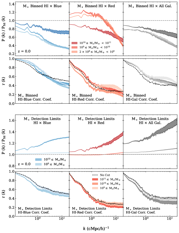
Figure 8: The clustering of stellar mass subsamples for ${\rm H}$ i $\times$ Blue (left), ${\rm H}$ i $\times$ Red (centre), and ${\rm H}$ i $\times$ Galaxy (right) in real space at $z=0$. Contours encompass all ${\rm H}$ i models, with darker colours representing subsamples with greater $M_{\star}$. The cross-power spectra for $M_{\star}$ bins (first row) and detection limits (third row) are shown as a ratio to the overall fiducial sample for that galaxy colour. ${\rm H}$ i $\times$ Blue and ${\rm H}$ i $\times$ Galaxy both cluster more with increasing $M_{\star}$. ${\rm H}$ i $\times$ Red, however, clusters the most weakly in the largest mass bin (see text for discussion). The correlation coefficients for each galaxy colour and ${\rm H}$ i (second row) evolve little with $M_{\star}$, demonstrating that differences in the cross-power spectra arise from changes in the clustering of the galaxy population rather than their spatial connection with ${\rm H}$ i. In the bottom two rows, we display cross-power spectrum ratios and correlation coefficients for galaxy samples above certain $M_{\star}$ thresholds, which represent a rough proxy for detection limits. ${\rm H}$ i $\times$ Red and ${\rm H}$ i $\times$ Galaxy converge to their fiducial cross-power with no (additional) mass cuts by $M_{\star}=10^{10}M_{\odot}$ and ${\rm H}$ i $\times$ Blue by $M_{\star}=10^{9}M_{\odot}$. ${\rm H}$ i $\times$ Blue converges at greater masses, as most galaxies in $M_{\star}\gtrsim 10^{10.5}M_{\odot}$ are red. We exclude the $M_{\star}\geq 10^{11}M_{\odot}$ threshold for ${\rm H}$ i $\times$ Blue, as it is dominated by shot noise.

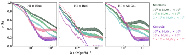
Figure 9: Correlation coefficients between ${\rm H}$ i and three galaxy colour populations, blue (left), red (middle), and all galaxies (right) at $z=0$. Each galaxy colour population is separated into stellar mass bins of width $\approx 1$ dex, with lighter colours representing less massive bins and darker more massive. Each stellar mass bin is further separated into centrals (purple) and satellites (green). ${\rm H}$ i correlates more strongly with satellites for increasing $M_{\star}$ across galaxy colour, but this trend reverses for centrals. By definition, there is only one central galaxy per halo, thus the correlation coefficients for centrals are constant on small scales.

3.4 Dependence on stellar mass in centrals and satellites

It is well-established that more luminous or massive galaxies cluster more strongly (Zehavi et al., 2005b, 2011; Beutler et al., 2013; Guo et al., 2013, 2014; Skibba et al., 2014; Zhai et al., 2023). In this section, we examine how this relationship manifests in cross-correlations with ${\rm H}$ i and test whether the tendency for observations to detect bright objects skews the measured cross-power spectra. We compare the clustering of galaxies whose stellar masses fall within three coarse $M_{\star}$ bins, as well as those whose stellar mass exceeds three lower detection limits with separations of $\approx 1$ dex. The $M_{\star}$ relationships of the cross-power spectra evolve little with redshift; for brevity, we examine only $z=0$ results and provide similar analyses at other redshifts in the online figures.

In the top row of Fig. 8, we separate blue, red, and all galaxies into coarse $M_{\star}$ bins and compute their cross-power spectra and correlation coefficients with ${\rm H}$ i. The correlation coefficients distinguish changes in the spatial connection of the galaxy subsample to ${\rm H}$ i from changes to the intrinsic clustering of the member distributions of the cross-power spectra (Section 3.2). Both ${\rm H}$ i $\times$ Blue (left column) and ${\rm H}$ i $\times$ Galaxy (right) increase with $M_{\star}$, showing that more massive galaxies in the blue and whole galaxy samples cluster more strongly. ${\rm H}$ i $\times$ Red (middle) on the other hand does not exhibit a clear trend with $M_{\star}$; we will elaborate on this behaviour later in the section.

The correlation coefficients (second row) for all galaxy colours vary negligibly with $M_{\star}$. This lack of evolution implies that within each $M_{\star}$ bin, the correlation between blue or red galaxies and ${\rm H}$ i does not significantly differ from that of other galaxies of the same colour but with different masses. Consequently, the $M_{\star}$ evolution of the cross-power spectra in the top row of Fig. 8 reflects the inherently stronger clustering of massive galaxies.

In addition to $M_{\star}$ bins, we also investigate cross-power spectra and correlation coefficients for lower $M_{\star}$ thresholds in Fig. 8, which we consider a rough analogue for detection limits in observations. The cross-power spectra for ${\rm H}$ i $\times$ Red and ${\rm H}$ i $\times$ Galaxy converge to the fiducial cross-power spectrum for the whole sample at $M_{\star}=10^{10}M_{\odot}$, and ${\rm H}$ i $\times$ Blue does the same at $M_{\star}=10^{9}M_{\odot}$. ${\rm H}$ i-galaxy cross-power spectra measured in observations with galaxy surveys complete up to those masses should be therefore insensitive to detection limits. The correlation coefficients for each $M_{\star}$ detection limit also converge to the fiducial sample by the same masses as the cross-power spectra for each colour.

The clustering of blue and all-galaxies in Fig. 8 increases with $M_{\star}$. Red galaxy clustering, however, only increases slightly from $2\times 10^{8}\leq M_{\star}/M_{\odot}<10^{9}$ to $10^{9}\leq M_{\star}/M_{\odot}<10^{10}$, before decreasing drastically in the largest $M_{\star}$ bin. This trend aligns with observations and previous simulation work, where the red galaxy auto power spectrum decreases in the range $10^{8.5}\lesssim M_{\star}/M_{\odot}\lesssim 10^{10}$ before increasing in $10^{10}\lesssim M_{\star}/M_{\odot}\lesssim 10^{11.5}$ (Zehavi et al., 2005b; Guo et al., 2011; Henriques et al., 2017; Springel et al., 2018). This unique trend is tied to the composition of each $M_{\star}$ bin with respect to centrals and satellites. The greatest $M_{\star}$ bin predominantly consists of centrals, whereas the two smallest mass bins are composed almost entirely of satellites. Central galaxies, by definition, must inhabit different haloes whereas satellites have no such restriction. As a result, a larger proportion of red galaxies in the smallest $M_{\star}$ bins reside in the same haloes, increasing their clustering.

To investigate the effect of central/satellite demographics on the $M_{\star}$ evolution, we analyse the ${\rm H}$ i correlation coefficients of blue, red, and all-galaxies split into centrals and satellites in Fig. 9. ${\rm H}$ i $\times$ Galaxy (right panel) correlation coefficients for centrals inherit their shape from ${\rm H}$ i $\times$ Blue (left), as most centrals are blue. Similarly, most satellites are red, such that satellite correlation coefficients for ${\rm H}$ i $\times$ Galaxy echo ${\rm H}$ i $\times$ Red. However, blue satellites boost the corresponding ${\rm H}$ i $\times$ Galaxy coefficients by contributing some correlations with ${\rm H}$ i. Central correlation coefficients (purple contours) approach constant values in the one-halo regime ($k\sim 0.3$ h cMpc^-1) because only one central can occupy each halo.

For all galaxy populations, satellites correlate more with ${\rm H}$ i with increasing $M_{\star}$ whereas centrals correlate less. We can interpret these correlations by understanding the influence of environment on a galaxy’s gas abundance. Various external processes increase in strength and frequency with environmental density (Brown et al., 2021; Zabel et al., 2022; Villanueva et al., 2022; Watts et al., 2023), such as starvation (Larson et al., 1980; van de Voort et al., 2017), ram pressure stripping (Gunn & Gott, 1972; Abadi et al., 1999), and gas heating via satellite-satellite interactions (Moore et al., 1996; Moore et al., 1998), among others. Larger central galaxies tend to occupy denser haloes that are more effective at removing gas, and thus central galaxies correlate less with ${\rm H}$ i with increasing $M_{\star}$ in the one-halo regime. Massive red centrals in particular (centre panel of Fig. 9) are nearly completely uncorrelated with ${\rm H}$ i out to $k\approx 3$ h cMpc^-1, or $R=2\pi/k\approx 2.1$ h^-1 cMpc, demonstrating the efficacy of external quenching mechanisms near the centres of massive haloes (Gómez et al., 2003; Balogh et al., 2004; Wolf et al., 2009; Woo et al., 2013).

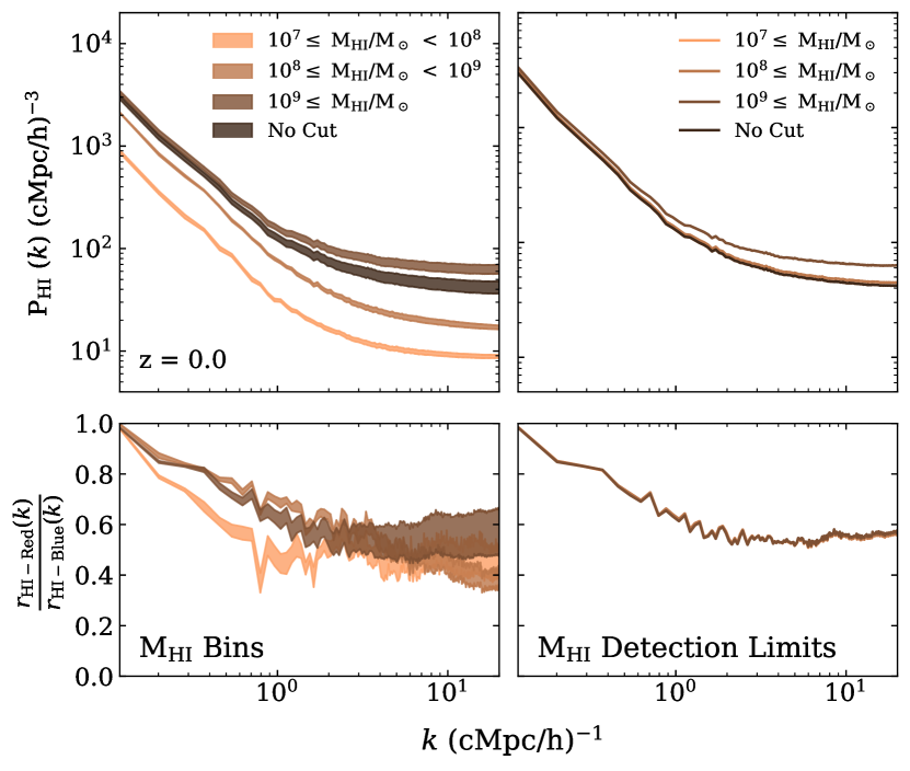
Figure 10: ${\rm H}$ i auto power spectra of galaxies within a particular $M_{\mathrm{HI}}$ subsample at $z=0$. For $M_{\mathrm{HI}}$ detection limits, we display only the centre of each contour encompassing the ${\rm H}$ i models to avoid crowding the figure. Breaking up the galaxy population into $M_{\mathrm{HI}}$ bins (top left), we find that the ${\rm H}$ i auto power grows with increasing $M_{\mathrm{HI}}$ (darker shades). The proximity of the fiducial ${\rm H}$ i auto power spectrum (black) to the largest $M_{\mathrm{HI}}$ bin implies that high $M_{\mathrm{HI}}$ galaxies dominate ${\rm H}$ i clustering. The similar auto power spectra for different $M_{\mathrm{HI}}$ thresholds (top right) demonstrate that the ${\rm H}$ i auto power is insensitive to detection limits. We examine the influence of the colour make-up of each $M_{\mathrm{HI}}$ subsample by providing the correlation coefficient ratio between an $M_{\mathrm{HI}}$ bin/threshold and all red galaxies over blue galaxies. A smaller $r$ ratio indicates that the galaxies within particular $M_{\mathrm{HI}}$ bin/threshold correlate more with blue galaxies than other $M_{\mathrm{HI}}$ bins/thresholds. The similar $r$ ratios across $M_{\mathrm{HI}}$ subsamples indicate that these trends do not arise from evolving galaxy colour demographics but instead from the inherent clustering strength of galaxies with greater $M_{\mathrm{HI}}$.

In contrast to centrals, satellite galaxies correlate more with ${\rm H}$ i with increasing $M_{\star}$. The reason for this trend is relatively straightforward for blue satellites. Massive blue satellites tend to inhabit larger ${\rm H}$ i-rich haloes, resulting in stronger ${\rm H}$ i correlations. On the other hand, the largest red satellites are typically hosted by haloes that are increasingly ${\rm H}$ i-deficient at larger masses, as indicated by their low $M_{\mathrm{HI}}/M_{h}$ (see figure 4 in Villaescusa-Navarro et al., 2018). This characteristic should lead to a decrease in the correlation between red satellites and ${\rm H}$ i at higher $M_{\star}$, which we do not find in Fig. 9. We speculate that this discrepancy may arise from two effects: satellite-satellite correlations and resistance to environmental effects. Satellites in massive haloes are, relative to the rest of the halo, ${\rm H}$ i-rich (see figure 7 in Villaescusa-Navarro et al., 2018). Larger haloes contain a greater number of satellites, which may mitigate their ${\rm H}$ i deficiency. The second effect, environment resistance, may also contribute as massive satellites possess deeper potential wells that can better withstand environmental stripping mechanisms (Marasco et al., 2016; Stevens et al., 2019; Donnari et al., 2021a).

3.5 Dependence on galaxy Hi mass

In the previous section, we studied how the ${\rm H}$ i-galaxy cross-power spectra evolve with $M_{\star}$. Here, we present a similar analysis with $M_{\mathrm{HI}}$. Observations have reached different conclusions about the behaviour of galaxy clustering with $M_{\mathrm{HI}}$. For example, Basilakos et al. (2007) and Guo et al. (2017) claim that the ${\rm H}$ i auto power spectrum increases as a function of $M_{\mathrm{HI}}$, while Meyer et al. (2007) and Papastergis et al. (2013) find no conclusive evidence of such a trend. We investigate this relationship in IllustrisTNG by separating galaxies at $z=0$ into three coarse $M_{\mathrm{HI}}$ bins and thresholds separated by 1 dex, and measure the clustering and correlation strength with blue and red galaxies for each $M_{\mathrm{HI}}$ subsample in Fig. 10.

We find that galaxy clustering increases as a function of $M_{\mathrm{HI}}$ in the top left panel of Fig. 10, supporting the conclusions of Basilakos et al. (2007) and Guo et al. (2017). In the bottom row, we show the ratio of the ${\rm H}$ i-red and ${\rm H}$ i-blue correlation coefficients, $r_{\rm{HI-Red}}/r_{\rm{HI-Blue}}$, which describes how each $M_{\mathrm{HI}}$ subsample correlates with blue and red galaxies. ${\rm H}$ i is expected to correlate more with blue galaxies than red galaxies; the ratio $r_{\rm{HI-Red}}/r_{\rm{HI-Blue}}$ indicates how much more a particular $M_{\mathrm{HI}}$ subsample correlates with blue galaxies over red galaxies. If lower $M_{\mathrm{HI}}$ bins are preferentially occupied by smaller and ${\rm H}$ i-rich blue galaxies rather than larger but ${\rm H}$ i-poor red galaxies, then the lower $M_{\mathrm{HI}}$ bins will exhibit a smaller $r_{\rm{HI-Red}}/r_{\rm{HI-Blue}}$ ratio. However, the correlation coefficient ratios evolve little between each $M_{\mathrm{HI}}$ bin, at most differing by a factor of $\sim 1.3$ on large scales. The small differences in $r_{\rm{HI-Red}}/r_{\rm{HI-Blue}}$ illustrate that blue and red galaxies have approximately equal influence over the clustering in each bin. This lack of evolution in our $M_{\mathrm{HI}}$ range implies that the ${\rm H}$ i auto power spectrum increasing with $M_{\mathrm{HI}}$ arises from the tendency for galaxies to inhabit more massive haloes with increasing $M_{\mathrm{HI}}$, rather than changes in the colour make-up within a particular $M_{\mathrm{HI}}$ bin.

Although we conclude that galaxy clustering increases with $M_{\mathrm{HI}}$, we emphasize that this does not necessarily contradict the findings of Meyer et al. (2007) or Papastergis et al. (2013). Both works conducted their analyses on galaxy samples in a higher $M_{\mathrm{HI}}$ regime, where we find some evidence that the trend of increasing ${\rm H}$ i clustering may no longer hold (online figures). However, our box size is not sufficient to test the behaviour of ${\rm H}$ i clustering at higher $M_{\mathrm{HI}}$ regimes.

We also test how different instrument detection limits will affect the measured ${\rm H}$ i auto power spectrum, using $M_{\mathrm{HI}}$ cuts as a rough proxy. We present in the right panels of Fig. 10 the clustering for subpopulations with cuts at $M_{\mathrm{HI}}\geq 10^{7}M_{\odot}$, $M_{\mathrm{HI}}\geq 10^{8}M_{\odot}$, and $M_{\mathrm{HI}}\geq 10^{9}M_{\odot}$. The $M_{\mathrm{HI}}$-limited auto power spectra contains negligible changes, indicating that the ${\rm H}$ i auto power spectrum is not sensitive to detection limits. The $r$ ratio for each threshold are identical (bottom right panel of Fig. 10). We conclude from this that ${\rm H}$ i detection thresholds below $M_{\mathrm{HI}}=10^{9}M_{\odot}$ do not cross-contaminate observations, in the sense that an instrument that detects galaxies down to that threshold will not be preferentially measuring ${\rm H}$ i from ${\rm H}$ i-rich blue galaxies or ${\rm H}$ i-poor red galaxies.

4 Discussion: What causes the redshift evolution of the power spectra?

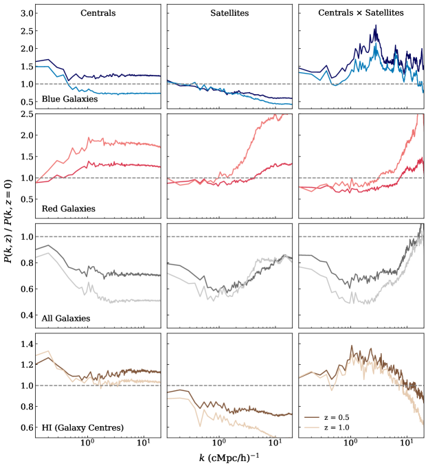
Figure 11: Redshift evolution of the blue (first row), red (second), all-galaxy (third), and ${\rm H}$ i (last) auto power spectra split into contributions from centrals ($P_{c\times c}$, left), satellites ($P_{s\times s}$, centre), and their cross-correlation ($P_{c\times s}$, right) according to equation 9. Power spectra at $z=1$ (lighter colours) and $z=0.5$ (darker) are normalised by the corresponding $z=0$ power spectra, such that power spectra monotonically increasing from $z=1$ to $z=0$ approach unity from below and those decreasing from above. We employ the Galaxy Centres ${\rm H}$ i models to more clearly distinguish centrals and satellites in the ${\rm H}$ i distribution, and display only the mean of the resulting power spectra for visibility. The blue galaxies and ${\rm H}$ i power spectra lose a substantial contribution from the $P_{c\times s}$ term between $z=0.5$ and $z=0$, with a smaller loss from $P_{c\times c}$. Red galaxies, on the other hand, lose considerable power on small scales from all terms, especially from $P_{s\times s}$. These trends provide deeper insight into the processes responsible for the unexpected redshift evolutions found in Section 3 (see text).

We have characterized the clustering of ${\rm H}$ i as a function of colour, redshift, $M_{\star}$, and $M_{\mathrm{HI}}$, often alluding to the influence of baryonic processes on these relationships. In particular, we attributed much of the inverse redshift evolution of the power spectra from Section 3.3 to baryonic processes, but did not determine the precise mechanisms responsible and scales at which they take place. Previous studies of the redshift evolution of red galaxy clustering have proposed mergers, disruption, galaxy quenching and some combination thereof as possible mechanisms that suppress structure growth in galaxies (Zehavi et al., 2005a; White et al., 2007; Guo et al., 2013). In our analysis, we have introduced colour transitions and gas loss as alternative suppression mechanisms. We attempt to disentangle these processes in the redshift evolution of the power spectra in Section 3.3 by considering the clustering of smaller galactic subpopulations. We first decompose the power spectra into contributions from centrals and satellites. Next, we describe how colour transitions and gas loss manifest in each component. We finish by briefly describing whether the redshift evolution of these terms can be explained with other processes, such as mergers and galaxy interactions.

We separate the blue, red, all-galaxy, and ${\rm H}$ i auto powers into contributions from centrals and satellites to provide insight into the processes that govern their time evolution, shown in Fig. 11. We use Galaxy Centres for the ${\rm H}$ i distribution in order to more clearly distinguish between centrals and satellites, but this should have little effect on our conclusions here (Section 3.1). Okumura et al. (2015) provide the following framework for separating the galaxy auto power spectra into central and satellite components,

$$P(k)=(1-f_{s})^{2}P_{c\times c}(k)+2f_{s}(1-f_{s})P_{c\times s}(k)+f_{s}^{2}P_{s\times s}(k)\,,$$ (9)

where the contributions from centrals (c) and satellites (s) are denoted in subscripts and $f_{s}$ represents the satellite fraction. Each term from equation 9 contributes differently at various spatial scales, depending on the shape of the term itself and the corresponding $f_{s}$ coefficients (see figure 1 in Okumura et al., 2015). By definition, there is only one central per halo, so $P_{c\times c}$ is dominated by shot noise in the one-halo regime. The red galaxy auto power spectrum, however, is dominated by $P_{s\times s}$ on all scales because of the high satellite fraction for red galaxies ($f_{s}\sim 0.8$ in TNG100). In contrast, the small satellite fraction for blue galaxies ($f_{s}\sim 0.3$) significantly down-weights $P_{s\times s}$. We now study the evolution of the terms from equation 9 in Fig. 11.

Every term from the all-galaxies power spectra increases with time (third row), retaining the structure growth seen in the full power spectrum from Section 3.3, whereas the evolution in other tracers is significantly more nuanced. Each component of the blue galaxies (top row) and ${\rm H}$ i (bottom row) increases slightly between $z=1$ and $z=0.5$ in Fig. 11, before both of the central-dependent terms ($P_{c\times c}$ and $P_{c\times s}$) decrease between $z=0.5$ and $z=0$. Red galaxies (second row), on the other hand, cluster less with time in every term on small scales. This effect is particularly strong in the $P_{s\times s}$ term, where the clustering of satellites falls by a factor of 2.5 from $z=1$ to $z=0$.

We now analyse how colour transitions affect the previously described evolutions from Fig. 11. As described in Section 3.3, colour transitions suppress clustering by adding relatively weakly clustered galaxies to the red population and removing strongly clustered galaxies from blue. The impact of colour transitions is most visible in the suppression of the clustering of blue centrals (top right panel of Fig. 11), suggesting transitioning blue centrals are primarily responsible for the decreasing power spectrum between $z=0.5$ and $z=0$. The suppression in $P_{c\times c}$ (left) is strongest at largest scales, where transitioning blue centrals dominate because they tend to occupy the most massive blue-hosting haloes. However, in the case of $P_{c\times s}$ (right), the massive haloes hosting transitioning centrals contribute substantially more to smaller scales because they possess the highest satellite fractions amongst blue-hosting haloes. Consequently, when all the central-satellite pairs from that halo are removed after their central transitions, $P_{c\times s}$ decreases significantly at the boundary between the one-halo and two-halo regimes ($k\sim 2$ h cMpc^-1). Previous studies of galaxy quenching in IllustrisTNG indicate that AGN feedback is largely responsible for the colour transitions in these centrals, particularly when their mass reaches the sharp transition at $M_{\star}\geq 10^{10.5}M_{\odot}$ (Zinger et al., 2020; Donnari et al., 2021a). The last term, $P_{s\times s}$ (middle), still increases with time, indicating that colour transitions are less effective at removing power from blue satellites.

In the case of the red population, transitioning galaxies influence their clustering on small scales rather than large scales. As depicted in the middle row of Fig. 11, $P_{c\times c}$ (left) is suppressed moderately at the smallest scales of the two-halo regime ($k\sim 1$ h cMpc^-1), while $P_{s\times s}$ and $P_{c\times s}$ decrease drastically almost entirely within the one-halo regime. Transitioning galaxies inhabit the smallest and youngest red-hosting haloes, which contribute most to small-scale red galaxy clustering, as large scales are dominated by the largest haloes. This is particularly true for the clustering of satellites, as new red-hosting haloes have smaller satellite fractions and satellite quenched fractions (Donnari et al., 2021b).

The other baryonic process we examine is gas loss, which only directly impacts the clustering of ${\rm H}$ i but not of galaxies. The evolution of ${\rm H}$ i auto power spectrum components (bottom row) echo the corresponding blue terms (top row), although with a few additional subtleties. When a galaxy transitions from blue to red, it is completely removed from the blue distribution. The associated gas loss, however, simply down-weights previous contributions of that galaxy to the ${\rm H}$ i auto power spectrum. This mitigates the inverse evolution of the $P_{c\times c}$ (left) and $P_{c\times s}$ (right) terms at $z=0.5$ to $z=0$ as compared to blue galaxies. Similarly to the effect of colour transitions on blue galaxies, we attribute the abating ${\rm H}$ i power spectrum primarily to the rapid gas loss in and around centrals. The allocation of ${\rm H}$ i between centrals and satellites in massive haloes further supports this conclusion. VN18 find that satellites contain most of the ${\rm H}$ i in $M_{h}\gtrsim 10^{13}M_{\odot}$ haloes at $z\leq 1$ (see their figure 7). The ${\rm H}$ i profiles of these haloes provide further evidence for gas loss in and around centrals. The profiles of $M_{h}\sim 10^{13}M_{\odot}$ haloes contain $\sim 10$ kpc / h “holes” around their centres which steadily deepen and broaden with time, a characteristic also found in massive galaxies from other simulations (Bahé et al., 2016; Stevens et al., 2023). At $z=0$, $M_{h}\sim 10^{12}M_{\odot}$ haloes also develop similar features in their profiles (see figure 5 from VN18), showing an increased prevalence of this characteristic at later times even at lower-mass haloes. This phenomenon supports our conclusion that gas loss near the centres of previously gas-rich haloes suppresses the growth of the ${\rm H}$ i auto power spectrum.

Colour transitions and gas loss do not comprise an exhaustive list of mechanisms that can suppress power spectra. Mergers and disruptions, for example, can also impede the rate of clustering growth in the one-halo regime by reducing the number density of satellites (Bell et al., 2004; Skelton et al., 2009; Guo et al., 2013). However, mergers are unlikely to elicit the decrease in blue galaxy clustering, as blue galaxies merge at a relatively slow rate (Lin et al., 2008; Darg et al., 2010). Red galaxies appear to follow this description in the $P_{s\times s}$ and $P_{c\times s}$ terms, which decrease significantly at small scales. However, the all-galaxy $P_{s\times s}$ term increases with time at $k\sim 5$ h cMpc^-1 by a factor of $\sim 1.5$, despite red galaxies decreasing by a factor of $\sim 2$ at the same scale. Mergers should affect both the red and all-galaxy $P_{s\times s}$ terms (Watson et al., 2011), particularly at $z=0$ where red galaxies comprise $\sim 70\%$ of the mass in satellites. However, we note that our reasoning throughout this section neglects the impact of galaxies crossing our imposed resolution limit and centrals becoming satellites between redshifts. Properly disentangling the contributions of various baryonic processes requires sophisticated modelling (Guo et al., 2013), which we leave for future work.

In summary, we find evidence that previously neglected baryonic processes, namely colour transitions and gas loss, significantly influence the clustering of blue and red galaxies and ${\rm H}$ i at $z\leq 1$ such that the power spectra for these populations decrease with time. We identify the signatures of colour transitions and gas loss in the evolution of the terms from equation 9 in Fig. 11. These processes in (previously) gas-rich and star-forming haloes appear particularly effective at suppressing the clustering of each population.

5 Conclusions

We have presented the first systematic investigation of the cross-power spectra of ${\rm H}$ i and galaxies split into colour subpopulations in IllustrisTNG and studied how their clustering changes with time and various galaxy properties. We find the following:

1. The clustering of simulated ${\rm H}$ i distributions exhibits only a weak dependence on the model for the transition between atomic and molecular hydrogen.

2. The ${\rm H}$ i-red galaxy cross-power spectrum (${\rm H}$ i $\times$ Red) is greater than ${\rm H}$ i-blue (${\rm H}$ i $\times$ Blue) at large scales due to red galaxies’ inherent clustering strength and larger bias with respect to matter. However, processes such as AGN feedback and ram-pressure stripping suppress ${\rm H}$ i abundance in the massive haloes that red galaxies typically occupy, weakening ${\rm H}$ i $\times$ Red on small scales and creating an intersection between ${\rm H}$ i $\times$ Red and ${\rm H}$ i $\times$ Blue at $\approx 3$ Mpc at $z=0$.

3. In redshift space, the suppression of power due to the fingers-of-God effect manifests more strongly in red galaxies than blue galaxies, introducing a secondary colour-dependency and pushing the intersection of ${\rm H}$ i $\times$ Red and ${\rm H}$ i $\times$ Blue to $\approx 10$ Mpc at $z=0$.

4. The ${\rm H}$ i, red, and blue galaxy auto power spectra and their cross-power spectra decrease with cosmic time, contrary to the clustering of matter and the galaxy population as a whole. Colour transitions in galaxies and ${\rm H}$ i consumption contribute to this inverse evolution. These baryonic processes may need to be taken into account in models of the large-scale distribution of these populations at $z<1$.

5. ${\rm H}$ i $\times$ Blue increases as a function of $M_{\star}$. ${\rm H}$ i $\times$ Red also reflects this trend, until $M_{\star}\approx 10^{10}M_{\odot}$ where the clustering is the weakest amongst the stellar mass bins examined. Red galaxies below this threshold are typically satellites that occupy massive haloes more frequently than the red centrals in larger $M_{\star}$ bins.

6. Satellites correlate more strongly with ${\rm H}$ i with increasing $M_{\star}$, whereas centrals correlate less strongly. These trends hold regardless of galaxy colour.

7. The ${\rm H}$ i clustering increases as a function of $M_{\mathrm{HI}}$, and galaxies with $M_{\mathrm{HI}}\geq 10^{8}M_{\odot}$ dominate the total ${\rm H}$ i auto power spectrum. We show that ${\rm H}$ i auto power spectra should be unbiased as long as the survey captures galaxies with $M_{\mathrm{HI}}\geq 10^{8}M_{\odot}$.

These conclusions are important for future 21cm surveys, where detections occur in the first phases as cross-correlations. These results contribute to the theoretical formalism needed to extract cosmological constraints from upcoming 21cm surveys and better understand the ${\rm H}$ i-galaxy-halo connection. We have established that the baryonic processes associated with quenching can have large-scale imprints on the clustering of ${\rm H}$ i, blue, and red galaxies. Models of the bias with respect to matter of these populations rely on simplistic assumptions about their growth and scale-dependence, which may skew the interpretation of the data from 21cm surveys, as we will explore in future work (Osinga et al., in prep.).

One caveat to our results is that they were derived from a single suite of simulations, IllustrisTNG. Repeating our analysis with other simulations could illuminate whether these relationships are sensitive to the simulation’s model for galaxy formation and evolution. For example, it is unclear whether or not the cosmic abundance of ${\rm H}$ i ($\Omega_{\rm{HI}}$) in IllustrisTNG is consistent with observations in the redshifts studied here (Villaescusa-Navarro et al., 2018; Diemer et al., 2019). Furthermore, mock-observing IllustrisTNG would allow for more faithful comparisons with observations and further our understanding of how observational effects manifest in the clustering relationships examined here. For example, Donnari et al. (2021b) showed that quenched fractions are quite sensitive to observational effects.

Appendix A Sensitivity to colour cut

Figure 12: The sensitivity of ${\rm H}$ i $\times$ Blue (top) and ${\rm H}$ i $\times$ Red (bottom) to the colour cut and dust (gray) at $z=0$. The cross-power spectra calculated with colour cuts at two extremes $g\!$ - $\!r$ = 0.55 (dark) and $g\!$ - $\!r$ = 0.65 (light) are shown as a ratio over the fiducial $g\!$ - $\!r$ = 0.60 cut. We apply $g\!$ - $\!r$ = 0.60 for the dust prescription from Nelson et al. (2018). We plot the centre of the contours encompassing ${\rm H}$ i models from the alternate $g\!$ - $\!r$ cuts for visibility, but they have similar widths to the dust contour. Particularly in the two-halo regime, power spectra are insensitive to the colour threshold.

Throughout the paper, we have assumed a single definition of the colour cut to separate blue and red galaxies. Here, we analyse the sensitivity of the cross-power spectra to alternate colour cuts and the inclusion of dust (Nelson et al., 2018). ${\rm H}$ i $\times$ Red and ${\rm H}$ i $\times$ Blue using these alternative colour definitions at $z=0$ are displayed as a ratio over the fiducial colour cut in Fig. 12. The colour cut can change the resulting clustering by a factor of $\sim 1.2$ for both blue and red galaxies on small scales, whereas on large scales the changes are negligible. At earlier redshifts, the smaller red population grows more sensitive to colour cut, but the effect is still a factor of $\sim 1.5$ overall.

Dust corrections redden blue galaxies more than red ones, essentially squeezing the galaxy distribution along the $g\!$ - $\!r$ axis. Similar to the colour cuts, modelling dust effects in the photometry from IllustrisTNG has a negligible impact on the resulting clustering on large scales. On small scales, dust effects are stronger, with ${\rm H}$ i $\times$ Blue falling below the fiducial definition by a factor of $\sim 0.6$ and ${\rm H}$ i $\times$ Red increasing by a factor of $\sim 1.2$. We attribute the colour cut insensitivity to the relatively low occupation in the green valley. As long as the colour cut reasonably splits the colour modes, the clustering is comparable.

Appendix B Convergence Tests

In this section, we ascertain the convergence of our results. We first test convergence of ${\rm H}$ i $\times$ Red and ${\rm H}$ i $\times$ Blue with mass resolution in Fig. 13. In the overlapping $k$ range TNG100-2 and TNG300-1 agree for both colours, which is reassuring since they have roughly the same mass resolution. Since a non-negligible proportion of the cosmic ${\rm H}$ i belongs to galaxies below the TNG100-2 mass resolution threshold, the galaxies from TNG100-1 correlate more strongly with ${\rm H}$ i than the other simulations. ${\rm H}$ i $\times$ Red from lower resolution simulations can fall a factor of $\sim 0.5$ below the TNG100-1 result, whereas ${\rm H}$ i $\times$ Blue remains at $\sim 0.8$ throughout different scale regimes. The relatively small magnitude of the effect reassures us that they are not sensitive to mass resolution—the normalisations of the cross-power spectra are slightly resolution-dependent, but the trends are not.

We also test how our results change with increasing grid resolution. We binned mass distributions in $800^{3}$, $1000^{3}$, and $1200^{3}$ grids and found no visible difference between them. This comparison is provided in the online figures.

Since we arbitrarily picked a line of sight to project the velocities of matter on, we also projected our redshift-space power spectra along different axes. The cross-power spectra calculated from distributions displaced along different axes should not necessarily match, as matter will collapse faster along one axis than the others (Zel’dovich, 1970). Our results on large scales can vary by a factor of $\sim 15\%$ due to the axis chosen. This comparison is also provided in the online figures.

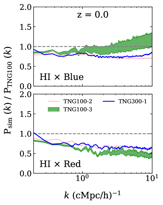
Figure 13: Convergence of ${\rm H}$ i $\times$ Blue (top) and ${\rm H}$ i $\times$ Red (bottom) with mass resolution at $z=0$, shown as a ratio over the fiducial TNG100 simulation resolution. The lower resolution versions of TNG100, TNG100-2 (pink) and TNG100-3 (green) are displayed in fainter colours. For visibility, we only plot the contour delineating ${\rm H}$ i models for TNG100-3, but the widths are otherwise similar. The effect of mass resolution is overall small, but does not clearly converge to the fiducial result.

References

- Abadi et al. (1999) Abadi M. G., Moore B., Bower R. G., 1999, MNRAS, 308, 947
- Akins et al. (2022) Akins H. B., Narayanan D., Whitaker K. E., Davé R., Lower S., Bezanson R., Feldmann R., Kriek M., 2022, ApJ, 929, 94
- Anderson et al. (2018) Anderson C. J., et al., 2018, MNRAS, 476, 3382
- Ayromlou et al. (2023) Ayromlou M., Kauffmann G., Anand A., White S. D. M., 2023, MNRAS, 519, 1913
- Bahé et al. (2016) Bahé Y. M., et al., 2016, MNRAS, 456, 1115
- Balogh et al. (2004) Balogh M. L., Baldry I. K., Nichol R., Miller C., Bower R., Glazebrook K., 2004, ApJ, 615, L101
- Bandura et al. (2014) Bandura K., et al., 2014, in Stepp L. M., Gilmozzi R., Hall H. J., eds, Society of Photo-Optical Instrumentation Engineers (SPIE) Conference Series Vol. 9145, Ground-based and Airborne Telescopes V. p. 914522 (arXiv:1406.2288), doi:10.1117/12.2054950
- Basilakos et al. (2007) Basilakos S., Plionis M., Kovač K., Voglis N., 2007, MNRAS, 378, 301
- Bell et al. (2004) Bell E. F., et al., 2004, ApJ, 608, 752
- Berlind & Weinberg (2002) Berlind A. A., Weinberg D. H., 2002, ApJ, 575, 587
- Beutler et al. (2013) Beutler F., et al., 2013, MNRAS, 429, 3604
- Bigiel et al. (2008) Bigiel F., Leroy A., Walter F., Brinks E., de Blok W. J. G., Madore B., Thornley M. D., 2008, AJ, 136, 2846
- Brown et al. (2021) Brown T., et al., 2021, ApJS, 257, 21
- Chang et al. (2010) Chang T.-C., Pen U.-L., Bandura K., Peterson J. B., 2010, Nature, 466, 463
- Coil et al. (2017) Coil A. L., Mendez A. J., Eisenstein D. J., Moustakas J., 2017, The Astrophysical Journal, 838, 87
- Colless et al. (2001) Colless M., et al., 2001, MNRAS, 328, 1039
- Collette et al. (2021) Collette A., et al., 2021, h5py/h5py: 3.5.0, Zenodo, doi:10.5281/zenodo.5585380
- Cosmic Visions 21 cm Collaboration et al. (2018) Cosmic Visions 21 cm Collaboration et al., 2018, arXiv e-prints, p. arXiv:1810.09572
- Cunnington et al. (2023) Cunnington S., et al., 2023, MNRAS, 518, 6262
- Daddi et al. (2007) Daddi E., et al., 2007, ApJ, 670, 156
- Darg et al. (2010) Darg D. W., et al., 2010, MNRAS, 401, 1552
- Davé et al. (2017) Davé R., Rafieferantsoa M. H., Thompson R. J., 2017, MNRAS, 471, 1671
- Davé et al. (2019) Davé R., Anglés-Alcázar D., Narayanan D., Li Q., Rafieferantsoa M. H., Appleby S., 2019, MNRAS, 486, 2827
- Davé et al. (2020) Davé R., Crain R. A., Stevens A. R. H., Narayanan D., Saintonge A., Catinella B., Cortese L., 2020, MNRAS, 497, 146
- Davis et al. (1985) Davis M., Efstathiou G., Frenk C. S., White S. D. M., 1985, ApJ, 292, 371
- Dewdney et al. (2009) Dewdney P. E., Hall P. J., Schilizzi R. T., Lazio T. J. L. W., 2009, IEEE Proceedings, 97, 1482
- Diemer (2018) Diemer B., 2018, ApJS, 239, 35
- Diemer et al. (2018) Diemer B., et al., 2018, ApJS, 238, 33
- Diemer et al. (2019) Diemer B., et al., 2019, MNRAS, 487, 1529
- Dodelson & Schmidt (2020) Dodelson S., Schmidt F., 2020, Modern Cosmology, doi:10.1016/C2017-0-01943-2.
- Donnari et al. (2019) Donnari M., et al., 2019, MNRAS, 485, 4817
- Donnari et al. (2021a) Donnari M., et al., 2021a, MNRAS, 500, 4004
- Donnari et al. (2021b) Donnari M., Pillepich A., Nelson D., Marinacci F., Vogelsberger M., Hernquist L., 2021b, MNRAS, 506, 4760
- Draine (2011) Draine B. T., 2011, Physics of the Interstellar and Intergalactic Medium
- Eisenstein et al. (2005) Eisenstein D. J., et al., 2005, ApJ, 633, 560
- Faucher-Giguère et al. (2009) Faucher-Giguère C.-A., Lidz A., Zaldarriaga M., Hernquist L., 2009, ApJ, 703, 1416
- Ferland et al. (2017) Ferland G. J., et al., 2017, Rev. Mex. Astron. Astrofis., 53, 385
- Fry (1996) Fry J. N., 1996, ApJ, 461, L65
- Gao et al. (2005) Gao L., Springel V., White S. D. M., 2005, MNRAS, 363, L66
- Gebek et al. (2023) Gebek A., et al., 2023, MNRAS, 521, 5645
- Giovanelli & Haynes (1985) Giovanelli R., Haynes M. P., 1985, ApJ, 292, 404
- Giovanelli et al. (2005) Giovanelli R., et al., 2005, AJ, 130, 2598
- Gnedin & Draine (2014) Gnedin N. Y., Draine B. T., 2014, ApJ, 795, 37
- Gnedin & Kravtsov (2011) Gnedin N. Y., Kravtsov A. V., 2011, ApJ, 728, 88
- Gomersall (2021) Gomersall H., 2021, Astrophysics Source Code Library, pp ascl–2109
- Gómez et al. (2003) Gómez P. L., et al., 2003, ApJ, 584, 210
- Gunn & Gott (1972) Gunn J. E., Gott J. Richard I., 1972, ApJ, 176, 1
- Guo et al. (2011) Guo Q., et al., 2011, MNRAS, 413, 101
- Guo et al. (2013) Guo H., et al., 2013, ApJ, 767, 122
- Guo et al. (2014) Guo H., et al., 2014, MNRAS, 441, 2398
- Guo et al. (2017) Guo H., Li C., Zheng Z., Mo H. J., Jing Y. P., Zu Y., Lim S. H., Xu H., 2017, ApJ, 846, 61
- Hadzhiyska et al. (2020) Hadzhiyska B., Bose S., Eisenstein D., Hernquist L., Spergel D. N., 2020, MNRAS, 493, 5506
- Harris et al. (2020) Harris C. R., et al., 2020, Nature, 585, 357
- Haynes et al. (2011) Haynes M. P., et al., 2011, AJ, 142, 170
- Hearin et al. (2016) Hearin A. P., Behroozi P. S., van den Bosch F. C., 2016, Monthly Notices of the Royal Astronomical Society, 461, 2135
- Henriques et al. (2017) Henriques B. M. B., White S. D. M., Thomas P. A., Angulo R. E., Guo Q., Lemson G., Wang W., 2017, MNRAS, 469, 2626
- Hunter (2007) Hunter J. D., 2007, Computing in Science and Engineering, 9, 90
- Jackson (1972) Jackson J. C., 1972, MNRAS, 156, 1P
- Jenkins et al. (1998) Jenkins A., et al., 1998, ApJ, 499, 20
- Jiang et al. (2023) Jiang Y., et al., 2023, Cross-Correlation Forecast of CSST Spectroscopic Galaxy and MeerKAT Neutral Hydrogen Intensity Mapping Surveys (arXiv:2301.02540)
- Jiménez-Donaire et al. (2023) Jiménez-Donaire M. J., et al., 2023, A&A, 671, A3
- Juszkiewicz et al. (2000) Juszkiewicz R., Ferreira P. G., Feldman H. A., Jaffe A. H., Davis M., 2000, Science, 287, 109
- Kaiser (1987) Kaiser N., 1987, MNRAS, 227, 1
- Kauffmann et al. (2013) Kauffmann G., Li C., Zhang W., Weinmann S., 2013, MNRAS, 430, 1447
- Kennicutt (1998) Kennicutt Robert C. J., 1998, ApJ, 498, 541
- Kravtsov et al. (2004) Kravtsov A. V., Berlind A. A., Wechsler R. H., Klypin A. A., Gottlöber S., Allgood B., Primack J. R., 2004, ApJ, 609, 35
- Krumholz (2013) Krumholz M. R., 2013, MNRAS, 436, 2747
- Krumholz et al. (2008) Krumholz M. R., McKee C. F., Tumlinson J., 2008, ApJ, 689, 865
- Krumholz et al. (2009) Krumholz M. R., McKee C. F., Tumlinson J., 2009, ApJ, 693, 216
- Larson et al. (1980) Larson R. B., Tinsley B. M., Caldwell C. N., 1980, ApJ, 237, 692
- Leo et al. (2019) Leo M., Arnold C., Li B., 2019, Physical Review D, 100
- Leroy et al. (2008) Leroy A. K., Walter F., Brinks E., Bigiel F., de Blok W. J. G., Madore B., Thornley M. D., 2008, AJ, 136, 2782
- Li et al. (2006) Li C., Jing Y., Kauffmann G., Börner G., White S. D., Cheng F., 2006, Monthly Notices of the Royal Astronomical Society, 368, 37
- Li et al. (2012) Li C., Kauffmann G., Fu J., Wang J., Catinella B., Fabello S., Schiminovich D., Zhang W., 2012, MNRAS, 424, 1471
- Li et al. (2022) Li X., Li C., Mo H. J., Xiao T., Wang J., 2022, arXiv e-prints, p. arXiv:2209.07691
- Lin et al. (2008) Lin L., et al., 2008, The Astrophysical Journal, 681, 232
- Madau et al. (1996) Madau P., Ferguson H. C., Dickinson M. E., Giavalisco M., Steidel C. C., Fruchter A., 1996, MNRAS, 283, 1388
- Marasco et al. (2016) Marasco A., Crain R. A., Schaye J., Bahé Y. M., van der Hulst T., Theuns T., Bower R. G., 2016, MNRAS, 461, 2630
- Marinacci et al. (2018) Marinacci F., et al., 2018, MNRAS, 480, 5113
- Masui et al. (2013) Masui K. W., et al., 2013, ApJ, 763, L20
- Meyer et al. (2007) Meyer M. J., Zwaan M. A., Webster R. L., Brown M. J. I., Staveley-Smith L., 2007, ApJ, 654, 702
- Moore et al. (1996) Moore B., Katz N., Lake G., Dressler A., Oemler A., 1996, Nature, 379, 613
- Moore et al. (1998) Moore B., Lake G., Katz N., 1998, ApJ, 495, 139
- Naiman et al. (2018) Naiman J. P., et al., 2018, MNRAS, 477, 1206
- Nelson et al. (2018) Nelson D., et al., 2018, MNRAS, 475, 624
- Newburgh et al. (2016) Newburgh L. B., et al., 2016, in Hall H. J., Gilmozzi R., Marshall H. K., eds, Society of Photo-Optical Instrumentation Engineers (SPIE) Conference Series Vol. 9906, Ground-based and Airborne Telescopes VI. p. 99065X (arXiv:1607.02059), doi:10.1117/12.2234286
- Noeske et al. (2007) Noeske K. G., et al., 2007, ApJ, 660, L43
- Okumura et al. (2015) Okumura T., Hand N., Seljak U. c. v., Vlah Z., Desjacques V., 2015, Phys. Rev. D, 92, 103516
- Papastergis et al. (2013) Papastergis E., Giovanelli R., Haynes M. P., Rodríguez-Puebla A., Jones M. G., 2013, ApJ, 776, 43
- Paul et al. (2023) Paul S., Santos M. G., Chen Z., Wolz L., 2023, arXiv e-prints, p. arXiv:2301.11943
- Peacock & Smith (2000) Peacock J. A., Smith R. E., 2000, MNRAS, 318, 1144
- Pillepich et al. (2018a) Pillepich A., et al., 2018a, MNRAS, 473, 4077
- Pillepich et al. (2018b) Pillepich A., et al., 2018b, MNRAS, 475, 648
- Planck Collaboration et al. (2016) Planck Collaboration et al., 2016, A&A, 594, A13
- Qin et al. (2022) Qin F., Howlett C., Stevens A. R. H., Parkinson D., 2022, arXiv e-prints, p. arXiv:2208.11454
- Rahmati et al. (2013) Rahmati A., Schaye J., Pawlik A. H., Raičević M., 2013, MNRAS, 431, 2261
- Reddick et al. (2014) Reddick R. M., Tinker J. L., Wechsler R. H., Lu Y., 2014, ApJ, 783, 118
- Schmidt (1959) Schmidt M., 1959, ApJ, 129, 243
- Skelton et al. (2009) Skelton R. E., Bell E. F., Somerville R. S., 2009, ApJ, 699, L9
- Skibba et al. (2014) Skibba R. A., et al., 2014, ApJ, 784, 128
- Skibba et al. (2015) Skibba R. A., et al., 2015, ApJ, 807, 152
- Solanes et al. (2002) Solanes J. M., Sanchis T., Salvador-Solé E., Giovanelli R., Haynes M. P., 2002, AJ, 124, 2440
- Springel (2010) Springel V., 2010, ARA&A, 48, 391
- Springel & Hernquist (2003) Springel V., Hernquist L., 2003, MNRAS, 339, 289
- Springel et al. (2001) Springel V., White S. D. M., Tormen G., Kauffmann G., 2001, MNRAS, 328, 726
- Springel et al. (2018) Springel V., et al., 2018, MNRAS, 475, 676
- Staveley-Smith et al. (1996) Staveley-Smith L., et al., 1996, Publ. Astron. Soc. Australia, 13, 243
- Sternberg et al. (2014) Sternberg A., Le Petit F., Roueff E., Le Bourlot J., 2014, ApJ, 790, 10
- Stevens et al. (2019) Stevens A. R. H., et al., 2019, MNRAS, 483, 5334
- Stevens et al. (2023) Stevens A. R. H., et al., 2023, arXiv e-prints, p. arXiv:2310.08023
- Stoughton et al. (2002) Stoughton C., et al., 2002, AJ, 123, 485
- Tinker et al. (2005) Tinker J. L., Weinberg D. H., Zheng Z., Zehavi I., 2005, ApJ, 631, 41
- Tinsley (1980) Tinsley B. M., 1980, Fundamentals Cosmic Phys., 5, 287
- Villaescusa-Navarro (2018) Villaescusa-Navarro F., 2018, Pylians: Python libraries for the analysis of numerical simulations, Astrophysics Source Code Library, record ascl:1811.008 (ascl:1811.008)