The intelligent agent model – a fully two-dimensional microscopic traffic flow model

Abstract

Recently, a fully two-dimensional microscopic traffic flow model for lane-free vehicular traffic flow has been proposed [Physica A, 509, pp. 1-11 (2018)]. In this contribution, we generalize this model to describe any kind of human-driven directed flow including lane-based vehicular flow, lane-free mixed traffic, bicycle traffic, and pedestrian flow. The proposed intelligent-agent model (IAM) has the same philosophy as the well-known social-force model (SFM) for pedestrians but the interaction and boundary forces are based on car-following models making this model suitable for higher speeds. Depending on the underlying car-following model, the IAM includes anticipation, response to relative velocities, and accident-free driving. When adding a suitable floor field, the IAM reverts to an integrated car-following and lane-changing model with continuous lane changes. We simulate this model in several lane-based and lane-free environments in various geometries with and without obstacles. We observe that the model produces accident-free traffic flow reproducing the observed self-organisation phenomena.

1 Introduction

Microscopic traffic flow models traditionally describe the flow in a continuous longitudinal and discrete lateral dimension in form of car-following and lane-changing models TreiberKesting-Book . In traffic flow simulators such as VISSIM VISSIM or SUMO SUMO2011 , both components are integrated into a common model. These traditional models, however, are not able to describe disordered lane-free traffic flow consisting of a wide variety of vehicle sizes and properties which is typically observed in developing countries. This type of flow is characterized by a continuous lateral degree of freedom requiring a fully two-dimensional model. Generalizing lane-changing models with incentives in terms of acceleration differences Hidas-02 ; MOBIL-TRR07 , a first fully two-dimensional model for mixed vehicular flow with lateral forces proportional to longitudinal acceleration shears has been proposed, the mixed-traffic model (MTM) Kanagaraj2018self .

However, this model only reacts to vehicles in the front and also has a rather complicated formulation of the lateral forces making it hard to calibrate. In contrast, the social-force model (SFM) for pedestrians by Helbing and Molnár SFM has a clean formulation. There, the acceleration of each pedestrian is given by the superposition of the free-flow social force, the interaction forces exerted by the pedestrians nearby, and the repulsive forces of the boundaries. However, the SFM cannot be applied to vehicles, cyclists or other self-driven agents with a higher speed since it does not contain the kinematic constraints of a limited acceleration, is not crash free, and does not revert to a plausible car-following model in case of single-file traffic. This is also the case for other pedestrian flow models chen2018social .

On the other hand, there exist several car-following models for mixed traffic which, however, only modify the model parameters depending on the lateral offset or the kind of leaders and followers asaithambi2018study ; madhu2023vehicle while not incorporating any lateral dynamics itself.

In this contribution, we propose the intelligent-agent model (IAM) which is an integration of the (simplified) MTM for vehicular traffic and the SFM for pedestrians. As the MTM, it is based on a car-following model to which it reverts for single-file traffic and from which it inherits all the properties for a safe high-speed motion. It also contains aspects of the social-force model such as the superposition of the social forces of all active agents nearby (including the back) with a directional weighting. Optionally, we also introduce floor fields to transform the originally lane-free formulation to a lane-based environment. In this case, the IAM reverts to an integrated car-following and lane-changing model with continuous lane changes.

In Sect. 2, we formulate our proposed model IAM. In Section 3, we simulate it with the underlying Intelligent-Driver-Model Opus ; traffic-simulation in several lane-based and lane-free environments with mixed vehicular-bicycle traffic and pure bicycle traffic. We conclude with a discussion in Sect. 4.

2 Model specification

As the SFM, the proposed IAM is based on social forces which can be subdivided into the self-driving force to reach the destination with a desired speed, the interaction forces with other moving and standing objects, and boundary forces to keep the agents in the driveable or walkeable area,

$$\frac{{\rm d}\vec{v}_{i}}{{\rm d}t}=\vec{f}^{\rm self}_{i}(\vec{v}_{i})+\sum_{j}\vec{f}^{\rm int}_{ij}(\vec{r}_{i},\vec{v}_{i},\vec{r}_{j},\vec{v}_{j})+\sum_{b}\vec{f}_{ib}.$$ (1)

Unlike the SFM, the IAM is dedicated to directed flows where a local axis of the road or pathway can be defined. Furthermore, the IAM is anisotropic with a distinctively different dynamics for the longitudinal direction (parallel to the axis) and the lateral one. We denote the components of the longitudinal and lateral position vector with $\vec{x}=(x,y)^{\prime}$, and decompose the velocity and force vectors by $\vec{v}=(v,w)^{\prime}$ and $\vec{f}=(f,g)^{\prime}$, respectively. Setting the agent’s mass $m=1$, the forces also denote the accelerations, $\vec{f}=(\dot{v},\dot{w})^{\prime}$.

2.1 Self-driving forces

The longitudinal part of the self-driving force is derived from the underlying car-following (CF) which we characterize by the general acceleration function $\dot{v}\equiv\frac{{\rm d}v}{{\rm d}t}=f^{\rm CF}(s,v,v_{l})$ depending on the (bumper-to-bumper) gap $s$ to the leader, the subject’s speed $v$, and the leading speed $v_{l}$. We derive the self-driving force by decomposing this model as

$$f^{\rm CF}(s,v,v_{l})=f^{\rm self}(v)+f^{\rm CF,int}(s,v,v_{l}),\quad f^{\rm self}(v)=f^{\rm CF}(s\to\infty,v,v),$$ (2)

where $f^{\rm CF,int}=f^{\rm CF}-f^{\rm self}$ denotes the CF force in case of a strictly single-file traffic. Notice that the desired speed $v_{0}$ is given in terms of the implicit relation $f_{\rm CF}(s\to\infty,v_{0},v_{0})=0$.

Since we assume situations where the lateral velocity component is of the order of the pedestrian speed, the free-flow velocity relaxation term of the SFM is appropriate resulting in the lateral self-driving force

$$g^{\rm self}(w)=\frac{w_{0}-w}{\tau_{y}},$$ (3)

where the lateral desired speed $w_{0}=v_{0}e_{y}^{\rm dest}$ is nonzero if the unit vector $\vec{e}^{\rm dest}$ to the destination is not parallel to the road axis, for example, when entering or leaving the road or bikeway.

2.2 Interaction forces

According to Eq (1), the interacting force is a superposition of the forces $\vec{f}_{ij}^{\rm int}=\left(f_{ij}^{\rm int},g_{ij}^{\rm int}\right)^{\prime}$ of the nearby agents including standing objects, e.g., the stopping line of a red traffic light which is represented by a very wide and very short virtual vehicle with the outline of the stopping line. In the following, we define the longitudinal and lateral forces exerted by an agent/object $j$ as a function of $\vec{x}_{j}$ and $\vec{v}_{j}$.

Longitudinal interaction forces

We assume that the longitudinal interaction is that of the CF model whenever the follower’s occupancy area laterally encroaches that of the leader. If the lateral speeds are negligible with respect to the longitudinal ones, encroachment is given if the absolute value of the lateral offset $\Delta y=y_{j}-y_{i}$ is less than the average agent/object with $\overline{W}=(W_{i}+W_{j})/2$. If no encroachment is given, i.e., the lateral gap $s_{y}=|\Delta y|-\overline{W}>0$, the longitudinal force decreases exponentially with $s_{y}$ as in the SFM. This results in

$$f_{ij}^{\rm int}(\vec{x}_{i},\vec{x}_{j},\vec{v}_{i},\vec{v}_{j})=\alpha(s_{y})f^{\rm CF}(s_{x},v_{i},v_{j})$$ (4)

where

$$s_{x}=x_{j}-x_{i}-L_{j},\quad s_{y}=|y_{j}-y_{i}|-\overline{W},\quad\alpha(s_{y})=\min\left(1,e^{-|s_{y}|/s_{0y}}\right).$$ (5)

The underlying CF model must be specified in a way that negative gaps $s_{x}$ (i.e., collisions) result in a maximum deceleration (e.g. $9\,\mathrm{m/s^{2}}$). Furthermore, we assume a longitudinal force of zero if $s_{x}<0$ but $s_{y}>0$, i.e., the agent $j$ drives in parallel.

Interactions from followers As in the SFM, we also include “pushing” interactions from the followers ($x_{j}<x_{i}$) which are weakend by the SFM anisotropy factor $\lambda\leq 1$,

$$f_{ij}^{\rm push}=-\lambda f_{ji}^{\rm int}$$ (6)

With $\lambda=1$, we would have a momentum conserving dynamics (“actio=reactio”) but no longer a defined fundamental diagram, i.e., a steady-state macroscopic flow-density relation. Plausible values (of the order of $\lambda=0.1$) increase the flow efficiency without leading to more critical situations.

Total longitudinal interaction Reacting to more than one leader or follower can lead to inconsistent results if there are large size differences between the agents. For example, three cyclists driving in parallel and followed by a truck will not exert on the truck driver the triple social force. Rather, the truck driver reacts to the slowest and/or nearest bicycle, only. Therefore, the total longitudinal interaction force is given by

$$f_{i}^{\rm int}=\min_{j,x_{j}\geq x_{i}}f_{ij}^{\rm int}+\max_{j,x_{j}<x_{i}}f_{ij}^{\rm push}.$$ (7)

Notice that, even in single-file traffic, the selected leader needs not to be the immediate leader but can also be a red traffic light further downstream.

Lateral interaction forces

Generalizing the incentive criterion of the lane-changing model MOBIL, the lateral incentive exerted by agent $j$ is proportional to the shear of the longitudinal force from this agent. Formulating the incentive in terms of an induced desired lateral velocity $w_{0i}$, we have

$$w_{0,ij}\propto\partial f_{ij}^{\rm int}/\partial y_{i}$$ (8)

leading via (4), as in the SFM, to an exponential decrease of the repulsion if there is no lateral overlap. However, if there is an overlap, the longitudinal force does not change with $y_{i}$ and the lateral incentive is zero. To break this tie, we assume that the lateral incentive linearly increases with the lateral offset in the overlapping region. Inserting (8) into (4) and describing the lateral dynamics, as in the SFM, as a relaxation process, we finally obtain

$$g^{\rm int}_{ij}=\frac{w_{0,ij}-w_{i}}{\tau},\quad w_{0,ij}=\sigma f_{\rm CF}^{\rm int}\left\{\begin{array}[]{ll}\Delta y/\overline{W}&\ \ |\Delta y|\leq\overline{W},\\ \text{sign}(\Delta y)e^{-{s_{y}/s_{0y}}}&\ \ \text{otherwise}.\end{array}\right.$$ (9)

Unlike the longitudinal case, we assume no shielding, so the total lateral interaction force is given by the sum of the forces exerted by all surrounding agents with that of the followers reduced by the anisotropy factor $\lambda$.

Table 1: Model parameters of the IAM in addition of the parameters of the underlying CF model

Parameter	Meaning	Typical value
SFM transversal relaxation time	$\tau_{y}$	1 s
Attenuation width	$s_{0y}$	0.3 m
Boundary attenuation width	$s_{B0}$	0.2 m
SFM anisotropy parameter	$\lambda$	0 - 0.2
Lateral sensitivity	$\sigma$	1 s
long. deceleration at the boundary	$\hat{f}_{\rm B}$	$0.2\,\mathrm{m/s^{2}}$
lat. acceleration at the boundary	$\hat{g}_{\rm B}$	$5\,\mathrm{m/s^{2}}$

t]

Figure 1: Force (acceleration) vector field of all forces of Section 2 for two leaders and road boundary for arbitrary positions ($x,y$) of the follower. Notice that leader 2 (to the right) is bigger, further away, and slower

2.3 Boundary forces and floor fields

In principle, a boundary of a driveable area can be modelled by a series of long obstacles. However, an equivalent dedicated approach is more efficient. When driving near the road boundary or even transgressing it partly, there is not only a strong social force towards the road center but also a weak decelerating force in the longitudinal direction:

$$\vec{f}_{\rm B}(s_{y})=\alpha_{\rm B}(s_{y})\left(-\hat{f}_{\rm B}\frac{v}{v_{0}},\ \pm\hat{g}_{\rm B}\right)^{\prime},\ \alpha_{\rm B}(s)=\min\big{(}1,e^{-s/s_{\rm B0}}\big{)},$$ (10)

where $s_{y}$ is the gap between the boundary and the vehicle ($s_{y}<0$ if the boundary is transgressed) and $\hat{f}_{\rm B}$, $\hat{g}_{\rm B}$ and $s_{\rm B0}$ are model parameters (cf Table 2.2).

Finally, to obtain the resulting acceleration vector caused by the boundaries, all forces from the left and right boundary are added up (Fig. 1).

Floor fields For lane-based flow, we add a periodic floor field:

$$g_{\rm lane}(x,y)=-\frac{\partial\Phi}{\partial y},\quad\Phi(x,y)=\pm\Phi_{0}\cos(2\pi y/W_{\rm lane})$$ (11)

where plus applies for an even lane number (a lane separating line is on the directional road axis) and minus for an uneven number. The maximum induced lateral acceleration is given by $2\pi\Phi_{0}/W_{\rm lane}$.

3 Simulation and validation of lane-based and lane-free scenarios

In this section, we simulate the IAM for two different scenarios: Lane based vehicular traffic (Sect. 3.1) and lane-free bicycle traffic (Sect. 3.2). Both simulations are validated by empirical data.

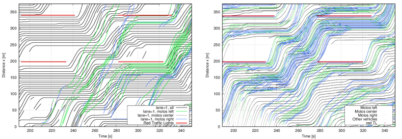
Figure 2: Left: Trajectory data taken from the open-data project pNEUMA pNEUMA . Right: simulation of the IAM with floor fields. In both images, the motorcycles are color-coded whether they drive in the lane (gray) or between the lanes to the left or right (green and blue, respectively).

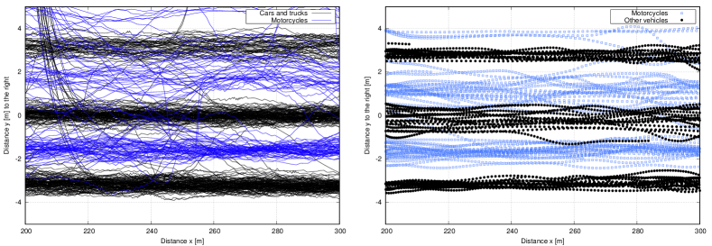
Figure 3: Cross section on the $x$-$y$ plane of the same observed and simulated trajectories as in Fig. 2.

3.1 Lane-based city traffic

The Figs. 2 (left), 3 (left), and 4(left) show naturalistic trajectory data of the second-to-right lane of the Athens arterial Leof. Alexandrias as obtained by the open-data project pNEUMA pNEUMA on Oct 24, 2018. The data show that the motorcyclists generally make use of the space between the lanes (Figs. 3 and  4) to overtake the larger vehicles as seen in the $x$-$t$ cross section of the trajectories at the middle lane and its boundaries (Fig. 2). This leads to a partial segregation of the vehicle types with motorcycles accumulating behind the stopping lines of the red traffic lights (red horizontal lines in Fig. 2) and starting first when the lights turn green.

In the IAM (right plots of the respective figures), this particular situation is modelled by floor fields with a phase shift of $\pi$ between motorcycles and other vehicles. The simulation qualitatively and even semi-quantitatively reproduced all observations such as the longitudinal and lateral vehicle-type segregation, the longitudinal dynamics including the overtaking maneuvers of the motorcyclists (Fig. 2 right), the lane-changing rate (beginning and ending trajectories in Fig. 2, number of crossing trajectories in Fig. 3), and the lateral dynamics during lane changes (Fig. 3).

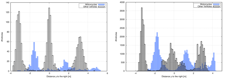
Figure 4: Histogram of the lateral positions of the motorcycles (blue) and the rest of the vehicles (black). Left: real trajectories of the Athens arterial (see Fig. 2); right: simulation of the IAM.

3.2 Lane-free bicycle traffic

To demonstrate the ability of the IAM to simulate lane-free traffic and various observed self-organisation effects wierbos2019capacity , we simulate bicycle traffic on bike paths of several widths. In order to create congested traffic, we implemented a downstream bottleneck reducing the capacity. For narrow paths (width 1 m), we observed staggered single-lane following while two or free lanes emerge for the wider paths (Fig. 5). For even wider paths, the lanes gradually vanish (not shown). For free traffic, the configuration is also different with less emerging lines (two lanes, staggered or non-staggered single lane) depending on the width and the traffic demand.

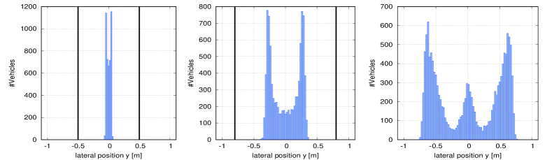
Figure 5: Simulation of the lateral distributions of lane-free dense bicycle traffic for path width 1.0 m (left), 1.6 m(middle), and 2.4 m(right).

Figure 6: Simulation of the trajectories of a 2.4 m wide lane-less bike path in $x$-$y$ direction (left) and in $x$-$t$ direction (right).

In Fig. 6, we take a closer look at the widest considered bikepath ($w=2.4\,\mathrm{m}$) where a third center file spontaneously begins to form. From $x=170\,\mathrm{m}$ to $x=200\,\mathrm{m}$, a bottleneck in form of a gradual width reduction to 1.6 m is introduced and the three-lane traffic spontaneously reorganizes into two-lane traffic, starting at $x=140\,\mathrm{m}$, i.e., 30 m upstream of the beginning of the bottleneck.

4 Discussion

The proposed Intelligent-agent model (IAM) integrates the continuous two-dimensional dynamics of the SFM with the high-speed properties of car-following models to which it reverts for single-lane traffic. The simulated anticipative high-speed behaviour of this model became most evident in the bicycle simulation of Fig. 6 where a spontaneous transition of three-lane to two-lane flow occurs 30 m upstream of the bottleneck. This anticipation is driven by the relative-speed term of the underlying IDM and can be observed for most longitudinal sub-models containing a relative-speed term. By construction, the SFM is not able to such an anticipation.

When adding floor fields, we obtain an integrated car-following and lane-changing model similar to MOBIL MOBIL-TRR07 ; traffic-simulation but with continuous lateral motion. We have shown that the IAM can describe the observed dynamics and emergent phenomena of mixed vehicular and motorcycle traffic and lane-free bicycle traffic. In the future, we plan to validate the model on further trajectory data, including truly lane-free mixed vehicular traffic Kanagaraj2018self and zipper merging and investigate microscopic aspects of the cyclist’s configuration and how the capacity depends on the path width wierbos2019capacity . For an online demonstration, see mtreiber.de/mixedTraffic/index.html.

References

- (1) M. Treiber, A. Kesting, Traffic Flow Dynamics: Data, Models and Simulation, Springer, Berlin, 2013.
- (2) M. Fellendorf, P. Vortisch, Microscopic traffic flow simulator vissim, in: Fundamentals of traffic simulation, Springer, 2010, pp. 63–93.
- (3) M. Behrisch, L. Bieker, J. Erdmann, D. Krajzewicz, Sumo-simulation of urban mobility-an overview, in: SIMUL 2011, The Third International Conference on Advances in System Simulation, 2011, pp. 55–60.
- (4) P. Hidas, Modelling lane changing and merging in microscopic traffic simulation, Transportation Research Part C: Emerging Technologies 10 (2002) 351–371.
- (5) A. Kesting, M. Treiber, D. Helbing, General lane-changing model MOBIL for car-following models, Transportation Research Record 1999 (2007) 86–94.
- (6) V. Kanagaraj, M. Treiber, Self-driven particle model for mixed traffic and other disordered flows, Physica A: Statistical Mechanics and its Applications 509 (2018) 1–11.
- (7) D. Helbing, P. Molnár, Social force model for pedestrian dynamics, Physical Review E 51 (1995) 4282–4286.
-
(8)
X. Chen, M. Treiber, V. Kanagaraj, H. Li, Social force models for pedestrian
traffic–state of the art, Transport reviews 38 (5) (2018) 625–653.
URL https://doi.org/10.1080/01441647.2017.1396265 - (9) G. Asaithambi, V. Kanagaraj, K. K. Srinivasan, R. Sivanandan, Study of traffic flow characteristics using different vehicle-following models under mixed traffic conditions, Transportation letters 10 (2) (2018) 92–103.
- (10) K. Madhu, K. K. Srinivasan, R. Sivanandan, Vehicle-following behaviour in mixed traffic–role of lane position and adjacent vehicle, Transportation Letters (2023) 1–14.
- (11) M. Treiber, A. Hennecke, D. Helbing, Congested traffic states in empirical observations and microscopic simulations, Physical Review E 62 (2000) 1805–1824.
- (12) M. Treiber, Interactive simulations of the intelligent driver model in combination with the lane-changing model mobil can be found at www.traffic-simulation.de (2022).
- (13) E. Barmpounakis, N. Geroliminis, On the new era of urban traffic monitoring with massive drone data: The pneuma large-scale field experiment, Transportation research part C: emerging technologies 111 (2020) 50–71.
- (14) M. J. Wierbos, V. L. Knoop, F. S. Hänseler, S. P. Hoogendoorn, Capacity, capacity drop, and relation of capacity to the path width in bicycle traffic, Transportation research record 2673 (5) (2019) 693–702.