Abstract

We investigate the effect of initial conditions on the fluctuations of the integrated density current across the origin ($x=0$) up to a given time $t$ in a one-dimensional system of non-interacting run-and-tumble particles. Each particle has initial probabilities $f^{+}$ and $f^{-}$ to move with an initial velocity $+v$ and $-v$ respectively, where $v>0$. We derive exact results for the variance (second cumulant) of the current for quenched and annealed averages over the initial conditions for the magnetization and the density fields associated with the particles. We show that at large times, the variance displays a $\sqrt{t}$ behavior, with a prefactor contingent on the specific density initial conditions used. However, at short times, the variance displays either linear $t$ or quadratic $t^{2}$ behavior, which depends on the combination of magnetization and density initial conditions, along with the fraction $f^{+}$ of particles in the positive velocity state at $t=0$. Intriguingly, if $f^{+}=0$, the variance displays a short time $t^{2}$ behavior with the same prefactor irrespective of the initial conditions for both fields.

 

Contents

1. 1 Introduction
2. 2 Microscopic model
   1. 2.1 Quenched and annealed averages
3. 3 Main results
4. 4 Single particle propagators
   1. 4.1 Symmetric initial bias velocity
   2. 4.2 Asymmetric initial bias velocity
5. 5 Current fluctuations for various initial conditions
   1. 5.1 Case 1: Annealed magnetization and annealed density initial conditions
   2. 5.2 Case 2: Quenched magnetization and annealed density initial conditions
   3. 5.3 Case 3: Quenched magnetization and quenched density initial conditions
   4. 5.4 Case 4: Annealed magnetization and quenched density initial conditions
6. 6 Conclusion and discussion
7. A General technique to find the Laplace transform of a function’s square
8. B Details of calculations

 

1 Introduction

Active systems are composed of self-propelling particles that consume energy at the individual level to perform directed motion [1, 2, 3, 4, 5, 6, 7, 8, 9, 10, 11, 12]. The breaking of detailed balance at the microscopic level allows such systems to exhibit behaviors that are distinct from equilibrium systems such as coherent motion, pattern formation, motility-induced phase separation (MIPS), amongst others [13, 14, 15, 16]. Particularly intriguing is the run and tumble (RTP) motion, employed by certain active particles, such as bacteria, to adeptly navigate their surroundings and explore their environment effectively [12, 17, 18, 19, 11, 10, 20, 21, 22, 23, 24]. During the running phase, bacteria move towards favorable conditions, while tumbling allows for random reorientation and exploration of new areas. Over the years, the RTP model has attracted significant attention leading to numerous studies on active particles such as first-passage properties, clustering and phase separation, large deviations, and collective motion [11, 17, 14, 25, 26, 27, 20, 21, 28].

In this work, we focus on the role of initial conditions on current fluctuations in a one-dimensional system comprising of run-and-tumble particles. To explore the effect of initial conditions on particle systems, two types of initial density profiles can be considered: (1) a deterministic profile in which the locations of particles are initially fixed (known as the “quenched density” setting), and (2) a random profile which has fluctuations in the initial positions (known as the “annealed density” setting). Active systems, on the other hand, also introduce an additional degree of freedom in the form of magnetization or polarization [14, 29, 30, 31, 32], which opens up the possibility of two more types of initial conditions: (3) a deterministic initial magnetization profile where the velocities of particles are fixed initially (termed “quenched magnetization” setting), and (4) a random initial profile which has fluctuations in the initial velocities of the particles (termed “annealed magnetization” setting).

The quantity of interest is the total number of particles $Q$, passing into the right side of the origin ($x>0$) up to time $t$. Numerous investigations have focused on the statistical properties of $Q$ in various passive systems, including random walkers, simple exclusion process (SEP), Kipnis-Marchioro-Presutti (KMP) model, amongst others using analytical methods like Bethe ansatz, Green’s function methods and macroscopic fluctuation theory (MFT) [33, 34, 35, 36, 37, 38, 39]. The effect of initial conditions on active systems has been first analyzed systematically in [40]. This study focused on a one-dimensional model of non-interacting RTPs, deriving an analytical expression for the variance of the integrated current $Q$ within the framework of annealed magnetization and annealed density. Later, this study was extended to incorporate the effect of quenched magnetization initial conditions in [41], focusing on step initial density and zero initial magnetization conditions. Current fluctuations in related models of run and tumble particle systems have also been analyzed in [32, 42]. In this study, we compute exact analytic expressions for the variance of $Q$ for general step initial conditions for both magnetization and density fields. This allows for a comparison between the fluctuations due to the differences in initial conditions for both fields at all times. We consider the case where all particles are initially distributed uniformly towards the left side of the origin ($x<0$). Each particle is associated with initial probabilities $f^{+}$ and $f^{-}$ to move with velocities $+v$ and $-v$, respectively, where $v>0$.

Through our analytical investigation, we find that at large times, the variance of the current displays a $\sqrt{t}$ behavior with a prefactor contingent on the specific density initial conditions used. This demonstrates that the fluctuations in the initial positions of particles have an everlasting effect on the fluctuations of $Q$, unlike the fluctuations in the initial velocities. However, at short times, the variance shows either a linear $t$ or a quadratic $t^{2}$ behavior influenced by the combination of initial conditions for both magnetization and density fields, as well as the fraction $f^{+}$ of particles with a positive velocity at $t=0$. A particularly intriguing observation is that when $f^{+}=0$, meaning there are no particles initially moving with a positive velocity, the variance displays a short time $t^{2}$ behavior. Interestingly, this behavior remains the same regardless of the initial conditions of the magnetization and density fields. Another intriguing aspect is the completely quenched situation in which both fields are quenched initially. In this case, the variance always exhibits a quadratic behavior at short times regardless of the values of $f^{+}$ and $f^{-}$. The specific scenario in which $f^{+}=f^{-}=1/2$ has been systematically examined in [41]. In this work, the scope of these results has been expanded to encompass arbitrary values of both $f^{+}$ and $f^{-}$.

This paper is organized as follows. In Sec. 2, we introduce the microscopic model and different averages used in the study. In Sec. 3, we provide an overview of the main results. We present derivations of the single particle propagators for various initial bias velocities in Sec. 4. In Sec. 5, we analytically compute the variance of $Q$ for different various averages over the magnetization and density fields. We present our conclusions from the study in Sec. 6. Finally, we provide details pertaining to some of the calculations in appendices A-B.

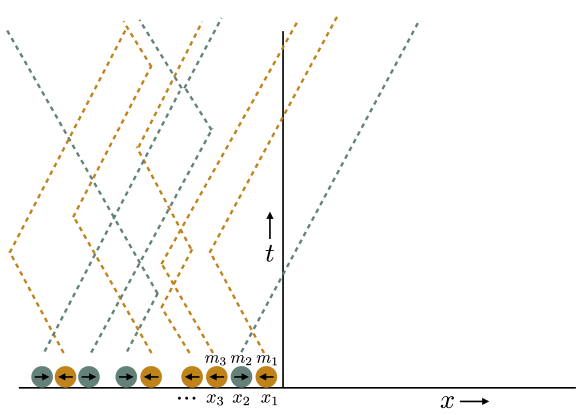
Figure 1: Schematic representation of the trajectories of non-interacting run and tumble particles. At time $t=0$, all particles are uniformly distributed towards the left of the origin. The label $m_{i}({x_{i}})$ indicates the initial velocity(position) of the $i^{\text{th}}$ particle. Different colors denote particles with different initial bias velocities.

2 Microscopic model

We consider a box confined within the interval $\left[-L,0\right]$ in one dimension with $N$ run and tumble particles. The dynamics of each particle evolve according to the following Langevin equation

$$\frac{\partial x_{i}(t)}{\partial t}=vm_{i}(t),~{}1<i<N,$$ (1)

where $v>0$. The stochastic variable $m_{i}(t)$ alternates between the values of $+1$ and $-1$ at a fixed rate . The $i{\text{th}}$ particle has a bias velocity $\pm v$ at time $t$ for $m_{i}(t)=\pm 1$, . If the initial velocity of a particle is $+v$, then the particle is in $+$ state, and if the initial velocity is $-v$, then the particle is in $-$ state. This velocity behaves akin to an internal spin state, leading us to construct a magnetization field corresponding to the active motion of the particles. We introduce a density field linked to the positions, denoted as $\rho(x,t)=\sum_{i=1}^{N}\delta(x-x_{i}(t))/L$, and a magnetization field, expressed as $m(x,t)=\sum_{i=1}^{N}\delta(x-x_{i}(t))m_{i}(t)/L$, related to the velocities of these active particles. We consider a step initial density condition where particles are evenly distributed on the left side of the origin ($x<0$) with density , i.e. $\rho(x,0)=\theta(-x)\rho$ with $\rho=N/L$ as the number of particles per unit length and as the Heaviside step function. Let $f^{+}$ denote the fraction of particles with $+v$ velocity and $f^{-}$ denote the fraction of particles with $-v$ velocity at time $t=0$, with $f^{+}+f^{-}=1$. This yields a step initial magnetization condition, $m(x,0)=(f^{+}-f^{-})\theta(-x)\rho$. For $f^{+}=f^{-}=1/2$, $m(x,0)=0$, and this model reduces to the model studied in [40, 41]. Even though we start with a finite-dimensional box, we eventually take the thermodynamic limit of $N\rightarrow\infty,~{}L\rightarrow\infty$ with $N/L\rightarrow\rho$ fixed in our analytical calculations.

We examine the statistical behavior of the total number of particles, represented as $Q$, traversing the origin within a given time frame $t$. As an RTP traverses the origin from the left to the right, it adds a positive value of $+1$ to the overall current. Conversely, when it moves from the right to the left, it contributes a negative value of $-1$ to the current. Thus, the integrated current $Q$ across the origin up to time $t$ is equivalent to the total number of particles towards the right side of the origin at that specific time $t$. We provide a schematic representation of the dynamics of the particles in Fig. 1. We next elucidate the various types of averages that can be utilized to examine how the fluctuations of $Q$ are influenced by the initial conditions.

2.1 Quenched and annealed averages

We consider various types of averages involving the initial velocities and positions of particles to study the effect of initial conditions on the fluctuations of $Q$. The initial velocities(positions) remain fixed in the quenched magnetization(density) setting. However, the initial velocities(positions) of the particles are allowed to fluctuate in the annealed magnetization(density) setting. We denote the initial velocities of particles by $\{m_{i}\}$ and the initial positions by $\{x_{i}\}$. The symbol $\langle\cdots\rangle_{\{m_{i}\},\{x_{i}\}}$ represents an ensemble average over the history of realizations, considering fixed initial velocities and positions of particles. We also use two additional averages, denoted by $\overbrace{\cdots}$ for an average over initial particle velocities and $\overline{\cdots}$ for an average over initial particle positions.

Let us represent by $P_{a,a}(Q,t)$ the probability distribution of $Q$ where both initial velocities and positions are subjected to fluctuations. The initial conditions for velocities and positions are denoted by the first and second subscripts respectively where “$q$" stands for quenched and “$a$" stands for annealed scenarios. For this annealed magnetization and annealed density setting, the moment-generating function can be computed as

$$\sum_{Q=0}^{\infty}e^{-kQ}P_{a,a}(Q,t)=\overbrace{\overline{\langle e^{-kQ}\rangle_{\{m_{i}\},\{x_{i}\}}}}.$$ (2)

We next consider the case where at time $t=0$, one fixes the velocities of the particles, but the positions of the particles are allowed to fluctuate. The distribution of $Q$ for this scenario is represented by $P_{q,a}(Q,t)$ and the corresponding moment-generating function is expressed as

$$\sum_{Q=0}^{\infty}e^{-kQ}P_{q,a}(Q,t)=e^{\overbrace{\ln\overline{\langle e^{-kQ}\rangle_{\{m_{i}\},\{x_{i}\}}}}}.$$ (3)

For the case where both initial particle velocities and positions are fixed, the flux distribution is labeled as $P_{q,q}(Q,t)$. In this case, the moment-generating function can be expressed as

$$\sum_{Q=0}^{\infty}e^{-kQ}P_{q,q}(Q,t)=e^{\overbrace{\overline{\ln\langle e^{-kQ}\rangle_{\{m_{i}\},\{x_{i}\}}}}}.$$ (4)

Finally, we consider the case where the velocities of the particles are subject to fluctuations, but the positions of the particles are held constant at $t=0$. The resulting distribution of $Q$ is labeled by $P_{a,q}(Q,t)$ and the expression for the moment-generating function associated with this case is given by

$$\sum_{Q=0}^{\infty}e^{-kQ}P_{a,q}(Q,t)=e^{\overline{\ln\overbrace{\langle e^{-kQ}\rangle_{\{m_{i}\},\{x_{i}\}}}}}.$$ (5)

3 Main results

$t\rightarrow 0$	$t\rightarrow\infty$
$\rho vf^{+}t-\frac{\rho v\gamma}{4}\left(3f^{+}-f^{-}\right)t^{2}$	$\rho\sqrt{\frac{{D_{\text{eff}}}~{}{t}}{{\pi}}}$	${}_{a,a}^{2}(t)$
$\rho vf^{+}t-\frac{\rho v\gamma}{4}\left(3f^{+}-f^{-}\right)t^{2}$	$\rho\sqrt{\frac{{D_{\text{eff}}}~{}{t}}{{\pi}}}$	${}_{q,a}^{2}(t)$
$\frac{\rho v\gamma}{4}\left(3f^{+}+f^{-}\right)t^{2}$	$\rho\sqrt{\frac{{D_{\text{eff}}}~{}{t}}{{2\pi}}}$	${}_{q,q}^{2}(t)$
$\rho v{f^{+}f^{-}}t+\frac{\rho v\gamma}{4}\left(3f^{+}-f^{-}\right)\left(f^{+}-f^{-}\right)t^{2}$	$\rho\sqrt{\frac{{D_{\text{eff}}}~{}{t}}{{2\pi}}}$	${}_{a,q}^{2}(t)$

Table 1: Asymptotic behaviors of the variance ${}^{2}(t)$ of the integrated current for different initial conditions. The initial conditions for magnetization and density fields are denoted by the first and second subscripts respectively where “$a$" stands for annealed and “$q$" stands for quenched scenarios. Here, $D_{\text{eff}}=v^{2}/(2\gamma)$ is the effective diffusion constant for RTP motion in one dimension. The mean of $Q$ denoted as $\mu(t)$ is equal to ${}_{a,a}^{2}(t)={}_{q,a}^{2}(t)$ and is the same for all initial conditions.

We focus on the role of initial conditions on the fluctuations of the integrated current $Q$. The mean of $Q$ takes on the same characteristics regardless of the specific initial conditions [36]. However, the variance displays interesting differences for various averages involving the initial conditions. We first examine the situation where both initial velocities and positions of particles can fluctuate, referred to as the annealed magnetization and annealed density setting. An equivalent situation is the quenched magnetization and annealed density setting, in which velocities remain fixed initially while positions are subject to fluctuations [41]. In the infinite system size limit, the distributions of $Q$ for both these initial conditions become identical. This is due to the fact that whether the velocities are kept constant or allowed to fluctuate makes no difference, given that the initial positions of particles are subjected to fluctuations. Therefore, the fluctuations in the initial velocities do not have any effect on the distribution of $Q$ (and hence the variance) when the initial positions are random. The exact analytical form for the variance of $Q$ in both these scenarios can be computed as

$${}_{a,a}^{2}(t)={}_{q,a}^{2}(t)=\frac{\rho v}{4\gamma}\left[2\gamma te^{-\gamma t}\left(\boldsymbol{I}_{0}(\gamma t)+\boldsymbol{I}_{1}(\gamma t)\right)+\left(f^{+}-f^{-}\right)\left(1-e^{-2\gamma t}\right)\right].$$ (6)

As before, the initial conditions for magnetization and density fields are denoted by the first and second subscripts respectively where “$q$" stands for quenched and “$a$" stands for annealed scenarios. The symbols $\boldsymbol{I}_{0}$ and $\boldsymbol{I}_{1}$ denote modified Bessel functions of order $0$ and $1$ respectively. The modified Bessel function $\boldsymbol{I}_{n}(z)$ of order $n$ is a solution to the homogeneous Bessel differential equation $z^{2}y^{{}^{\prime\prime}}(z)+zy^{{}^{\prime}}(z)-(z^{2}+n^{2})y=0$. The expression in Eq. (6) is also the same as the mean for various initial conditions. When $f^{+}=f^{-}=1/2$, we obtain the simplified expression [40, 41]

$${}_{a,a}^{2}(t)={}_{q,a}^{2}(t)=\frac{\rho v}{2}te^{-\gamma t}(\boldsymbol{I}_{0}(\gamma t)+\boldsymbol{I}_{1}(\gamma t)),~{}\text{for}~{}f^{+}=f^{-}=1/2.$$ (7)

This is the specific case studied in [40, 41].

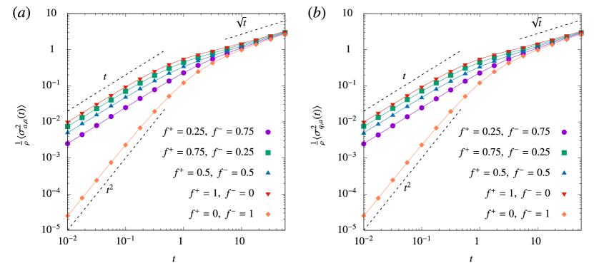
Figure 2: Variance of the time integrated current $Q$ plotted as a function of time $t$ for different values of $f^{+}$ and $f^{-}$. The specific cases displayed are (a) annealed magnetization and annealed density initial conditions (b) quenched magnetization and annealed density initial conditions. The points are obtained from direct numerical simulations and the solid curves correspond to the exact analytical result in Eq. (6). These plots are for the parameter values $\rho=20,~{}\gamma=1,~{}v=1$. We notice that the variance exhibits similar behavior for both quenched and annealed magnetization initial conditions.

We examine a third scenario, which involves quenching the initial magnetization and density fields, meaning the initial particle velocities and positions are fixed. For this non-trivial case, the exact expression for the variance in real time is hard to compute. Nevertheless, it is possible to calculate the exact analytic expression in Laplace space. We define the Laplace transform of a general function $f(t)$ as $\mathcal{L}\left[f(t)\right]=\tilde{f}(s)=\int_{0}^{\infty}e^{-st}f(t)dt$. We show that

$$\tilde{\sigma}_{q,q}^{2}(s)=\rho\left[\frac{v\gamma}{s(s+2\gamma)\sqrt{s(s+4\gamma)}}+\frac{(f^{+}-f^{-})v}{4\pi s(s+2\gamma)}\left({\pi-2K\left(-{8\gamma(s+2\gamma)}/{s^{2}}\right)}\right)\right].$$ (8)

In the above equation, $K$ is the elliptic integral of the first kind defined as

$$K(n)=\int_{0}^{\frac{\pi}{2}}\left({1}/{\sqrt{1-n~{}{\sin}^{2}\theta}}\right)d\theta.$$ (9)

Equation (8) can be used to extract the asymptotic behaviors of the variance in real-time and is given in Table 1. Additionally, for symmetric initial conditions with $f^{+}=f^{-}=1/2$, this expression can be inverted exactly yielding [41]

$${}_{q,q}^{2}(t)=\frac{\rho v}{4}e^{-2\gamma t}t\left[(2+\pi\boldsymbol{L}_{0}(2\gamma t))\boldsymbol{I}_{1}(2\gamma t)-\pi\boldsymbol{L}_{1}(2\gamma t)\boldsymbol{I}_{0}(2\gamma t)\right],~{}\text{for}~{}f^{+}=f^{-}=1/2,$$ (10)

where the symbols $\boldsymbol{L}_{0}$ and $\boldsymbol{L}_{1}$ denote modified Struve functions of order $0$ and $1$ respectively. The modified Struve function $\boldsymbol{L}_{n}(z)$ of order $n$ is a solution to the non-homogeneous Bessel differential equation $z^{2}y^{{}^{\prime\prime}}(z)+zy^{{}^{\prime}}(z)-(z^{2}+n^{2})y={4{\left({z}/{2}\right)}^{n+1}}/{\left(\sqrt{\pi}~{}\Gamma(n+\frac{1}{2})\right)}$ where is the gamma function.

The last scenario we investigate involves annealed magnetization and quenched density, in which the particle positions are fixed, however, their velocities are permitted to fluctuate initially. The exact analytic expression for the Laplace transform of the variance can be obtained as

$$\tilde{\sigma}_{a,q}^{2}(s) = \frac{\rho v}{s^{3/2}(s+2\gamma)}\Bigg{[}\frac{1}{2}\sqrt{s}\left(f^{+}-f^{-}\right)+\left(\frac{\gamma}{\sqrt{s+4\gamma}}-\frac{1}{2}\sqrt{s+2\gamma}\right)\left({f^{+}}^{2}+{f^{-}}^{2}\right)$$ (11)

$$- \left(\frac{2\gamma}{\sqrt{s+4\gamma}}+\sqrt{s+2\gamma}-\sqrt{s+4\gamma}\right)f^{+}f^{-}+\frac{\sqrt{s+2\gamma}}{2}$$

$$- \sqrt{s}\left(\frac{K\left(-{8\gamma(s+2\gamma)}/{s^{2}}\right)}{2\pi}+\frac{1}{4}\right)\left({f^{+}}^{2}-{f^{-}}^{2}\right)\Bigg{]}.$$

For symmetric initial conditions $f^{+}=f^{-}=1/2$, the above expression can be inverted exactly yielding [41]

$${}_{a,q}^{2}(t)=\frac{\rho v}{8}e^{-2\gamma t}t\left[(4+\pi\boldsymbol{L}_{0}(2\gamma t))\boldsymbol{I}_{1}(2\gamma t)+(2-\pi\boldsymbol{L}_{1}(2\gamma t))\boldsymbol{I}_{0}(2\gamma t)\right],$$

$$~{}\text{for}~{}f^{+}=f^{-}=1/2.$$ (12)

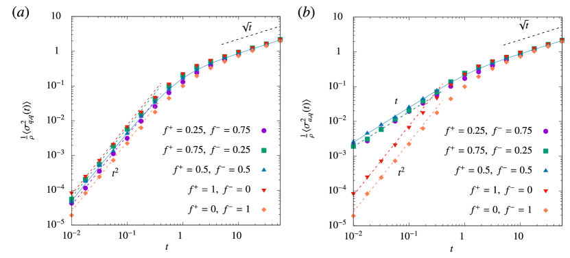
Figure 3: Variance of the time integrated current $Q$ plotted as a function of time $t$ for different values of $f^{+}$ and $f^{-}$. The specific cases displayed are (a) quenched magnetization and quenched density initial conditions (b) annealed magnetization and quenched density initial conditions. The points are obtained from direct numerical simulations. The solid curves for $f^{+}=f^{-}=1/2$ in (a) and (b) correspond to the exact analytical results in Eqs. (10) and (12) respectively. The dashed curves correspond to the asymptotic behaviors listed in Table 1. These plots are for the parameter values $\rho=20,~{}\gamma=1,~{}v=1$.

The asymptotic behaviors of the variance for each of the four cases discussed above are listed in Table 1. We also compare our analytical predictions for the variance of $Q$ with direct Monte Carlo simulations in Fig. 2 and Fig. 3. Our theoretical predictions align remarkably well with the results obtained from Monte Carlo simulations.

We notice from Table 1 that for the special case where $f^{+}=0$ and $f^{-}=1$, the mean and the variance always grow as ${\rho v\gamma t^{2}}/{4}$ in the small time limit irrespective of the initial conditions. The behavior of the mean can be understood as explained below. Consider a single run and tumble particle starting from the location $-x_{0}$ with $x_{0}>0$ at time $t=0$ in $-$ state (i.e. with velocity $-v$). The particle cannot cross the origin until it flips the velocity state. At short times, we can safely approximate that the mean is dominated by trajectories with a single flip. Let be the time taken by the particle to flip its velocity state. Here, is a stochastic variable. For the particle to be able to cross the origin within a time $t>\tau$, the necessary condition is

$$x_{0}+\tau v<(t-\tau)v.$$ (13)

That is, the distance to the location of the particle just before the first flip (before time ) should be less than the distance traveled by the particle in the remaining time interval $t-\tau$. Equation (13) can be rewritten as

$$\tau<\frac{1}{2}\left(t-\frac{x_{0}}{v}\right).$$ (14)

Since the distribution of the time gap between consecutive flips is Poissonian, the probability that the particle will cross the origin within a time $t$ is given as

$$\langle Q(t)|x_{0}\rangle=\int_{0}^{\frac{1}{2}\left(t-\frac{x_{0}}{v}\right)}\gamma e^{-\gamma\tau}d\tau=1-e^{-\frac{\gamma}{2}\left(t-\frac{x_{0}}{v}\right)}.$$ (15)

If the density of particles is , the average current is then given as

$$\langle Q\rangle=\rho\int_{0}^{vt}\left(1-e^{-\frac{\gamma}{2}\left(t-\frac{x_{0}}{v}\right)}\right)dx_{0}=\rho v\left(t-\frac{2\left(1-e^{-\frac{1}{2}\gamma t}\right)}{\gamma}\right),$$ (16)

which in the short time limit yields

$$\langle Q\rangle\xrightarrow[t\rightarrow 0]{}\frac{\rho v\gamma}{4}t^{2}.$$ (17)

In Sec. 5, we demonstrate that when the initial density conditions are annealed, the flux distribution consistently follows a Poisson distribution. This holds regardless of the initial magnetization conditions. Therefore, both $P_{a,a}(Q,t)$ and $P_{q,a}(Q,t)$ are Poissonian, as evidenced by Eqs. (65) and (72), respectively. Consequently, the mean value of the distribution is equal to its variance in these cases. Hence, the result presented in Eq. (17) also applies to the variance when the initial density conditions are annealed. This finding aligns with the limiting behaviors outlined in Table 1, considering the parameter choice of $f^{+}=0$ and $f^{-}=1$. We also note that for initial conditions in which both magnetization and density fields are quenched, the variance consistently follows a short-time quadratic $t^{2}$ behavior, regardless of the specific values of $f^{+}$ and $f^{-}$.

4 Single particle propagators

In this section, we derive expressions for the single particle propagators in one dimension associated with a run and tumble particle (RTP). We also provide expressions for the integrals of these Green’s functions. These expressions will be useful in the analytical calculations presented in the next section. We consider symmetric and asymmetric initial bias velocities separately. An alternate method to derive the single particle propagators has also been given in [41].

We consider a single run and tumble particle starting from the position $x=0$ initially. We use the notation $P_{m}(x,t)$ to represent the probability density of the RTP to be at position $x$ at time $t$. The subscript ‘$m$’ represents the velocity state of the particle at time $t$ which can either be $+$ or $-$. The evolution equations for this quantity can be written as [17]

$$\frac{\partial P_{+}(x,t)}{\partial t}+v\frac{\partial P_{+}(x,t)}{\partial x}+\gamma P_{+}(x,t)-\gamma P_{-}(x,t)=0,$$

$$\frac{\partial P_{-}(x,t)}{\partial t}-v\frac{\partial P_{-}(x,t)}{\partial x}+\gamma P_{-}(x,t)-\gamma P_{+}(x,t)=0.$$ (18)

The combined occupation probability is given by $P(x,t)=P_{-}+P_{+}$. After performing a Laplace transform of Eq. (18), we obtain

$$-P_{+}(x,0)+v\frac{\partial\tilde{P}_{+}(x,s)}{\partial x}+(s+\gamma)\tilde{P}_{+}(x,s)-\gamma\tilde{P}_{-}(x,s) = 0,$$

$$-P_{-}(x,0)-v\frac{\partial\tilde{P}_{-}(x,s)}{\partial x}+(s+\gamma)\tilde{P}_{-}(x,s)-\gamma\tilde{P}_{+}(x,s) = 0.$$ (19)

We consider an ansatz of the form

$$\tilde{P}_{\pm}=A_{\pm}{\rm e^{-\beta x}}\quad\mbox{for}\quad x>0,$$

$$\tilde{P}_{\pm}=B_{\pm}{\rm e^{+\beta x}}\quad\mbox{for}\quad x<0.$$ (20)

Substituting these solutions into Eq. (19) (away from $x=0$) yields

$$(s+\gamma-\beta v)A_{+}=\gamma A_{-},$$

$$(s+\gamma+\beta v)B_{+}=\gamma B_{-},$$

$$(s+\gamma+\beta v)A_{-}=\gamma A_{+},$$

$$(s+\gamma-\beta v)B_{-}=\gamma B_{+}.$$ (21)

Combining the above equations yields the expression for as

$$\beta=\frac{\sqrt{s(s+2\gamma)}}{v}.$$ (22)

Since the total probability $P$ has to be normalized, we obtain the condition

$$\int_{-\infty}^{\infty}\left(\tilde{P}_{+}+\tilde{P}_{-}\right)dx=\frac{1}{s}.$$ (23)

This implies

$$A_{+}+A_{-}+B_{+}+B_{-}=\frac{\beta}{s}.$$ (24)

This condition along with the initial conditions can be together used to evaluate the undetermined coefficients $A_{\pm}$ and $B_{\pm}$ as we demonstrate in the following subsections. We consider symmetric and asymmetric initial bias velocities separately.

4.1 Symmetric initial bias velocity

We consider symmetric initial bias velocities of the form

$$P_{-}(x,0)=\frac{\delta(x)}{2},~{}P_{+}(x,0)=\frac{\delta(x)}{2}.$$ (25)

This means that the particle can start from either $+$ or $-$ velocity state with equal probability. Integrating Eq. (19) over $x$ yields

$$-\frac{1}{2}+\frac{(s+\gamma)}{\beta}(A_{+}+B_{+})-\frac{\gamma}{\beta}(A_{-}+B_{-})=0,$$

$$-\frac{1}{2}+\frac{(s+\gamma)}{\beta}(A_{-}+B_{-})-\frac{\gamma}{\beta}(A_{+}+B_{+})=0.$$ (26)

Solving Eqs. (21), (24) and (26) yields the expressions for coefficients as

$$A_{+}=\frac{v\beta+s}{4sv}, A_{-}=\frac{v\beta-s}{4sv},$$

$$B_{+}=\frac{v\beta-s}{4sv}, B_{-}=\frac{v\beta+s}{4sv}.$$ (27)

Using the above expressions and the form of ansatz provided in Eq. (20), we directly obtain [40]

$$\tilde{P}(x,s)=\frac{\beta e^{-\beta|x|}}{2s},$$ (28)

where is given in Eq. (22).

We define the symmetric Green’s function $G^{0}(x,x_{i},t)$ as the probability density of locating a run and tumble particle at position $x$ at time $t$, given that it started from position $x_{i}$ at time $t=0$, with an equal chance of being in the $+$ or $-$ state. We use the superscript $``0"$ to indicate the symmetric scenario in which the RTP starts from $+$ or $-$ state with equal probability. Due to the translational invariance of the evolution equations, Eqs. (28) and (22) directly lead to

$$\tilde{G}^{0}(x,-z,s) = \frac{\sqrt{s(s+2\gamma)}e^{-\frac{\sqrt{s(s+2\gamma)}\left|x+z\right|}{v}}}{2vs},\quad z=-x_{i}.$$ (29)

For step initial conditions, we consider $x_{i}\leq 0$, thus $z\geq 0$.

We define the integral of $G^{0}(x,-z,t)$ from $x=0$ to $\infty$ as

$$M^{0}(z,t)=\int_{0}^{\infty}G^{0}(x,-z,t)dx.$$ (30)

The quantity $M^{0}(z,t)$ corresponds to the probability that a particle starting from the position $-z$ in a symmetrized velocity state is found towards the right side of the origin at time $t$. Using the exact expression in Eq. (29), we derive the Laplace transform of $M^{0}(z,t)$ as

$$\tilde{M}^{0}(z,s) = \frac{\exp\left(-\frac{\sqrt{s(s+2\gamma)}z}{v}\right)}{2s}.$$ (31)

We next integrate the function $\tilde{M}^{0}(z,s)$ over the variable $z$ to yield

$$\int_{0}^{\infty}\tilde{M}^{0}(z,s)dz=\frac{v}{2s^{3/2}\sqrt{(s+2\gamma)}}.$$ (32)

We then introduce the Laplace transform of $M^{0}(z,t)^{2}$, denoted as

$$\tilde{W}^{0}(z,s)=\mathcal{L}\left[{M^{0}(z,t)}^{2}\right].$$ (33)

This quantity proves valuable in the calculations of the current fluctuations detailed in the subsequent section. Integrating the function $\tilde{W}^{0}(z,s)$ over $z$ results in

$$\int_{0}^{\infty}\tilde{W}^{0}(z,s)dz=\frac{v}{2s^{3/2}}\left(\frac{2(s+2\gamma)-\sqrt{s+4\gamma}\sqrt{s+2\gamma}}{2(s+2\gamma)^{3/2}}\right).$$ (34)

We provide details regarding the calculation of the above integral in Appendix B.

4.2 Asymmetric initial bias velocity

Next, we examine scenarios with asymmetric initial bias velocities, where the particle is initially placed in either the $+$ or $-$ state.

Case 1: RTP initialized in the $+$ state:

We investigate the asymmetric initial conditions

$$P_{-}(x,0)=0,\quad P_{+}(x,0)=\delta(x).$$ (35)

In this case, the RTP starts its motion from the $+$ velocity state initially. Integrating Eq. (19) over $x$ yields

$$-1+\frac{(s+\gamma)}{\beta}(A_{+}+B_{+})-\frac{\gamma}{\beta}(A_{-}+B_{-}) = 0,$$

$$\frac{(s+\gamma)}{\beta}(A_{-}+B_{-})-\frac{\gamma}{\beta}(A_{+}+B_{+}) = 0.$$ (36)

Solving Eqs. (21), (24) and (36) yields the expressions for coefficients as

$$A_{+}=\frac{s+\gamma+v\beta}{2v^{2}\beta}, A_{-}=\frac{\gamma}{2v^{2}\beta},$$

$$B_{+}=\frac{s+\gamma-v\beta}{2v^{2}\beta}, B_{-}=\frac{\gamma}{2v^{2}\beta}.$$ (37)

Using the above expressions and the form of ansatz provided in Eq. (20), we obtain

$$\tilde{P}(x,s)=\frac{\left(\beta+\text{sign}(x)\frac{s}{v}\right)}{2s}{{\rm e}^{-\beta|x|}},$$ (38)

where the expression for is provided in Eq. (22) and sign is the sign function.

Case 2: RTP initialized in the $-$ state:

Here, we consider the asymmetric initial conditions

$$P_{+}(x,0)=0,\quad P_{-}(x,0)=\delta(x).$$ (39)

In this case, the RTP starts its motion from the $-$ velocity state initially. Integrating Eq. (19) over $x$ yields

$$\frac{(s+\gamma)}{\beta}(A_{+}+B_{+})-\frac{\gamma}{\beta}(A_{-}+B_{-}) = 0,$$

$$-1+\frac{(s+\gamma)}{\beta}(A_{-}+B_{-})-\frac{\gamma}{\beta}(A_{+}+B_{+}) = 0.$$ (40)

Solving Eqs. (21), (24) and (40) yields the expressions for coefficients as

$$A_{+}=\frac{\gamma}{2v^{2}\beta}, A_{-}=\frac{s+\gamma-v\beta}{2v^{2}\beta},$$

$$B_{+}=\frac{\gamma}{2v^{2}\beta}, B_{-}=\frac{s+\gamma+v\beta}{2v^{2}\beta}.$$ (41)

Using the above expressions, we obtain

$$\tilde{P}(x,s)=\frac{\left(\beta-\text{sign}(x)\frac{s}{v}\right)}{2s}{\rm e}^{-\beta|x|},$$ (42)

where is given in Eq. (22).

We next introduce the asymmetric Green’s functions $G^{\pm}(x,x_{i},t)$, which represent the probability density of finding a run and tumble particle at position $x$ at time $t$, given that it started from position $x_{i}$ initially, in a fixed bias state $\pm$. The asymmetric scenario is denoted by the superscript $``\pm"$. Using translational symmetry and combining Eqs. (42), (38) and (22), we obtain

$$\tilde{G}^{\pm}(x,-z,s) = \frac{\left(\sqrt{s(s+2\gamma)}\pm s~{}\text{sign}(x+z)\right)}{2vs}e^{-\frac{\sqrt{s(s+2\gamma)}\left|x+z\right|}{v}},\quad z=-x_{i},$$ (43)

in which sign denotes the sign function.

We next define the integral of $G^{\pm}(x,-z,t)$ over $x>0$ as

$$M^{\pm}(z,t)=\int_{0}^{\infty}G^{\pm}(x,-z,t)dx.$$ (44)

The quantity $M^{\pm}(z,t)$ corresponds to the probability that a particle starting from the location $-z$ in the velocity state $\pm$ is found towards the right side of the origin at time $t$. Using Eq. (43) and the definition provided in Eq. (44), we derive the analytic expression for the Laplace transform of $M^{\pm}(z,t)$ as

$$\tilde{M}^{\pm}(z,s) = \left(\frac{1}{2s}\pm\frac{1}{2\sqrt{s(s+2\gamma)}}\right){e^{-\frac{\sqrt{s(s+2\gamma)}z}{v}}}.$$ (45)

We integrate $\tilde{M}^{\pm}(z,s)$ over $z$ to yield

$$\int_{0}^{\infty}\tilde{M}^{\pm}(z,s)dz=\frac{v\left(\sqrt{s(s+2\gamma)}\pm s\right)}{2s^{2}(s+2\gamma)}.$$ (46)

We introduce

$$\tilde{W}^{\pm}(z,s)=\mathcal{L}\left[{M^{\pm}(z,t)}^{2}\right],$$ (47)

as the Laplace transform of $M^{\pm}(z,t)^{2}$. After performing some algebraic calculations (details are presented in Appendix B), we show

$$\int_{0}^{\infty}\tilde{W}^{\pm}(z,s)dz=\frac{v}{2s(s+2\gamma)}\left(\pm\frac{1}{2}+\sqrt{\frac{s+2\gamma}{s}}-\frac{2\gamma}{\sqrt{s(s+4\gamma)}}\pm\frac{K\left(-{8\gamma(s+2\gamma)}/{s^{2}}\right)}{\pi}\right).$$ (48)

Another important quantity involved in the calculations of current fluctuations is the Laplace transform of the product of $M^{-}(z,t)$ and $M^{+}(z,t)$. We denote

$$\tilde{W}^{\text{prod}}(z,s)=\mathcal{L}\left[M^{-}(z,t)M^{+}(z,t)\right].$$ (49)

As the symmetric propagator $G^{0}$ is the average of the asymmetric propagators $G^{-}$ and $G^{+}$, we have

$$G^{0}(x,x_{i},t)=\left(G^{-}(x,x_{i},t)+G^{+}(x,x_{i},t)\right)/2,$$ (50)

and consequently

$$M^{0}(z,t)=\left(M^{-}(z,t)+M^{+}(z,t)\right)/2.$$ (51)

Using Eqs. (33), (47), and (51) we obtain

$$\tilde{W}^{\text{prod}}(z,s)=2\tilde{W}^{0}(z,s)-\frac{1}{2}\left(\tilde{W}^{-}(z,s)+\tilde{W}^{+}(z,s)\right).$$ (52)

After performing the integration over $z$ and plugging in the expressions given in Eqs. (34) and (48), we obtain

$$\int_{0}^{\infty}\tilde{W}^{\text{prod}}(z,s)dz=\frac{v}{\sqrt{s}(s+2\gamma)^{3/2}}\left(\frac{s+\gamma}{2s}+\frac{\gamma\sqrt{\frac{s(s+2\gamma)}{s+4\gamma}}}{s^{3/2}}-\frac{\sqrt{s(s+2\gamma)(s+4\gamma)}}{2s^{3/2}}\right).$$ (53)

5 Current fluctuations for various initial conditions

In this section, we analytically compute the variance of the current $Q$ for different initial conditions involving the magnetization and density fields. Let ${m_{i}}$ represent the initial velocities or bias states of particles and ${x_{i}}$ represent the initial positions. The positions $x_{i}$s are selected uniformly from the interval $-L$ to $0$. In this context, $i\in[1,N]$ denote the particle index with $x_{i}<0$. The initial velocity states of the particles $m_{i}$s can either be $+$ with a probability of $f^{+}$ or $-$ with a probability of $f^{-}$, where $f^{+}+f^{-}=1$. Thus $f^{+}$ and $f^{-}$ denote the fraction of positive and negative biased particles respectively at time $t=0$.

We follow similar steps introduced in [40, 41] to compute the current fluctuations for different initial conditions. Let ${\cal I}_{i}(t)$ be an indicator function defined as

$${\cal I}_{i}(t)=\begin{cases}1,&\text{if at time $t$, the $i{\text{th}}$ particle is towards the right side of the origin },\\ 0,&\text{otherwise}.\end{cases}$$ (54)

The total number of particles $N^{+}$ to the right side of the origin is thus given as

$$N^{+}=\sum_{i=1}^{N}{\cal I}_{i}(t).$$ (55)

As mentioned before, the total number of particles that cross the origin within time $t$ is equivalent to the number of particles situated to the right of the origin at time $t$. For a fixed initial realization of the bias states $\{m_{i}\}$ and the positions $\{x_{i}\}$, the distribution of $Q$ is given as

$$P(Q,t,\{m_{i}\},\{x_{i}\})={\rm Prob.}~{}(N^{+}=Q)=\left\langle\delta\left[Q-\sum_{i=1}^{N}{\cal I}_{i}(t)\right]\right\rangle_{\{m_{i}\},\{x_{i}\}}.$$ (56)

Here, the angular bracket $\langle\cdots\rangle_{\{m_{i}\},\{x_{i}\}}$ represents an average over the history of realizations, while keeping the bias states $\{m_{i}\}$ and the initial positions $\{x_{i}\}$ fixed.

We next turn to the computation of the generating function of $Q$. Multiplying Eq. (56) with $e^{-kQ}$ and summing over $Q$ yield

$$\sum_{Q=0}^{\infty}e^{-kQ}P(Q,t,\{m_{i}\},\{x_{i}\})=\langle e^{-kQ}\rangle_{\{m_{i}\},\{x_{i}\}}=\left\langle\exp[{-k\sum_{i=1}^{N}{\cal I}_{i}(t)}]\right\rangle_{\{m_{i}\},\{x_{i}\}}.$$ (57)

Since we focus on a non-interacting process, the motion of each particle can be considered independently. We have the identity $e^{-k{\cal I}_{i}}=1+(e^{-k}-1){\cal I}_{i}$ because the indicator variable ${\cal I}_{i}$ can only take values $0$ or $1$. Inserting this identity in Eq. (57) and considering the non-interacting nature of particle motion yield

$$\langle e^{-kQ}\rangle_{\{m_{i}\},\{x_{i}\}}=\prod_{i=1}^{N}\left[1+(e^{-k}-1)\langle{\cal I}_{i}(t)\rangle_{\{m_{i}\},\{x_{i}\}}\right].$$ (58)

The average $\langle{\cal I}_{i}(t)\rangle_{\{m_{i}\},\{x_{i}\}}$ is the probability that the $i$th particle starting from the position $x_{i}$ in the velocity state $m_{i}$ is present on the right side of the origin at a later time $t$. This quantity is connected to the single particle propagator $G^{m_{i}}(x,x_{i},t)$ as

$$\langle{\cal I}_{i}(t)\rangle_{\{m_{i}\},\{x_{i}\}}=\int_{0}^{\infty}G^{m_{i}}(x,x_{i},t)dx=M^{m_{i}}(-x_{i},t),\quad x_{i}<0.$$ (59)

After inserting Eq. (59) into Eq. (58), we obtain

$$\langle e^{-kQ}\rangle_{\{m_{i}\},\{x_{i}\}}=\prod_{i=1}^{N}\left[1+(e^{-k}-1)M^{m_{i}}(-x_{i},t)\right],\quad x_{i}<0.$$ (60)

As specified before, $\overbrace{\cdots}$ denotes an average over the initial particle velocities and $\overline{\cdots}$ denotes an average over the initial particle positions. In the following subsections, we consider the effect of these averages separately.

5.1 Case 1: Annealed magnetization and annealed density initial conditions

In this section, we consider an initial condition where the initial bias states and positions of particles are allowed to fluctuate. The corresponding flux distribution is labeled as $P_{a,a}(Q,t)$ whose moment-generating function is given in Eq. (2). Each particle’s position is uniformly distributed within the interval $[-L,0]$. Although we begin with a system of finite size, we eventually take the thermodynamic limit in our analytical calculations. Following the averaging process over the initial positions in Eq. (60), we arrive at

$$\overline{\langle e^{-kQ}\rangle_{\{m_{i}\},\{x_{i}\}}} = \prod_{i=1}^{N}\left[1+(e^{-k}-1)\overline{M^{m_{i}}(-x_{i},t)}\right]$$ (61)

$$= \prod_{i=1}^{N}\left[1+(e^{-k}-1)\int_{-L}^{0}M^{m_{i}}(-x_{i},t)\frac{dx_{i}}{L}\right]$$

$$= \left[1+\frac{1}{L}(e^{-k}-1)\int_{0}^{L}M^{m_{z}}(z,t)dz\right]^{N},~{}z=-x_{i},~{}z>0.$$

In this context, $m_{z}$ signifies the bias state of the particle situated at the location $x_{i}=-z$ initially. Next, following the averaging process over the initial bias states, we derive

$$\overbrace{\overline{\langle e^{-kQ}\rangle_{\{m_{i}\},\{x_{i}\}}}} = \left[1+\frac{1}{L}(e^{-k}-1)\int_{0}^{L}\left(f^{-}M^{-}(z,t)+f^{+}M^{+}(z,t)\right)dz\right]^{N}.$$ (62)

In the limit as $N$ and $L$ tend to infinity while keeping the ratio $\rho=N/L$ constant, we obtain

$$\sum_{Q=0}^{\infty}e^{-kQ}P_{a,a}(Q,t) = \overbrace{\overline{\langle e^{-kQ}\rangle_{\{m_{i}\},\{x_{i}\}}}}\rightarrow e^{-(1-e^{-k})\mu(t)},$$ (63)

where

$$\mu(t)=\rho\int_{0}^{\infty}\left[f^{-}M^{-}(z,t)+f^{+}M^{+}(z,t)\right]dz.$$ (64)

This corresponds precisely to the moment-generating function of a Poisson distribution. Consequently, $P_{a,a}(Q,t)$ follows a Poisson distribution given as

$$P_{a,a}(Q,t)=\frac{\mu(t)^{Q}e^{-\mu(t)}}{Q!}.$$ (65)

The mean and variance are thus given as

$$\langle Q\rangle_{a,a}=\mu(t),$$ (66)

and

$${}_{a,a}^{2}=\langle Q^{2}\rangle_{a,a}-\langle Q\rangle^{2}_{a,a}=\mu(t),$$ (67)

respectively. The definition of $\mu(t)$ appearing in the above expressions is provided in Eq. (64). The mean and the variance are the same for annealed magnetization and annealed density initial conditions which has a particularly simple form in Laplace space. Using the expression in Eq. (46) to compute the Laplace transform of Eq. (64), we obtain

$$\tilde{\mu}(s)=\rho\left[f^{-}\frac{v\left(\sqrt{s(s+2\gamma)}-s\right)}{2s^{2}(s+2\gamma)}+f^{+}\frac{v\left(\sqrt{s(s+2\gamma)}+s\right)}{2s^{2}(s+2\gamma)}\right].$$ (68)

This expression can be inverted exactly yielding the expression for the mean and variance as in Eq. (6).

5.2 Case 2: Quenched magnetization and annealed density initial conditions

In this section, we consider an initial condition in which the bias states are fixed, but the positions of the particles are allowed to fluctuate. The distribution of $Q$ for this case is represented as $P_{q,a}(Q,t)$. The corresponding moment-generating function is given in Eq. (3). Substituting Eq. (61) in Eq. (3), we obtain

$$\exp\left[\overbrace{\ln\overline{\langle e^{-kQ}\rangle_{\{m_{i}\},\{x_{i}\}}}}\right] = \exp\left[\overbrace{N\ln\left[1+\frac{1}{L}(e^{-k}-1)\int_{0}^{L}M^{m_{z}}(z,t)\right]}\right]dz$$ (69)

$$= \exp\left[Nf^{-}\ln\left[1+\frac{1}{L}(e^{-k}-1)\int_{0}^{L}M^{-}(z,t)~{}dz\right]\right]\times$$

$$\exp\left[Nf^{+}\ln\left[1+\frac{1}{L}(e^{-k}-1)\int_{0}^{L}M^{+}(z,t)~{}dz\right]\right],$$

which in the thermodynamic limit ($N\rightarrow\infty,~{}L\rightarrow\infty,~{}N/L\rightarrow\rho$ fixed) yields

$$\exp\left[\overbrace{\ln\overline{\langle e^{-kQ}\rangle_{\{m_{i}\},\{x_{i}\}}}}\right] \rightarrow \exp\left[-\rho(1-e^{-k})\int_{0}^{\infty}\left[f^{-}M^{-}(z,t)+f^{+}M^{+}(z,t)\right]dz\right],$$ (70)

which reduces to

$$\exp\left[\overbrace{\ln\overline{\langle e^{-kQ}\rangle_{\{m_{i}\},\{x_{i}\}}}}\right] = e^{-(1-e^{-k})\mu(t)}.$$ (71)

This expression is the same as Eq. (63). Consequently, $P_{q,a}(Q,t)$ is also a Poisson distribution where

$$P_{q,a}(Q,t)=\frac{\mu(t)^{Q}e^{-\mu(t)}}{Q!}.$$ (72)

In the limit of a large system size, both the distributions $P_{q,a}(Q,t)$ and $P_{a,a}(Q,t)$ are identical. The distinction between maintaining constant velocities or permitting fluctuations becomes irrelevant in the annealed density setting, given that the initial positions of particles are random. Thus we have the expressions for the mean and variance as

$$\langle Q\rangle_{q,a}=\mu(t),$$ (73)

and

$${}_{q,a}^{2}=\langle Q^{2}\rangle_{q,a}-\langle Q\rangle^{2}_{q,a}=\mu(t),$$ (74)

respectively where the expression for $\mu(t)$ is given in Eq. (6).

5.3 Case 3: Quenched magnetization and quenched density initial conditions

Next, we examine an initial condition in which both the initial bias states and particle positions are fixed. The corresponding distribution for $Q$ is labeled as $P_{q,q}(Q,t)$ whose moment-generating function is expressed in Eq. (4). By taking a logarithm of Eq. (60), we obtain

$${\ln}\left[\langle e^{-kQ}\rangle_{\{m_{i}\},\{x_{i}\}}\right]=\sum_{i=1}^{N}{\ln}\left[1+(e^{-k}-1)M^{m_{i}}(-x_{i},t)\right].$$ (75)

Subsequently, we compute an average over the initial particle positions. For that, we independently and uniformly select each $x_{i}$ from the interval $[-L,0]$ and then take the thermodynamic limit as $N\to\infty$, $L\to\infty$, while keeping the ratio $\rho=N/L$ constant. This gives

$$\overline{\ln\left[\langle e^{-kQ}\rangle_{\{m_{i}\},\{x_{i}\}}\right]} = \frac{N}{L}\int_{-L}^{0}~{}{\ln}\left[1+(e^{-k}-1)M^{m_{i}}(-x_{i},t)\right]dx_{i},$$ (76)

which in the infinite system size limit yields

$$\overline{\ln\left[\langle e^{-kQ}\rangle_{\{m_{i}\},\{x_{i}\}}\right]} \longrightarrow \rho\int_{0}^{\infty}\ln\left[1+(e^{-k}-1)M^{m_{z}}(z,t)\right]dz,~{}z=-x_{i}.$$ (77)

After performing an average over initial velocities, we get

$$\overbrace{\overline{{\ln}\left[\langle e^{-kQ}\rangle_{\{m_{i}\},\{x_{i}\}}\right]}} = \rho f^{-}\int_{0}^{\infty}\ln\left[1+(e^{-k}-1)M^{-}(z,t)\right]dz$$ (78)

$$+ \rho f^{+}\int_{0}^{\infty}\ln\left[1+(e^{-k}-1)M^{+}(z,t)\right]dz.$$

The expression above is the cumulant-generating function for $P_{q,q}(Q,t)$. To obtain the cumulants, we collect terms that occur at the same powers of $k$. This allows us to derive the expressions for the mean and variance, which are given as

$$\langle Q\rangle_{q,q} = \mu(t),$$ (79)

and

$${}_{q,q}^{2} = \langle Q^{2}\rangle_{q,q}-\langle Q\rangle^{2}_{q,q}$$

$$= \rho\int_{0}^{\infty}\left[f^{-}M^{-}(z,t)(1-M^{-}(z,t))\right]dz+\rho\int_{0}^{\infty}\left[f^{+}M^{+}(z,t)(1-M^{+}(z,t))\right]dz,$$

respectively where the analytic form of $\mu(t)$ is given in Eq. (6). To compute the analytical expression of variance, we perform a Laplace transform of Eq. (LABEL:var_q_q) which yields

$$\tilde{\sigma}_{q,q}^{2}(s)=\rho\left(f^{-}\tilde{A}(s)+f^{+}\tilde{B}(s)\right),$$ (81)

in which

$$\tilde{A}(s)=\mathcal{L}\left[\int_{0}^{\infty}\left[M^{-}(z,t)(1-M^{-}(z,t))\right]dz\right]=\int_{0}^{\infty}\left[\tilde{M}^{-}(z,s)-\tilde{W}^{-}(z,s)\right]dz,$$ (82)

and

$$\tilde{B}(s)=\mathcal{L}\left[\int_{0}^{\infty}\left[M^{+}(z,t)(1-M^{+}(z,t))\right]dz\right]=\int_{0}^{\infty}\left[\tilde{M}^{+}(z,s)-\tilde{W}^{+}(z,s)\right]dz.$$ (83)

The definitions of the functions $\tilde{W}^{+}$ and $\tilde{W}^{-}$ are provided in Eq. (47). We next substitute the expressions provided in Eqs. (46) and (48) in the above expressions for $\tilde{A}(s)$ and $\tilde{B}(s)$ to yield

$$\tilde{A}(s)=\frac{v\gamma}{s(s+2\gamma)\sqrt{s(s+4\gamma)}}+\frac{vK\left(-\frac{8\gamma(s+2\gamma)}{s^{2}}\right)}{2\pi s(s+2\gamma)}-\frac{v}{4s(s+2\gamma)},$$ (84)

and

$$\tilde{B}(s)=\frac{v\gamma}{s(s+2\gamma)\sqrt{s(s+4\gamma)}}-\frac{vK\left(-\frac{8\gamma(s+2\gamma)}{s^{2}}\right)}{2\pi s(s+2\gamma)}+\frac{v}{4s(s+2\gamma)}.$$ (85)

Combining Eqs. (81), (84) and (85), we recover the expression in Eq. (8). Performing series expansions, we obtain the following expressions in the small and large $s$ limits,

$$\tilde{\sigma}_{q,q}^{2}(s) \xrightarrow[s\rightarrow 0]{} \frac{\rho v}{4\sqrt{\gamma}s^{3/2}},$$

$$\tilde{\sigma}_{q,q}^{2}(s) \xrightarrow[s\rightarrow\infty]{} \left(3f^{+}+f^{-}\right)\frac{\rho v\gamma}{2s^{3}}.$$ (86)

The small and large $s$ limits correspond to the large and small time behaviors respectively. Upon inversion of the above expressions, we obtain the limiting behaviors listed in Table 1.

In particular, for the symmetric case where $f^{+}=f^{-}=1/2$, the variance assumes a very simple form in Laplace space. Substituting $f^{+}=f^{-}=1/2$ in Eq. (8) yields

$$\tilde{\sigma}_{q,q}^{2}(s)=\rho\frac{v\gamma}{s^{3/2}(s+2\gamma)\sqrt{(s+4\gamma)}}.$$ (87)

In order to obtain the behavior in time, we perform the inverse Laplace transform of the above expression. It is convenient to break up the expression as

$$\tilde{\sigma}_{q,q}^{2}(s)=\tilde{f}(s).\tilde{g}(s),$$ (88)

in which

$$\tilde{f}(s) = \rho\frac{v\gamma}{s^{3/2}\sqrt{s+4\gamma}},$$

$$\tilde{g}(s) = \frac{1}{s+2\gamma}.$$ (89)

Each of these expressions can be inverted individually yielding

$$f(t) = \mathcal{L}^{-1}[\tilde{f}(s)]=\rho v\gamma e^{-2\gamma t}t\left[\boldsymbol{I}_{0}(2\gamma t)+\boldsymbol{I}_{1}(2\gamma t)\right],$$

$$g(t) = \mathcal{L}^{-1}[\tilde{g}(s)]=e^{-2\gamma t}.$$ (90)

Using the convolution theorem, we obtain

$$\mathcal{L}^{-1}[\tilde{f}(s)\tilde{g}(s)]=\int_{0}^{t}f(\tau)g(t-\tau)d\tau.$$ (91)

We thus arrive at the following expression for the variance for the quenched case

$${}_{q,q}^{2}(t)=\rho v\gamma e^{-2\gamma t}\int_{0}^{t}\tau\left[\boldsymbol{I}_{0}(2\gamma\tau)+\boldsymbol{I}_{1}(2\gamma\tau)\right]d\tau.$$ (92)

Performing this integral, we arrive at the exact expression provided in Eq. (10).

5.4 Case 4: Annealed magnetization and quenched density initial conditions

Finally, we study an initial condition in which the initial bias states of the particles are subjected to fluctuations, and the positions are fixed. The corresponding distribution of $Q$ for this scenario is labeled as $P_{a,q}(Q,t)$. The associated moment-generating function is provided in Eq. (5). After calculating the average across initial bias states in Eq. (60), we arrive at

$$\overbrace{\langle e^{-kQ}\rangle_{\{m_{i}\},\{x_{i}\}}} = \prod_{i=1}^{N}\left[1+(e^{-k}-1)\overbrace{M^{m_{i}}(-x_{i},t)}\right]$$ (93)

$$= \prod_{i=1}^{N}\left[1+(e^{-k}-1)\left(f^{-}M^{-}(-x_{i},t)+f^{+}M^{+}(-x_{i},t)\right)\right].$$

Taking a logarithm of the moment generating function yields the cumulant generating function as

$$\overline{\ln\overbrace{\langle e^{-kQ}\rangle_{\{m_{i}\},\{x_{i}\}}}} = \frac{N}{L}\int_{-L}^{0}~{}{\ln}\left[1+(e^{-k}-1)\left(f^{-}M^{-}(-x_{i},t)+f^{+}M^{+}(-x_{i},t)\right)\right]dx_{i},$$ (94)

which in the infinite system size limit reduces to

$$\overline{\ln\overbrace{\langle e^{-kQ}\rangle_{\{m_{i}\},\{x_{i}\}}}}\longrightarrow\rho\int_{0}^{\infty}\ln\left[1+(e^{-k}-1)\left(f^{-}M^{-}(z,t)+f^{+}M^{+}(z,t)\right)\right]dz,~{}z=-x_{i}.$$ (95)

Collecting linear and quadratic terms in $k$, we derive analytic forms for the mean and variance of the current, $Q$ as

$$\langle Q\rangle_{a,q} = \mu(t),$$ (96)

and

$${}_{a,q}^{2} = \langle Q^{2}\rangle_{a,q}-\langle Q\rangle^{2}_{a,q}$$ (97)

$$= \rho\int_{0}^{\infty}\left[\left(f^{-}M^{-}(z,t)+f^{+}M^{+}(z,t)\right)\left(1-\left(f^{-}M^{-}(z,t)+f^{+}M^{+}(z,t)\right)\right)\right]dz,$$

where $\mu(t)$ is given in Eq. (6). Since the computation of the variance in real space is difficult, we turn to the computation of the variance in Laplace space. From the above expression, we obtain

$$\tilde{\sigma}_{a,q}^{2}(s) = \rho\int_{0}^{\infty}\Big{[}f^{-}\tilde{M}^{-}(z,s)+f^{+}\tilde{M}^{+}(z,s)-{f^{-}}^{2}\tilde{W}^{-}(z,s)-{f^{+}}^{2}\tilde{W}^{+}(z,s)$$ (98)

$$- 2f^{-}f^{+}\tilde{W}^{\text{prod}}(z,s)\Big{]}dz~{}.$$

The integrals of each term in the above expression are provided in Eqs. (46), (48) and (53). Combining these results, we recover the result in Eq. (11). The asymptotic forms of this expression are remarkably simple. These are given as

$$\tilde{\sigma}_{a,q}^{2}(s) \xrightarrow[s\rightarrow 0]{} \frac{\rho v}{4\sqrt{\gamma}s^{3/2}},$$

$$\tilde{\sigma}_{a,q}^{2}(s) \xrightarrow[s\rightarrow\infty]{} {f^{+}(1-f^{+})}\frac{\rho v}{s^{2}}++\frac{\rho v\gamma}{2s^{3}}\left(3f^{+}-f^{-}\right)\left(f^{+}-f^{-}\right).$$ (99)

The inverse Laplace transforms of the above expressions yield the limiting behaviors in time as listed in Table 1. For the symmetric case where $f^{+}=f^{-}=1/2$, the expression in Eq. (11) reduces to

$$\tilde{\sigma}_{a,q}^{2}(s)=\rho\frac{v}{2s^{3/2}}\left(\frac{\sqrt{s+4\gamma}}{2(s+2\gamma)}\right).$$ (100)

We can rewrite this expression as

$$\tilde{\sigma}_{a,q}^{2}(s)=\rho\frac{v}{2s^{3/2}}\frac{1}{\sqrt{(s+2\gamma)}}\left(\frac{1}{2}\frac{\sqrt{(s+4\gamma)}}{\sqrt{(s+2\gamma)}}\right).$$ (101)

We next compare this with the analytic expression for the variance of the annealed magnetization case provided in Eq. (68) with $f^{+}=f^{-}=1/2$. We, therefore, obtain the identity

$$\frac{\tilde{\sigma}_{a,q}^{2}(s)}{{\tilde{\sigma}_{a,a}^{2}(s)}}=\left(\frac{1}{2}\frac{\sqrt{(s+4\gamma)}}{\sqrt{(s+2\gamma)}}\right).$$ (102)

In the large $s$ limit, this yields a factor of $2$, and in the small $s$ limit this yields a factor of $\sqrt{2}$ as also observed in previous studies [40, 41].

In order to obtain the behavior in time, we perform the inverse Laplace transform of the expression in Eq. (100). It is convenient to break up the expression as

$$\tilde{\sigma}_{a,q}^{2}(s) = \tilde{h}(s).\tilde{q}(s),$$ (103)

with

$$\tilde{h}(s) = \rho\frac{v}{2s^{3/2}}\left(\sqrt{s+4\gamma}\right),$$

$$\tilde{q}(s) = \frac{1}{2(s+2\gamma)}.$$ (104)

Each of these expressions can be inverted individually yielding

$$h(t) = \mathcal{L}^{-1}[\tilde{h}(s)]=\frac{\rho v}{2}e^{-2\gamma t}\left[(4\gamma t+1)\boldsymbol{I}_{0}(2\gamma t)+4\gamma t\boldsymbol{I}_{1}(2\gamma t)\right],$$

$$q(t) = \mathcal{L}^{-1}[\tilde{q}(s)]=\frac{1}{2}e^{-2\gamma t}.$$ (105)

Using the convolution theorem

$$\mathcal{L}^{-1}[\tilde{h}(s)\tilde{q}(s)] = \int_{0}^{t}h(\tau)q(t-\tau)d\tau,$$ (106)

we arrive at the following expression for the variance for the quenched case

$${}_{a,q}^{2}(t) = \frac{\rho v}{4}e^{-2\gamma t}\int_{0}^{t}\left[(4\gamma\tau+1)\boldsymbol{I}_{0}(2\gamma\tau)+4\gamma\tau\boldsymbol{I}_{1}(2\gamma\tau)\right]d\tau.$$ (107)

Performing this integral, we arrive at the exact expression in Eq. (12).

6 Conclusion and discussion

In this paper, we have studied the fluctuations (variance) of the integrated current $Q$ across the origin in a one-dimensional system comprising non-interacting run and tumble particles. Our analysis involved performing quenched and annealed averages over general step initial conditions for both magnetization and density fields associated with the particles. Our analytical findings provide valuable insights into the dynamic behavior of the fluctuations of $Q$. At large times, we observed that these fluctuations grow as $\sqrt{t}$, which indicates the effective diffusive nature of the system during these times. The behavior of the fluctuations at large times is independent of the magnetization initial conditions and depends only on the density initial conditions. Annealed density conditions display larger fluctuations with a factor of $\sqrt{2}$ consistent with previous findings in the literature [35, 36, 40, 43, 44].

The situation is significantly different at short times, where the magnetization initial conditions play a crucial role in determining the growth exponent of the fluctuations. When we have a non-zero fraction $f^{+}$ of particles in the $+$ velocity state initially, the fluctuations display a quadratic $t^{2}$ growth for quenched magnetization and quenched density initial conditions. On the other hand, if we employ annealed initial conditions in either of the fields, the fluctuations exhibit a linear $t$ growth. Notably, the prefactor for each of these cases strongly depends on the type of magnetization and density initial conditions used. Interestingly, when $f^{+}=0$, meaning there are no particles in the $+$ velocity state initially, the fluctuations exhibit a $t^{2}$ growth regardless of the initial conditions used.

Our results highlight how slight variations in initial conditions can result in significant disparities in the behavior of active systems over time. While the methods outlined in this paper are specific for non-interacting RTPs, they can also be extended to systems with multiple degrees of freedom, even in higher spatial dimensions. Furthermore, despite the effective diffusive behavior of the fluctuations at late times, previous studies [40] have shown that the fingerprints of activity are visible in the full large deviation function in the annealed magnetization and the quenched density setting. It would therefore be interesting to study the large deviation function for the instance where both magnetization and density fields are quenched and analyze how the effects of activity persist in such cases.

Appendix A General technique to find the Laplace transform of a function’s square

In this Appendix, we demonstrate that finding the Laplace transform of a function $M(z,t)$ also helps to find the Laplace transform of the function’s square. Let us define the Laplace transform of the square of $M(z,t)$ as

$$\tilde{W}(z,s)=\mathcal{L}\left[M(z,t)^{2}\right].$$ (108)

The expression for $\tilde{W}(z,s)$ can be written as

$$\tilde{W}(z,s) = \int_{0}^{\infty}\int_{0}^{\infty}M(z,t)M(z,t^{\prime})e^{-\frac{s}{2}(t+t^{\prime})}\delta(t-t^{\prime})dt~{}dt^{\prime}.$$ (109)

Using the integral representation of the Dirac delta function in the above expression, we obtain

$$\tilde{W}(z,s) = \frac{1}{2\pi}\int_{0}^{\infty}\int_{0}^{\infty}\int_{-\infty}^{\infty}M(z,t)M(z,t^{\prime})e^{-\frac{s}{2}(t+t^{\prime})}e^{ik(t-t^{\prime})}dt~{}dt^{\prime}~{}dk$$ (110)

$$= \frac{1}{2\pi}\int_{-\infty}^{\infty}\Biggl{(}\int_{0}^{\infty}M(z,t)e^{-(\frac{s}{2}-ik)t}dt\Biggr{)}\Biggl{(}\int_{0}^{\infty}M(z,t^{\prime})e^{-(\frac{s}{2}+ik)t^{\prime}}dt^{\prime}\Biggr{)}dk.$$

This is the product of two Laplace transforms, which can be written as

$$\tilde{W}(z,s)=\frac{1}{2\pi}\int_{-\infty}^{\infty}\tilde{M}\left(z,\frac{s}{2}-ik\right)\tilde{M}\left(z,\frac{s}{2}+ik\right)dk.$$ (111)

The above expression is extremely useful as it directly determines the Laplace transform of a function’s square based on the knowledge of the Laplace transform of the function itself.

Appendix B Details of calculations

In this Appendix, we provide details regarding the calculations outlined in the main text. These computations are mostly based on the identity provided in Eq. (111).

Let us first derive the expression provided in Eq. (34). Using Eqs. (31) and (111), the explicit expression of $\tilde{W}^{0}(z,s)$ can be computed as

$$\tilde{W}^{0}(z,s) = \frac{1}{2\pi}\int_{-\infty}^{\infty}\frac{\exp\left(-\frac{z\sqrt{\left(\frac{s}{2}-ik\right)\left(\frac{s}{2}-ik+2\gamma\right)}}{v}-\frac{z\sqrt{\left(\frac{s}{2}+ik\right)\left(\frac{s}{2}+ik+2\gamma\right)}}{v}\right)}{4\left(\frac{s}{2}-ik\right)\left(\frac{s}{2}+ik\right)}dk.$$

We next integrate the above function over $z$ to yield

$$\int_{0}^{\infty}dz~{}\tilde{W}^{0}(z,s)=\frac{1}{2\pi}\int_{0}^{\infty}dz\int_{-\infty}^{\infty}dk~{}\frac{\exp\left(-\frac{z\sqrt{\left(\frac{s}{2}-ik\right)\left(\frac{s}{2}-ik+2\gamma\right)}}{v}-\frac{z\sqrt{\left(\frac{s}{2}+ik\right)\left(\frac{s}{2}+ik+2\gamma\right)}}{v}\right)}{4\left(\frac{s}{2}-ik\right)\left(\frac{s}{2}+ik\right)}.$$

The integral becomes simpler if we first compute the $z$ integral and this yields

$$\int_{0}^{\infty}\tilde{W}^{0}(z,s)=\frac{1}{2\pi}\int_{-\infty}^{\infty}\frac{2v}{\left(s^{2}+4k^{2}\right)\left(\sqrt{(s-2ik)(s+4\gamma-2ik)}+\sqrt{(s+2ik)(s+4\gamma+2ik)}\right)}dk$$

(114)

The integral above can be done in closed form and has a particularly simple answer. Let us define the function $I^{0}(k)$ as

$$I^{0}(k)=\int\frac{2}{\left(s^{2}+4k^{2}\right)\left(\sqrt{(s-2ik)(s+4\gamma-2ik)}+\sqrt{(s+2ik)(s+4\gamma+2ik)}\right)}dk.$$ (115)

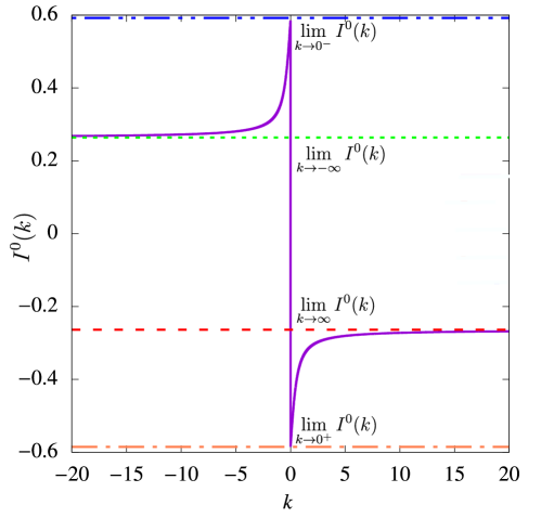
Figure 4: The integral $I^{0}(k)$ provided in Eq. (LABEL:indefinite_integral_rtp) plotted as a function of $k$ for fixed $s=1,~{}\gamma=1$ (solid purple curve). The integral has a discontinuity across the origin. The limiting forms $\lim_{k\rightarrow\infty}I^{0}(k),~{}lim_{k\rightarrow-\infty}I^{0}(k),~{}lim_{k\rightarrow 0^{+}}I^{0}(k)$ and  $lim_{k\rightarrow 0^{-}}I^{0}(k)$ are provided in Eqs. (118) and (119).

The indefinite integral $I^{0}(k)$ can be explicitly computed as

$$I^{0}(k) = \frac{1}{2s^{3/2}(s+2\gamma)\sqrt{-(2k+is)}}\times$$

$$\Biggl{[}\sqrt{(2k+is)(s+2\gamma)}\left(\tanh^{-1}\left(\frac{\sqrt{(2k+is)(s+2\gamma)}}{\sqrt{s(2k+i(s+4\gamma))}}\right)-\tanh^{-1}\left(\frac{\sqrt{(2k-is)(s+2\gamma)}}{\sqrt{s(2k-i(s+4\gamma))}}\right)\right)$$

$$+ \sqrt{(2k+is)(s+4\gamma)}\left(\tanh^{-1}\left(\frac{\sqrt{(2k-is)(s+4\gamma)}}{\sqrt{s(2k-i(s+4\gamma))}}\right)-\tanh^{-1}\left(\frac{\sqrt{(2k+is)(s+4\gamma)}}{\sqrt{s(2k+i(s+4\gamma))}}\right)\right)\Biggr{]}.$$

The function $I^{0}(k)$ has the typical behavior provided in Fig. 4. The definite integral in Eq. (114) can be computed simply as

$$\int_{0}^{\infty}\tilde{W}^{0}(z,s)dz = \frac{v}{2\pi}\Bigl{(}\lim_{k\rightarrow\infty}I^{0}(k)-\lim_{k\rightarrow 0^{+}}I^{0}(k)+\lim_{k\rightarrow 0^{-}}I^{0}(k)-\lim_{k\rightarrow-\infty}I^{0}(k)\Bigr{)}.$$ (117)

We need to extract the asymptotic behaviors of $I^{0}(k)$. These can be computed as

$$I^{0}(k)\xrightarrow[k\rightarrow\pm\infty]{}\ \mp\frac{\pi\left(\sqrt{\frac{s+4\gamma}{s+2\gamma}}-1\right)}{2s^{3/2}\sqrt{s+2\gamma}},$$ (118)

and

$$I^{0}(k)\xrightarrow[k\rightarrow 0^{\pm}]{}\ \mp\frac{\pi\sqrt{\frac{s+4\gamma}{s+2\gamma}}}{4s^{3/2}\sqrt{s+2\gamma}}.$$ (119)

Combining Eqs. (117), (118) and (119), we obtain the desired result in Eq. (34).

Let us next derive the expression provided in Eq. (48). One can use the Eqs. (45) and (111) and proceed exactly like the symmetric case. It is possible to show that

$$\int_{0}^{\infty}\tilde{W}^{\pm}(z,s)dz = \frac{v}{2\pi}\Bigl{(}\lim_{k\rightarrow\infty}I^{\pm}(k)-\lim_{k\rightarrow 0^{+}}I^{\pm}(k)+\lim_{k\rightarrow 0^{-}}I^{\pm}(k)-\lim_{k\rightarrow-\infty}I^{\pm}(k)\Bigr{)},$$ (120)

where $I^{\pm}(k)$ has the limiting behaviors

$$I^{+}(k)\xrightarrow[k\rightarrow\pm\infty]{}\ \mp\left(\frac{2\pi\gamma}{s^{3/2}(s+2\gamma)\sqrt{s+4\gamma}}-\frac{\pi+2K\left(-\frac{8\gamma(s+2\gamma)}{s^{2}}\right)}{4s(s+2\gamma)}\right),$$ (121)

$$I^{-}(k)\xrightarrow[k\rightarrow\pm\infty]{}\ \mp\left(\frac{2\pi\gamma}{s^{3/2}(s+2\gamma)\sqrt{s+4\gamma}}+\frac{\pi+2K\left(-\frac{8\gamma(s+2\gamma)}{s^{2}}\right)}{4s(s+2\gamma)}\right),$$ (122)

$$I^{+}(k)\xrightarrow[k\rightarrow 0^{\pm}]{}\ \mp\frac{\pi\left(\frac{1}{2\sqrt{s+2\gamma}}+\frac{\gamma}{(s+2\gamma)\sqrt{s+4\gamma}}\right)}{s^{3/2}},$$ (123)

and

$$I^{-}(k)\xrightarrow[k\rightarrow 0^{\pm}]{}\ \mp\frac{\pi\left(\frac{1}{2\sqrt{s+2\gamma}}+\frac{\gamma}{(s+2\gamma)\sqrt{s+4\gamma}}\right)}{s^{3/2}}.$$ (124)

Combining Eqs. (120)-(124), we recover the result provided in Eq. (48).

References

- [1] T. Vicsek, A. Czirók, E. Ben-Jacob, I. Cohen and O. Shochet, Novel type of phase transition in a system of self-driven particles, Physical Review Letters 75(6), 1226 (1995), 10.1103/PhysRevLett.75.1226.
- [2] A. Czirók, A.-L. Barabási and T. Vicsek, Collective motion of self-propelled particles: Kinetic phase transition in one dimension, Physical Review Letters 82(1), 209 (1999), 10.1103/PhysRevLett.82.209.
- [3] J. Tailleur and M. Cates, Statistical mechanics of interacting run-and-tumble bacteria, Physical Review Letters 100(21), 218103 (2008), 10.1103/PhysRevLett.100.218103.
- [4] B. Lindner and E. Nicola, Diffusion in different models of active brownian motion, The European Physical Journal Special Topics 157(1), 43 (2008), 10.1140/epjst/e2008-00629-7.
- [5] A. Cavagna, A. Cimarelli, I. Giardina, G. Parisi, R. Santagati, F. Stefanini and M. Viale, Scale-free correlations in starling flocks, Proceedings of the National Academy of Sciences 107(26), 11865 (2010), 10.1073/pnas.1005766107.
- [6] M. E. Cates, Diffusive transport without detailed balance in motile bacteria: does microbiology need statistical physics?, Reports on Progress in Physics 75(4), 042601 (2012), 10.1088/0034-4885/75/4/042601.
- [7] S. Ramaswamy, The mechanics and statistics of active matter, Annual Review of Condensed Matter Physics 1(1), 323 (2010), 10.1146/annurev-conmatphys-070909-104101.
- [8] P. Romanczuk and U. Erdmann, Collective motion of active brownian particles in one dimension, The European Physical Journal Special Topics 187(1), 127 (2010), 10.1140/epjst/e2010-01277-0.
- [9] P. Romanczuk, M. Bär, W. Ebeling, B. Lindner and L. Schimansky-Geier, Active brownian particles-from individual to collective stochastic dynamics, The European Physical Journal Special Topics 202 (2012), 10.1140/epjst/e2012-01529-y.
- [10] K. Martens, L. Angelani, R. Di Leonardo and L. Bocquet, Probability distributions for the run-and-tumble bacterial dynamics: An analogy to the lorentz model, The European Physical Journal E 35(9), 1 (2012), 10.1140/epje/i2012-12084-y.
- [11] L. Angelani, R. Di Leonardo and M. Paoluzzi, First-passage time of run-and-tumble particles, The European Physical Journal E 37(7), 1 (2014), 10.1140/epje/i2014-14059-4.
- [12] M. R. Evans and S. N. Majumdar, Run and tumble particle under resetting: a renewal approach, Journal of Physics A: Mathematical and Theoretical 51(47), 475003 (2018), 10.1088/1751-8121/aae74e.
- [13] M. E. Cates and J. Tailleur, When are active brownian particles and run-and-tumble particles equivalent? consequences for motility-induced phase separation, Europhysics Letters 101(2), 20010 (2013), 10.1209/0295-5075/101/20010.
- [14] M. Kourbane-Houssene, C. Erignoux, T. Bodineau and J. Tailleur, Exact hydrodynamic description of active lattice gases, Physical Review Letters 120(26), 268003 (2018), 10.1103/PhysRevLett.120.268003.
- [15] C. Merrigan, K. Ramola, R. Chatterjee, N. Segall, Y. Shokef and B. Chakraborty, Arrested states in persistent active matter: Gelation without attraction, Physical Review Research 2(1), 013260 (2020), 10.1103/PhysRevResearch.2.013260.
- [16] C. F. Lee, Active particles under confinement: aggregation at the wall and gradient formation inside a channel, New Journal of Physics 15(5), 055007 (2013), 10.1088/1367-2630/15/5/055007.
- [17] K. Malakar, V. Jemseena, A. Kundu, K. V. Kumar, S. Sabhapandit, S. N. Majumdar, S. Redner and A. Dhar, Steady state, relaxation and first-passage properties of a run-and-tumble particle in one-dimension, Journal of Statistical Mechanics: Theory and Experiment 2018(4), 043215 (2018), 10.1088/1742-5468/aab84f.
- [18] F. Mori, P. Le Doussal, S. N. Majumdar and G. Schehr, Universal survival probability for a d-dimensional run-and-tumble particle, Physical Review Letters 124(9), 090603 (2020), 10.1103/PhysRevLett.124.090603.
- [19] F. Mori, P. Le Doussal, S. N. Majumdar and G. Schehr, Universal properties of a run-and-tumble particle in arbitrary dimension, Physical Review E 102(4), 042133 (2020), 10.1103/PhysRevE.102.042133.
- [20] S. Jose, D. Mandal, M. Barma and K. Ramola, Active random walks in one and two dimensions, Physical Review E 105(6), 064103 (2022), 10.1103/PhysRevE.105.064103.
- [21] S. Jose, First passage statistics of active random walks on one and two dimensional lattices, Journal of Statistical Mechanics: Theory and Experiment 2022(11), 113208 (2022), 10.1088/1742-5468/ac9bef.
- [22] I. Santra, U. Basu and S. Sabhapandit, Run-and-tumble particles in two dimensions: Marginal position distributions, Physical Review E 101(6), 062120 (2020), 10.1103/PhysRevE.101.062120.
- [23] F. Mori, P. Le Doussal, S. N. Majumdar and G. Schehr, Condensation transition in the late-time position of a run-and-tumble particle, Physical Review E 103(6), 062134 (2021), 10.1103/PhysRevE.103.062134.
- [24] D. S. Dean, S. N. Majumdar and H. Schawe, Position distribution in a generalized run-and-tumble process, Physical Review E 103(1), 012130 (2021), 10.1103/PhysRevE.103.012130.
- [25] S. Das, G. Gompper and R. G. Winkler, Confined active brownian particles: theoretical description of propulsion-induced accumulation, New Journal of Physics 20(1), 015001 (2018), 10.1088/1367-2630/aa9d4b.
- [26] F. J. Sevilla, A. V. Arzola and E. P. Cital, Stationary superstatistics distributions of trapped run-and-tumble particles, Physical Review E 99(1), 012145 (2019), 10.1103/PhysRevE.99.012145.
- [27] L. Caprini and U. M. B. Marconi, Active chiral particles under confinement: Surface currents and bulk accumulation phenomena, Soft matter 15(12), 2627 (2019), 10.1039/C8SM02492H.
- [28] B. De Bruyne, S. N. Majumdar and G. Schehr, Survival probability of a run-and-tumble particle in the presence of a drift, Journal of Statistical Mechanics: Theory and Experiment 2021(4), 043211 (2021), 10.1088/1742-5468/abf5d5.
- [29] T. Agranov, S. Ro, Y. Kafri and V. Lecomte, Exact fluctuating hydrodynamics of active lattice gases—typical fluctuations, Journal of Statistical Mechanics: Theory and Experiment 2021(8), 083208 (2021), 10.1088/1742-5468/ac1406.
- [30] T. Agranov, S. Ro, Y. Kafri and V. Lecomte, Macroscopic fluctuation theory and current fluctuations in active lattice gases, SciPost Physics 14(3), 045 (2023), 10.21468/SciPostPhys.14.3.045.
- [31] T. Agranov, M. E. Cates and R. L. Jack, Entropy production and its large deviations in an active lattice gas, Journal of Statistical Mechanics: Theory and Experiment 2022(12), 123201 (2022), 10.1088/1742-5468/aca0eb.
- [32] S. Jose, R. Dandekar and K. Ramola, Current fluctuations in an interacting active lattice gas, Journal of Statistical Mechanics: Theory and Experiment 2023, 083208 (2023), 10.1088/1742-5468/aceb53.
- [33] B. Derrida, B. Douçot and P.-E. Roche, Current fluctuations in the one-dimensional symmetric exclusion process with open boundaries, Journal of Statistical Physics 115, 717 (2004), 10.1023/B:JOSS.0000022379.95508.b2.
- [34] B. Derrida and A. Gerschenfeld, Current fluctuations of the one dimensional symmetric simple exclusion process with step initial condition, Journal of Statistical Physics 136(1), 1 (2009), 10.1007/s10955-009-9772-7.
- [35] B. Derrida and A. Gerschenfeld, Current fluctuations in one dimensional diffusive systems with a step initial density profile, Journal of Statistical Physics 137(5), 978 (2009), 10.1007/s10955-009-9830-1.
- [36] P. Krapivsky and B. Meerson, Fluctuations of current in nonstationary diffusive lattice gases, Physical Review E 86(3), 031106 (2012), 10.1103/PhysRevE.86.031106.
- [37] K. Mallick, H. Moriya and T. Sasamoto, Exact solution of the macroscopic fluctuation theory for the symmetric exclusion process, Physical Review Letters 129(4), 040601 (2022), 10.1103/PhysRevLett.129.040601.
- [38] R. Dandekar, P. Krapivsky and K. Mallick, Dynamical fluctuations in the riesz gas, Physical Review E 107, 044129 (2023), 10.1103/PhysRevE.107.044129.
- [39] D. S. Dean, S. N. Majumdar and G. Schehr, Effusion of stochastic processes on a line, Journal of Statistical Mechanics: Theory and Experiment 2023, 063208 (2023), 10.1088/1742-5468/acdac4.
- [40] T. Banerjee, S. N. Majumdar, A. Rosso and G. Schehr, Current fluctuations in noninteracting run-and-tumble particles in one dimension, Physical Review E 101(5), 052101 (2020), 10.1103/PhysRevE.101.052101.
- [41] S. Jose, A. Rosso and K. Ramola, Generalized disorder averages and current fluctuations in run and tumble particles (2023), https://doi.org/10.48550/arXiv.2306.13613.
- [42] T. Chakraborty and P. Pradhan, Time-dependent properties of run-and-tumble particles. ii.: Current fluctuations (2023), https://doi.org/10.48550/arXiv.2309.02896.
- [43] T. Banerjee, R. L. Jack and M. E. Cates, Role of initial conditions in diffusive systems: compressibility, hyperuniformity and long-term memory, Physical Review E 106, L062101 (2022), 10.1103/PhysRevE.106.L062101.
- [44] N. Leibovich and E. Barkai, Everlasting effect of initial conditions on single-file diffusion, Physical Review E 88(3), 032107 (2013), 10.1103/PhysRevE.88.032107.