Can acoustic early dark energy still resolve the Hubble tension?

Abstract

In this paper, we re-assess the ability of the acoustic early dark energy (ADE) model to resolve the Hubble tension in light of the new Pantheon+ and S$H_{0}$ES data on the one hand, and the BOSS LRG and eBOSS QSO data, analysed under the effective field theory of large-scale structures (ETFofLSS) on the other hand. We find that the Pantheon+ data, which favor a larger $\Omega_{m}$ value than the Pantheon data, have a strong constraining power on the ADE model, while the EFTofLSS analysis of the BOSS and eBOSS data only slightly increases the constraints. We establish that the ADE model is now ruled out as a solution to the Hubble tension, with a remaining tension of $3.6\sigma$. In addition, we find that the axion-like early dark energy model performs better when confronted to the same datasets, with a residual tension of $2.5\sigma$. This work shows that the Pantheon+ data can have a decisive impact on models which aim to resolve the Hubble tension.

I Introduction

The $\Lambda$ cold dark matter ($\Lambda$CDM) model provides a remarkable description of a wide variety of data from the early universe – such as cosmic microwave background (CMB) or big bang nucleosynthesis (BBN) –, as well as observations of large scale structure (LSS) from the late universe – including the baryon acoustic oscillation (BAO) and the uncalibrated luminosity distance to supernovae of type Ia (SNIa). However, as the accuracy of cosmological observations has improved, the concordance cosmological model starts showing several experimental discrepancies. Among them, the Hubble tension refers to the inconsistency between local measurements of the current expansion rate of the Universe, quantified by the Hubble constant $H_{0}$, and the values inferred from early universe data assuming the $\Lambda$CDM model. More precisely, this tension is essentially driven by the Planck Collaboration’s observation of the cosmic microwave background (CMB), which predicts a value of $H_{0}=67.27\pm 0.60$ km/s/Mpc Aghanim et al. (2020a) within the $\Lambda$CDM model, and the value measured by the S$H_{0}$ES Collaboration using the Cepheid-calibrated cosmic distance ladder, whose latest measurement yields $H_{0}=73.04\pm 1.04$ km/s/Mpc Riess et al. (2021, 2022). The disagreement between these observations results in a $\sim 5\sigma$ tension. Experimental efforts are underway to establish whether this discrepancy can be caused by systematic effects (see, e.g., Dainotti et al. (2021, 2022); Mortsell et al. (2022a, b); Follin and Knox (2018); Brout and Scolnic (2021)), but no definitive explanation has yet been found. This tension could therefore be indicative of new physics, most likely located in the pre-recombination era, which involves a reduction in the sound horizon before recombination Bernal et al. (2016); Aylor et al. (2019); Knox and Millea (2020); Camarena and Marra (2021); Efstathiou (2021); Schöneberg et al. (2021). Early dark energy (EDE) models are capable of producing such an effect by increasing the total energy density of the Universe before recombination with the addition of a scalar field Karwal and Kamionkowski (2016); Poulin et al. (2019); Smith et al. (2020); Niedermann and Sloth (2019, 2020); Ye and Piao (2020); Agrawal et al. (2019); Berghaus and Karwal (2020); Braglia et al. (2020, 2021); Gonzalez et al. (2020) (for review of EDE models see Ref. Poulin et al. (2023), and for a review of models that could resolve the Hubble tension see Refs. Di Valentino et al. (2021); Schöneberg et al. (2021)). In the following, we consider the specific case of acoustic dark energy (ADE) developed in Refs. Lin et al. (2019, 2020).

In this paper, we reassess the constraints on the ADE model and its ability to resolve the Hubble tension, by successively evaluating the impact of the effective field theory (EFT) full-shape analysis applied to the BOSS LRG Alam et al. (2017) and eBOSS QSO Alam et al. (2021) data, and the impact of the Pantheon+ data Brout et al. (2022). On the one hand, we make use of developments of the one-loop prediction of the galaxy power spectrum in redshift space from the effective field theory of large-scale structures (EFTofLSS) Baumann et al. (2012); Carrasco et al. (2012); Senatore and Zaldarriaga (2015); Senatore (2015); Senatore and Zaldarriaga (2014); Perko et al. (2016) applied to the BOSS D’Amico et al. (2020a) and eBOSS Simon et al. (2023a) data in order to constrain the ADE model. This novel theoretical framework has made it possible to determine the $\Lambda$CDM parameters at precision higher than that from conventional BAO and redshift space distortions analyses, and even comparable to that of CMB experiments. In addition, the EFTofLSS provides an important consistency test for the $\Lambda$CDM model and its underlying assumptions, while allowing one to derive competitive constraints on models beyond $\Lambda$CDM (see, e.g., Refs. D’Amico et al. (2020a); Colas et al. (2020); D’Amico et al. (2020b, c); Simon et al. (2022, 2023b); Chen et al. (2022); Zhang et al. (2022); Philcox and Ivanov (2022); Kumar et al. (2022); Nunes et al. (2022); Laguë et al. (2021); Smith et al. (2022); Simon et al. (2023a); Moretti et al. (2023); Rubira et al. (2023); Schöneberg et al. (2023); Holm et al. (2023)). The study of the EFTofLSS impact on the ADE constraints is similar to what was carried out for the axion-like EDE in Ref. Simon et al. (2023c), which showed that this latter model leaves signatures in the galaxy power spectrum on large scales that can be probed by the BOSS data. On the other hand, we update the constraints on the ADE model by considering the Pantheon+ data from Ref. Brout et al. (2022). It has already been shown in Ref. Simon et al. (2023c) that the combination of the Pantheon+ data with a S$H_{0}$ES prior provides better constraints on the axion-like EDE model than the equivalent analysis including Pantheon data. This can be interpreted as a consequence of the fact that the Pantheon+ data prefers a value of $\Omega_{m}=0.334\pm 0.018$ which is higher than that of the Pantheon data. Together with the measured value of $H_{0}=100\cdot h$ km/s/Mpc by S$H_{0}$ES, it leads to an increased value of $\omega_{\rm cdm}=\Omega_{\rm cdm}\cdot h^{2}$, which cannot be fully compensated by the presence of EDE, therefore degrading slightly the fit to CMB data.

In Sec. II, we provide a review of the ADE and axion-like EDE models, as well as a description of the analysis method and the datasets to which these models will be subjected. In Sec. III, we present the constraints of the ADE model and compare them to the axion-like EDE case, while in Sec. IV we consider some additional variations of the model under study.

II The model and the data

II.1 Review of the ADE model

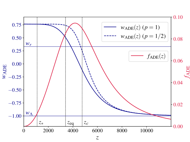
Figure 1: Evolution of the ADE equation of state parameter, $w_{\rm ADE}$, as well as the ADE fractional energy density, $f_{\rm ADE}(z_{c})$, as a function of the cosmological redshift $z$. To perform this plot, we use the best-fit values of the BAO/$f\sigma_{8}$ + Pan + $M_{b}$ analysis (see Tab. 1). For the ADE equation of state parameter, we set $p=1$, which corresponds to our baseline setup, and $p=1/2$, which corresponds to the setup of Ref. Lin et al. (2019). The horizontal lines correspond to the radiation and dark energy equation of state parameters, $w_{r}$ and $w_{\Lambda}$, respectively, while the dashed vertical lines correspond to the redshift of recombination $z_{*}$, the redshift of the matter-radiation equality $z_{\rm eq}$, and the ADE critical redshift $z_{c}$.

In this paper, we focus on the acoustic dark energy (ADE) model proposed in Ref. Lin et al. (2019) (see Ref. Poulin et al. (2023) for a general introduction). In this model, the ADE equation of state parameter, $w_{\rm ADE}(a)=P_{\rm ADE}(a)/\rho_{\rm ADE}(a)$, is modelled as

$$w_{\rm ADE}(a)=\frac{1+w_{f}}{\left[1+(a_{c}/a)^{3(1+w_{f})/p}\right]^{p}}-1\,.$$ (1)

In Fig. 1, we plot the evolution of $w_{\rm ADE}$ as a function of the cosmological redshift $z$. This figure clearly illustrates that in this model the critical redshift $z_{c}=(a_{0}-a_{c})/a_{c}$ sets a transition in the ADE equation of state from $w_{\rm ADE}\to-1$, when $z\gg z_{c}$, to $w_{\rm ADE}\to w_{f}$, when $z\ll z_{c}$. Therefore, this parametrization allows the ADE component to behave in a similar way to dark energy before the critical redshift (exactly like the axion-like EDE model), while it allows the late-time value of the ADE equation of state to be set thanks to the parameter $w_{f}$. As shown in Fig. 1, the rapidity of this transition is controlled by the parameter $p$, which is set at $p=1$ for our baseline model, corresponding to the modelling of the time averaged background equation of state of the axion-like EDE model Poulin et al. (2018). Similarly to the axion-like EDE case where $w_{\rm EDE}(z\ll z_{c})=1/2$ (see bellow), the ADE dilutes faster than the radiation (i.e., $w_{f}>w_{r}$) below the critical redshift, in order to suppress the contribution of this component to the total budget of the Universe at the moment of the CMB.

Let us note that the parametrization of Eq. (1) can be achieved in the K-essence class of dark energy models. In particular, the dark component is here a perfect fluid represented by a minimally-coupled scalar field $\phi$ with a general kinetic term Armendariz-Picon et al. (2001). For the specific case of a constant sound speed $c_{s}^{2}$, the Lagrangian density is written as Gordon and Hu (2004):

$$P(X,\phi)=\bigg{(}\frac{X}{A}\bigg{)}^{\frac{1-c_{s}^{2}}{2c_{s}^{2}}}X-V(\phi)\,,$$ (2)

where $X=-\nabla^{2}\phi/2$ and $A$ is a constant density scale Lin et al. (2019). In this category of models, $w_{\rm ADE}\to c_{s}^{2}$ if the kinetic term dominates, whereas $w_{\rm ADE}\to-1$ if the potential $V(\phi)$ dominates. The main advantage of the ADE model over the axion-like EDE model is that the former provides a general class of exact solutions, while the latter requires a specific set of initial conditions to achieve a similar phenomenology Lin et al. (2019).

Since the ADE equation of state parameter changes over time, the conservation equation gives

$$\rho_{\rm ADE}(a)=\rho_{\rm ADE,0}e^{3\int_{a}^{1}[1+w_{\rm ADE}(a^{\prime})]da^{\prime}/a^{\prime}}\,,$$ (3)

which allows us to define the ADE fractional energy density as

$$f_{\rm ADE}(a)=\frac{\rho_{\rm ADE}(a)}{\rho_{\rm tot}(a)}\,.$$ (4)

In Fig. 1, we also plot the evolution of $f_{\rm ADE}$ as a function of the cosmological redshift $z$. We notice that this parameter is maximal around the ADE equation of state transition, sets by the critical redshift $z_{c}$, namely when $f_{\rm ADE}(z\sim z_{c})$. Then, this parameter becomes subdominant at the time of recombination, with $f_{\rm ADE}(z_{*})\sim 1\%$.

Finally, the ADE model we are considering is described by the three following parameters

$$\{z_{c},\,f_{\rm ADE}(z_{c}),\,w_{f}\}\,.$$ (5)

Ref. Lin et al. (2019) also considers the variation of a fourth parameter that determines the behavior of the ADE perturbations, namely their rest frame sound speed $c_{s}^{2}(k,a)$. Unlike the standard axion-like EDE model (see bellow), we assume for this model the scale independence of this parameter, i.e., $c_{s}^{2}(k,a)=c_{s}^{2}(a)$, which is equivalent to assuming a perfect fluid with a linear dispersion relation. In addition, because of the sharp transition of the $w_{\rm ADE}$ parameter, the impact of the ADE component on the perturbed universe is localised in time, which implies that we can approximate this parameter as a constant. Thus, Ref. Lin et al. (2019) varies this parameter to its critical redshift value, namely $c_{s}^{2}=c_{s}^{2}(a=a_{c})$, in addition to the three other parameters listed above. In our baseline model, we consider that $c_{s}^{2}=w_{f}$, insofar as it has been shown to be a good approximation near the best-fit Lin et al. (2019). However, in Sec. IV, we consider two model variations of our baseline model: (i) the $c_{s}^{2}$ADE model, where we free these two parameters independently, and (ii) the cADE model, where we set $c_{s}^{2}=w_{f}=1$. Let us note that it exists a second difference between Refs. Lin et al. (2019, 2020) and our baseline analysis, since these references set $p=1/2$, which leads to a sharper transitions than ours (with $p=1$), as shown in Fig. 1. However, the impact of this parameter on cosmological results is very minor, and we have verified that we obtain the same results as Ref. Lin et al. (2020) with $p=1$.

II.2 Review of the axion-like EDE model

For comparison, we also consider the axion-like early dark energy (EDE) model Karwal and Kamionkowski (2016); Poulin et al. (2019); Smith et al. (2020), which corresponds to an extension of the $\Lambda$CDM model, where the existence of an additional subdominant oscillating scalar field $\phi$ is considered. The EDE field dynamics is described by the Klein-Gordon equation of motion (at the homogeneous level),

$$\ddot{\phi}+3H\dot{\phi}+V_{n,\phi}(\phi)=0\,,$$ (6)

where $V_{n}(\phi)$ is a modified axion-like potential defined as

$$V_{n}(\phi)=m^{2}f^{2}\left[1-\cos(\phi/f)\right]^{n}.$$ (7)

$f$ and $m$ correspond to the decay constant and the effective mass of the scalar field, respectively, while the parameter $n$ controls the rate of dilution after the field becomes dynamical. In the following, we will use the redefined field quantity $\Theta=\phi/f$ for convenience, such that $-\pi\leq\Theta\leq+\pi$. At early times, when $H\gg m$, the scalar field $\phi$ is frozen at its initial value since the Hubble friction prevails, which implies that the EDE behaves like a form of dark energy and that its contribution to the total energy density increases relative to the other components. When the Hubble parameter drops below a critical value ($H\sim m$), the field starts evolving toward the minimum of the potential and becomes dynamical. The EDE contribution to the total budget of the Universe is maximum around a critical redshift $z_{c}$, after which the energy density starts to dilute with an equation of state parameter $w_{\rm EDE}(a)$ approximated by Turner (1983); Poulin et al. (2018):

$$w_{\rm EDE}=\left\{\begin{array}[]{ll}-1&\text{if}\ z>z_{c},\\ \frac{n-1}{n+1}&\text{if}\ z<z_{c}.\end{array}\right.$$ (8)

In the following, we will fix $n=3$ as it was found that the data are relatively insensitive to this parameter provided $2\lesssim n\lesssim 5$ Smith et al. (2020), implying that in this specific model $w_{\rm EDE}(z\ll z_{c})=1/2$. Instead of the theory parameters $f$ and $m$, we make use of $z_{c}$ and $f_{\rm EDE}(z_{c})$, determined through a shooting method Smith et al. (2020). We also include the initial field value $\Theta_{i}$ as a free parameter, whose main role once $f_{\rm EDE}(z_{c})$ and $z_{c}$ are fixed is to set the dynamics of perturbations right around $z_{c}$, through the EDE sound speed $c_{s}^{2}$. Finally, the axion-like EDE model is described by the three following parameters:

$$\{z_{c},\,f_{\rm EDE}(z_{c}),\,\Theta_{i}\}\,.$$ (9)

Let us note that the axion-like EDE sound speed $c_{s}^{2}(a,k)=\delta P_{\rm EDE}(k,a)/\delta\rho_{\rm EDE}(k,a)$ is scale- and time-dependent, and is entirely determined by the three EDE parameters specified above. In the fluid approximation, one can estimate the $a$ and $k$ dependencies of this parameter as Poulin et al. (2018, 2019):

$$c^{2}_{s}(a,k)=\begin{cases}1\,,&a\leq a_{c},\\ \dfrac{2a^{2}(n-1)\varpi^{2}(a)+k^{2}}{2a^{2}(n+1)\varpi^{2}(a)+k^{2}}\,,&a>a_{c}\,,\end{cases}$$ (10)

where $\varpi$ corresponds to the angular frequency of the oscillating background field, which has a time dependency fixed by $z_{c}$, $n$ and $\Theta_{i}$ (see Ref. Poulin et al. (2018)). Let us note however that the axion-like EDE model we consider in this paper does not rely on this fluid approximation, and instead solves the exact (linearized) Klein-Gordon equation, which is expressed in synchronous gauge as Ma and Bertschinger (1995):

$$\delta\phi^{\prime\prime}_{k}+2H\delta\phi_{k}^{\prime}+\left[k^{2}+a^{2}V_{n,\phi\phi}\right]\delta\phi_{k}=-h^{\prime}\phi^{\prime}/2\,,$$ (11)

where the prime denotes derivatives with respect to conformal time.

II.3 Data and analysis methods

We perform Monte Carlo Markov Chain (MCMC) analyses, confronting the ADE model with recent cosmological observations. To do so, we make use of the Metropolis-Hastings algorithm from MontePython-v3 code Brinckmann and Lesgourgues (2018); Audren et al. (2013) interfaced with our modified CLASS Lesgourgues (2011); Blas et al. (2011) version. In this paper, we perform various analyses from a combination of the following datasets:

• Planck: The low-$\ell$ CMB temperature and polarization auto-correlations (TT, EE), and the high-$\ell$ TT, TE, EE data Aghanim et al. (2020b), as well as the gravitational lensing potential reconstruction from Planck 2018 Aghanim et al. (2020c).

• ext-BAO: The low-$z$ BAO data gathered from 6dFGS at $z=0.106$ Beutler et al. (2011), SDSS DR7 at $z=0.15$ Ross et al. (2015).

• BOSS BAO/$f\sigma_{8}$: BAO measurements, cross-correlated with the redshift space distortion measurements, from the CMASS and LOWZ galaxy samples of BOSS DR12 LRG at $z=0.38$, 0.51, and 0.61 Alam et al. (2017).

• eBOSS BAO/$f\sigma_{8}$: BAO measurements, cross-correlated with the redshift space distortion measurements, from the CMASS and LOWZ quasar samples of eBOSS DR16 QSO at $z=1.48$ Alam et al. (2021).

• EFTofBOSS: The EFTofLSS analysis of BOSS DR12 LRG, cross-correlated with the reconstructed BAO parameters Gil-Marín et al. (2016). The SDSS-III BOSS DR12 galaxy sample data and covariances are described in Alam et al. (2017); Kitaura et al. (2016). The measurements, obtained in Zhang et al. (2022), are from BOSS catalogs DR12 (v5) combined CMASS-LOWZ Reid et al. (2016), and are divided in redshift bins LOWZ, $0.2<z<0.43\ (z_{\rm eff}=0.32)$, and CMASS, $0.43<z<0.7\ (z_{\rm eff}=0.57)$, with north and south galactic skies for each, respectively denoted NGC and SGC. From these data we use the monopole and quadrupole moments of the galaxy power spectrum. The theory prediction and likelihood for the full-modeling information are made available through PyBird D’Amico et al. (2020b).

• EFTofeBOSS: The EFTofLSS analysis Simon et al. (2023a) of eBOSS DR16 QSOs Alam et al. (2021). The QSO catalogs are described in Ross et al. (2020) and the covariances are built from the EZ-mocks described in Chuang et al. (2015). There are about 343 708 quasars selected in the redshif range $0.8<z<2.2$, with $z_{\rm eff}=1.52$, divided into two skies, NGC and SGC Beutler and McDonald (2021); Hou et al. (2020). From these data we use the monopole and quadrupole moments of the galaxy power spectrum. The theory prediction and likelihood for the full-modeling information are made available through PyBird.

• Pantheon: The Pantheon catalog of uncalibrated luminosity distance of type Ia supernovae (SNeIa) in the range ${0.01<z<2.3}$ Scolnic et al. (2018).

• Pantheon+: The newer Pantheon+ catalog of uncalibrated luminosity distance of type Ia supernovae (SNeIa) in the range ${0.001<z<2.26}$ Brout et al. (2022).

• Pantheon+/S$\bm{H_{0}}$ES: The Pantheon+ catalog cross-correlated with the absolute calibration of the SNeIa from S$H_{0}$ES Riess et al. (2021).

• $\bm{{M_{b}}}$: Gaussian prior from the most up-to-date late-time measurement of the absolute calibration of the SNeIa from S$H_{0}$ES, $M_{b}=-19.253\pm 0.027$ Riess et al. (2021), corresponding to $H_{0}=(73.04\pm 1.04)$ km/s/Mpc.

We choose Planck + ext-BAO + BOSS BAO/$f\sigma_{8}$ + eBOSS BAO/$f\sigma_{8}$ + Pantheon (optionally with the $M_{b}$ prior) as our baseline analysis, called, for the sake of simplicity, “BAO/$f\sigma_{8}$ + Pan.” In order to assess the impact of the EFT full-shape analysis of the BOSS and eBOSS data on the ADE resolution of the Hubble tension, we compare the baseline analysis with an equivalent analysis that includes the EFTofBOSS and EFTofeBOSS likelihoods instead of the BOSS and eBOSS BAO/$f\sigma_{8}$ likelihoods. This analysis is called “EFT + Pan.” Finally, in order to gauge the influence of the new Pantheon data, we replace the Pantheon likelihood with the Pantheon+ likelihood. This analysis, referred to as “EFT + PanPlus,” is compared with the aforementioned EFTofLSS analysis. In App. A, we show explicitly that the addition of the $M_{b}$ prior on top of the Pantheon+ likelihood is equivalent to the use of the full “Pantheon+/S$H_{0}$ES” likelihood as provided in Ref. Riess et al. (2021).

For all runs performed, we impose large flat priors on $\{\omega_{b},\omega_{\rm cdm},H_{0},A_{s},n_{s},\tau_{\rm reio}\}$, which correspond, respectively, to the dimensionless baryon energy density, the dimensionless cold dark matter energy density, the Hubble parameter today, the variance of curvature perturbations centered around the pivot scale $k_{p}=0.05$ Mpc^-1 (according to the Planck convention), the scalar spectral index, and the reionization optical depth. Regarding the free parameters of the ADE model, we impose logarithmic flat priors on $z_{c}$, and flat priors on $f_{\rm ADE}(z_{c})$ and $w_{\rm ADE}$,

$$3\leq\log_{10}(z_{c})\leq 4.5\,,$$

$$0\leq f_{\rm ADE}(z_{c})\leq 0.2\,,$$

$$0\leq w_{f}\leq 3.6\,.$$

Note that we have verified that a wider prior on $w_{f}$ does not impact our results. When we compare the ADE model with the axion-like EDE model, we use the following priors for the latter:

$$3\leq\log_{10}(z_{c})\leq 4\,,$$

$$0\leq f_{\rm EDE}(z_{c})\leq 0.5\,,$$

$$0\leq\Theta_{i}\leq\pi\,.$$

In this paper, we use Planck conventions for the treatment of neutrinos, that is, we include two massless and one massive species with $m_{\nu}=0.06$ eV Aghanim et al. (2020a). In addition, we use Hmcode Mead et al. (2020) to estimate the non-linear matter clustering solely for the purpose of the CMB lensing. We define our MCMC chains to be converged when the Gelman-Rubin criterion $R-1<0.05$. Finally, we extract the best-fit parameters from the procedure highlighted in the appendix of Ref. Schöneberg et al. (2021), and we produce our figures thanks to GetDist Lewis (2019).

In this paper, we compare the models with each other using two main metrics. Firstly, in order to assess the ability of an extended model $\mathcal{M}$ to fit all the cosmological data, we compute the Akaike Information Criterion (AIC) of this model relative to that of the $\Lambda$CDM. This metric is defined as follows

$$\Delta{\rm AIC}=\chi^{2}_{\rm min,\,\mathcal{M}}-\chi^{2}_{\rm min,\,\Lambda CDM}+2\cdot(M_{\mathcal{M}}-M_{\Lambda\rm CDM})\,,$$ (12)

where $\mathcal{M}\in\{{\rm ADE,\,EDE,\,}c_{s}^{2}{\rm ADE,\,cADE}\}$, and where $N_{\mathcal{M}}$ stands for the number of free parameters of the model. This metric enables us to determine whether the fit within a particular model $\mathcal{M}$ significantly improves that of $\Lambda$CDM by penalizing models with a larger number of degrees of freedom. Secondly, in order to gauge the ability of the extended model $\mathcal{M}$ to solve the Hubble tension for a given combination of data $\mathcal{D}$ (which does not include the $M_{b}$ prior), we also compute the residual Hubble tension thanks to the difference in maximum a posterior (DMAP) Raveri and Hu (2019), determined by

$$Q_{\rm DMAP}=\sqrt{\chi^{2}_{\rm min,\,\mathcal{M}}(\mathcal{D}+M_{b})-\chi^{2}_{\rm min,\,\mathcal{M}}(\mathcal{D})}\,.$$ (13)

This metric allows us to determine how does the addition of the $M_{b}$ prior to the dataset $\mathcal{D}$ impact the fit within a particular model $\mathcal{M}$. Ref. Schöneberg et al. (2021) asserts that a model is a good candidate for solving the Hubble tension if it meets these two conditions: $\Delta AIC<-6.91$ and $Q_{\rm DMAP}<3\sigma$.

III Cosmological results

	BAO/$f\sigma_{8}$ + Pan		EFT + Pan		EFT + PanPlus
$M_{b}$ prior?	no	yes	no	yes	no	yes
$f_{\rm ADE}(z_{c})$	$<0.060(0.034)$	$0.081(0.090)\pm 0.018$	$<0.049(0.010)$	$0.068(0.076)\pm 0.019$	$<0.036(0.011)$	$0.073(0.082)\pm 0.020$
$\log_{10}(z_{c})$	$unconst.(3.748)$	$3.655(3.677)\pm 0.093$	$unconst.(3.713)$	$3.676(3.686)^{+0.095}_{-0.120}$	$unconst.(3.957)$	$3.692(3.724)^{+0.098}_{-0.120}$
$w_{f}$	$>0.49(0.69)$	$0.79(0.76)^{+0.10}_{-0.12}$	$>0.59(0.70)$	$0.78(0.75)^{+0.11}_{-0.13}$	$>0.61(0.57)$	$0.76(0.73)\pm 0.13$
$H_{0}$	$68.44(69.04)^{+0.47}_{-0.93}$	$71.24(71.49)\pm 0.68$	$68.16(68.26)^{+0.41}_{-0.53}$	$71.01(71.31)\pm 0.73$	$68.03(68.16)^{+0.43}_{-0.53}$	$71.13(71.29)\pm 0.73$
$\omega_{\rm cdm}$	$0.1212(0.1239)^{+0.0012}_{-0.0030}$	$0.1291(0.1305)\pm 0.0027$	$0.1196(0.1202)^{+0.0009}_{-0.0015}$	$0.1267(0.1280)\pm 0.0027$	$0.1201(0.1211)^{+0.0011}_{-0.0015}$	$0.1278(0.1294)\pm 0.0028$
$10^{2}\omega_{b}$	$2.259(2.269)^{+0.016}_{-0.023}$	$2.304(2.309)\pm 0.021$	$2.254(2.252)^{+0.014}_{-0.017}$	$2.303(2.306)\pm 0.022$	$2.250(2.258)\pm 0.018$	$2.306(2.311)\pm 0.022$
$10^{9}A_{s}$	$2.123(2.119)\pm 0.030$	$2.159(2.152)\pm 0.031$	$2.111(2.111)\pm 0.030$	$2.148(2.151)^{+0.028}_{-0.032}$	$2.111(2.116)^{+0.028}_{-0.036}$	$2.151(2.150)^{+0.028}_{-0.033}$
$n_{s}$	$0.9711(0.9748)^{+0.0041}_{-0.0074}$	$0.9900(0.9925)\pm 0.0061$	$0.9684(0.9686)^{+0.0040}_{-0.0048}$	$0.9878(0.9904)\pm 0.0060$	$0.9679(0.9697)^{+0.0038}_{-0.0047}$	$0.9890(0.9906)\pm 0.0063$
$\tau_{\rm reio}$	$0.0583(0.0540)^{+0.0063}_{-0.0075}$	$0.0588(0.0561)^{+0.0066}_{-0.0077}$	$0.0572(0.0573)\pm 0.0070$	$0.0590(0.0584)^{+0.0067}_{-0.0077}$	$0.0570(0.0574)\pm 0.0072$	$0.0585(0.0573)^{+0.0065}_{-0.0077}$
$S_{8}$	$0.828(0.834)^{+0.011}_{-0.013}$	$0.843(0.846)\pm 0.013$	$0.820(0.823)\pm 0.010$	$0.832(0.835)\pm 0.012$	$0.825(0.830)^{+0.010}_{-0.011}$	$0.836(0.842)\pm 0.013$
$\Omega_{m}$	$0.3083(0.3089)\pm 0.0054$	$0.3011(0.3018)\pm 0.0050$	$0.3074(0.3078)\pm 0.0050$	$0.2983(0.2983)\pm 0.0047$	$0.3096(0.3107)^{+0.0047}_{-0.0053}$	$0.2994(0.3014)\pm 0.0047$
$\Delta\chi^{2}_{\rm min}$	-3.9	-28.3	-1.4	-24.9	-1.3	-27.8
$\Delta$AIC	+2.1	-22.3	+4.6	-18.9	+4.7	-21.8
$Q_{\rm DMAP}$	2.6$\sigma$		2.9$\sigma$		3.6$\sigma$
$Q_{\rm DMAP}(\rm EDE)$	1.5$\sigma$		2.4$\sigma$		2.5$\sigma$
$Q_{\rm DMAP}(\Lambda\rm CDM)$	5.6$\sigma$		5.6$\sigma$		6.3$\sigma$

Table 1: Mean (best-fit) $\pm 1\sigma$ (or $2\sigma$ for one-sided bounds) of reconstructed parameters in the ADE model confronted to various datasets. All datasets include Planck + ext-BAO data, while we consider either the BAO/$f\sigma_{8}$ information or the EFT full-shape analysis for the BOSS and eBOSS data, and we consider either the Pantheon data or the Pantheon+ data (with and without the $M_{b}$ prior). We also display for all datasets the $\Delta\chi^{2}_{\rm min}$ with respect to $\Lambda$CDM, the associated $\Delta$AIC, as well as the $Q_{\rm DMAP}$. Finally, $Q_{\rm DMAP}(\Lambda\rm CDM)$ and $Q_{\rm DMAP}(\rm EDE)$ corresponds the $Q_{\rm DMAP}$ of the $\Lambda$CDM and axion-like EDE models for the equivalent datasets.

In this section, we discuss the cosmological constraints of the ADE model and its ability to solve the Hubble tension by successively evaluating the impact of the EFT full-shape analysis of the BOSS and eBOSS data (compared with the standard BAO/$f\sigma_{8}$ analysis) and the impact of the new Pantheon data (compared with the equivalent older data) on this model. The cosmological constraints are shown in Tab. 1, while the $\chi^{2}_{\rm min}$ values associated with each likelihood are presented in Tab. 3 of App. B. In Tab. 1, we also display the $\Delta\chi^{2}_{\rm min}$ and the associated $\Delta$AIC with respect to $\Lambda$CDM, as well as the $Q_{\rm DMAP}$ for several combinations of data.

Our baseline combination of data, denoted “BAO/$f\sigma_{8}$ + Pan,” refers to Planck + ext-BAO + BOSS BAO/$f\sigma_{8}$ + eBOSS BAO/$f\sigma_{8}$ + Pantheon, corresponding roughly to that used in Ref. Lin et al. (2020). For this analysis, combined with the $M_{b}$ prior, we find $f_{\rm ADE}(z_{c})=0.081\pm 0.018$ and $H_{0}=71.24\pm 0.68$ km/s/Mpc, leading to a residual Hubble tension of $Q_{\rm DMAP}=2.6\sigma$ and a preference over $\Lambda$CDM of $\Delta{\rm AIC}=-22.3$ (see Tab. 1). Note that with this combination of data, the ADE model satisfies both Ref. Schöneberg et al. (2021) conditions. We are now assessing how the EFTofLSS on the one hand, and the new data from Pantheon+ on the other hand, change these conclusions.

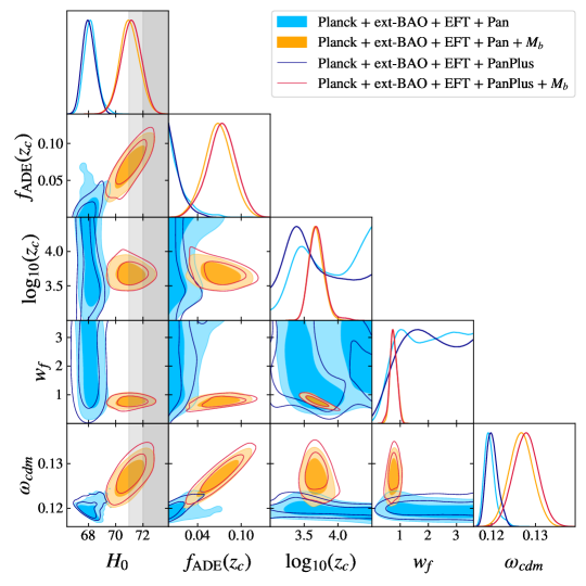
Figure 2: Top panel: 2D posterior distributions reconstructed from the BAO/$f\sigma_{8}$ + Pan dataset compared with the 2D posterior distributions reconstructed from the EFT + Pan dataset, either with or without the $M_{b}$ prior. Bottom panel: 2D posterior distributions reconstructed from the EFT + Pan dataset compared with the 2D posterior distributions reconstructed from the EFT + PanPlus dataset, either with or without the $M_{b}$ prior. The gray bands correspond to the $H_{0}$ constraint associated with the $M_{b}$ prior, $H_{0}=(73.04\pm 1.04)$ km/s/Mpc Riess et al. (2021).

III.1 Impact of the EFTofLSS analysis

In the top panel of Fig. 2, we show the reconstructed 2D posteriors of the ADE model for the analysis with the BOSS and eBOSS BAO/$f\sigma_{8}$ likelihoods (namely the BAO/$f\sigma_{8}$ + Pan analysis), as well as for the analysis with the EFTofBOSS and EFTofeBOSS likelihoods (namely the EFT + Pan analysis), either with or without the $M_{b}$ prior. To isolate the effect of the EFT full-shape analysis, we carry out these analyses using only the older Pantheon data.

For the analyses without the $M_{b}$ prior, the addition of the EFT likelihood has a non-negligible impact on the $f_{\rm ADE}(z_{c})$, $w_{f}$, and $H_{0}$ constraints. The upper bound of the ADE fractional energy density and the lower bound of $w_{f}$ are indeed both improved by $\sim 20\%$, while the standard deviation of $H_{0}$ is reduced by $\sim 35\%$.

When we consider the $M_{b}$ prior, EFTofBOSS and EFTofeBOSS do not improve the parameter constraints of this model over the BAO/$f\sigma_{8}$ information. However, these likelihoods shift $f_{\rm ADE}(z_{c})$ and $H_{0}$ towards smaller values of $0.7\sigma$ and $0.3\sigma$, respectively. The EFT full-shape analysis of the BOSS and eBOSS data therefore slightly reduces the ability of this model to resolve the Hubble tension, and the $Q_{\rm DMAP}$ changes from $2.6\sigma$ to $2.9\sigma$ when EFT likelihoods are considered (see Tab. 1). In particular, the $\chi^{2}_{\rm min}$ associated with the $M_{b}$ prior is degraded by $1.0$ compared to the BAO/$f\sigma_{8}$ analysis. In addition, the preference for this model over the $\Lambda$CDM model is slightly reduced, given that the $\Delta{\rm AIC}$ changes from $-22.3$ to $-18.9$ when the EFT likelihood is added (see Tab. 1). Note that at this point, the ADE model still satisfies both conditions of Ref. Schöneberg et al. (2021), even though $Q_{\rm DMAP}\sim 3\sigma$.

For the axion-like EDE case, we find for the equivalent analyses (see Tab. 3 of App. B) that the $Q_{\rm DMAP}$ changes from $1.5\sigma$ to $2.4\sigma$, and that the $\Delta{\rm AIC}$ changes from $-29.1$ to $-22.9$, when EFT likelihoods are added. The ADE model slightly better supports the addition of the EFT likelihood compared to the EDE model, insofar as the $Q_{\rm DMAP}$ and $\Delta{\rm AIC}$ are more stable (see Tab. 1). Unlike the $f\sigma_{8}$ information which assumes scale-independence, the EFT full-shape analysis allows to exploit the scale-dependence of the power spectrum. This may explain why the axion-like EDE model is better constrained by the EFTofLSS compared to the BAO/$f\sigma_{8}$ information, since this theory makes it possible to probe the scale-dependence of the EDE sound speed $c_{s}^{2}$. However, the EDE model remains a better model to solve the Hubble tension, with $Q_{\rm DMAP}=2.4\sigma$ for the EFT + Pan analysis, compared to $Q_{\rm DMAP}=2.9\sigma$ for the ADE model, and has a better fit to the data when the $M_{b}$ prior is added, with $\Delta{\rm AIC}=-22.9$, compared to $\Delta{\rm AIC}=-18.9$ for the ADE model. For a detailed discussion of the EFTofLSS impact on the EDE model in the framework of the BOSS data, please refer to Ref. Simon et al. (2023c).

III.2 Impact of the Pantheon+ data

Let’s now turn to the impact of the latest Pantheon data, namely the Pantheon+ data, on the ability of this model to resolve the Hubble tension. In the bottom panel of Fig. 2, we show the reconstructed 2D posteriors of the ADE model for the analyses with the old Pantheon data (i.e., the EFT + Pan analysis), as well as for the analyses with the updated data (i.e., the EFT + PanPlus analysis). To isolate the effect of the Pantheon+ data, we carry out these analyses using only the EFT full-shape analysis of the BOSS and eBOSS data.

The analysis with the Pantheon+ data, but without any S$H_{0}$ES prior, improves significantly the $95\%$ C.L. constraints on $f_{\rm ADE}(z_{c})$ by $\sim 30\%$. This implies that $H_{0}$ is shifted down by $0.2\sigma$ compared to the analysis with the old Pantheon data. Although the ADE model prefers a higher value of $\omega_{\rm cdm}$ than $\Lambda$CDM (because ADE slows down the evolution of the growing modes), the larger $\Omega_{m}$ favored by the Pantheon+ data ($\Omega_{m}=0.334\pm 0.018$ Brout et al. (2022)) leads to a large $\omega_{\rm cdm}=\Omega_{\rm cdm}\cdot h^{2}$ which is not sufficiently compensated for by ADE. Then, to offset the high value of $\Omega_{m}$, the current Hubble parameter decreases slightly, as well as $f_{\rm ADE}(z_{c})$, since the latter is positively correlated with $H_{0}$.

When the $M_{b}$ prior is included, non-zero contribution of ADE are favored. One may have expected that the tighter constraints from Pantheon+ may reduce the contribution of $f_{\rm ADE}$ and the value of $H_{0}$. These are in fact stable when compared to analyses with the older Pantheon data, with similar error bars between the EFT + Pan + $M_{b}$ and EFT + PanPlus + $M_{b}$ analyses. Thus, if we rely solely on the posterior distributions, we could argue that the Pantheon+ data do not change the conclusion about the ADE resolution of the Hubble tension. However, it turns out that the ADE model is not able to accommodate at the same time the large value of $H_{0}$ and $\Omega_{m}$ that are favored by the Pantheon+ data once they are calibrated with $M_{b}$. Indeed, the best-fit value $H_{0}=71.29$ km/s/Mpc is $1.7\sigma$ lower than the S$H_{0}$ES constraint [$H_{0}=(73.04\pm 1.04)$ km/s/Mpc], while the best-fit value $\Omega_{m}=0.3014$ is $1.8\sigma$ lower than the Pantheon+ constraint [$\Omega_{m}=0.334\pm 0.018$]. Therefore, the ADE model does not provide a good fit to the $M_{b}$ prior ($\chi^{2}_{M_{b}}=6.42$ as shown in Tab. 3 of App. B), while the fit to the Pantheon+ data is worsen (by +1.6) with the inclusion of the $M_{b}$ prior. These degradations of $\chi^{2}_{\rm min}$ imply that the $Q_{\rm DMAP}$ changes from $2.9\sigma$ ($5.6\sigma$ for $\Lambda$CDM) to $3.6\sigma$ ($6.3\sigma$ for $\Lambda$CDM) when we consider the Pantheon+ data (see Tab. 1), which severely limits the ability of this model to resolve the $H_{0}$ tension. One of the two criteria of Ref. Schöneberg et al. (2021), namely $Q_{\rm DMAP}<3\sigma$, is indeed no longer fulfilled. However, while the Pantheon+ data and the $M_{b}$ prior from Ref. Riess et al. (2021) seriously restrict the ability of the ADE model to resolve the Hubble tension, these data improve the preference for this model over $\Lambda$CDM, since the $\Delta{\rm AIC}$ changes from $-18.9$ to $-21.8$. We nevertheless caution over-interpreting this preference, given that the $Q_{\rm DMAP}$ indicates that combining these datasets is not statistically consistent.

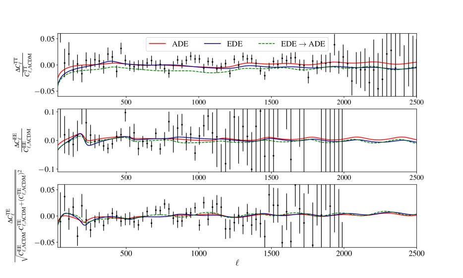
Figure 3: CMB power spectra residuals with respect to $\Lambda$CDM for the ADE (red) and axion-like EDE (black) models. All cosmological parameters of the $\Lambda$CDM, ADE, and axion-like EDE models have been set to their EFT + PanPlus best-fits, while the displayed data (nomalized to the $\Lambda$CDM best-fit) correspond to the Planck 2018 data Aghanim et al. (2020b). Finally, for the plot entitled “EDE $\to$ ADE,” we set the $\Lambda$CDM parameters to the axion-like EDE best-fit, while the $z_{c}$ and $w_{f}$ parameters are set to the ADE best-fit. The last ADE parameter, namely $f_{\rm ADE}(z_{c})=0.095$, is determined such that the values of $100\theta_{s}=1.042$ and $r_{s}=140.53$ Mpc are the same as for the EDE best-fit.

In the left panel of Fig. 4, we show the 2D posterior distributions of the axion-like EDE model reconstructed from the EFT + PanPlus + $M_{b}$ dataset, while the associated cosmological constraints are displayed in Tab. 2. For the axion-like EDE case, we find that the $Q_{\rm DMAP}$ changes from $2.4\sigma$ to $2.5\sigma$, and that the $\Delta{\rm AIC}$ changes from $-22.9$ to $-29.1$, between the old and the new Pantheon data analysis (see Tab. 3 of App. B for the individual $\chi^{2}_{\rm min}$). This model better supports these new data, since the $Q_{\rm DMAP}$ is stable (and especially the $\chi^{2}_{\rm min}$ of the S$H_{0}$ES prior), while the $\Delta{\rm AIC}$, as in the case of the ADE model, decreases significantly. Whereas with the addition of the EFT data we had a slight preference for EDE over ADE, with the Pantheon+ data the preference for this model becomes clearly apparent: in the axion-like EDE model, $H_{0}=71.67\pm 0.77$ km/s/Mpc with $Q_{\rm DMAP}=2.5\sigma$, while in the ADE model, $H_{0}=71.13\pm 0.73$ km/s/Mpc with $Q_{\rm DMAP}=3.6\sigma$. In addition, the axion-like EDE model provides a better overall fit than the ADE model, with $\Delta AIC({\rm EDE-ADE})=+7.3$. The two main contributions to this difference come from the Planck data (and in particular the high-$\ell$ TTTEEE likelihood), where $\Delta\chi^{2}({\rm EDE-ADE})=+3.7$, and from the S$H_{0}$ES prior, where $\Delta\chi^{2}({\rm EDE-ADE})=+2.7$. The axion-like EDE model is capable of better compensating the effect of large values of $H_{0}$ and $\Omega_{\rm m}$ (and therefore $\omega_{\rm cdm}$) on the CMB compared to the ADE model.

In order to understand why the axion-like EDE model performs better than ADE, we plot in Fig. 3 the CMB power spectra residuals with respect to the $\Lambda$CDM best-fit for these two models. On this figure, we also plot (in green dashed) the CMB power spectra residuals of the ADE model, where we set the $\Lambda$CDM parameters to the axion-like EDE best-fit, and the $z_{c}$ and $w_{f}$ parameters to the ADE best-fit. The last ADE parameter, namely $f_{\rm ADE}(z_{c})$, is dermined such that the values of the angular acoustic scale at recombination, $\theta_{*}$, and the comoving sound horizon at recombination, $r_{*}$, are the same as for the EDE best-fit. In other words, this plot would represent the best-fit of the ADE model if the latter could reduce the Hubble tension to the same level as the axion-like EDE model. In this figure, the main difference between the ADE and ADE $\to$ EDE plots stems from the suppression (particularly at low $\ell$) of the $C_{\ell}^{\rm TT}$ power spectrum for the EDE $\to$ ADE analysis. This suppression typically corresponds to the effect of a large value of $\omega_{\rm cdm}$ (and also $n_{s}$), showing that the ADE model is not able to compensate for a high value of $\Omega_{\rm cdm}h^{2}$ in the same way as the axion-like EDE model. This is explained by the fact that the EDE model allows the sound speed to decrease in the $k$ range associated with $\ell<500$, making it easier to compensate for the effect of increasing $\Omega_{\rm cdm}h^{2}$ in the low-$\ell$ TT power spectrum. Let us note that the effect of the increase in $\Omega_{\rm cdm}h^{2}$ is more significant for the modes that have re-entered the horizon at the time when $f_{\rm ADE}$ is decreasing, and therefore no longer significantly suppresses the evolution of the growing modes. In order to compensate for this effect, it is therefore helpful to decrease $c_{s}^{2}$ for $l<500$, insofar as a reduction in this parameter leads to an enhancement in the Weyl potential (see Ref. Lin et al. (2019)). Note that these results are compatible with Ref. Lin et al. (2019), but interestingly the limitation in the value of $\Omega_{\rm cdm}h^{2}$ does not arise from the CMB polarization as in that reference (which considered Planck 2015 data), but from the CMB temperature.

IV Model variations

	EDE	$c_{s}^{2}$ADE	cADE
$f_{\rm ADE/EDE}(z_{c})$	$0.116(0.128)^{+0.023}_{-0.021}$	$0.103(0.080)^{+0.028}_{-0.046}$	$0.079(0.087)\pm 0.019$
$\log_{10}(z_{c})$	$3.69(3.84)^{+0.20}_{-0.16}$	$3.61(3.73)^{+0.12}_{-0.10}$	$3.540(3.532)\pm 0.058$
$\Theta_{i}$	$2.77(2.88)^{+0.15}_{-0.072}$	–	–
$w_{f}$	–	$unconst.(0.71)$	–
$c_{s}^{2}$	–	$>0.701(0.72)$	–
$H_{0}$	$71.67(71.84)\pm 0.77$	$70.76(71.23)\pm 0.70$	$70.95(71.23)\pm 0.73$
$\omega_{\rm cdm}$	$0.1303(0.1309)\pm 0.0030$	$0.1257(0.1294)\pm 0.0024$	$0.1273(0.1286)\pm 0.0028$
$10^{2}\omega_{b}$	$2.294(2.312)\pm 0.024$	$2.304(2.310)\pm 0.020$	$2.305(2.308)\pm 0.021$
$10^{9}A_{s}$	$2.149(2.143)^{+0.027}_{-0.034}$	$2.152(2.150)^{+0.030}_{-0.036}$	$2.149(2.158)\pm 0.031$
$n_{s}$	$0.9898(0.9951)\pm 0.0061$	$0.9882(0.9902)\pm 0.0065$	$0.9849(0.9874)\pm 0.0057$
$\tau_{\rm reio}$	$0.0590(0.0590)^{+0.0063}_{-0.0079}$	$0.0592(0.0573)^{+0.0069}_{-0.0080}$	$0.0573(0.0583)^{+0.0066}_{-0.0078}$
$S_{8}$	$0.836(0.836)\pm 0.011$	$0.831(0.842)\pm 0.012$	$0.836(0.841)\pm 0.012$
$\Omega_{m}$	$0.2995(0.2997)\pm 0.0047$	$0.2985(0.3018)\pm 0.0049$	$0.3000(0.3001)\pm 0.0047$
$\Delta\chi^{2}_{\rm min}$	$-35.1$	$-27.9$	$-24.1$
$\Delta$AIC	$-29.1$	$-19.9$	$-20.1$
$Q_{\rm DMAP}$	$2.5\sigma$	$3.6\sigma$	$3.9\sigma$

Table 2: Mean (best-fit) $\pm 1\sigma$ (or $2\sigma$ for one-sided bounds) of reconstructed parameters in the EDE, $c_{s}^{2}$ADE, and cADE models confronted to the Planck + ext-BAO + EFT + PanPlus + $M_{b}$ dataset, i.e., the most up-to-date dataset. We also display for each model the $\Delta\chi^{2}_{\rm min}$ with respect to $\Lambda$CDM, the associated $\Delta$AIC, as well as the $Q_{\rm DMAP}$.

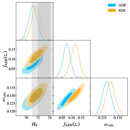
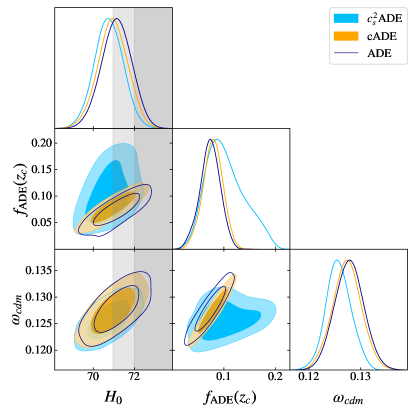
Figure 4: Left panel: 2D posterior distributions reconstructed from the Planck + ext-BAO + EFT + PanPlus + $M_{b}$ dataset, i.e., the most up-to-date dataset, for our baseline ADE model and the standard axion-like EDE model. Right panel: 2D posterior distributions reconstructed from the Planck + ext-BAO + EFT + PanPlus + $M_{b}$ dataset for the $c_{s}^{2}$ADE model (namely our baseline ADE model with the variation of $c_{s}^{2}$), the cADE model (namely our baseline ADE model with $c_{s}^{2}=w_{f}=1$), and our baseline ADE model. The gray bands correspond to the $H_{0}$ constraint associated with the $M_{b}$ prior, $H_{0}=(73.04\pm 1.04)$ km/s/Mpc Riess et al. (2021).

IV.1 Variation of $c_{s}^{2}$

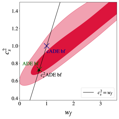
Figure 5: 2D posterior distribution of the $c_{s}^{2}-w_{f}$ plane reconstructed from the Planck + ext-BAO + EFT + PanPlus + $M_{b}$ dataset for the $c_{s}^{2}$ADE model. The solid line corresponds to $c_{s}^{2}=w_{f}$, while the blue and green crosses correspond respectively to the cADE model and the best-fit of our baseline ADE model. The black circle represents the best-fit of the $c_{s}^{2}$ADE model.

In the previous sections, we fixed $c_{s}^{2}(a_{c})=w_{f}$ instead of varying these two parameters independently. In the right panel of Fig. 4, we show the 2D posterior distributions reconstructed from the EFT + PanPlus + $M_{b}$ dataset for our baseline ADE model by relaxing this assumption, while in Tab. 2 we display the associated cosmological constraints. To do so, we have applied the prior of Refs. Lin et al. (2019, 2020) to $c_{s}^{2}$, namely

$$0\leq c_{s}^{2}\leq 1.5\,.$$

In the following, we simply call this extended model “$c_{s}^{2}$ADE,” for which we still consider that $p=1$. Interestingly, and in line with Ref. Lin et al. (2019), the assumption $c_{s}^{2}=w_{f}$ does not change our conclusions, especially regarding the Hubble tension: we obtain $Q_{\rm DMAP}=3.6\sigma$, which is similar to that of our baseline ADE model (see Tab. 3 of App. B for the $\chi^{2}$ values). In this specific case, we obtain $H_{0}=70.76\pm 0.70$ km/s/Mpc, which is $0.5\sigma$ lower than the $H_{0}$ value from our baseline ADE model. This is due to projection effects caused by the non-Gaussian posteriors of $c_{s}^{2}$ and $w_{f}$, and we notice that the best-fit value ($H_{0}=71.23$ km/s/Mpc) is very close to that of the ADE model. Thus, the relaxation of this hypothesis does not resolve the Hubble tension, while the $\Delta AIC$ worsens somewhat in this model because of the additional parameter ($\Delta AIC=-20.1$ instead of $-21.8$ for our baseline ADE model). In addition, as shown in Fig. 5, the best-fit point of the ADE model in the $c_{s}^{2}-w_{f}$ plane lies in the $68\%$ C.L. reconstructed from the $c_{s}^{2}$ADE model, and is very close to the best-fit point of this model. This implies that setting $c_{s}^{2}=w_{f}$ is a good approximation around the best-fit of the $c_{s}^{2}$ADE model.

IV.2 The cADE model

Refs. Lin et al. (2019) and Lin et al. (2020) showed that the special case where $c_{s}^{2}=w_{f}=1$ made it possible to solve the Hubble tension. In this particular model, called “cADE,” the ADE component is a canonical scalar which goes from a frozen phase ($w=-1$) to a kinetion phase ($w=1$) around matter-radiation equality. This model is particularly interesting because it allows the Hubble tension to be resolved with only two more parameters than the $\Lambda$CDM model [namely $f_{\rm ADE}(z_{c})$ and $\log_{10}(z_{c})$]. However, while in Ref. Lin et al. (2019) the case $c_{s}^{2}=w_{f}=1$ is within the $68\%$ C.L. of the $c_{s}^{2}$ and $w_{f}$ parameters (see Fig. 1 of this reference), one can see in Fig. 5 that this particular case is no longer located in the $1\sigma$ region. In the right panel of Fig. 4, we display the 2D posterior distributions of the cADE model reconstructed from the EFT + PanPlus + $M_{b}$ dataset, while in Tab. 2 we display the associated cosmological constraints. We can clearly see that this particular model is unable to resolve the Hubble tension with current data, since we obtain $H_{0}=70.95\pm 0.73$ km/s/Mpc and $f_{\rm ADE}(z_{c})=0.079\pm 0.019$, with a $Q_{\rm DMAP}=3.9\sigma$ (compared to $Q_{\rm DMAP}=3.6\sigma$ for our baseline ADE model).

V Conclusion

In this paper, we have updated the constraints on the acoustic dark energy model by first assessing the impact of the EFT full-shape analysis applied to the BOSS LRG and eBOSS QSO data, and secondly the impact of the latest Pantheon+ data.

• When we consider the full-shape analysis of the BOSS and eBOSS data, combined with Planck, ext-BAO measurements, Pantheon data from Scolnic et al. (2018), and S$H_{0}$ES data from Riess et al. (2021), we obtain $H_{0}=71.01\pm 0.73$ km/s/Mpc with a residual Hubble tension of $2.9\sigma$ (compared to $2.4\sigma$ for the axion-like EDE model and $5.6\sigma$ for the $\Lambda$CDM model).

• We have demonstrated that the EFTofLSS analysis slightly reduces the ability of this model to resolve the Hubble tension compared to the BAO/$f\sigma_{8}$ analysis, which has a residual tension of $2.6\sigma$ (with $H_{0}=71.24\pm 0.68$ km/s/Mpc).

• Although the axion-like EDE model remains a better solution to the Hubble tension after using the EFTofBOSS and EFTofeBOSS likelihoods, we have shown that the EFTofLSS analysis has a stronger impact on this model due to the scale dependence of the EDE sound speed probed by the EFT full-shape description of the LSS power spectra.

• Importantly, when we replace the Pantheon data with the Pantheons+ data from Brout et al. (2022), the ADE model no longer resolves the Hubble tension at a suitable level, leading to a $3.6\sigma$ residual tension (compared to $2.5\sigma$ for the EDE model and $6.3\sigma$ for the $\Lambda$CDM model).

• Whereas with the EFTofLSS analysis we had only a slight preference for EDE over ADE, with the new data from Pantheon+ and S$H_{0}$ES, the preference for this model becomes clearly apparent, due to the fact that axion-like EDE manages to compensate a higher $\Omega_{\rm cdm}h^{2}$ in Planck data thanks to the scale-dependence of the sound speed.
  

• Finally, we have verified that relaxing the assumption $c_{s}^{2}=w_{f}$ does not alter our conclusions, justifying this choice. In addition, for the cADE model (where $c_{s}^{2}=w_{f}=1$), we have obtained $H_{0}=70.95\pm 0.73$ km/s/Mpc with a $Q_{\rm DMAP}=3.9\sigma$, implying that one can no longer solve the Hubble tension with this constrained ADE model, contrary to previous results Lin et al. (2019, 2020).
  

In this paper, we have shown that the new data from Pantheon and S$H_{0}$ES, and to a lesser extent the EFTofLSS applied to the BOSS and eBOSS data, can have a decisive impact on models which aim to resolve the Hubble tension. We leave for future work the study of the impact on the Hubble tension of such an analysis applied to other early dark energy models, such as new early dark energy Niedermann and Sloth (2019, 2020), Rock ‘n’ Roll dark energy  Agrawal et al. (2019), or early modified gravity Braglia et al. (2021).

Appendix A $M_{b}$ prior

In this appendix, we show explicitly, thanks to Fig 6, that the addition of the $M_{b}$ prior Riess et al. (2021) on top of the Pantheon+ likelihood is equivalent to the use of the full Pantheon+/S$H_{0}$ES likelihood as provided in Ref. Riess et al. (2021). Since the constraints are similar, we have chosen to show in this paper the results with the $M_{b}$ prior, for the sake of convenience, in order to determine the $Q_{\rm DMAP}$ values easily.

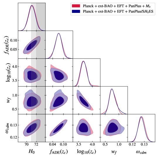
Figure 6: 2D posterior distributions reconstructed from Planck + ext-BAO + EFT, either with the $M_{b}$ prior on top of the Pantheon+ likelihood, or with the cross-correlation between the Pantheon+ data and the S$H_{0}$ES data (namely the Pantheon+/S$H_{0}$ES likelihood) as provided in Ref. Riess et al. (2021). The gray band corresponds to the $H_{0}$ constraint associated with the $M_{b}$ prior, $H_{0}=(73.04\pm 1.04)$ km/s/Mpc Riess et al. (2021).

Appendix B $\chi^{2}$ table

In this appendix, we report the best-fit $\chi^{2}$ per experiment for the $\Lambda$CDM model, the ADE model, as well as the axion-like EDE model for several combinations of data.

Data	Model	$\chi^{2}$ tot	P18TTTEE	P18lens	ext-BAO	BOSS	eBOSS	Pan	$M_{b}$	PanPlus/S$H_{0}$ES
BAO/$f\sigma_{8}$+Pan	$\Lambda$CDM	3816.39	2763.03	8.87	1.38	6.15	9.88	1027.07	–	–
	ADE	3812.50	2759.48	9.14	1.30	6.55	8.92	1027.10	–	–
	EDE	3809.87	2757.41	9.70	1.64	6.30	7.89	1026.93	–	–
BAO/$f\sigma_{8}$+Pan+$M_{b}$	$\Lambda$CDM	3847.33	2765.48	9.12	1.84	5.91	9.14	1026.89	28.94	–
	ADE	3819.06	2763.73	10.09	1.77	6.95	6.32	1026.89	3.32	–
	EDE	3812.26	2759.10	9.89	1.91	6.97	6.21	1026.87	1.31	–
EFT+Pan	$\Lambda$CDM	4020.07	2762.14	8.87	1.25	160.20	60.44	1027.17	–	–
	ADE	4018.67	2761.21	8.99	1.40	159.63	60.39	1027.06	–	–
	EDE	4017.09	2759.20	9.29	1.60	159.54	60.51	1026.95	–	–
EFT+Pan+$M_{b}$	$\Lambda$CDM	4051.76	2764.81	9.13	1.78	158.30	61.16	1026.90	29.61	–
	ADE	4026.87	2763.76	9.62	2.11	159.94	60.26	1026.86	4.33	–
	EDE	4022.83	2758.51	9.60	1.99	160.36	61.64	1026.87	3.86	–
EFT+PanPlus	$\Lambda$CDM	4404.28	2762.12	8.78	1.20	160.44	60.43	1411.31	–	–
	cADE	4404.07	2761.57	8.86	1.20	160.68	60.46	1411.31	–	–
	ADE	4402.96	2760.49	8.89	1.21	160.78	60.23	1411.36	–	–
	$c_{s}^{2}$ADE	4402.93	2760.47	8.90	1.21	160.76	60.23	1411.37	–	–
	EDE	4402.54	2758.74	9.02	1.38	160.38	61.21	1411.82	–	–
EFT+PanPlus+$M_{b}$	$\Lambda$CDM	4443.78	2766.95	9.69	1.95	158.36	60.63	1413.17	33.02	–
	cADE	4419.67	2766.20	9.67	1.92	160.68	61.17	1413.27	6.76	–
	ADE	4415.94	2763.42	9.82	1.81	160.52	60.95	1412.99	6.42	–
	$c_{s}^{2}$ADE	4415.89	2763.16	9.82	1.77	160.58	60.96	1412.91	6.70	–
	EDE	4408.67	2759.71	10.05	1.96	159.64	60.24	1413.35	3.72	–
EFT+PanPlus/S$H_{0}$ES	$\Lambda$CDM	4318.12	2767.42	9.24	2.20	158.01	60.39	–	–	1320.85
	ADE	4292.12	2763.74	9.77	1.94	160.31	60.20	–	–	1296.17

Table 3: Table of best-fit $\chi^{2}$ of the different models considered in this work for various combinations of likelihood. All datasets include Planck + ext-BAO data. Note that the columns “BOSS” and “eBOSS” refer either to the BAO/$f\sigma_{8}$ analysis or to the EFT full-shape analysis. Similarly, the column “Pan” refers to either Pantheon data or Pantheon+ data. Finally, “PanPlus/S$H_{0}$ES” corresponds to the full Pantheon+/S$H_{0}$ES likelihood as provided in Ref. Riess et al. (2021).

References

- Aghanim et al. (2020a) N. Aghanim et al. (Planck), “Planck 2018 results. VI. Cosmological parameters,” Astron. Astrophys. 641, A6 (2020a), [Erratum: Astron.Astrophys. 652, C4 (2021)], arXiv:1807.06209 [astro-ph.CO] .
- Riess et al. (2021) Adam G. Riess et al., “A Comprehensive Measurement of the Local Value of the Hubble Constant with 1 km/s/Mpc Uncertainty from the Hubble Space Telescope and the SH0ES Team,” (2021), arXiv:2112.04510 [astro-ph.CO] .
- Riess et al. (2022) Adam G. Riess, Louise Breuval, Wenlong Yuan, Stefano Casertano, Lucas M. Macri, J. Bradley Bowers, Dan Scolnic, Tristan Cantat-Gaudin, Richard I. Anderson, and Mauricio Cruz Reyes, “Cluster Cepheids with High Precision Gaia Parallaxes, Low Zero-point Uncertainties, and Hubble Space Telescope Photometry,” Astrophys. J. 938, 36 (2022), arXiv:2208.01045 [astro-ph.CO] .
- Dainotti et al. (2021) Maria Giovanna Dainotti, Biagio De Simone, Tiziano Schiavone, Giovanni Montani, Enrico Rinaldi, and Gaetano Lambiase, “On the Hubble constant tension in the SNe Ia Pantheon sample,” Astrophys. J. 912, 150 (2021), arXiv:2103.02117 [astro-ph.CO] .
- Dainotti et al. (2022) Maria Giovanna Dainotti, Biagio De Simone, Tiziano Schiavone, Giovanni Montani, Enrico Rinaldi, Gaetano Lambiase, Malgorzata Bogdan, and Sahil Ugale, “On the Evolution of the Hubble Constant with the SNe Ia Pantheon Sample and Baryon Acoustic Oscillations: A Feasibility Study for GRB-Cosmology in 2030,” Galaxies 10, 24 (2022), arXiv:2201.09848 [astro-ph.CO] .
- Mortsell et al. (2022a) Edvard Mortsell, Ariel Goobar, Joel Johansson, and Suhail Dhawan, “Sensitivity of the Hubble Constant Determination to Cepheid Calibration,” Astrophys. J. 933, 212 (2022a), arXiv:2105.11461 [astro-ph.CO] .
- Mortsell et al. (2022b) Edvard Mortsell, Ariel Goobar, Joel Johansson, and Suhail Dhawan, “The Hubble Tension Revisited: Additional Local Distance Ladder Uncertainties,” Astrophys. J. 935, 58 (2022b), arXiv:2106.09400 [astro-ph.CO] .
- Follin and Knox (2018) Brent Follin and Lloyd Knox, “Insensitivity of the distance ladder Hubble constant determination to Cepheid calibration modelling choices,” Mon. Not. Roy. Astron. Soc. 477, 4534–4542 (2018), arXiv:1707.01175 [astro-ph.CO] .
- Brout and Scolnic (2021) Dillon Brout and Daniel Scolnic, “It’s Dust: Solving the Mysteries of the Intrinsic Scatter and Host-galaxy Dependence of Standardized Type Ia Supernova Brightnesses,” Astrophys. J. 909, 26 (2021), arXiv:2004.10206 [astro-ph.CO] .
- Bernal et al. (2016) Jose Luis Bernal, Licia Verde, and Adam G. Riess, “The trouble with ,” JCAP 1610, 019 (2016), arXiv:1607.05617 [astro-ph.CO] .
- Aylor et al. (2019) Kevin Aylor, MacKenzie Joy, Lloyd Knox, Marius Millea, Srinivasan Raghunathan, and W. L. Kimmy Wu, “Sounds Discordant: Classical Distance Ladder & CDM -based Determinations of the Cosmological Sound Horizon,” Astrophys. J. 874, 4 (2019), arXiv:1811.00537 [astro-ph.CO] .
- Knox and Millea (2020) Lloyd Knox and Marius Millea, “Hubble constant hunter’s guide,” Phys. Rev. D 101, 043533 (2020), arXiv:1908.03663 [astro-ph.CO] .
- Camarena and Marra (2021) David Camarena and Valerio Marra, “On the use of the local prior on the absolute magnitude of Type Ia supernovae in cosmological inference,” Mon. Not. Roy. Astron. Soc. 504, 5164–5171 (2021), arXiv:2101.08641 [astro-ph.CO] .
- Efstathiou (2021) George Efstathiou, “To H0 or not to H0?” arXiv e-prints (2021), arXiv:2103.08723 [astro-ph.CO] .
- Schöneberg et al. (2021) Nils Schöneberg, Guillermo Franco Abellán, Andrea Pérez Sánchez, Samuel J. Witte, Vivian Poulin, and Julien Lesgourgues, “The Olympics: A fair ranking of proposed models,” (2021), arXiv:2107.10291 [astro-ph.CO] .
- Karwal and Kamionkowski (2016) Tanvi Karwal and Marc Kamionkowski, “Dark energy at early times, the Hubble parameter, and the string axiverse,” Phys. Rev. D94, 103523 (2016), arXiv:1608.01309 [astro-ph.CO] .
- Poulin et al. (2019) Vivian Poulin, Tristan L. Smith, Tanvi Karwal, and Marc Kamionkowski, “Early Dark Energy Can Resolve The Hubble Tension,” Phys. Rev. Lett. 122, 221301 (2019), arXiv:1811.04083 [astro-ph.CO] .
- Smith et al. (2020) Tristan L. Smith, Vivian Poulin, and Mustafa A. Amin, “Oscillating scalar fields and the Hubble tension: a resolution with novel signatures,” Phys. Rev. D 101, 063523 (2020), arXiv:1908.06995 [astro-ph.CO] .
- Niedermann and Sloth (2019) Florian Niedermann and Martin S. Sloth, “New Early Dark Energy,” (2019), arXiv:1910.10739 [astro-ph.CO] .
- Niedermann and Sloth (2020) Florian Niedermann and Martin S. Sloth, “Resolving the Hubble Tension with New Early Dark Energy,” (2020), arXiv:2006.06686 [astro-ph.CO] .
- Ye and Piao (2020) Gen Ye and Yun-Song Piao, “Is the Hubble tension a hint of AdS phase around recombination?” Phys. Rev. D 101, 083507 (2020), arXiv:2001.02451 [astro-ph.CO] .
- Agrawal et al. (2019) Prateek Agrawal, Francis-Yan Cyr-Racine, David Pinner, and Lisa Randall, “Rock ’n’ Roll Solutions to the Hubble Tension,” (2019), arXiv:1904.01016 [astro-ph.CO] .
- Berghaus and Karwal (2020) Kim V. Berghaus and Tanvi Karwal, “Thermal Friction as a Solution to the Hubble Tension,” Phys. Rev. D 101, 083537 (2020), arXiv:1911.06281 [astro-ph.CO] .
- Braglia et al. (2020) Matteo Braglia, William T. Emond, Fabio Finelli, A. Emir Gumrukcuoglu, and Kazuya Koyama, “Unified framework for early dark energy from -attractors,” Phys. Rev. D 102, 083513 (2020), arXiv:2005.14053 [astro-ph.CO] .
- Braglia et al. (2021) Matteo Braglia, Mario Ballardini, Fabio Finelli, and Kazuya Koyama, “Early modified gravity in light of the tension and LSS data,” Phys. Rev. D 103, 043528 (2021), arXiv:2011.12934 [astro-ph.CO] .
- Gonzalez et al. (2020) Mark Gonzalez, Mark P. Hertzberg, and Fabrizio Rompineve, “Ultralight Scalar Decay and the Hubble Tension,” (2020), arXiv:2006.13959 [astro-ph.CO] .
- Poulin et al. (2023) Vivian Poulin, Tristan L. Smith, and Tanvi Karwal, “The Ups and Downs of Early Dark Energy solutions to the Hubble tension: a review of models, hints and constraints circa 2023,” (2023), arXiv:2302.09032 [astro-ph.CO] .
- Di Valentino et al. (2021) Eleonora Di Valentino, Olga Mena, Supriya Pan, Luca Visinelli, Weiqiang Yang, Alessandro Melchiorri, David F. Mota, Adam G. Riess, and Joseph Silk, “In the realm of the Hubble tension—a review of solutions,” Class. Quant. Grav. 38, 153001 (2021), arXiv:2103.01183 [astro-ph.CO] .
- Lin et al. (2019) Meng-Xiang Lin, Giampaolo Benevento, Wayne Hu, and Marco Raveri, “Acoustic Dark Energy: Potential Conversion of the Hubble Tension,” Phys. Rev. D100, 063542 (2019), arXiv:1905.12618 [astro-ph.CO] .
- Lin et al. (2020) Meng-Xiang Lin, Wayne Hu, and Marco Raveri, “Testing in Acoustic Dark Energy with Planck and ACT Polarization,” Phys. Rev. D 102, 123523 (2020), arXiv:2009.08974 [astro-ph.CO] .
- Alam et al. (2017) Shadab Alam et al. (BOSS), “The clustering of galaxies in the completed SDSS-III Baryon Oscillation Spectroscopic Survey: cosmological analysis of the DR12 galaxy sample,” Mon. Not. Roy. Astron. Soc. 470, 2617–2652 (2017), arXiv:1607.03155 [astro-ph.CO] .
- Alam et al. (2021) Shadab Alam et al. (eBOSS), “Completed SDSS-IV extended Baryon Oscillation Spectroscopic Survey: Cosmological implications from two decades of spectroscopic surveys at the Apache Point Observatory,” Phys. Rev. D 103, 083533 (2021), arXiv:2007.08991 [astro-ph.CO] .
- Brout et al. (2022) Dillon Brout et al., “The Pantheon+ Analysis: Cosmological Constraints,” (2022), arXiv:2202.04077 [astro-ph.CO] .
- Anastasiou et al. (2022) Charalampos Anastasiou, Diogo P. L. Bragança, Leonardo Senatore, and Henry Zheng, “Efficiently evaluating loop integrals in the EFTofLSS using QFT integrals with massive propagators,” (2022), arXiv:2212.07421 [astro-ph.CO] .
- Baumann et al. (2012) Daniel Baumann, Alberto Nicolis, Leonardo Senatore, and Matias Zaldarriaga, “Cosmological Non-Linearities as an Effective Fluid,” JCAP 07, 051 (2012), arXiv:1004.2488 [astro-ph.CO] .
- Carrasco et al. (2012) John Joseph M. Carrasco, Mark P. Hertzberg, and Leonardo Senatore, “The Effective Field Theory of Cosmological Large Scale Structures,” JHEP 09, 082 (2012), arXiv:1206.2926 [astro-ph.CO] .
- Senatore and Zaldarriaga (2015) Leonardo Senatore and Matias Zaldarriaga, “The IR-resummed Effective Field Theory of Large Scale Structures,” JCAP 02, 013 (2015), arXiv:1404.5954 [astro-ph.CO] .
- Senatore (2015) Leonardo Senatore, “Bias in the Effective Field Theory of Large Scale Structures,” JCAP 11, 007 (2015), arXiv:1406.7843 [astro-ph.CO] .
- Senatore and Zaldarriaga (2014) Leonardo Senatore and Matias Zaldarriaga, “Redshift Space Distortions in the Effective Field Theory of Large Scale Structures,” (2014), arXiv:1409.1225 [astro-ph.CO] .
- Perko et al. (2016) Ashley Perko, Leonardo Senatore, Elise Jennings, and Risa H. Wechsler, “Biased Tracers in Redshift Space in the EFT of Large-Scale Structure,” (2016), arXiv:1610.09321 [astro-ph.CO] .
- D’Amico et al. (2020a) Guido D’Amico, Jérôme Gleyzes, Nickolas Kokron, Katarina Markovic, Leonardo Senatore, Pierre Zhang, Florian Beutler, and Héctor Gil-Marín, “The Cosmological Analysis of the SDSS/BOSS data from the Effective Field Theory of Large-Scale Structure,” JCAP 05, 005 (2020a), arXiv:1909.05271 [astro-ph.CO] .
- Simon et al. (2023a) Théo Simon, Pierre Zhang, and Vivian Poulin, “Cosmological inference from the EFTofLSS: the eBOSS QSO full-shape analysis,” JCAP 07, 041 (2023a), arXiv:2210.14931 [astro-ph.CO] .
- Colas et al. (2020) Thomas Colas, Guido D’amico, Leonardo Senatore, Pierre Zhang, and Florian Beutler, “Efficient Cosmological Analysis of the SDSS/BOSS data from the Effective Field Theory of Large-Scale Structure,” JCAP 06, 001 (2020), arXiv:1909.07951 [astro-ph.CO] .
- D’Amico et al. (2020b) Guido D’Amico, Leonardo Senatore, and Pierre Zhang, “Limits on CDM from the EFTofLSS with the PyBird code,” (2020b), arXiv:2003.07956 [astro-ph.CO] .
- D’Amico et al. (2020c) Guido D’Amico, Yaniv Donath, Leonardo Senatore, and Pierre Zhang, “Limits on Clustering and Smooth Quintessence from the EFTofLSS,” (2020c), arXiv:2012.07554 [astro-ph.CO] .
- Simon et al. (2022) Théo Simon, Guillermo Franco Abellán, Peizhi Du, Vivian Poulin, and Yuhsin Tsai, “Constraining decaying dark matter with BOSS data and the effective field theory of large-scale structures,” Phys. Rev. D 106, 023516 (2022), arXiv:2203.07440 [astro-ph.CO] .
- Simon et al. (2023b) Théo Simon, Pierre Zhang, Vivian Poulin, and Tristan L. Smith, “Consistency of effective field theory analyses of the BOSS power spectrum,” Phys. Rev. D 107, 123530 (2023b), arXiv:2208.05929 [astro-ph.CO] .
- Chen et al. (2022) Shi-Fan Chen, Zvonimir Vlah, and Martin White, “A new analysis of galaxy 2-point functions in the BOSS survey, including full-shape information and post-reconstruction BAO,” JCAP 02, 008 (2022), arXiv:2110.05530 [astro-ph.CO] .
- Zhang et al. (2022) Pierre Zhang, Guido D’Amico, Leonardo Senatore, Cheng Zhao, and Yifu Cai, “BOSS Correlation Function analysis from the Effective Field Theory of Large-Scale Structure,” JCAP 02, 036 (2022), arXiv:2110.07539 [astro-ph.CO] .
- Philcox and Ivanov (2022) Oliver H. E. Philcox and Mikhail M. Ivanov, “BOSS DR12 full-shape cosmology: CDM constraints from the large-scale galaxy power spectrum and bispectrum monopole,” Phys. Rev. D 105, 043517 (2022), arXiv:2112.04515 [astro-ph.CO] .
- Kumar et al. (2022) Suresh Kumar, Rafael C. Nunes, and Priya Yadav, “Updating non-standard neutrinos properties with Planck-CMB data and full-shape analysis of BOSS and eBOSS galaxies,” JCAP 09, 060 (2022), arXiv:2205.04292 [astro-ph.CO] .
- Nunes et al. (2022) Rafael C. Nunes, Sunny Vagnozzi, Suresh Kumar, Eleonora Di Valentino, and Olga Mena, “New tests of dark sector interactions from the full-shape galaxy power spectrum,” Phys. Rev. D 105, 123506 (2022), arXiv:2203.08093 [astro-ph.CO] .
- Laguë et al. (2021) Alex Laguë, J. Richard Bond, Renée Hložek, Keir K. Rogers, David J. E. Marsh, and Daniel Grin, “Constraining Ultralight Axions with Galaxy Surveys,” (2021), arXiv:2104.07802 [astro-ph.CO] .
- Smith et al. (2022) Tristan L. Smith, Vivian Poulin, and Théo Simon, “Assessing the robustness of sound horizon-free determinations of the Hubble constant,” (2022), arXiv:2208.12992 [astro-ph.CO] .
- Moretti et al. (2023) Chiara Moretti, Maria Tsedrik, Pedro Carrilho, and Alkistis Pourtsidou, “Modified gravity and massive neutrinos: constraints from the full shape analysis of BOSS galaxies and forecasts for Stage IV surveys,” (2023), arXiv:2306.09275 [astro-ph.CO] .
- Rubira et al. (2023) Henrique Rubira, Asmaa Mazoun, and Mathias Garny, “Full-shape BOSS constraints on dark matter interacting with dark radiation and lifting the S8 tension,” JCAP 01, 034 (2023), arXiv:2209.03974 [astro-ph.CO] .
- Schöneberg et al. (2023) Nils Schöneberg, Guillermo Franco Abellán, Théo Simon, Alexa Bartlett, Yashvi Patel, and Tristan L. Smith, “The weak, the strong and the ugly – A comparative analysis of interacting stepped dark radiation,” (2023), arXiv:2306.12469 [astro-ph.CO] .
- Holm et al. (2023) Emil Brinch Holm, Laura Herold, Théo Simon, Elisa G. M. Ferreira, Steen Hannestad, Vivian Poulin, and Thomas Tram, “Bayesian and frequentist investigation of prior effects in EFTofLSS analyses of full-shape BOSS and eBOSS data,” (2023), arXiv:2309.04468 [astro-ph.CO] .
- Simon et al. (2023c) Théo Simon, Pierre Zhang, Vivian Poulin, and Tristan L. Smith, “Updated constraints from the effective field theory analysis of the BOSS power spectrum on early dark energy,” Phys. Rev. D 107, 063505 (2023c), arXiv:2208.05930 [astro-ph.CO] .
- Poulin et al. (2018) Vivian Poulin, Tristan L. Smith, Daniel Grin, Tanvi Karwal, and Marc Kamionkowski, “Cosmological implications of ultralight axionlike fields,” Phys. Rev. D98, 083525 (2018), arXiv:1806.10608 [astro-ph.CO] .
- Armendariz-Picon et al. (2001) C. Armendariz-Picon, Viatcheslav F. Mukhanov, and Paul J. Steinhardt, “Essentials of k essence,” Phys. Rev. D 63, 103510 (2001), arXiv:astro-ph/0006373 .
- Gordon and Hu (2004) Christopher Gordon and Wayne Hu, “A Low CMB quadrupole from dark energy isocurvature perturbations,” Phys. Rev. D 70, 083003 (2004), arXiv:astro-ph/0406496 .
- Turner (1983) Michael S. Turner, “Coherent scalar-field oscillations in an expanding universe,” Phys. Rev. D 28, 1243–1247 (1983).
- Ma and Bertschinger (1995) Chung-Pei Ma and Edmund Bertschinger, “Cosmological perturbation theory in the synchronous and conformal Newtonian gauges,” Astrophys. J. 455, 7–25 (1995), arXiv:astro-ph/9506072 .
- Brinckmann and Lesgourgues (2018) Thejs Brinckmann and Julien Lesgourgues, “MontePython 3: boosted MCMC sampler and other features,” (2018), arXiv:1804.07261 [astro-ph.CO] .
- Audren et al. (2013) Benjamin Audren, Julien Lesgourgues, Karim Benabed, and Simon Prunet, “Conservative Constraints on Early Cosmology: an illustration of the Monte Python cosmological parameter inference code,” JCAP 1302, 001 (2013), arXiv:1210.7183 [astro-ph.CO] .
- Lesgourgues (2011) Julien Lesgourgues, “The Cosmic Linear Anisotropy Solving System (CLASS) I: Overview,” (2011), arXiv:1104.2932 [astro-ph.IM] .
- Blas et al. (2011) Diego Blas, Julien Lesgourgues, and Thomas Tram, “The Cosmic Linear Anisotropy Solving System (CLASS) II: Approximation schemes,” JCAP 1107, 034 (2011), arXiv:1104.2933 [astro-ph.CO] .
- Aghanim et al. (2020b) N. Aghanim et al. (Planck), “Planck 2018 results. V. CMB power spectra and likelihoods,” Astron. Astrophys. 641, A5 (2020b), arXiv:1907.12875 [astro-ph.CO] .
- Aghanim et al. (2020c) N. Aghanim et al. (Planck), “Planck 2018 results. VIII. Gravitational lensing,” Astron. Astrophys. 641, A8 (2020c), arXiv:1807.06210 [astro-ph.CO] .
- Beutler et al. (2011) Florian Beutler, Chris Blake, Matthew Colless, D. Heath Jones, Lister Staveley-Smith, Lachlan Campbell, Quentin Parker, Will Saunders, and Fred Watson, “The 6dF Galaxy Survey: Baryon Acoustic Oscillations and the Local Hubble Constant,” Mon. Not. Roy. Astron. Soc. 416, 3017–3032 (2011), arXiv:1106.3366 [astro-ph.CO] .
- Ross et al. (2015) Ashley J. Ross, Lado Samushia, Cullan Howlett, Will J. Percival, Angela Burden, and Marc Manera, “The clustering of the SDSS DR7 main Galaxy sample – I. A 4 per cent distance measure at ,” Mon. Not. Roy. Astron. Soc. 449, 835–847 (2015), arXiv:1409.3242 [astro-ph.CO] .
- Gil-Marín et al. (2016) Héctor Gil-Marín et al., “The clustering of galaxies in the SDSS-III Baryon Oscillation Spectroscopic Survey: BAO measurement from the LOS-dependent power spectrum of DR12 BOSS galaxies,” Mon. Not. Roy. Astron. Soc. 460, 4210–4219 (2016), arXiv:1509.06373 [astro-ph.CO] .
- Kitaura et al. (2016) Francisco-Shu Kitaura et al., “The clustering of galaxies in the SDSS-III Baryon Oscillation Spectroscopic Survey: mock galaxy catalogues for the BOSS Final Data Release,” Mon. Not. Roy. Astron. Soc. 456, 4156–4173 (2016), arXiv:1509.06400 [astro-ph.CO] .
- Reid et al. (2016) Beth Reid et al., “SDSS-III Baryon Oscillation Spectroscopic Survey Data Release 12: galaxy target selection and large scale structure catalogues,” Mon. Not. Roy. Astron. Soc. 455, 1553–1573 (2016), arXiv:1509.06529 [astro-ph.CO] .
- Ross et al. (2020) Ashley J. Ross et al., “The Completed SDSS-IV extended Baryon Oscillation Spectroscopic Survey: Large-scale structure catalogues for cosmological analysis,” Mon. Not. Roy. Astron. Soc. 498, 2354–2371 (2020), arXiv:2007.09000 [astro-ph.CO] .
- Chuang et al. (2015) Chia-Hsun Chuang, Francisco-Shu Kitaura, Francisco Prada, Cheng Zhao, and Gustavo Yepes, “EZmocks: extending the Zel’dovich approximation to generate mock galaxy catalogues with accurate clustering statistics,” Mon. Not. Roy. Astron. Soc. 446, 2621–2628 (2015), arXiv:1409.1124 [astro-ph.CO] .
- Beutler and McDonald (2021) Florian Beutler and Patrick McDonald, “Unified galaxy power spectrum measurements from 6dFGS, BOSS, and eBOSS,” JCAP 11, 031 (2021), arXiv:2106.06324 [astro-ph.CO] .
- Hou et al. (2020) Jiamin Hou et al., “The Completed SDSS-IV extended Baryon Oscillation Spectroscopic Survey: BAO and RSD measurements from anisotropic clustering analysis of the Quasar Sample in configuration space between redshift 0.8 and 2.2,” Mon. Not. Roy. Astron. Soc. 500, 1201–1221 (2020), arXiv:2007.08998 [astro-ph.CO] .
- Scolnic et al. (2018) D. M. Scolnic et al., “The Complete Light-curve Sample of Spectroscopically Confirmed SNe Ia from Pan-STARRS1 and Cosmological Constraints from the Combined Pantheon Sample,” Astrophys. J. 859, 101 (2018), arXiv:1710.00845 [astro-ph.CO] .
- Mead et al. (2020) Alexander Mead, Samuel Brieden, Tilman Tröster, and Catherine Heymans, “HMcode-2020: Improved modelling of non-linear cosmological power spectra with baryonic feedback,” (2020), 10.1093/mnras/stab082, arXiv:2009.01858 [astro-ph.CO] .
- Lewis (2019) Antony Lewis, “GetDist: a Python package for analysing Monte Carlo samples,” (2019), arXiv:1910.13970 [astro-ph.IM] .
- Raveri and Hu (2019) Marco Raveri and Wayne Hu, “Concordance and discordance in cosmology,” Phys. Rev. D 99, 043506 (2019), arXiv:1806.04649 [astro-ph.CO] .
- Riess et al. (2019) Adam G. Riess, Stefano Casertano, Wenlong Yuan, Lucas M. Macri, and Dan Scolnic, “Large Magellanic Cloud Cepheid Standards Provide a 1% Foundation for the Determination of the Hubble Constant and Stronger Evidence for Physics beyond CDM,” Astrophys. J. 876, 85 (2019), arXiv:1903.07603 [astro-ph.CO] .