Sky location of Galactic white dwarf binaries in space-based gravitational wave detection

Abstract

Quickly localizing the identified white dwarf (WD) binaries is the basic requirement for the space-based gravitational wave (GW) detection. In fact, the amplitude of GW signals are modulated by the periodic motion of GW detectors on the solar orbit. The intensity of the observed signals is enhanced according to the observation time beyond a year to enhance a high signal to noise ratio (SNR). As data gap exists, the completeness of the data observed for a long time depends on filling gaps in the data. Actually, in a year period, the GW sources have a best observation orbit position of GW detectors, where the intensity of GW is maximum. Thus, the best positions can be searched for the verified GW sources of the sky map to enhance SNR too, which avoids filling data gaps. For the three arms response intensity of the GW signals changing more clearly with the location of the GW sources relative to the detector, the noises and the suppression of noise by time delay interferometer are ignored. As a verification case, the four WD binaries are chosen, whose best observation orbit positions of the GW detectors are related to the direction of WD binaries perpendicular to the detection arms. The two verification binaries: J0806 and V407 Vul are observed at the best orbit positions by TAIJI for the short time of 2 and 3 days respectively. The corresponding intensities of GWs are above the values of the TAIJI sensitivity curve, significantly. Location parameter estimation of the verification WD binaries are performed using the Metropolis-Hastings MCMC method. The confidence level of the parameters obtained in the best position is significantly several times higher than that in the worst position where the direction of WD binaries are almost parallel to the detection arms. Compared with a single detector, the network of two detectors does not significantly improve the accuracy of location of the verification binaries. The reason of that result is that one GW source can not be perpendicular to both detectors of TAIJI and LISA. These results imply that the searching of GW signals and parameter estimation of GW sources from the experimental data of the space-based mission do not ignore the orbit positions relevant to GW sources.

I Introduction

The nearly hundred events of gravitational waves above 10 Hz are observed during the observing run O1-O3 by the ground-based observatories from LIGO, VIRGO and KAGRA collaborations The LIGO Scientific Collaboration et al. (2021); Abbott et al. (2023). The gravitational wave observation below 1 Hz is a space-based mission matching the longer arms with the order of $10^{6}$ km apart between the spacecraftsRuan et al. (2020a), such as LISA Baker et al. (2007); Amaro-Seoane et al. (2017) and TAIJI Hu and Wu (2017). The gravitational wave sources detected by the ground-based observatories and the space-based mission have the different responses to the detection arms. The cross-correlated response of the Hanford and Livingston LIGO detectors is modulated as the rotation of the Earth sweeps the antenna pattern across the skyAllen and Ottewill (1997); Cornish (2001). Referring to the configuration of LISA Baker et al. (2007); Amaro-Seoane et al. (2017) and TAIJI Hu and Wu (2017), the space-based observatories consist of a triangular structure of three spacecrafts in a heliocentric orbit with an arm length of the million kilometers. The three spacecrafts orbit Kepler, with the same annual period as Earth, have two forms of motion, one is the revolution of the heliocentric orbit, and the other is the rotation of three spacecraft around the center of the triangleRuan et al. (2020a). The relative velocity between the two spacecrafts causes Doppler shift of the photon emitted by the first spacecraft and received by the second. The heterodyne interferometry is required to track the relative displacement between two spacecrafts. The on-orbit detectors have maximal response of the gravitational wave as a transverse wave, when the propagation orientation of the gravitational wave source is perpendicular to the sides of a triangle made up of three spacecrafts. On the contrary, if it is parallel, there is almost no response. Thus, The amplitude of gravitational waves is modulated with a year period.

The orbital modulation effect of the observed gravitational wave signals is described by the detector response function. The full LISA response function to an arbitrary gravitational wave is derived using a coordinate free approach in the transverse-traceless gaugeCornish and Rubbo (2003). The forward modeling of space-based gravitational wave detectors was proposed and an adiabatic approximation to the detector response significantly extends the range of the standard low frequency approximationRubbo et al. (2004). Recently, a time-domain generic response code LISA gravitational wave Response(Bayle et al., 2022) is proposed for projecting the gravitational wave polarizations onto the LISA constellation arms. In this paper, the TAIJI response function is expressed in the transverse-traceless gauge. The length of on-orbit detection arms in space-time is calculated numerically in the time domain.

The GW signals from Massive Black Hole merging linger for much longer in the detector sensitive band, which overlap with the continuous and nearly monochromatic GW signals of WD binaries. The data analysis of those overlapping signals is one of the Mock LISA Data ChallengesBabak et al. (2009). These overlapped signals cross the entire TAIJI frequency spectrum too. In fact, for the third-generation ground-based detectors the signals from different sources will be simultaneously present in the data, whose associated computational challenges have recently begunSperi et al. (2022). The data analysis of overlapped GW signals become already a general issue to be solved. The TAIJI Data Challenges (TDC) are online for the solution of that issueRen et al. (2023). Considering the location parameters of the detectors, the overlapped GW signals may be degenerated slightly for a verification source.

Among all kinds of ultra-compact stellar mass binaries, white dwarf binariess comprise the absolute majority (up to $10^{8}$) in the Milky Way. Being abundant and nearby, DWDs are expected to be the most numerous gravitational wave sources for space-based detectors Nelemans et al. (2001a); Yu and Jeffery (2010); Breivik et al. (2020); Lamberts et al. (2018). There are many predictions based on a Galaxy model combined with a binary population model (Nelemans et al., 2001b; Nelemans et al., 2004; Nissanke et al., 2012; Ruiter et al., 2010; Postnov and Yungelson, 2014; Toonen et al., 2017). Recently, more studies construct an observationally driven population (Korol et al., 2017; Breivik et al., 2020; Korol et al., 2019, 2021). The numerous monochromatic gravitational waves emitted by the Galactic DWDs form the foreground signals of sky map. In these sources the verification binaries signals such as J0806, V407 Vul, ES Cet and SDSSJ1351(abbr of SDSSJ135154.46-064309.0) have been discovered by X-ray and optical observatories Kupfer et al. (2018). These binary sources have the rotational period ranging from a few hundred to a thousand seconds, that are sensitive to the detection arms of LISA and TAIJI.

Quickly localizing the identified binaries is the basic requirement for the space-based gravitational wave detection, that is used to calibrate the detection data and reduce the noises of detectors. As three spacecrafts are moving on the solar orbit with a year period, the orientation of the identified binaries does not keep being perpendicular to the detection arms. The detection arm response intensity of the gravitational wave of the observed sources have the maximum and minimum relative to the perpendicular and parallel to detection arms. Thus, a gravitational wave source have a best observed window in a year period of orbit.

Generally, on the source location of gravitational wave signal, the intensity of the observed signal is enhanced according to the observation time (integration time) to obtain a high SNR. The observation time is generally selected as years, so the modulation effect of the detector at different orbital positions of the gravitational wave source is ignored.As the data gap exists in the whole year time, a long time observation data need filling the gap, which takes deviation from the real dataSperi et al. (2022). In this paper, we consider the modulation effect of the detector, i.e., the orbit position of space-based laser interferometer detectors, have significant effects on the the localizing the sky position of the identified binaries. For the three arms response intensity of the GW signals changing more clearly with the location of the GW sources relative to the detector, the noises and the suppression of noise by time delay interferometer are ignored. We focus on the projected signal on the single arm detector of an identified WD binary. So, instead of a few years, observation time was replaced with a short one.

Localizing the sky position of the gravitational wave source is a key scientific goal for gravitational wave observations(Błaut, 2011). There are two major methods for localizing the sky position of GW sources. One method is the Fisher information matrix approximation (FIM), which can give robust estimation of the sky localization of the source with a high SNR where the inverse of FIM gives the covariance matrix of the parameters. Another method is the Bayesian estimation i.e. the posterior distribution expressing the uncertainty of the source parameters(Shuman and Cornish, 2022). The angular resolution is often chosen as the sky localization accuracy for an arbitrary network of interferometric gravitational-wave (GW) detectors(Wen and Chen, 2010). Angular resolution of the detector and the estimation errors of the signal’s parameters in the high frequency regimes are calculated as functions of the position in the sky and as functions of the frequency(Zhang et al., 2021). In addition, detectors configuration properties, such as the orientation change of the detector plane, can also effect the angular resolution(Zhang et al., 2021). Besides, the network for different two detectors can effectively help to get better accuracy in the sky localization. As an example, similarities and complements between LISA and TAIJI imply that LISA-TAIJI network can effectively help to accurately localize GW sources, since the angular resolution measurements for the network depend on the configuration angle and separation of the two constellations(Ruan et al., 2021, 2020b). The network was estimated to improve the angular resolution for over 10 times by comparison with each individual LISA or TAIJI detector(Cutler, 1998). The LISA-TianQin network has better ability in sky localization for sources with frequencies in the range 1-100 mHz and the network has larger sky coverage for the angular resolution than the individual detector(Wang et al., 2020).

For the first time, we focus on the sky location of the identified binary sources in a short observation time, considering the amplitude modulation effect of different detector positions on the WD binary response. Due to the periodic orbit motion of the detector, the results of the short time observation are related to the orbit position of the detector. For some specific WD binary sources, the best localizing the sky position of the sources at the best detector position is achieved in this paper. As a verification case, the four WD binaries are chosen, whose best observation orbit positions of the GW detectors are related to the direction of WD binaries perpendicular to the detection arms. The two verification binaries: J0806 and V407 Vul are observed at the best orbit positions by TAIJI for the short time of 2 and 3 days respectively, whose GW intensities are greater than the values of TAIJI sensitivity curve, significantly. The other two verification binaries: Es Cet and SDSSJ1351 are beyond the sensitive cure for the observation time of 35 and 52 days respectively when the their intensities are above TAIJI sensitivity curve. Compared with a single detector, the network of two detectors does not significantly improve the accuracy of location of the verification binaries, which is different conclusion from the paper(Ruan et al., 2021, 2020b). The reason of that result is that one GW source can not be perpendicular to both detectors of TAIJI and LISA for a short observation time. For a long observation time, the network of two detectors has a significant improvement to angular resolution.

The structure of this paper is as follows: in Sec.III , we mainly introduce the signal model of the WD binary star and the distribution of its constituent parameters; in Sec.II , we mainly introduce the detector orbit and the detector response form in the time domain; in Sec.IV , the best localizing the sky position of the sources at the best detector position is achieved; in Sec.V , the full text is summarized.

II Detector response

II.1 Detector Orbit

Referring to LISA orbit, the TAIJI spacecrafts will orbit KeplerRubbo et al. (2004) and the arm length is 3$\times 10^{6}$ km, which is different from LISA arm length: 2.5 $\times 10^{6}$ km. Each spacecraft positions are expressed as a function of time. To second order in the eccentricity, the Cartesian coordinates of the spacecraft are given by

$$x(t) = R\cos(\alpha)+\frac{1}{2}eR\Big{(}\cos(2\alpha-\beta)-3\cos(\beta)\Big{)}$$

$$+\frac{1}{8}e^{2}R\Big{(}3\cos(3\alpha-2\beta)-10\cos(\alpha)$$

$$-5\cos(\alpha-2\beta)\Big{)}$$

$$y(t) = R\sin(\alpha)+\frac{1}{2}eR\Big{(}\sin(2\alpha-\beta)-3\sin(\beta)\Big{)}$$

$$+\frac{1}{8}e^{2}R\Big{(}3\sin(3\alpha-2\beta)-10\sin(\alpha)$$

$$+5\sin(\alpha-2\beta)\Big{)}$$

$$z(t) = -\sqrt{3}eR\cos(\alpha-\beta)$$ (1)

$$+\sqrt{3}e^{2}R\Big{(}\cos^{2}(\alpha-\beta)+2\sin^{2}(\alpha-\beta)\Big{)}$$

Where $R=1$ AU is the radial distance to the guiding center, $e$ is the eccentricity, $\alpha=2\pi t/1year+\kappa$ is the orbital phase of the guiding center, and $\beta=2\pi n/3+\lambda$ ($n=0,1,2$) is the relative phase of the spacecraft within the constellation. The parameters $\kappa$ and $\lambda=0$ give the initial ecliptic longitude and orientation of the constellation. The orbital eccentricity is computed based on the arm length: $e=L/(2\sqrt{3}R)$. By setting the mean arm-length equal to those of the TAIJI baseline, $L=3\times 10^{9}$ m, the spacecraft orbits are found to have an eccentricity of $e=0.005789$, which indicates that the second order effects are down by a factor of 100 relative to leading order.

II.2 Response Function

The gravitational waves are expressed as the perturbations of the flat space-time

$$g_{\mu\nu}=\eta_{\mu\nu}+h_{\mu\nu}$$ (2)

The laser link signal is emitted from the spacecraft $i$ at $t_{i}$ moment and received by the spacecraft $j$ at $t_{j}$ moment. Assume that $c=1$. Then, the distance $\ell_{ij}$ between the the laser link in space-time can be obtained Rubbo et al. (2004)

$$\ell_{ij}=\int_{i}^{j}\sqrt{g_{\mu\nu}dx^{\mu}dx^{\nu}}=\left|{\mathbf{x}_{j}(t_{j})-\mathbf{x}_{i}(t_{i})}\right|$$

$$+\frac{1}{2}\hat{r}_{ij}(t)\otimes\hat{r}_{ij}(t):\int_{i}^{j}{\bf h}(\xi(\lambda))d\lambda$$ (3)

Here $\left|\mathbf{x}-\mathbf{y}\right|$ denotes the Cartesian distance between $\mathbf{x}$ and $\mathbf{y}$ and ${\bf h}(\xi)$ is the gravitational wave tensor in the transverse-traceless gauge. The colon here denotes a double contraction, ${\bf a}:{\bf b}=a^{ij}b_{ij}$ .

$\hat{r}_{ij}(t)$ denotes the unit vector

$$\hat{r}_{ij}(t_{i})=\frac{{\bf x}_{j}(t_{j})-{\bf x}_{i}(t_{i})}{\ell_{ij}}\,.$$ (4)

So the equation is used to calculate $\delta\ell_{ij}$

$$\delta\ell_{ij}=\frac{1}{2}\hat{r}_{ij}(t)\otimes\hat{r}_{ij}(t):\int_{i}^{j}{\bf h}(\xi(\lambda))d\lambda$$ (5)

When the gravitational wave traveling in the $\hat{k}$ direction, the wave variable $\xi(\lambda)$ can be calculated by

$$\xi(\lambda)=t(\lambda)-\hat{k}\cdot{\mathbf{x}(\lambda)}$$ (6)

Explicitly, the time and position depend on the parameterization in the following way

$$t(\lambda)=t_{i}+\lambda$$

$$\mathbf{x}(\lambda)=\mathbf{x}(t_{i})+\lambda\hat{r}_{ij}(t_{i}).$$ (7)

The time and position are gotten by $d\lambda=dt$:

$$\mathbf{x}(t)=\mathbf{x}(t_{i})+(t-t_{i})\hat{r}_{ij}(t_{i})$$

$$\xi(t)=t-\hat{k}\cdot{\mathbf{x}(t)}.$$ (8)

So the Eq. (5) can be changed to the following form

$$\delta\ell_{ij}=\frac{1}{2}\hat{r}_{ij}(t)\otimes\hat{r}_{ij}(t):\int_{t_{i}}^{t_{j}}{\bf h}(t-\hat{k}\cdot{\mathbf{x}(t)})dt$$ (9)

The Eq. (9) can calculate the $\delta\ell_{ij}$ in a numerical way in the time domain.

II.3 General analysis of annual modulation effect on detectors

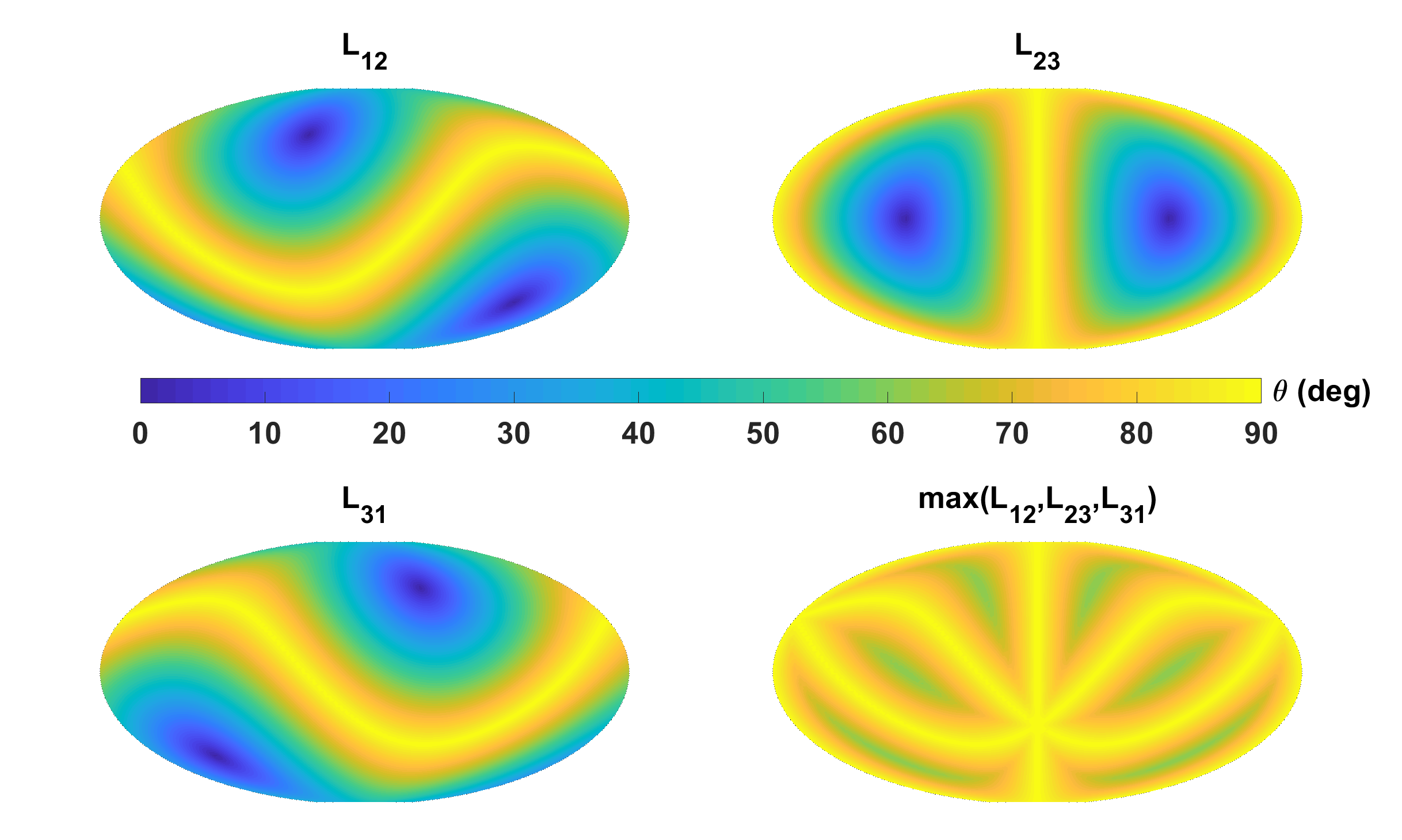
(a) $\kappa=0^{\circ}$

(b) $\kappa=45^{\circ}$

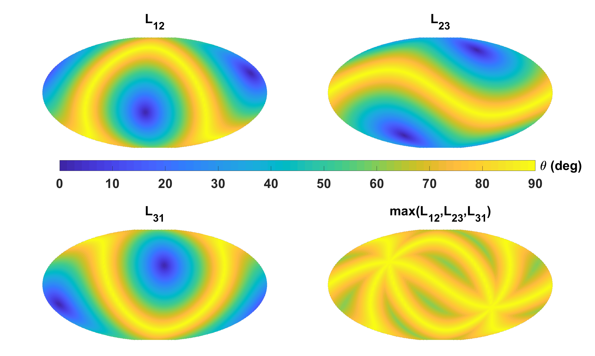
(c) $\kappa=90^{\circ}$

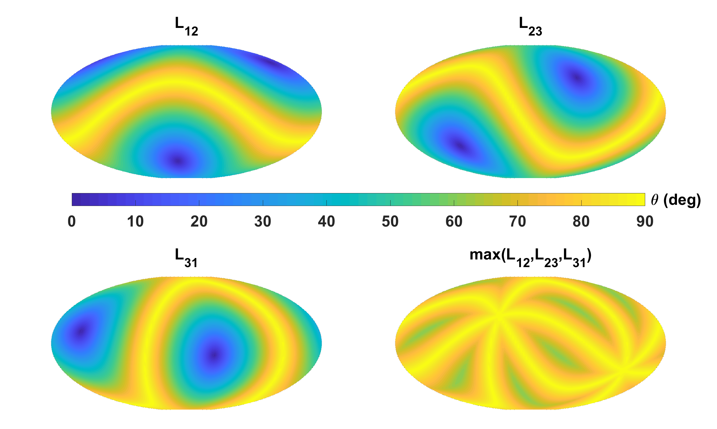
(d) $\kappa=135^{\circ}$

Figure 1: The sky map of the angle $\theta$ between GW sources in the whole space and three detection arms ($L_{12}$, $L_{23}$, and $L_{31}$) and the maximum angle $\theta$ in three detection arms ($L_{12}$, $L_{23}$, and $L_{31}$) for different variable $\kappa$ respectively. The variable $\kappa$ ($\kappa\in\left[0,2\pi\right]$) is divided into 8 equal parts. In the figure, there are four values: $0^{\circ},45^{\circ},90^{\circ},135^{\circ}$.

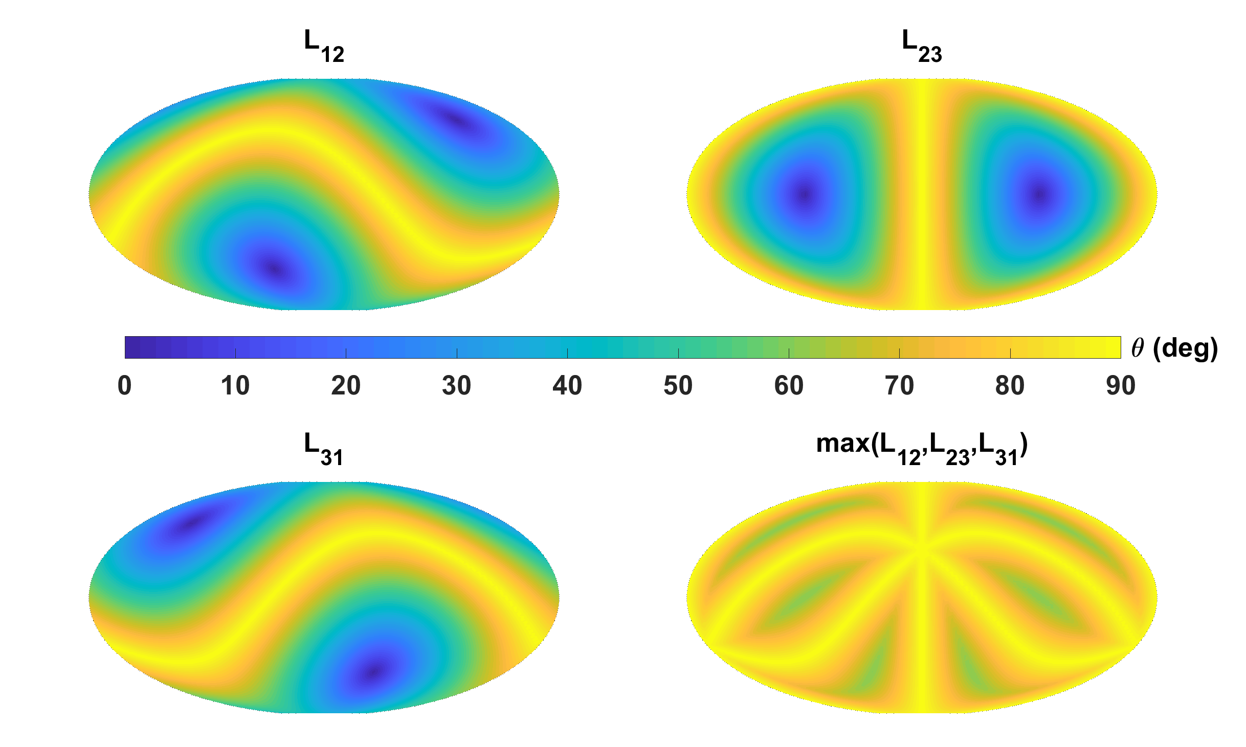
(a) $\kappa=180^{\circ}$

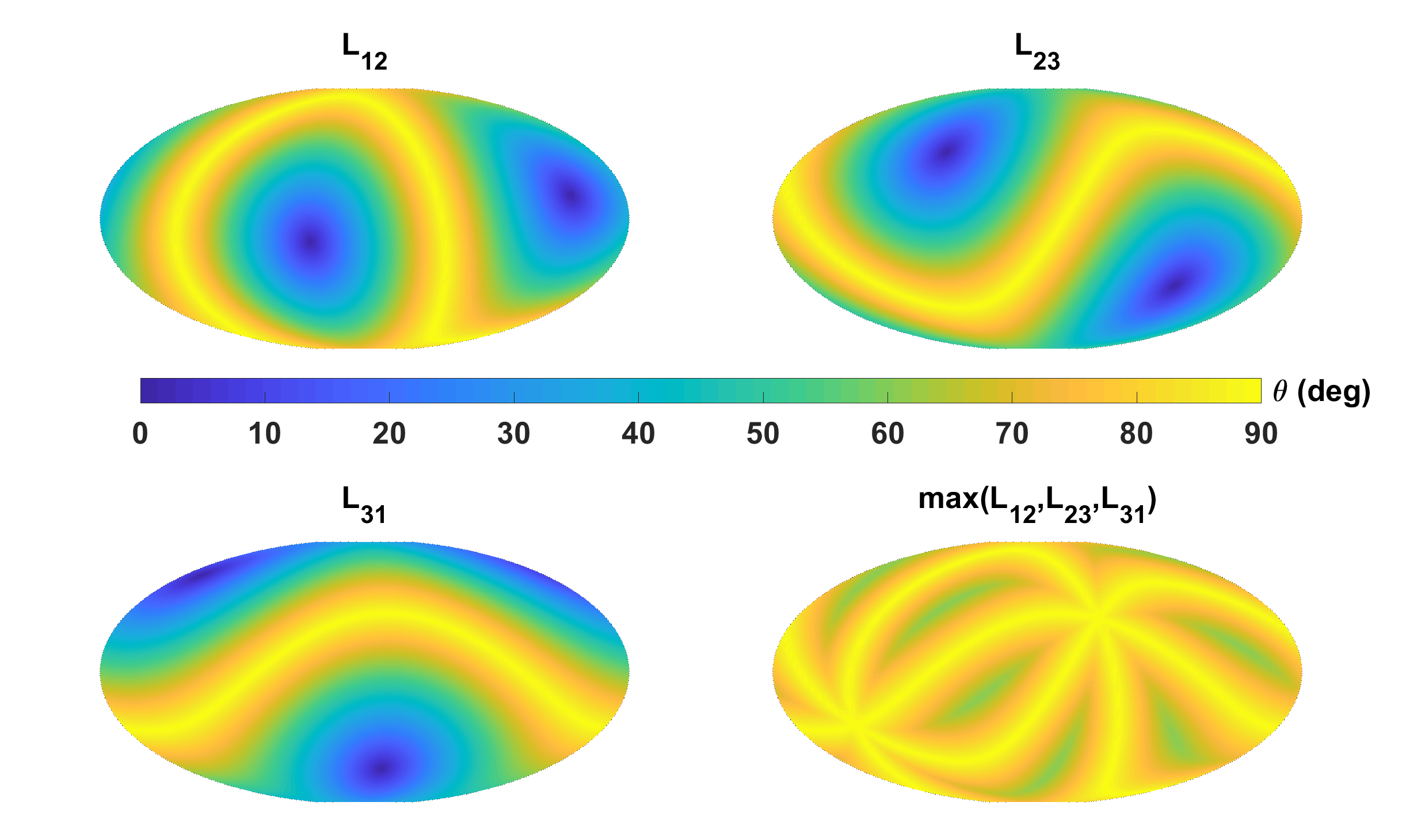
(b) $\kappa=225^{\circ}$

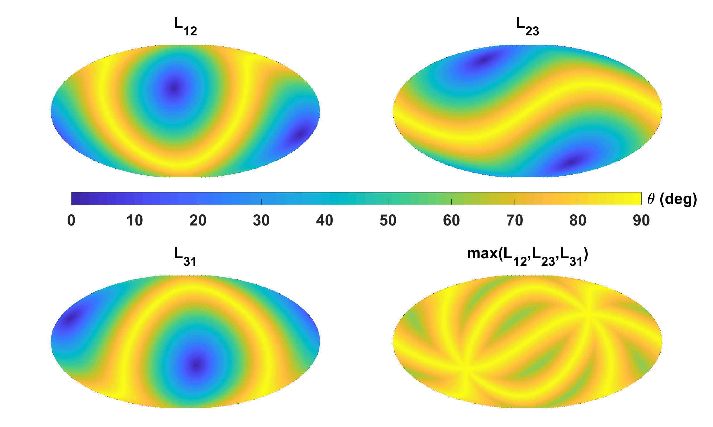
(c) $\kappa=270^{\circ}$

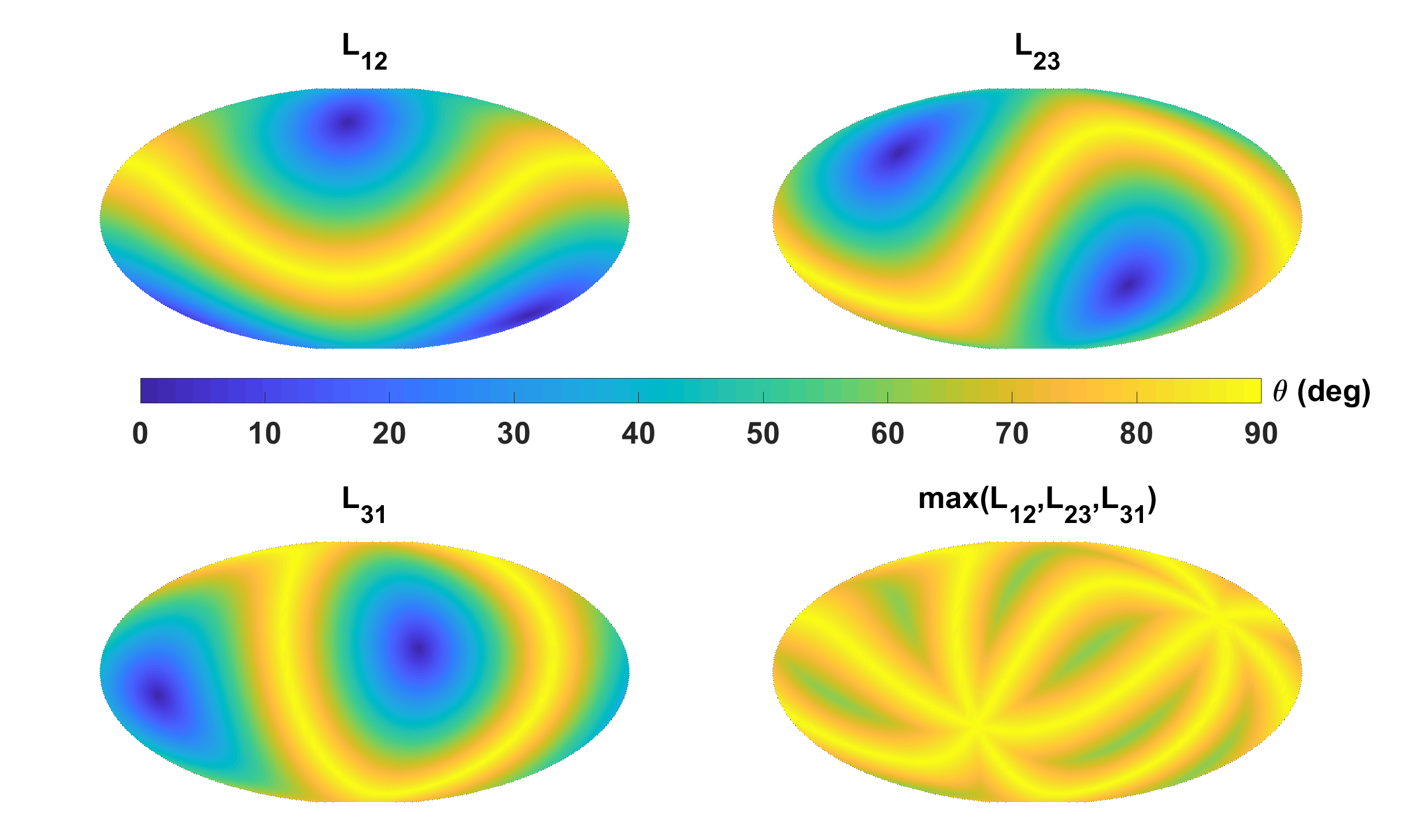
(d) $\kappa=315^{\circ}$

Figure 2: The same as Fig. 1. There are the rest four values: $180^{\circ},225^{\circ},270^{\circ},315^{\circ}$.

One year of period modulation effect is mainly relevant to the change of the angle $\theta$ between the propagation direction of gravitational wave source and the detection arm during the one-year orbit. The angle $\theta$ is gotten by the expression

$$\theta=\arccos{\left|\frac{\hat{k}\cdot\hat{r}_{ij}}{|\hat{k}|\left|\hat{r}_{ij}\right|}\right|},$$ (10)

where $\hat{k}$ is the propagation direction of the GW source and $\hat{r}_{ij}(t)$ denotes the unit vector of the detection arm.

$$\hat{r}_{ij}(t_{i})=\frac{{\bf x}_{j}(t_{j})-{\bf x}_{i}(t_{i})}{\ell_{ij}}\,.$$ (11)

Here, we set $t_{i}=0$ and $t_{j}=\ell_{ij}/C$ (C is light velocity). The angle $\theta$ is different when the detectors are at different orbit positions. In the extreme case, when the angle $\theta=0^{\circ}$, the response of the gravitational wave to the detection arms ($L_{12}$, $L_{23}$, and $L_{31}$) is the weakest; when the angle $\theta=90^{\circ}$, that response is strongest. In this case, the ecliptic longitude $\kappa$ is used to present the detector position on orbit.

The coordinates under the $SSB$ frame are composed of the spatial position($\beta,\lambda$). In every sky map, the horizontal axis represents the longitude ($\lambda\in\left[-\pi,\pi\right]$) and the vertical axis represents the ecliptic latitude ($\beta\in\left[-\pi/2,\pi/2\right]$). In Fig. 1 and Fig. 2, eight sky maps are drawn for each detection arm ($L_{12}$, $L_{23}$, and $L_{31}$), which is relevant to the variable $\kappa$ ($\kappa\in\left[0,2\pi\right]$). In Fig. 1 and Fig. 2, the single arm response only cover the parts of all sky map, which look like the twisted long bands relevant to an area greater than 60^∘. The response intensity of gravitational wave source in the area less than 60^∘ (cos 60^∘=1/2) is reduced by more than half. By combining the three arms, there are most of the sky map where the response intensity of the gravitational wave source is barely attenuated. In the sky map, there are also the overlapped parts where each response of the three arms is almost same intensity. These overlapped parts change with the the detector position expressed by the ecliptic longitude $\kappa$. In Fig. 1 and Fig. 2, there are one or two overlapped area when the detector position changes on orbit, which is relevant to the selected $\kappa$: $0^{\circ},\ 45^{\circ},\ 90^{\circ},\ 135^{\circ},\ 180^{\circ},\ 225^{\circ},\ 270^{\circ}$ and $315^{\circ}$. In the overlapped area the gravitational wave sources have maximal response to the detector arms. That means that there are the best on-orbit positrons, which is most sensitive to the gravitational wave sources.

In order to search the overlapped area in all sky map, in all orbit positions, the minimum and maximum responses, expressed with $\theta$, of the three arms are drawn in Fig. 3. As is seen in Fig. 3 that there are the orbit positions relevant to the minimum responses where the the gravitational wave source’s observation is difficult. Otherwise, there are also the orbit positions relevant to the maximum responses where the the gravitational wave source may be observed easily. In detail, there are some small sky where the $\theta$ are in the range of $70^{\circ}$ to $80^{\circ}$ . It implies that the overlapped area almost covers all sky map. Thus, The best observation position on orbit, expressed with $\kappa$, is always found for a particular gravitational wave source.

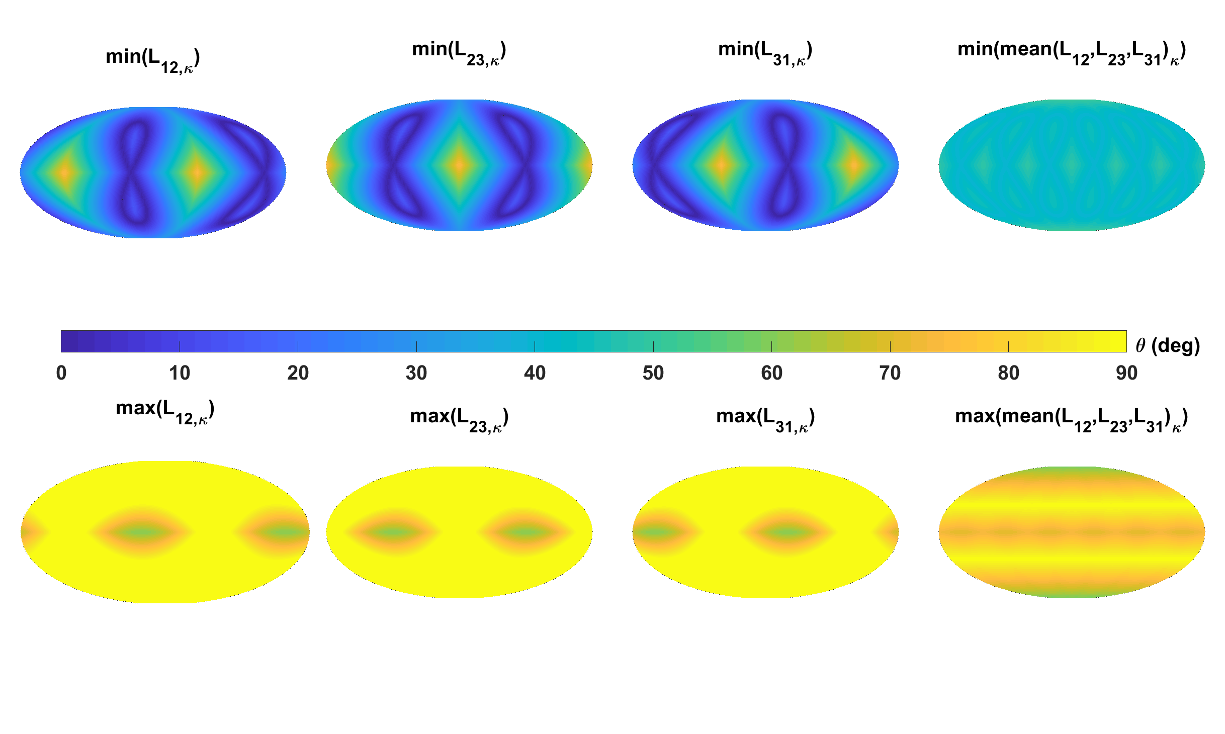
Figure 3: The sky maps of the angle $\theta$ for all $\kappa$. The top three ones are the minimum-scanning by $\kappa$ value varying, which is relevant to $L_{12,\kappa}$, $L_{23,\kappa}$ and $L_{31,\kappa}$, respectively. The top right one is the combination result with three arms. The bottom t three ones are the minimum-scanning by $\kappa$ value varying, which is relevant to $L_{12,\kappa}$, $L_{23,\kappa}$ and $L_{31,\kappa}$, respectively.The bottom right one is also the combination result.

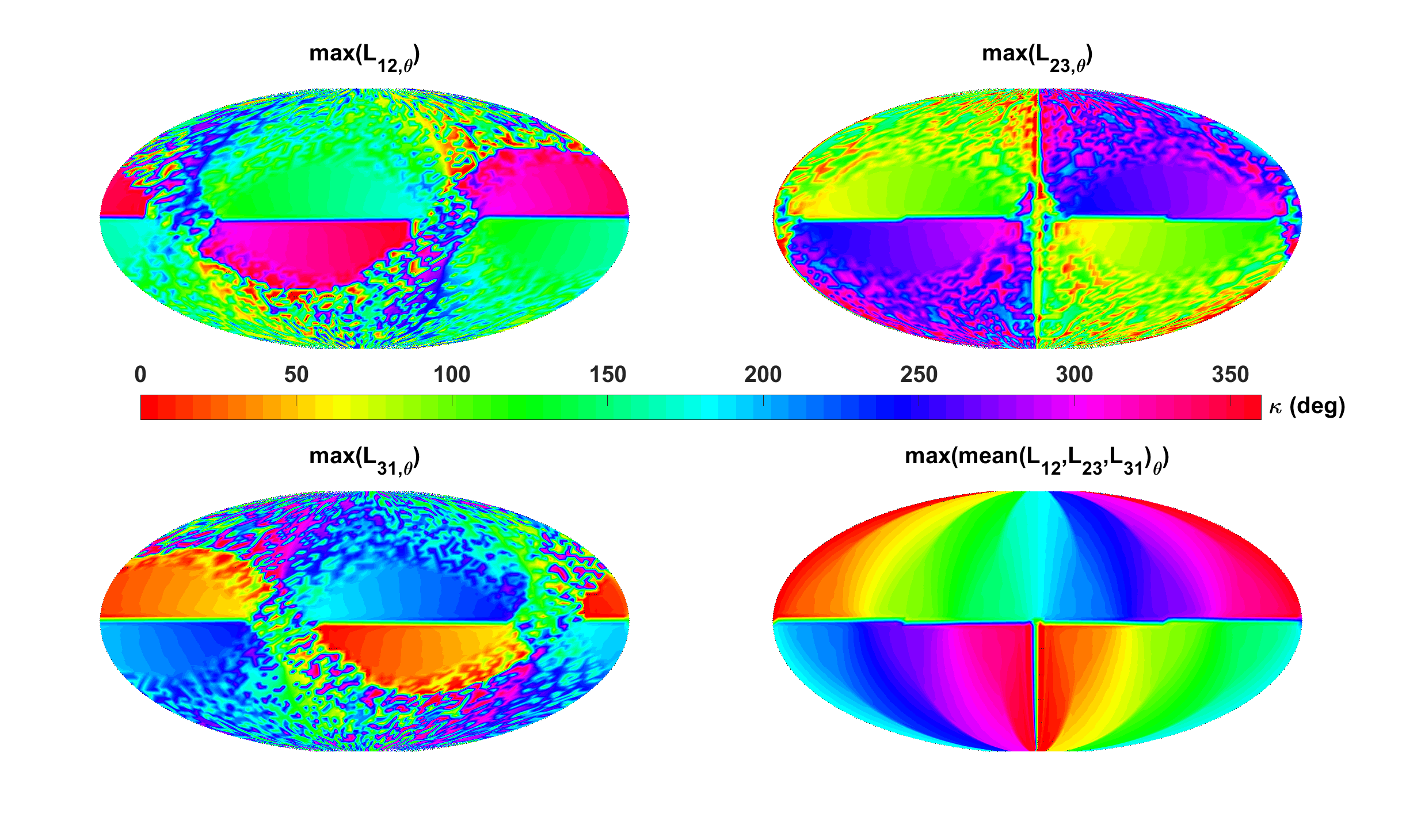
Figure 4: The sky maps of $\kappa$ at the maxmum of the Angle $\theta$ of $L_{12,\kappa}$, $L_{23,\kappa}$, $L_{31,\kappa}$, and the mean of the Angle $\theta$ of $L_{12,\kappa}$, $L_{23,\kappa}$ and $L_{31,\kappa}$ respectively.

III GALACTIC DOUBLE WHITE DWARF BINARIES

III.1 WD binary singal model

The gravitational wave signals from the WD binary are described by a set of eight parameters: frequency $f$, frequency derivative $\dot{f}$, amplitude ${\cal A}$, sky position in ecliptic coordinates $(\lambda,\beta)$, orbital inclination $\iota$, polarisation angle $\psi$, and initial orbital phase $\phi_{0}$ (Cutler, 1998; Roebber et al., 2020; Karnesis et al., 2021). The recipes for generating ${\cal A}$, $f$, $\dot{f}$, and $(\lambda,\beta)$ are based on the currently available observations. The cosine of the inclination,$\cos{\iota}$, was taken to be uniform in the range $\left[-1,1\right]$. The polarization angle $\psi$ was taken to be uniform in the range $\left[0,\pi\right]$. The initial orbital phase, $\phi_{0}$, was taken to be uniform in the range $\left[0,2\pi\right]$. The gravitational wave emitted by a monochromatic source is calculated using the quadrupole approximation Landau and Lifshitz (1962); Peters and Mathews (1963). In this approximation, the gravitational wave signals are described as a combination of the two polarizations ($+,\times$)(Korol et al., 2021):

$$h_{+}(t)=\mathcal{A}(1+\cos\iota^{2})\cos(\Phi(t))$$

$$h_{\times}(t)=2\mathcal{A}\cos\iota\sin(\Phi(t)).$$ (12)

In above expression,

$$\mathcal{A}=\frac{2(G\mathcal{M})^{5/3}}{c^{4}D_{L}}(\pi f)^{2/3}$$

$$\Phi(t)=2\pi ft+\pi\dot{f}t^{2}+\phi_{0}$$

$$\dot{f}=\frac{96}{5}\pi^{8/3}\left(\frac{G{\cal M}}{c^{3}}\right)^{5/3}f^{11/3}.$$ (13)

where $\mathcal{M}\equiv(m_{1}m_{2})^{3/5}/(m_{1}+m_{2})^{1/5}$ is the chirp mass, and $D_{L}$ is luminosity distance, and $G$ and $c$ are the gravitational constant and the speed of light, respectively. This is a source frame, but for detectors, Solar System Barycenter ($SSB$) frame, based on the ecliptic plane, is selected. In $SSB$ frame, the standard spherical coordinates $\left(\theta,\phi\right)$ and the associated spherical orthonormal basis vectors $\left(\bf{e}r,\bf{e}\theta,\bf{e}\phi\right)$ are confirmed. The position of the source in the sky is parametrized by the ecliptic latitude $\beta=\pi/2-\theta$ and the ecliptic longitude $\lambda=\phi$. The gravitational wave propagation vector $\hat{k}$ in spherical coordinates is expressed as

$$\hat{k}=-\bf{e}r=-\cos\beta\cos\lambda\,\hat{x}-\cos\beta\sin\lambda\,\hat{y}-\sin\beta\,\hat{z}\,.$$ (14)

The reference polarization vectors is the following:

$$\hat{u} = -\bf{e}\theta=-\sin\beta\cos\lambda\,\hat{x}-\sin\beta\sin\lambda\,\hat{y}+\cos\beta\,\hat{z}$$

$$\hat{v} = -\bf{e}\phi=\sin\lambda\,\hat{x}-\cos\lambda\,\hat{y}.$$ (15)

The last degree of freedom between the frames corresponds to the rotation around the line of sight, and is represented by the polarization angle $\psi$. The polarization tensors are given by

$${\mbox{\boldmath$\epsilon$}}^{+} = \cos(2\psi){\bf e}^{+}-\sin(2\psi){\bf e}^{\times}$$

$${\mbox{\boldmath$\epsilon$}}^{\times} = \sin(2\psi){\bf e}^{+}+\cos(2\psi){\bf e}^{\times}\,,$$ (16)

where the basis tensors ${\bf e}^{+}$ and ${\bf e}^{\times}$ are expressed in terms of two orthogonal unit vectors,

$${\bf e}^{+} = \hat{u}\otimes\hat{u}-\hat{v}\otimes\hat{v}$$

$${\bf e}^{\times} = \hat{u}\otimes\hat{v}+\hat{v}\otimes\hat{u}\,.$$ (17)

An arbitrary gravitational wave traveling in the $\hat{k}$ direction can be written as the linear sum of two independent polarization states,

$${\bf h}(\xi)=h_{+}(\xi){\mbox{\boldmath$\epsilon$}}^{+}+h_{\times}(\xi){\mbox{\boldmath$\epsilon$}}^{\times}\,,$$ (18)

where the wave variable $\xi=t-\hat{k}\cdot{\bf x}$ gives the surfaces of constant phase.

III.2 sky map of WD binary sources

Combining the theoretical model with the observations, the resulting new model may be more in line with the actual distribution. In the paperHollands et al. (2018), using Gaia DR2 data Brown et al. (2018), an up-to-date sample of white dwarfs within 20 pc of the Sun is presented. So the WDs are distributed in the disc according to an exponential radial stellar profile with an isothermal vertical distribution Korol et al. (2021):

$$\rho(R,z)=\rho_{{\rm WD},\odot}\,e^{-\frac{R-R_{\odot}}{R_{\rm d}}}\operatorname{sech}^{2}\left(\frac{z-z_{\odot}}{z_{\rm d}}\right),$$ (19)

where $\rho_{{\rm WD},\odot}=(4.49\pm 0.38)\times 10^{-3}$ pc^-3 is the local WD density estimated by (Hollands et al., 2018) , $0\leq R\leq 20$  kpc is the cylindrical radial coordinate measured from the Galactic centre, $-2\leq z\leq 2$  kpc is the height above the Galactic plane, $R_{\rm d}=2.5\,$kpc is the disc scale radius, and $z_{\rm d}=0.3$  kpc is the disc scale height (e.g. Jurić et al., 2008; Ted Mackereth et al., 2017). Sun’s position is set to $(R_{\odot},z_{\odot})=(8.1,0.03)$ kpc (e.g. Abuter et al., 2019).

The total number of WD stars in the Milky Way disc by integrating the WD density profile is $(2.7\pm 0.2)\times 10^{9}$. To count the total number of WD binaries as gravitational wave sources, this number is multiplied by the WD fraction $f_{\rm WD}=0.095\pm 0.020$, derived by Maoz et al. (2018) for orbital separations $\lesssim 4$  AU. The distribution of primary mass $m_{1}$ , is selected as a WD mass function that follows a three-component Gaussian mixture Kepler et al. (2015) with means $\mu=\{0.65,0.57,0.81\}$ M_⊙ , standard deviations $\sigma=\{0.044,0.097,0.187\}$ M_⊙ , and respective weights $w=\{0.81,014,0.05\}$.

Here, we will give a sky map of the amplitude of the WD binary singal sources. The coordinates of sky map under the $SSB$-frame are composed of the spatial position coordinates ($\beta,\lambda$). The ecliptice latitude ($\beta\in\left[-\pi/2,\pi/2\right]$) is divided into $m$ equal parts and the ecliptic longitude ($\lambda\in\left[0,2\pi\right]$) is divided into $n$ equal parts. So we can get the grids of $m\times n$ on the sky map. Note that the horizontal axis represents the longitude $\lambda\in\left[-\pi,\pi\right]$. Then We calculate the amplitude of WD binaries based on the parameters according to the disc density distribution and the observationally motivated distributions of WD in section III.1. Because there are so many of WD binaries, there are many WD binary singals in each spatial grid. Here, we choose only the maximum value and keep it as the amplitude value at that spatial location. This sky map is shown in Fig. 5. The sky map takes the sun as the observation center. For WD binaries in the whole space, the distribution of the amplitude intensity of the wave source in the sky map is not uniform. The location distribution of WD binaries in the Milky Way determines the intensity distribution of WD binary sources in the the whole sky.

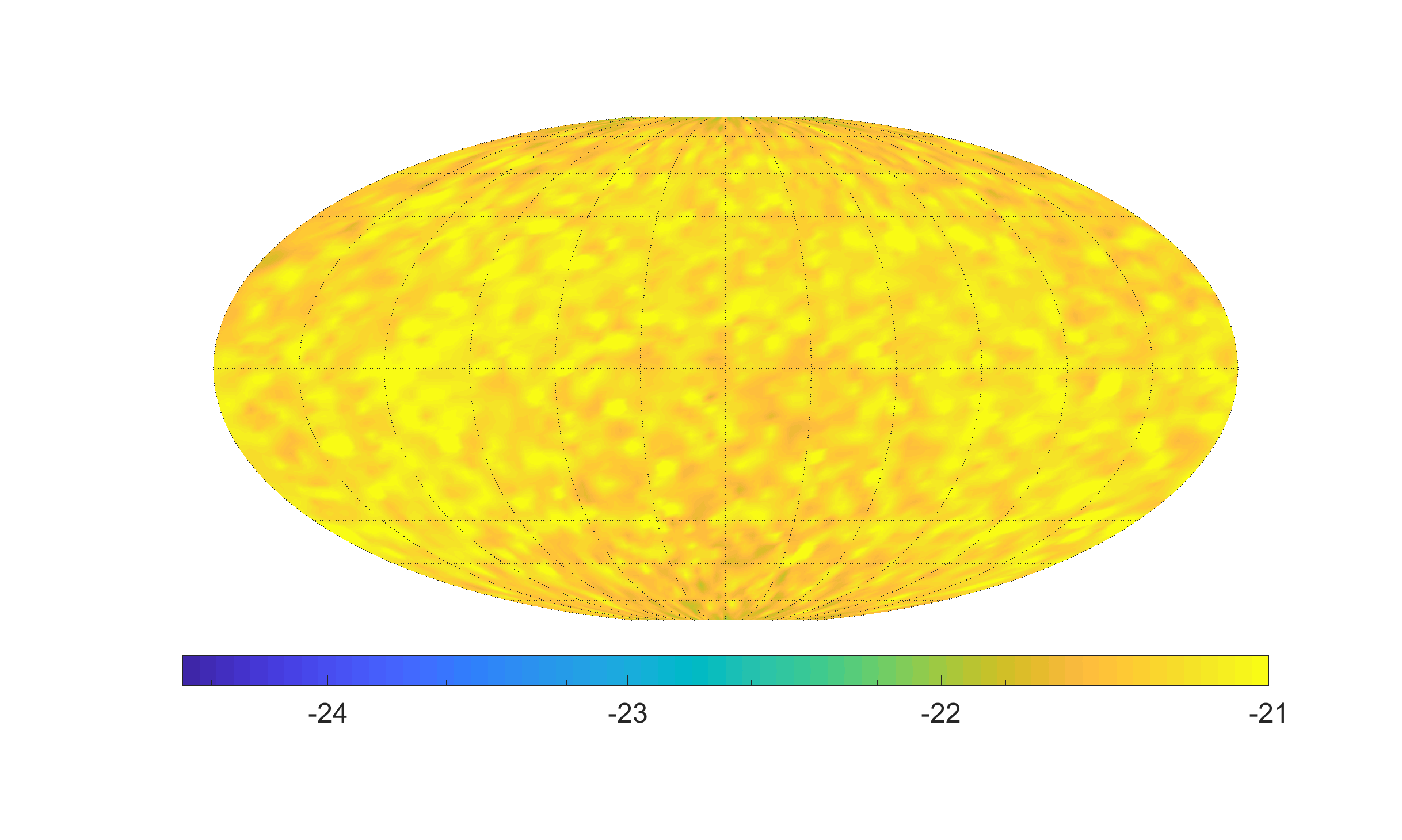
Figure 5: The sky map of amplitude intensity of the WD binary singal at different spatial positions. The horizontal axis represents the longitude ($\lambda\in\left[-\pi,\pi\right]$) and the vertical axis represents the ecliptice latitude ($\beta\in\left[-\pi/2,\pi/2\right]$)

III.3 sky map of WD binaries projected on detectors

(a) $\kappa=0^{\circ}$

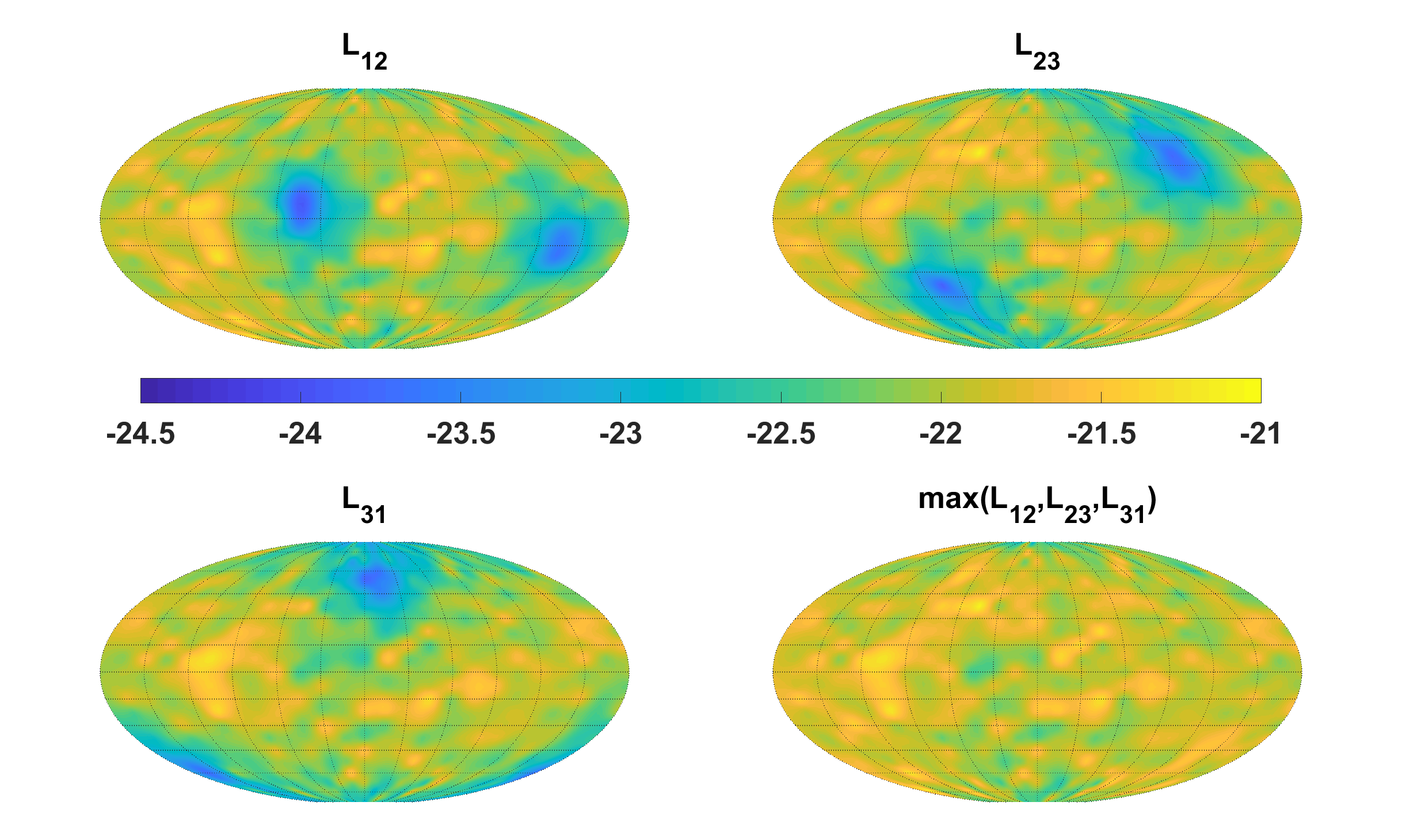
(b) $\kappa=45^{\circ}$

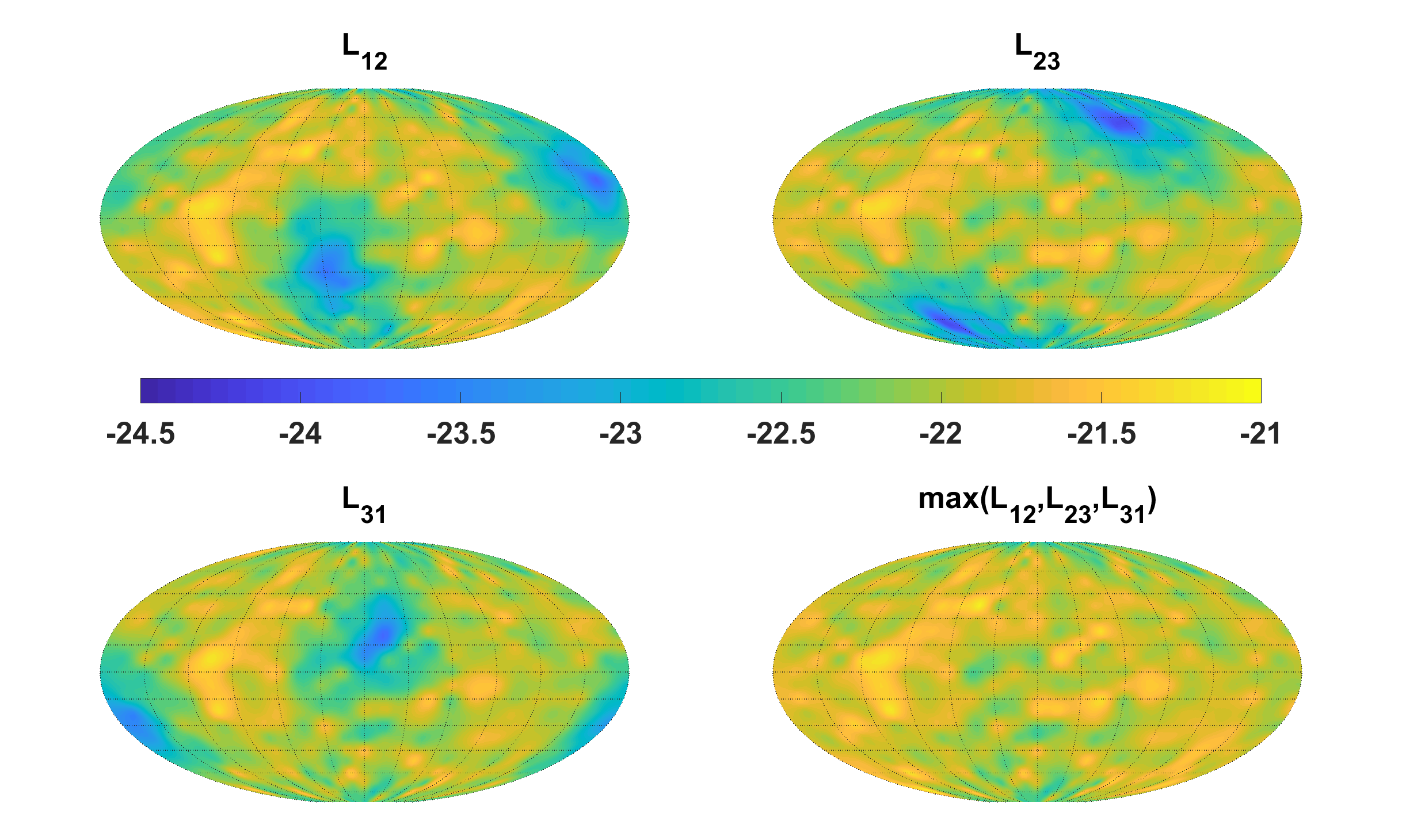
(c) $\kappa=90^{\circ}$

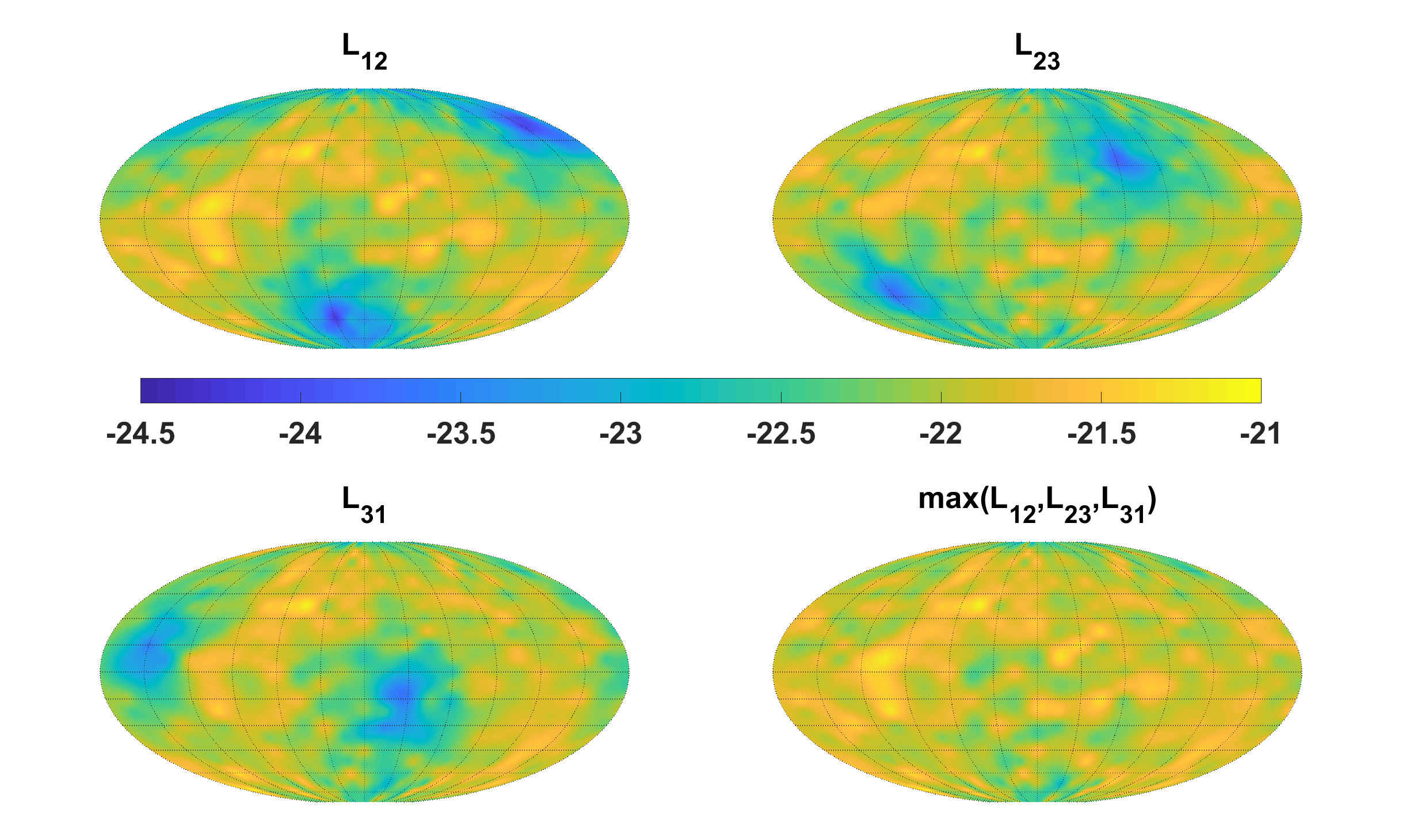
(d) $\kappa=135^{\circ}$

Figure 6: The sky map of amplitude of the source projected on $L_{12}$, $L_{23}$, and $L_{31}$ and the maximum amplitude of the WD binaries projected on $L_{12}$, $L_{23}$, and $L_{31}$ for different variable $\kappa$ respectively. The variable $\kappa$ ($\kappa\in\left[0,2\pi\right]$) is divided into 8 equal parts.

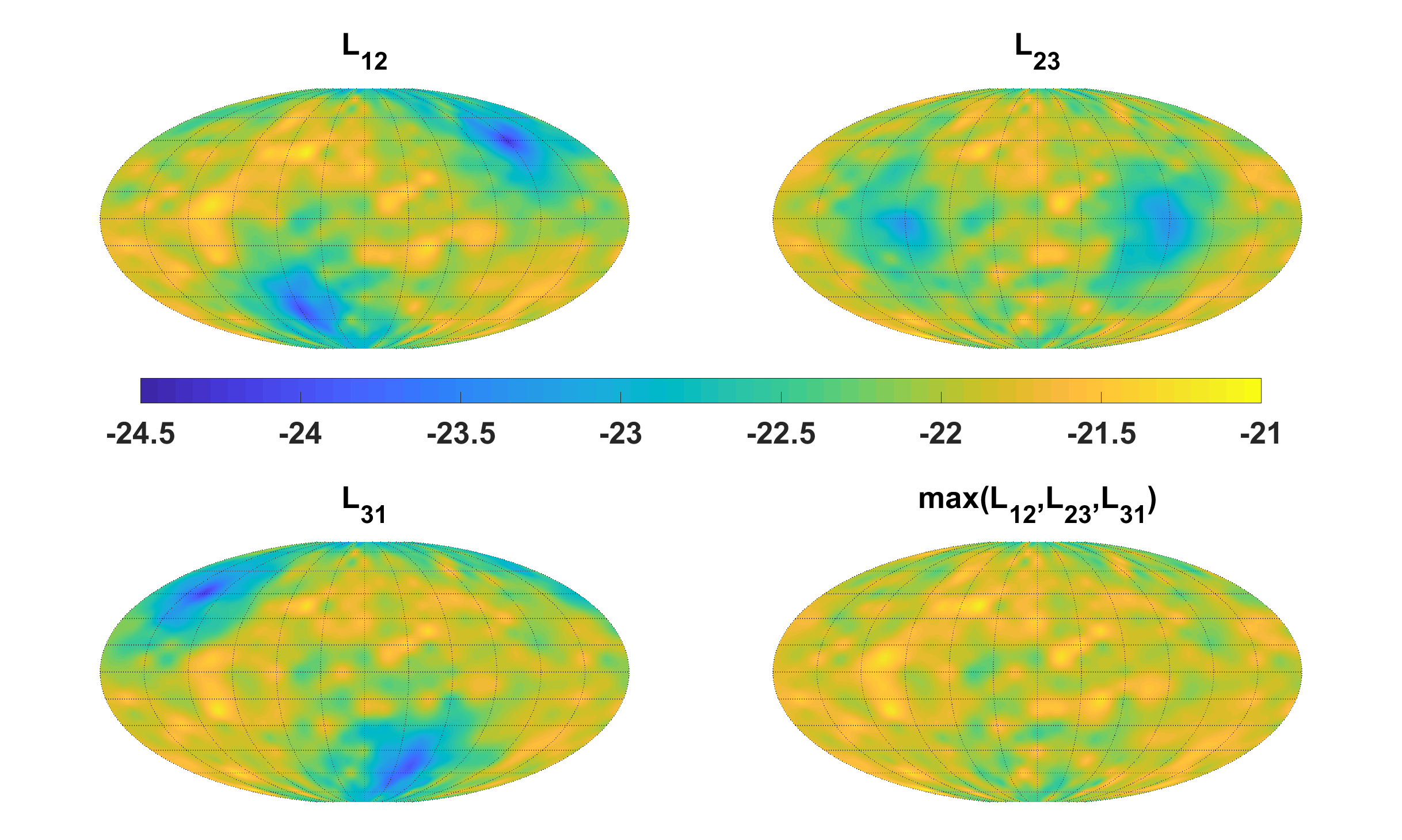
(a) $\kappa=180^{\circ}$

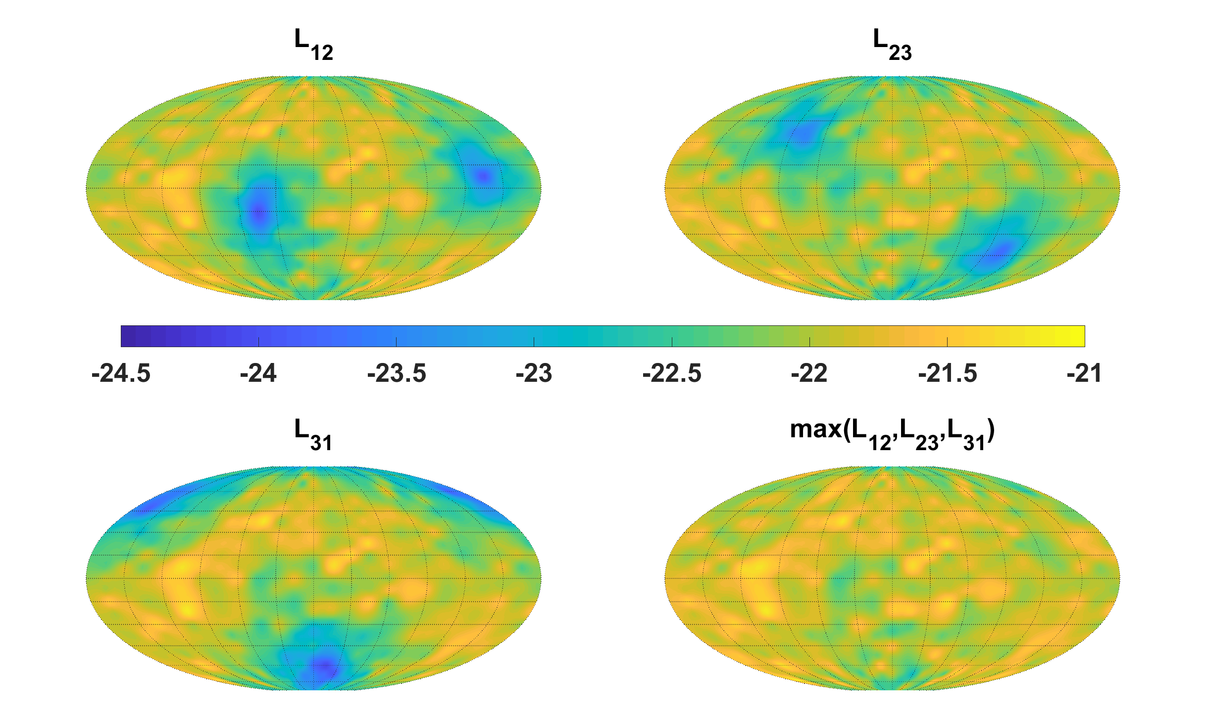
(b) $\kappa=225^{\circ}$

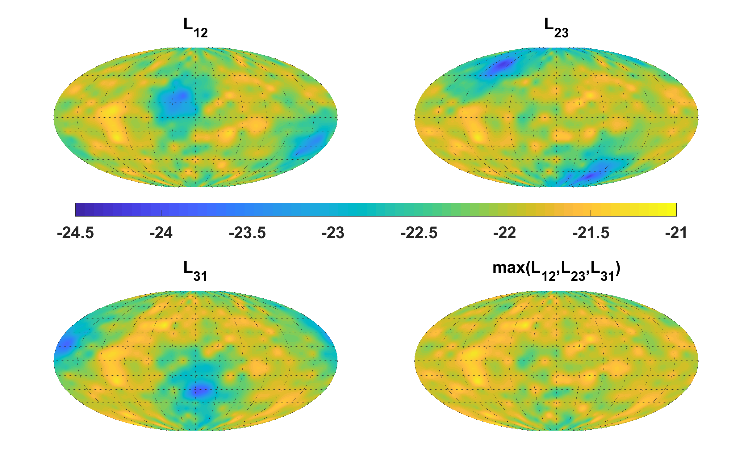
(c) $\kappa=270^{\circ}$

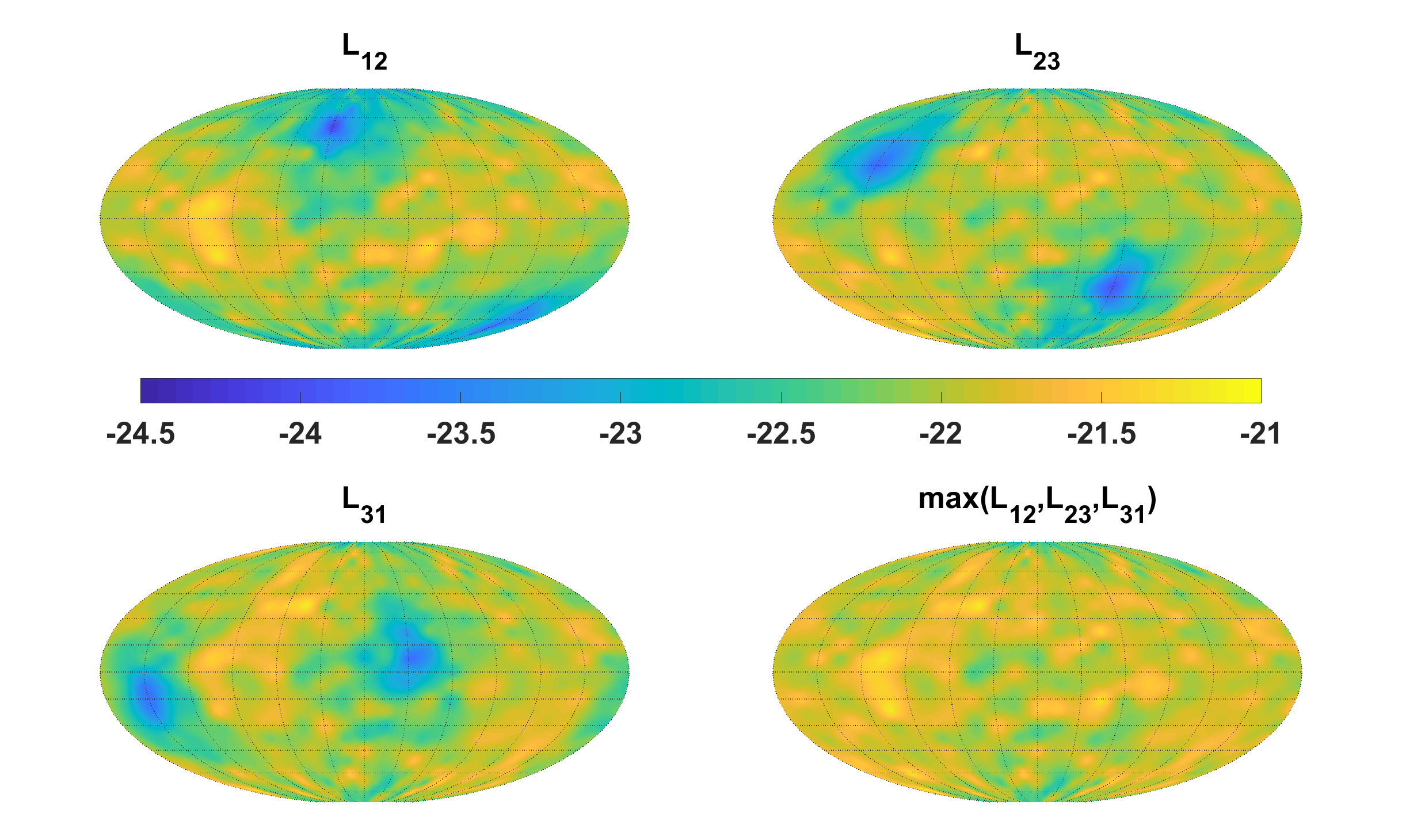
(d) $\kappa=315^{\circ}$

Figure 7: The sky map of amplitude of the source projected on $L_{12},L_{23},L_{31}$ and the maximum amplitude of the WD binaries projected on $L_{12},L_{23}$ and $L_{31}$ for different variable $\kappa$ respectively. The variable $\kappa$ ($\kappa\in\left[0,2\pi\right]$) is divided into 8 equal parts.

For an identified wave source, in order to better observe the effect of different orbital positions of the detectors on its observation data, we just consider the short-time observation of a WD binary. Since its observation time is so small relative to the one-year observation period, the change of amplitude of the projected signal on detectors caused by the the detector motion in the short observation time can be ignored. Here, the amplitude of the projected signal is normalized and represents the maximum value of the projected signal in a period. For the same source and the same short observation time, the different detector positions in a one-year period can get the different amplitude of the projected signal on detectors. In contrast to the section II.3, the variable $\kappa$ ($\kappa\in\left[0,2\pi\right]$) is divided into 8 equal parts and we can get 8 sky maps for amplitude of WD binaries projected on each detection arm. The sky map shows amplitude of WD binaries projected on $L_{12},L_{23},L_{31}$ in the whole space projected on three detection arms respectively. The coordinates under the $SSB$-frame are also composed of the spatial position coordinates ($\beta,\lambda$). In every sky map, the horizontal axis represents the longitude ($\lambda\in\left[-\pi,\pi\right]$) and the vertical axis represents the ecliptice latitude ($\beta\in\left[-\pi/2,\pi/2\right]$). So we can get the grids of $24\times 24$ on the sky map. Then we calculate the amplitude maximum of WD projected signal for each grid on sky map. Here, the parameters of the WD binaries are the same as the one in section III.2 and the detector response is shown in Eq. (9). Here, we choose only the maximum value and keep it as the amplitude maximum value at that spatial location. The sky map of amplitude of the source projected on $L_{12}$, $L_{23}$, and $L_{31}$ and the maximum amplitude of the WD binaries projected on $L_{12},L_{23}$ and $L_{31}$ for different variable $\kappa$ respectively are shown in Fig. 6 and Fig. 7. For a WD binary of the frequency $f_{0}$, the sampling frequency $F_{s}=10\times f_{0}$, the data counts $N=128$. So we can calculate the observation time $T_{OB}=N/F_{s}=1/(12.8\times f_{0})$. For the frequency $f_{0}=10^{-4}Hz$, the observation time $T_{OB}=781.25s$ can be calculated, which is a short-time observation for the one-year period of detector orbit. Due to the different frequencies of WD binary singals, the observation time of each WD binary singal is not the same. However, the amplitude value does not change due to the difference in the number of observation signal periods caused by the slight difference in the short observation time.

Next, we discuss the effect of observation time on the amplitude of the projected signals. We select 4 verification binaries signals: J0806, V407 Vul, ES Cet, SDSSJ1351, whose parameters are detailed in Kupfer et al. (2018). The polarisation angle is set $\psi=0$, and initial orbital phase is set $\phi_{0}=0$. Then we can calculate the amplitudes of the projected signals on the three detection arms $L_{12}$, $L_{23}$, and $L_{31}$, respectively, and obtain the results of the joint observation of the three detection arms. We selected 4 different observation time $T_{OB}=N\times f_{0}$. Where $f_{0}$ is the frequency of VB signal and N is the number of the VB cycles observed during the observation time. We set $N=10,100,1000,10000$. The amplitude of projection signals of four VB signals at different observation time are shown in Fig. 8. From the Fig. 8, we can find that the amplitude difference is not significant at $N=10,100,1000$. However, the amplitude is significantly different at $N=10000$.

In the Fig. 9, we give the variation range of the characteristic strain $h_{c}$ of the 4 VB signals for all $L_{{ij},\kappa}$ for TAIJI (The 4 color error bars correspond to 4 different observation times and N is the number of the VB cycles observed during the observation time) compared with the noise amplitude $h_{n}$ of TAIJI (red line) and LISA (blue line). Here, the characteristic strain $h_{c}=\sqrt{N}\times A$, the noise amplitude $h_{n}=\sqrt{f\times S_{n}(f)}$.

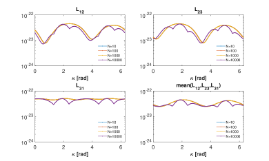
(a) VB: J0806

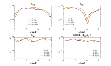
(b) VB: V407 Vul

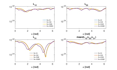
(c) VB: ES Cet

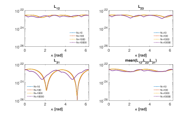
(d) VB: SDSSJ1351

Figure 8: The amplitude of projection signals of four VB signals at different observation time. N is the number of the VB cycles observed during the observation time.

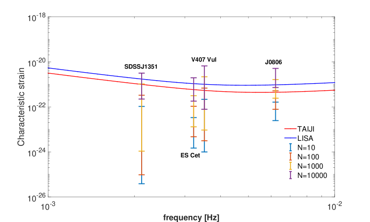
Figure 9: The variation range of the characteristic strain $h_{c}$ of the 4 VBs for all $L_{{ij},\kappa}$ for TAIJI (The 4 color error bars correspond to 4 different observation times and N is the number of the VB cycles observed during the observation time) compared with the noise amplitude $h_{n}$ of TAIJI (red line) and LISA (blue line).

IV Localizing the sky position of identified WD binary

Due to the periodic orbit motion of the detector, the results of short time observation are related to the orbit position of the detector. For some specific WD binary sources, the best localizing the sky position of the sources at the best detector position is achieved.

Here, we select 4 verification binaries signals: J0806, V407 Vul, ES Cet, SDSSJ1351 as the identified sources, whose parameters are detailed in Kupfer et al. (2018). The polarisation angle is set $\psi=0$, and initial orbital phase is set $\phi_{0}=0$. The sky location parameters ($\lambda[rad],sin\beta,D_{L}[kpc]$) of 4 VB signals are set as: (2.1021, -0.0820, 5), (5.1486, 0.7288, 1.786), (0.4295, -0.3475, 1.584), (3.6370, 0.0780, 1.317), respectively. The posterior distribution lies typically in a small volume of the parameter space. The research on localizing the sky position of identified WD binary based on short-term period observation is mainly divided into 3 steps:

Step 1: Find the reduced parameter space as the new prior. Estimate $1\sigma$ of the sky position parameters using the Fisher Information Matrix and frame the $3\sigma$ covariance region centered on the true value of the parameter as the reduced parameter space for the next steps.

Step 2: Find best orbit position of detector. For each VB source, find best orbit position of detector with the smallest parameter error.

Step 3: Get the posterior. Use Metropolis-Hastings MCMC to get the posterior distribution of the location parameters at the best orbit position of detector.

In this paper, the detector response form in the time domain is used, so we will get the gravitational wave data in the time domain. When calculating the likelihood for each samples, we convert the data in time domain into frequency-domain through FFT. For a WD binary of the frequency $f_{0}$, the sampling frequency $F_{s}=10\times f_{0}$, the data counts $N=128$. So we can calculate the observation time $T_{OB}=N/F_{s}=1/(12.8\times f_{0})$. Detailed calculation and related theories are shown below.

IV.1 Bayesian inference

The Bayesian inference is based on calculating the posterior probability distribution function (PDF) of the unknown parameter set $\bm{\theta}=\{\theta_{1},\dots,\theta_{m}\}$ in a given model, which actually updates our state of belief from the prior PDF of $\bm{\theta}$ after taking into account the information provided by the experimental data set $D$. The posterior PDF is related to the prior PDF by the Bayes’s therom

$$p(\bm{\theta}|D)=\frac{\mathcal{L}(D|\bm{\theta})\pi(\bm{\theta})}{p(D)},$$ (20)

where $\mathcal{L}(D|\bm{\theta})$ is the likelihood function, and $\pi(\bm{\theta})$ is the prior PDF which encompasses our state of knowledge on the values of the parameters before the observation of the data. The quantity $p(D)$ is the Bayesian evidence which is obtained by integrating the product of the likelihood and the prior over the whole volume of the parameter space

$$p(D)=\int_{V}\mathcal{L}(D|\theta)\pi(\bm{\theta})d\theta.$$ (21)

The evidence is an important quantity for Bayesian model comparison.It is straight forward to obtain the marginal PDFs of interested parameters $\{\theta_{1},\dots,\theta_{n}\}(n<m)$ by integrating out other nuisance parameters $\{\theta_{n+1},\dots,\theta_{m}\}$

$$p(\theta_{1},\dots,\theta_{n})_{\text{marg}}=\int p(\bm{\theta}|D)\prod_{i=n+1}^{m}d\theta_{i}.$$ (22)

The marginal PDF is often used in visual presentation. If there is no preferred value of $\theta_{i}$ in the allowed range ($\theta_{i,\text{min}}$, $\theta_{i,\text{max}}$), the priors can be taken as a flat distribution

$$\pi(\theta_{i})\propto\left\{\begin{tabular}[]{ll}1,&\text{for } $\theta_{i,\text{min}}<\theta_{i}<\theta_{i,\text{max}}$\\ 0,&\text{otherwise}\end{tabular}\right..$$ (25)

The likelihood function is often assumed to be Gaussian

$$\mathcal{L}(D|\bm{\theta})=\prod_{i}\frac{1}{\sqrt{2\pi\sigma_{i}^{2}}}\exp\left[-\frac{(f_{\text{th},i}(\bm{\theta})-f_{\text{exp},i})^{2}}{2\sigma_{i}^{2}}\right],$$ (26)

where $f_{\text{th},i}(\bm{\theta})$ are the predicted $i$-th observable from the model which depends on the parameter set $\bm{\theta}$, and $f_{\text{exp},i}$ are the ones measured by the experiment with uncertainty $\sigma_{i}$. For experiments with only a few events observed, the form of the likelihood function can be taken as Poisson. When the form of the likelihood function is specified, the posterior PDF can be determined by sampling the distribution according to the prior PDF and the likelihood function using Markov Chain Monte Carlo (MCMC) methods. The statistic mean value of a parameter $\theta$ can be obtained from the posterior PDF $P(\bm{\theta}|D)$ in a straight forward manner. Using the MCMC sequence $\{\theta^{(1)}_{i},\theta^{(2)}_{i},\dots,\theta^{(N)}_{i}\}$ of the parameter $\theta_{i}$ with $N$ the length of the Markov chain, the mean (expectation) value $\langle\theta_{i}\rangle$ is given by

$$\langle\theta_{i}\rangle=\int\theta_{i}P(\theta_{i}|D)d\theta_{i}=\frac{1}{N}\sum_{k=1}^{N}\theta^{(k)}_{i}.$$ (27)

The $1\sigma$ standard deviation of the parameter $\theta_{i}$ is given by $\sigma^{2}=\sum^{N}_{k=1}(\theta^{(k)}_{i}-\langle\theta_{i}\rangle)^{2}/(N-1)$.

IV.2 Fisher Information Matrix

The Fisher Information Matrix (FIM) is a popular choice to estimate the parameter uncertainty for GW signals. Here, we choose joint observations of the detector $arm12$, $arm23$ and $arm31$ to calculate the FIM

$$F_{ij}=F_{ij}^{12}+F_{ij}^{23}+F_{ij}^{31}$$ (28)

$$F_{ij}^{lk}=\left\langle\frac{\partial h_{lk}}{\partial\theta^{i}}\bigg{|}\frac{\partial h_{l}k}{\partial\theta^{j}}\right\rangle$$ (29)

where $h_{lk}$ is the response of the detector $arm_{lk}$ to a gravitational wave signal and $\theta^{i}$ is $i_{th}$ component of the sky position parameters of the signal, $\{\lambda,sin\beta,D_{L}\}$.

The instrument noise of detector was ignored, and we focus on the projected signal on the single arm detector of an identified WD binary. In this paper, $h_{lk}$ are the ones measured by the experiment with uncertainty $\sigma=a\times h_{lk}$. So the noise is set as the Gaussian noise with mean $\mu=0$, standard deviation $\sigma=a\times h_{lk}$. For SNR=7, we can get $a=0.3578$.

The matrix inversion of the FIM gives the Gaussian covariance matrix, $F_{ij}^{-1}=C_{ij}$. To estimate the position of the WD binary in the sky, following Cutler (1998), the solid angle

$$\Delta\Omega_{s}=2\pi\cos{\beta}\sqrt{C_{\beta\beta}C_{\lambda\lambda}-C_{\beta\lambda}^{2}}$$ (30)

where

$$C_{\beta\beta} = C_{sin\beta sin\beta}\times\cos{\beta_{0}}^{2}$$

$$C_{\beta\lambda} = C_{sin\beta\lambda}\times\cos{\beta_{0}}$$ (31)

where $\beta_{0}$ is the real value of the parameter $\beta$ of the identified WD binary.

IV.3 best and worst orbit position for observation

For an identified wave source, in order to better observe the effect of different orbital positions of the detectors on its observation data, we just consider the short-time observation of a WD binary. In this case, the variable, the initial ecliptic longitude $\kappa$ in detector orbit, is selected to present the detector position.

Take 12 different $\kappa$ values uniformly in the interval $\kappa\in\left[0,2\pi\right]$. Then we can get the $1\sigma$ of the sky position parameters using the Fisher Information Matrix for different $\kappa$ values for each VB source. The solid angle and $\Delta D_{L}/D_{L}$ at different $\kappa$ values for each VB sources are caculated. So the solid angle and $\Delta D_{L}/D_{L}$ can be effected by the orbit position. But the difference of $\Delta D_{L}/D_{L}$ is much smaller than the difference of the solid angle at different orbit position. Here we select the value of the solid angle as the criterion for judging the best and worst observations. Then take 365 different $\kappa$ values uniformly in the interval $\kappa\in\left[0,2\pi\right]$ and find the best and worst orbit position $\kappa$ and the $1\sigma$ of the sky position parameters. Frame the $3\sigma$ covariance region as the reduced parameter space, which was set as the prior. The details are shown in the Tab. 1. The numbers in red color were replaced by the bounds on the sky position parameters of WD, because the numbers calculated by FIM were out of bounds. The reduced parameter space of sky position parameters at best $\kappa$ was appropriately expanded because the $3\sigma$ covariance region was too small.

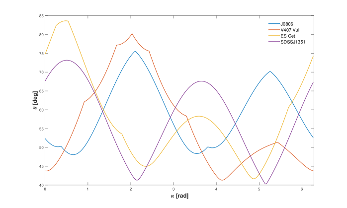
Figure 10: The relationship between the orbital position $\kappa$ and the mean of the Angle $\theta$ of $L_{12,\kappa}$, $L_{23,\kappa}$ and $L_{31,\kappa}$ for J0806, V407 Vul, ES Cet, SDSSJ1351,respectively.

Table 1: The prior calculated by FIM at best and worst obit position. The numbers in red color were replaced by the bounds on the sky position parameters of WD, because the numbers calculated by FIM were out of bounds.

$\mathbf{VB}$	$\mathbf{orbit\ position}$	$\mathbf{\lambda[rad]}$	$\mathbf{sin\beta}$	$\mathbf{D_{L}[kpc]}$
$\mathbf{J0806}$	best ($\kappa=0.67135$)	[2.0870,2.1171]	[-0.15290,-0.01110]	[1.7362,8.2637]
	worst ($\kappa=5.2675$)	[-0.5179,4.7221]	[-0.2270,0.0630]	[0.9931,9.0069]
$\mathbf{V407Vul}$	best ($\kappa=1.3599$)	[5.1297,5.1675]	[0.71105,0.74647]	[0.62869,2.9433]
	worst ($\kappa=3.1502$)	[4.4669,5.8303]	[-0.5057,1.0]	[0.003,4.0017]
$\mathbf{ESCet}$	best ($\kappa=4.5273$)	[0.35000,0.5091]	[-0.38334,-0.31163]	[0.33445,2.8335]
	worst ($\kappa=0.2926$)	[-3.14,3.14]	[-1.0,1.0]	[0.5950,2.5730]
$\mathbf{SDSSJ1351}$	best ($\kappa=1.5837$)	[3.5066, 3.7674]	[-0.08063, 0.23657]	[0.40787, 2.2261]
	worst ($\kappa=3.6838$)	[0.7638, 6.28]	[-1.0, 1.0]	[0.003, 3.3580]

IV.4 Posterior

Sky location parameter is set by $\bm{\theta}=\{\lambda,sin\beta,D_{L}\}$. The reduced parameter space as new prior was obtained at best and worst orbit position. The reduced parameter space can be used to set the desired parameter boundaries as the new prior. $136000$ samples of one MCMC chain were selected and then Metropolis-Hastings sampling was used to obtain the posterior distribution of parameters. When calculating the likelihood for each MCMC samples, the experiment with uncertainty $\sigma_{i}$ is chosen to be $\sigma_{i}=0.3578\times f_{\text{exp},i}$ and $\chi^{2}=\chi_{arm12}^{2}+\chi_{arm23}^{2}+\chi_{arm31}^{2}$ .

The contract of posterior distribution of the sky position parameters ($\lambda,sin\beta,D_{L}$) at best and worst orbit position of 4 VB signals : J0806, V407 Vul, ES Cet and SDSSJ1351 is shown in the Fig. 11, Fig. 12,Fig. 13 and Fig. 14, respectively. We showed one-dimensional and two-dimensional marginalized posterior PDFs of the sky position parameters ($\lambda,sin\beta,D_{L}$) of 4 VB signals with the best-fit value and statistic mean value. The contours enclose the $68\%$ and $95\%$ probability regions of the parameter estimation.

According to the posterior, we find the distribution was not a standard Gaussian. So the result calculated by FIM can be not accurate. Our method gives a much more accurate result. Comparing the observations of the best and worst orbital positions simultaneously, we find that the accuracy of the parameters obtained in the best position is significantly several times higher than that in the worst position.

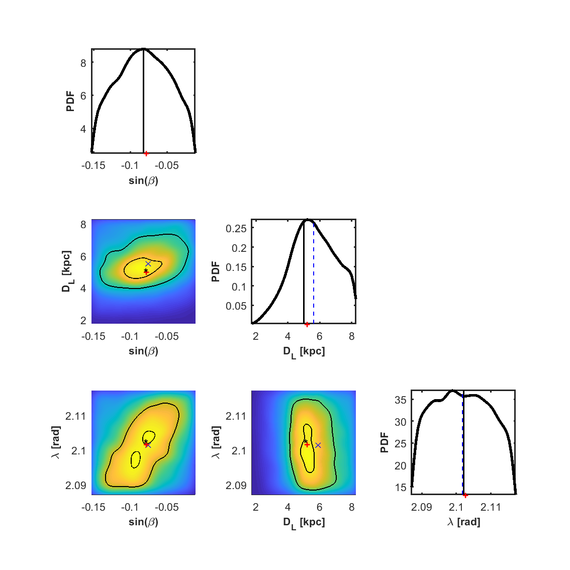
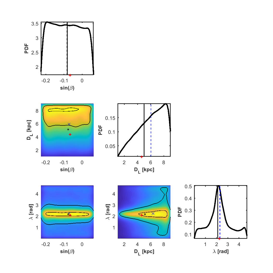
Figure 11: The contract of posterior distribution of the sky position parameters ($\lambda,sin\beta,D_{L}$) at best and worst orbit position of J0806 for TAIJI. The black (blue) vertical line in each one-dimensional marginalized posterior PDFs indicates the true value (statistic mean value). The black star (blue cross) in each two-dimensional marginalized posterior PDFs indicates the true value (statistic mean value). The red plus in each one-dimensional and two-dimensional marginalized posterior PDFs indicates best-fit value. The contours enclose the $68\%$and $95\%$ probability regions of the parameter estimation.

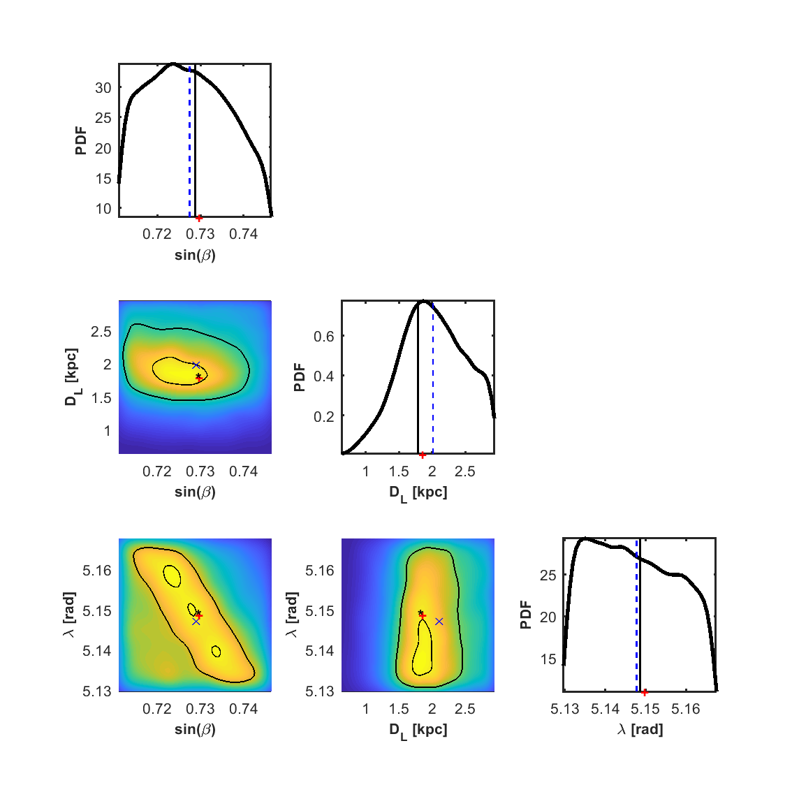
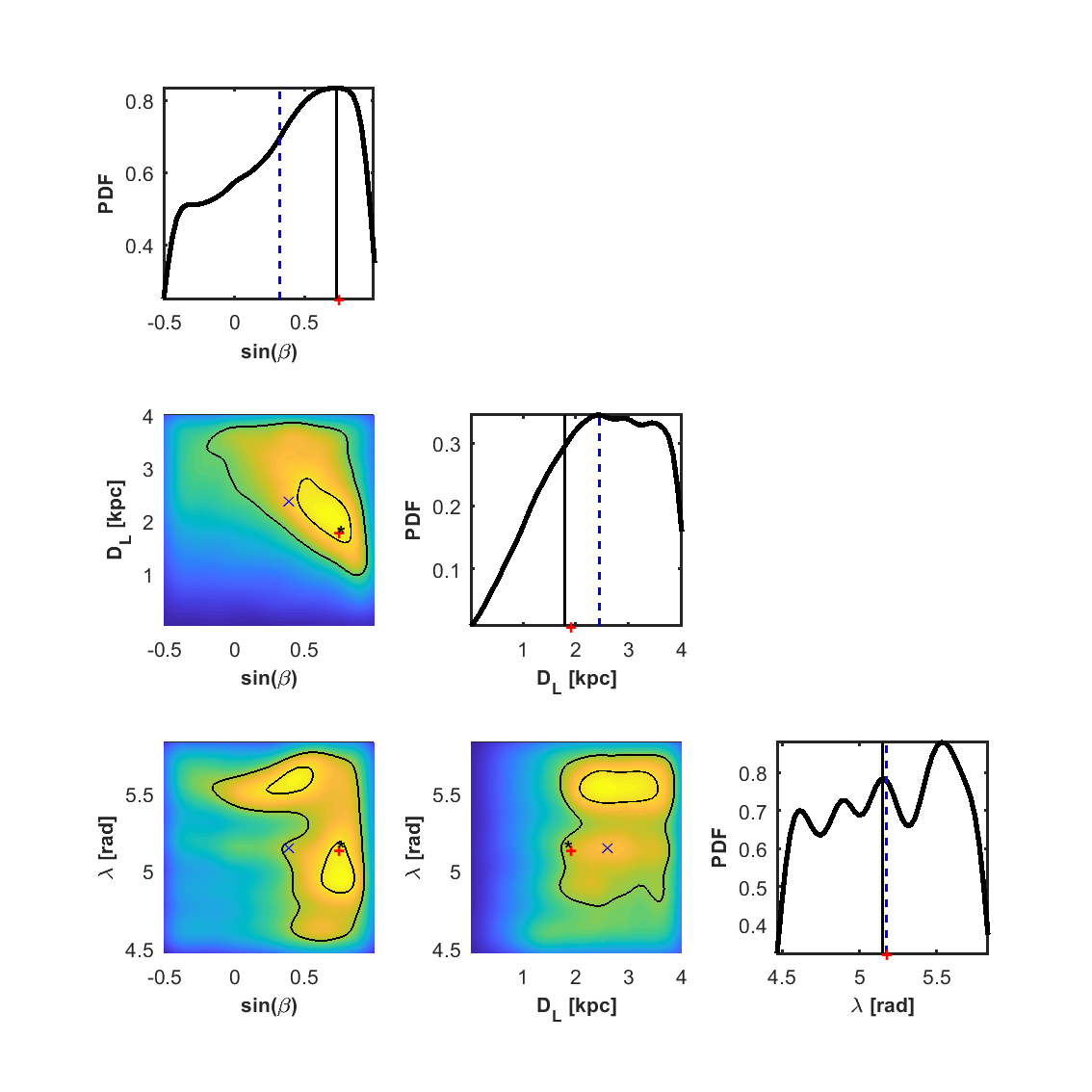
Figure 12: The contract of posterior distribution of the sky position parameters ($\lambda,sin\beta,D_{L}$) at best and worst orbit position of V407 Vul for TAIJI. The black (blue) vertical line in each one-dimensional marginalized posterior PDFs indicates the true value (statistic mean value). The black star (blue cross) in each two-dimensional marginalized posterior PDFs indicates the true value (statistic mean value). The red plus in each one-dimensional and two-dimensional marginalized posterior PDFs indicates best-fit value. The contours enclose the $68\%$and $95\%$ probability regions of the parameter estimation.

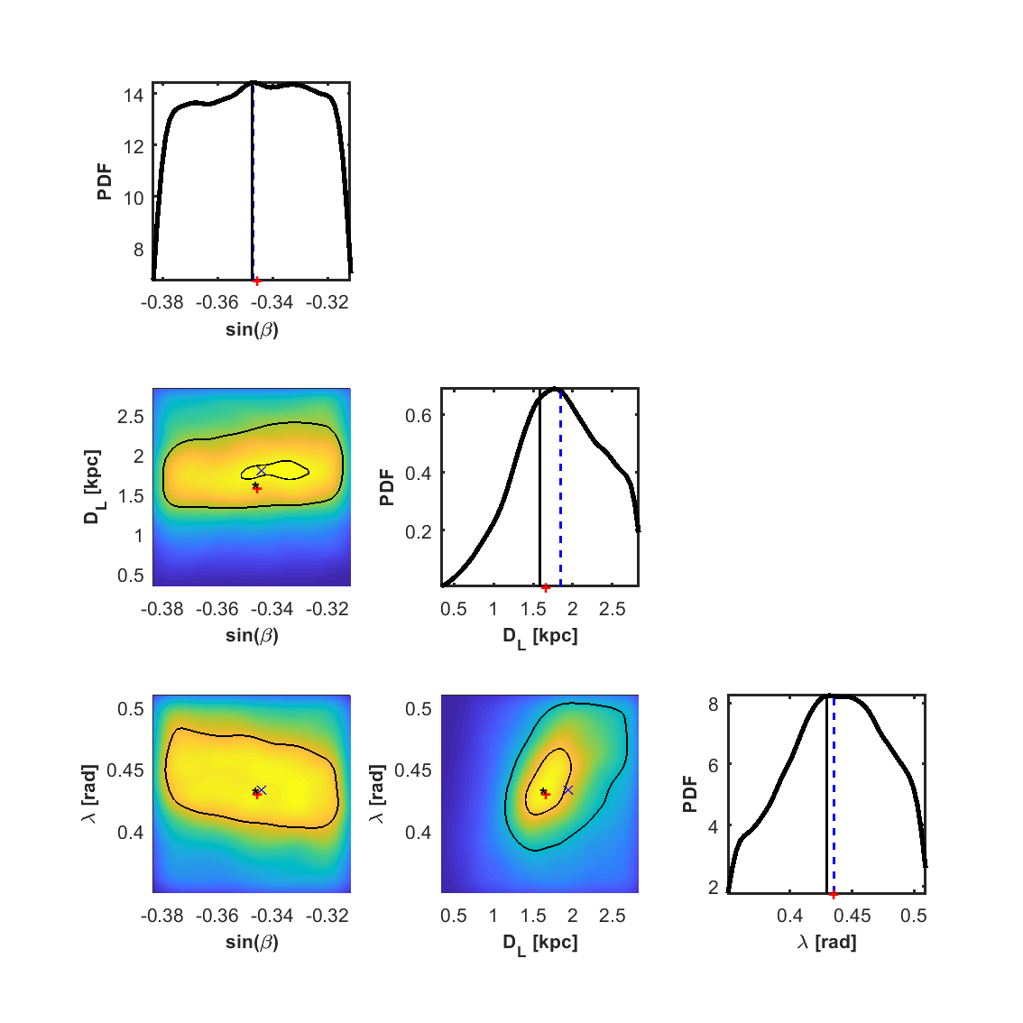
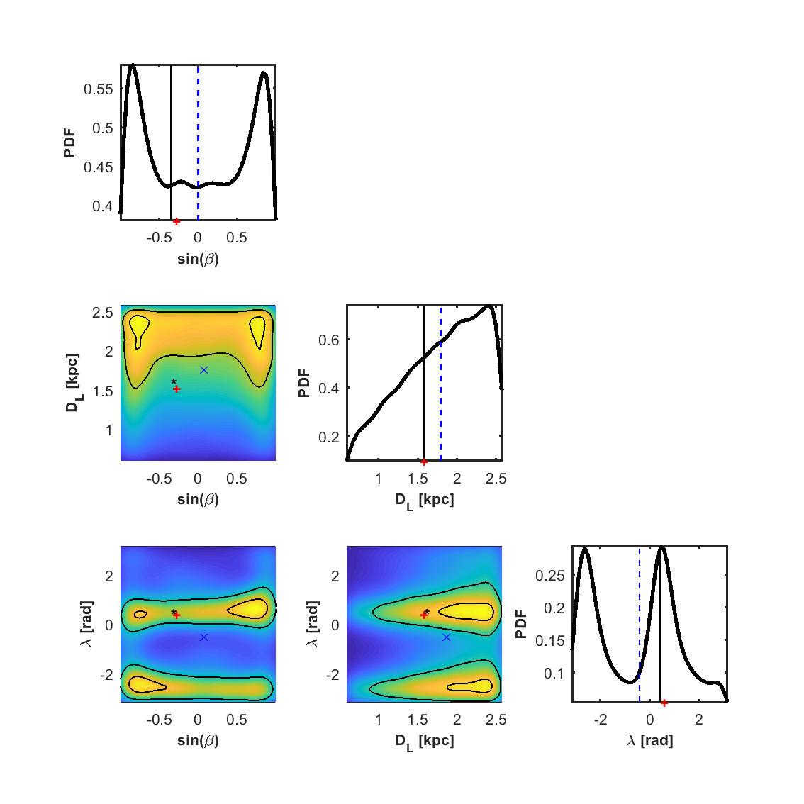
Figure 13: The contract of posterior distribution of the sky position parameters ($\lambda,sin\beta,D_{L}$) at best and worst orbit position of ES Cet for TAIJI. The black (blue) vertical line in each one-dimensional marginalized posterior PDFs indicates the true value (statistic mean value). The black star (blue cross) in each two-dimensional marginalized posterior PDFs indicates the true value (statistic mean value). The red plus in each one-dimensional and two-dimensional marginalized posterior PDFs indicates best-fit value. The contours enclose the $68\%$and $95\%$ probability regions of the parameter estimation.

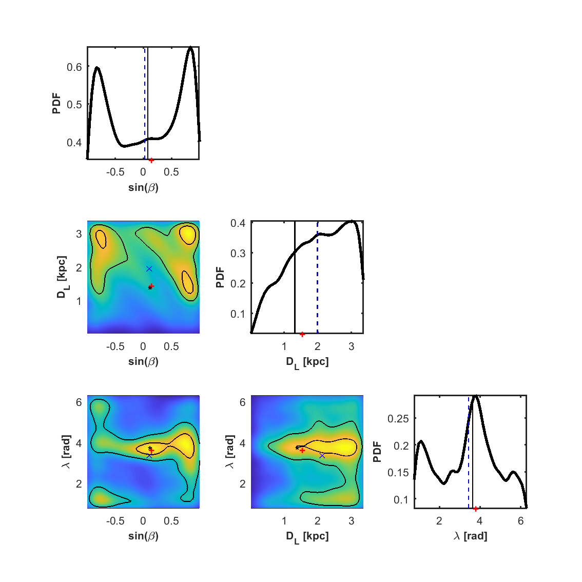
Figure 14: The contract of posterior distribution of the sky position parameters ($\lambda,sin\beta,D_{L}$) at best and worst orbit position of SDSSJ1351 for TAIJI. The black (blue) vertical line in each one-dimensional marginalized posterior PDFs indicates the true value (statistic mean value). The black star (blue cross) in each two-dimensional marginalized posterior PDFs indicates the true value (statistic mean value). The red plus in each one-dimensional and two-dimensional marginalized posterior PDFs indicates best-fit value. The contours enclose the $68\%$and $95\%$ probability regions of the parameter estimation.

IV.5 LISA-TAIJI network

(a) VB : J0806.

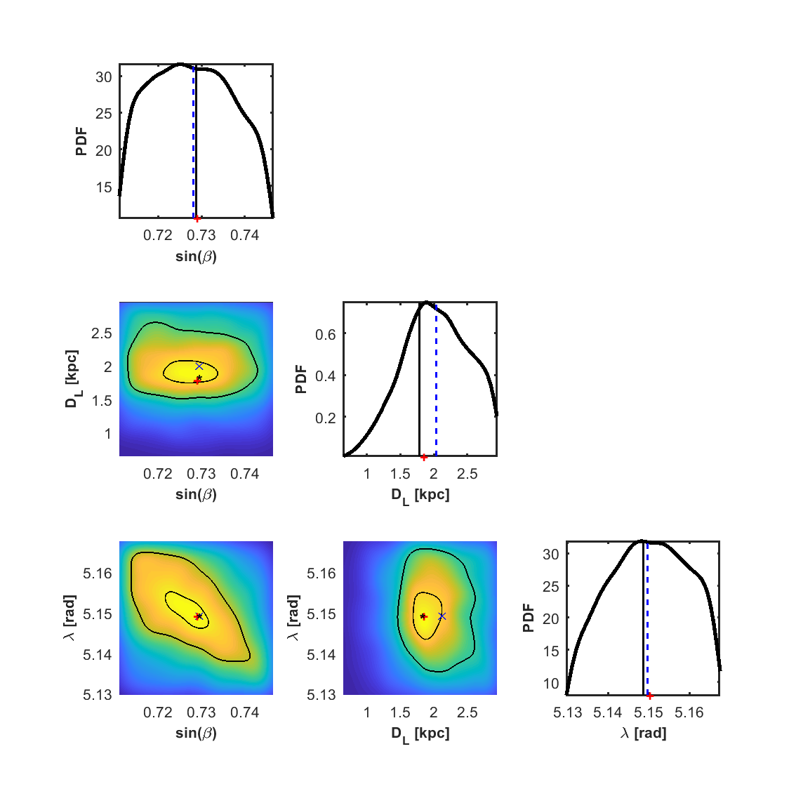
(b) VB : V407 Vul.

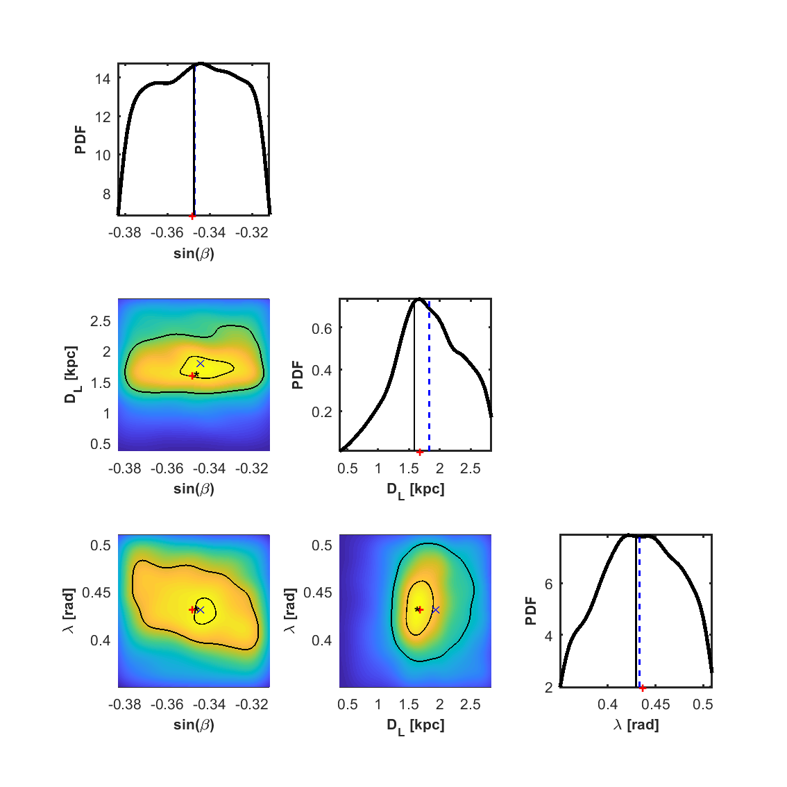
(c) VB : ES Cet.

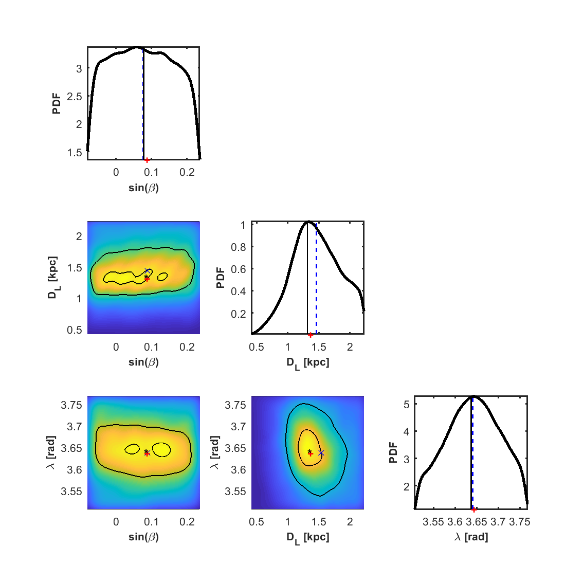
(d) VB : SDSSJ1351.

Figure 15: TAIJI-LISA network: Posterior distribution of the sky position parameters ($\lambda,sin\beta,D_{L}$) of 4 VB signals : J0806, V407 Vul, ES Cet, SDSSJ1351, respectively. The black (blue) vertical line in each one-dimensional marginalized posterior PDFs indicates the true value (statistic mean value). The black star (blue cross) in each two-dimensional marginalized posterior PDFs indicates the true value (statistic mean value). The red plus in each one-dimensional and two-dimensional marginalized posterior PDFs indicates best-fit value. The contours enclose the $68\%$and $95\%$ probability regions of the parameter estimation.

Now we discuss the sky localization estimations of TAIJI-LISA network. When we choose the arm length $L_{TAIJI}=3\times 10^{9}m$ and the orbit location variable $\kappa_{TAIJI}$ for TAIJI, we choose the arm length $L_{LISA}=2.5\times 10^{9}m$ and the orbit location variable $\kappa_{LISA}=\kappa_{TAIJI}-40\pi/180$. We selected the best orbit position to get the posterior distribution of the sky position parameters ($\lambda,sin\beta,D_{L}$) of 4 VB signals : J0806, V407 Vul, ES Cet, SDSSJ1351. Here, when calculating the likelihood for each MCMC samples, the experiment with uncertainty $\sigma_{i}$ is also chosen to be $\sigma_{i}=0.3578\times f_{\text{exp},i}$ and $\chi^{2}=\chi_{TAIJI}^{2}+\chi_{LISA}^{2}$.Here, $\chi_{TAIJI}^{2}=\chi_{arm12_{TAIJI}}^{2}+\chi_{arm23_{TAIJI}}^{2}+\chi_{arm31_{TAIJI}}^{2}$ , $\chi_{LISA}^{2}=\chi_{arm12_{LISA}}^{2}+\chi_{arm23_{LISA}}^{2}+\chi_{arm31_{LISA}}^{2}$.

The posterior distribution of the sky position parameters ($\lambda,sin\beta,D_{L}$) of 4 VB signals : J0806, V407 Vul, ES Cet, SDSSJ1351, respectively is shown in the Fig. 15. The priors were selected as the same as the Tab. 1 at best orbit position of the TAIJI. We showed one-dimensional and two-dimensional marginalized posterior PDFs of the sky position parameters ($\lambda,sin\beta,D_{L}$) of 4 VB signals with the best-fit value and statistic mean value. The contours enclose the $68\%$and $95\%$ probability regions of the parameter estimation.

By Comparison between Fig. 15 and the four figures above for J0806, V407 Vul, ES Cet and SDSSJ1351, the network of two detectors does not significantly improve the accuracy of location of the verification binaries. The reason of that result is that one GW source can not be perpendicular to both detectors of TAIJI and LISA for a short observation time. For a long observation time, the network of two detectors has a significant improvement to angular resolution.

V Conclusion and Discussion

In this paper, we focus on localizing the sky position of gravitational wave source for the identified white dwarf binaries. For the first time, the influence of the periodic orbit position parameter $\kappa$ of space-based laser interferometer detectors on the localizing the sky position of the identified double white dwarf binaries is considered in this paper.

We present the sky maps of the WD binaries in the Milky Way before and after the projection on the detectors. The results show that $(1)$ the intensity distribution of the WD binaries is not uniform in the whole space ; $(2)$ different detector positions have a modulation effect on the detector response of the same WD binaries source; $(3)$ the amplitude modulation effect of a single detection arm on the WD binaries in the whole space presents a symmetrical effect in the sky position ($\lambda,\beta$) and the sky position ($\lambda+\pi,-\beta$); $(4)$ Joint observations of three detectors on the same WD binaries can significantly improve the situation that the amplitude of the source decreases significantly on a single detection arm.

Due to the periodic orbit motion of the detector, the results of short-term observation are related to the orbit position of the detector. We select best orbit position to realize the joint observations on the three detection arms for the 4 verification binaries(VB). Firstly, the new prior framed the $3\sigma$ covariance region centered on the true value of the parameters was calculated by FIM and then find the best orbit position for observation. Finally, the posterior can be estimated using the Metropolis-Hastings MCMC method. Comparing the observations of the best and worst orbital positions simultaneously, we find that the accuracy of the parameters obtained in the best position is significantly several times higher than that in the worst position. The posterior distribution of the sky position parameters of the 4 VB sources are gotten based on TAIJI and LISA network. Compared with a single detector, the network of two detectors does not significantly improve the accuracy of location of the verification binaries. The reason of that result is that one GW source can not be perpendicular to both detectors of TAIJI and LISA for a short observation time. For a long observation time, the network of two detectors has a significant improvement to angular resolution.

Space-based gravitational wave detection, such as LISA and TAIJI, will actually be able to observe space gravitational waves in the 2030s. This paper will provide a more rapid and accurate localization the sky position of identified sources.

References

- The LIGO Scientific Collaboration et al. (2021) The LIGO Scientific Collaboration, the Virgo Collaboration, and the KAGRA Collaboration (2021), eprint 2111.03606, URL http://arxiv.org/abs/2111.03606.
- Abbott et al. (2023) R. Abbott, H. Abe, F. Acernese, K. Ackley, S. Adhicary, N. Adhikari, R. X. Adhikari, V. K. Adkins, V. B. Adya, C. Affeldt, et al., The Astrophysical Journal Supplement Series 267, 29 (2023), ISSN 0067-0049, eprint 2302.03676, URL https://iopscience.iop.org/article/10.3847/1538-4365/acdc9f.
- Ruan et al. (2020a) W.-H. Ruan, C. Liu, Z.-K. Guo, Y.-L. Wu, and R.-G. Cai, Nature Astronomy 4, 108 (2020a), ISSN 2397-3366, eprint 2002.03603, URL http://www.nature.com/articles/s41550-019-1008-4.
- Baker et al. (2007) J. Baker, E. Barausse, P. Bender, D. Bortoluzzi, and J. Camp, Van Nostrand’s Scientific Encyclopedia (2007).
- Amaro-Seoane et al. (2017) P. Amaro-Seoane, H. Audley, S. Babak, J. Baker, E. Barausse, P. Bender, E. Berti, P. Binetruy, M. Born, D. Bortoluzzi, et al. (2017), eprint 1702.00786, URL http://arxiv.org/abs/1702.00786.
- Hu and Wu (2017) W.-R. Hu and Y.-L. Wu, National Science Review 4, 685 (2017), ISSN 2095-5138.
- Allen and Ottewill (1997) B. Allen and A. C. Ottewill, Physical Review D 56, 545 (1997), ISSN 0556-2821, eprint 9607068, URL https://link.aps.org/doi/10.1103/PhysRevD.56.545.
- Cornish (2001) N. J. Cornish, Classical and Quantum Gravity 18, 4277 (2001), ISSN 0264-9381, eprint 0105374, URL https://iopscience.iop.org/article/10.1088/0264-9381/18/20/307.
- Cornish and Rubbo (2003) N. J. Cornish and L. J. Rubbo, Physical Review D 67, 029905 (2003), ISSN 0556-2821, eprint 0209011, URL https://link.aps.org/doi/10.1103/PhysRevD.67.029905.
- Rubbo et al. (2004) L. J. Rubbo, N. J. Cornish, and O. Poujade, Physical Review D 69, 082003 (2004), ISSN 1550-7998, eprint 0311069, URL https://link.aps.org/doi/10.1103/PhysRevD.69.082003.
- Bayle et al. (2022) J.-B. Bayle, Q. Baghi, A. Renzini, and M. Le Jeune, LISA GW Response (2022), URL https://doi.org/10.5281/zenodo.6423436.
- Babak et al. (2009) S. Babak, J. G. Baker, M. J. Benacquista, N. J. Cornish, S. L. Larson, I. Mandel, S. T. McWilliams, A. Petiteau, E. K. Porter, E. L. Robinson, et al., Classical and Quantum Gravity 27, 084009 (2009), ISSN 0264-9381, eprint 0912.0548, URL http://stacks.iop.org/0264-9381/27/i=8/a=084009?key=crossref.fb5f8ab98b90d8bc28b5ec31a97c1275http://arxiv.org/abs/0912.0548http://dx.doi.org/10.1088/0264-9381/27/8/084009.
- Speri et al. (2022) L. Speri, N. Karnesis, A. I. Renzini, and J. R. Gair, Nature Astronomy 6, 1356 (2022), ISSN 2397-3366, URL https://www.nature.com/articles/s41550-022-01849-y.
- Ren et al. (2023) Z. Ren, T. Zhao, Z. Cao, Z.-K. Guo, W.-B. Han, H.-B. Jin, and Y.-L. Wu (2023), eprint 2301.02967, URL http://arxiv.org/abs/2301.02967.
- Nelemans et al. (2001a) G. Nelemans, L. R. Yungelson, and S. F. Portegies Zwart, Astronomy & Astrophysics 375, 890 (2001a), ISSN 0004-6361, URL http://www.aanda.org/10.1051/0004-6361:20010683.
- Yu and Jeffery (2010) S. Yu and C. S. Jeffery, Astronomy and Astrophysics 521, A85 (2010), ISSN 0004-6361, eprint 1007.4267, URL http://www.aanda.org/10.1051/0004-6361/201014827.
- Breivik et al. (2020) K. Breivik, S. Coughlin, M. Zevin, C. L. Rodriguez, K. Kremer, C. S. Ye, J. J. Andrews, M. Kurkowski, M. C. Digman, S. L. Larson, et al., The Astrophysical Journal 898, 71 (2020), URL https://doi.org/10.3847{%}2F1538-4357{%}2Fab9d85.
- Lamberts et al. (2018) A. Lamberts, S. Garrison-Kimmel, P. F. Hopkins, E. Quataert, J. S. Bullock, C.-A. Faucher-Giguère, A. Wetzel, D. Kereš, K. Drango, and R. E. Sanderson, Monthly Notices of the Royal Astronomical Society 480, 2704 (2018), ISSN 0035-8711, eprint 1801.03099, URL https://academic.oup.com/mnras/article/480/2/2704/5060782.
- Nelemans et al. (2001b) G. Nelemans, L. R. Yungelson, S. F. Portegies Zwart, and F. Verbunt, Astronomy & Astrophysics 365, 491 (2001b), ISSN 0004-6361, URL http://www.aanda.org/10.1051/0004-6361:20000147.
- Nelemans et al. (2004) G. Nelemans, L. R. Yungelson, and S. F. Portegies Zwart, Monthly Notices of the Royal Astronomical Society 349, 181 (2004), ISSN 1365-2966, URL https://academic.oup.com/mnras/article-lookup/doi/10.1111/j.1365-2966.2004.07479.x.
- Nissanke et al. (2012) S. Nissanke, M. Vallisneri, G. Nelemans, and T. A. Prince, The Astrophysical Journal 758, 131 (2012), ISSN 0004-637X, eprint 1201.4613, URL https://iopscience.iop.org/article/10.1088/0004-637X/758/2/131.
- Ruiter et al. (2010) A. J. Ruiter, K. Belczynski, M. Benacquista, S. L. Larson, and G. Williams, The Astrophysical Journal 717, 1006 (2010), ISSN 0004-637X, eprint 0705.3272, URL https://iopscience.iop.org/article/10.1088/0004-637X/717/2/1006.
- Postnov and Yungelson (2014) K. A. Postnov and L. R. Yungelson, Living Reviews in Relativity 17, 3 (2014), ISSN 1433-8351, URL https://doi.org/10.12942/lrr-2014-3.
- Toonen et al. (2017) S. Toonen, M. Hollands, B. T. Gänsicke, and T. Boekholt, Astronomy & Astrophysics 602, A16 (2017), ISSN 0004-6361, eprint 1703.06893, URL http://www.aanda.org/10.1051/0004-6361/201629978.
- Korol et al. (2017) V. Korol, E. Rossi, P. Groot, G. Nelemans, S. Toonen, and A. Brown, MNRAS 470, 1894 (2017), eprint 1703.02555.
- Korol et al. (2019) V. Korol, E. M. Rossi, and E. Barausse, Monthly Notices of the Royal Astronomical Society 483, 5518 (2019), ISSN 0035-8711, eprint 1806.03306, URL https://academic.oup.com/mnras/article/483/4/5518/5251998.
- Korol et al. (2021) V. Korol, N. Hallakoun, S. Toonen, and N. Karnesis (2021), eprint 2109.10972, URL http://arxiv.org/abs/2109.10972.
- Kupfer et al. (2018) T. Kupfer, V. Korol, S. Shah, G. Nelemans, T. R. Marsh, G. Ramsay, P. J. Groot, D. T. H. Steeghs, and E. M. Rossi, Monthly Notices of the Royal Astronomical Society 480, 302 (2018), ISSN 0035-8711, eprint 1805.00482, URL https://academic.oup.com/mnras/article/480/1/302/5037945.
- Błaut (2011) A. Błaut, Physical Review D 83, 083006 (2011), ISSN 1550-7998, URL https://link.aps.org/doi/10.1103/PhysRevD.83.083006.
- Shuman and Cornish (2022) K. J. Shuman and N. J. Cornish, Physical Review D 105 (2022), ISSN 24700029, eprint 2105.02943.
- Wen and Chen (2010) L. Wen and Y. Chen, Physical Review D - Particles, Fields, Gravitation and Cosmology 81, 1 (2010), ISSN 15507998.
- Zhang et al. (2021) C. Zhang, Y. Gong, H. Liu, B. Wang, and C. Zhang, Physical Review D 103, 1 (2021), ISSN 24700029, eprint 2009.03476.
- Ruan et al. (2021) W.-H. Ruan, C. Liu, Z.-K. Guo, Y.-L. Wu, and R.-G. Cai, Research 2021, 1 (2021), URL https://doi.org/10.34133{%}2F2021{%}2F6014164.
- Ruan et al. (2020b) W.-H. Ruan, C. Liu, Z.-K. Guo, Y.-L. Wu, and R.-G. Cai, Nature Astronomy 4, 108 (2020b), ISSN 2397-3366, eprint 2002.03603, URL http://arxiv.org/abs/2002.03603http://dx.doi.org/10.1038/s41550-019-1008-4https://www.nature.com/articles/s41550-019-1008-4.
- Cutler (1998) C. Cutler, Physical Review D 57, 7089 (1998), ISSN 0556-2821, eprint gr-qc/9703068, URL https://link.aps.org/doi/10.1103/PhysRevD.57.7089.
- Wang et al. (2020) G. Wang, W.-T. Ni, W.-B. Han, S.-C. Yang, and X.-Y. Zhong (2020), eprint 2002.12628.
- Roebber et al. (2020) E. Roebber, R. Buscicchio, A. Vecchio, C. J. Moore, A. Klein, V. Korol, S. Toonen, D. Gerosa, J. Goldstein, S. M. Gaebel, et al., The Astrophysical Journal 894, L15 (2020), ISSN 2041-8213, eprint 2002.10465, URL https://iopscience.iop.org/article/10.3847/2041-8213/ab8ac9.
- Karnesis et al. (2021) N. Karnesis, S. Babak, M. Pieroni, N. Cornish, and T. Littenberg, Phys. Rev. D 104, 43019 (2021), URL https://link.aps.org/doi/10.1103/PhysRevD.104.043019.
- Landau and Lifshitz (1962) L. D. Landau and E. M. Lifshitz, The classical theory of fields; 2nd ed., Course of theoretical physics (Pergamon, London, 1962), URL https://cds.cern.ch/record/101809.
- Peters and Mathews (1963) P. C. Peters and J. Mathews, Phys. Rev. 131, 435 (1963), URL https://link.aps.org/doi/10.1103/PhysRev.131.435.
- Hollands et al. (2018) M. A. Hollands, P.-E. Tremblay, B. T. Gänsicke, N. P. Gentile-Fusillo, and S. Toonen, Monthly Notices of the Royal Astronomical Society 480, 3942 (2018), ISSN 0035-8711, eprint 1805.12590, URL https://academic.oup.com/mnras/article/480/3/3942/5066191.
- Brown et al. (2018) A. G. A. Brown, A. Vallenari, T. Prusti, J. H. J. de Bruijne, C. Babusiaux, C. A. L. Bailer-Jones, M. Biermann, D. W. Evans, L. Eyer, F. Jansen, et al., Astronomy & Astrophysics 616, A1 (2018), ISSN 0004-6361, eprint 1804.09365, URL https://www.aanda.org/10.1051/0004-6361/201833051.
- Jurić et al. (2008) M. Jurić, Ž. Ivezić, A. Brooks, R. H. Lupton, D. Schlegel, D. Finkbeiner, N. Padmanabhan, N. Bond, B. Sesar, C. M. Rockosi, et al., The Astrophysical Journal 673, 864 (2008), ISSN 0004-637X, URL https://iopscience.iop.org/article/10.1086/523619.
- Ted Mackereth et al. (2017) J. Ted Mackereth, J. Bovy, R. P. Schiavon, G. Zasowski, K. Cunha, P. M. Frinchaboy, A. E. García Perez, M. R. Hayden, J. Holtzman, S. R. Majewski, et al., Monthly Notices of the Royal Astronomical Society 471, 3057 (2017), ISSN 0035-8711, eprint 1706.00018, URL http://academic.oup.com/mnras/article/471/3/3057/3965852/The-agemetallicity-structure-of-the-Milky-Way-disc.
- Abuter et al. (2019) R. Abuter, A. Amorim, M. Bauböck, J. P. Berger, H. Bonnet, W. Brandner, Y. Clénet, V. Coudé du Foresto, P. T. de Zeeuw, J. Dexter, et al., Astronomy & Astrophysics 625, L10 (2019), ISSN 0004-6361, eprint 1904.05721, URL https://www.aanda.org/10.1051/0004-6361/201935656.
- Maoz et al. (2018) D. Maoz, N. Hallakoun, and C. Badenes, Monthly Notices of the Royal Astronomical Society 476, 2584 (2018), ISSN 0035-8711, eprint 1801.04275, URL https://academic.oup.com/mnras/article/476/2/2584/4942330.
- Kepler et al. (2015) S. O. Kepler, I. Pelisoli, D. Koester, G. Ourique, S. J. Kleinman, A. D. Romero, A. Nitta, D. J. Eisenstein, J. E. S. Costa, B. Külebi, et al., Monthly Notices of the Royal Astronomical Society 446, 4078 (2015), ISSN 1365-2966, eprint 1411.4149, URL http://academic.oup.com/mnras/article/446/4/4078/2892955/New-white-dwarf-stars-in-the-Sloan-Digital-Sky.