Using Diffusion Models to Generate Synthetic Labelled Data for Medical Image Segmentation

Abstract

In this paper, we proposed and evaluated a pipeline for generating synthetic labeled polyp images with the aim of augmenting automatic medical image segmentation models. In doing so, we explored the use of diffusion models to generate and style synthetic labeled data. The HyperKvasir dataset consisting of 1000 images of polyps in the human GI tract obtained from 2008 to 2016 during clinical endoscopies was used for training and testing. Furthermore, we did a qualitative expert review, and computed the Fréchet Inception Distance (FID) and Multi-Scale Structural Similarity (MS-SSIM) between the output images and the source images to evaluate our samples. To evaluate its augmentation potential, a segmentation model was trained with the synthetic data to compare their performance with the real data and previous Generative Adversarial Networks (GAN) methods. These models were evaluated using the Dice loss (DL) and Intersection over Union (IoU) score. Our pipeline generated images that more closely resembled real images according to the FID scores (GAN: $118.37\pm 1.06\text{ vs SD: }65.99\pm 0.37$). Improvements over GAN methods were seen on average when the segmenter was entirely trained (DL difference: $-0.0880\pm 0.0170$, IoU difference: $0.0993\pm 0.01493$) or augmented (DL difference: GAN $-0.1140\pm 0.0900\text{ vs SD }-0.1053\pm 0.0981$, IoU difference: GAN $0.01533\pm 0.03831\text{ vs SD }0.0255\pm 0.0454$) with synthetic data. Overall, we obtained more realistic synthetic images and improved segmentation model performance when fully or partially trained on synthetic data.

1 Introduction

In recent decades, artificial intelligence (AI) has been growing in prominence, and its numerous uses have begun to be realized, including those in healthcare [9, 32]. For example, AI has been used to simulate molecular dynamics, discover drugs, and diagnose diseases [32]. Among these applications, medical image analysis has become a prominent area where AI has been applied [29, 24].

The ML models used in these applications learn from data. Of particular interest in this paper are segmentation models and the data used to train them. Segmentation models classify pixels in the image into regions, and in the case of medical imaging, this task entails delineating malignancies, functional tissues, or organs of interest [21, 30, 16]. The quality and quantity of the data is a significant factor in the model’s performance. However, publicly available data is limited either due to patient privacy laws or the time and cost required for experts to annotate the images [29].

The addition of synthetically generated labeled data is a possible approach to tackle the lack of training data as it would overcome the need for annotations by experts. Indeed, GANs have been used to generate training data and labels in the context of medical images to train detection and segmentation models [22, 13]. Moreover, the advent of Denoising Diffusion Probabilistic Models (DDPM) or diffusion models [8] present a new method of generating novel images which has shown remarkable results in creating photorealistic images [2].

The purpose of this paper was to explore the capabilities of diffusion models in generating synthetic data for medical image segmentation. We looked at some recent work to motivate our objectives. Diffusion models have been used to successfully augment image datasets in [10, 25] for medical imaging and a general classification task. In particular, Trabucco et al [25] showed an improvement in a few-shot classification task. Moreover, Thambawita et al [24] used styling to improve segmentation performance on the HyperKvasir dataset [1]. This paper sought to achieve the following objectives:

1. Train a diffusion model pipeline which incorporates styling to generate synthetic images and masks.

2. Evaluate the quality of these images by metrics such as FID and MS-SSIM in addition to a qualitative expert review.

3. Train a segmentation model on the synthetic data and compare its performance with that of a model trained on real data.

The contributions of the paper are as follows:

1. We explored the use of clustering as a pre-processing step prior to training the diffusion model. This was done to overcome the large variation between images in the dataset which the diffusion model struggles to represent.

2. Our diffusion models had a fourth channel input which was used to generate the segmentation mask. This was done to ensure that the model generated images with corresponding masks simultaneously, alleviating the need for image annotation by experts or a separate model.

3. We used the RePaint technique introduced by Lugmayr et al [15] on the polyps as well as styling [12, 31] to generate realistic synthetic images that possesses sufficient variation to be used for training.

2 Methods

Here we present the methods of our study where we sought to design and evaluate a pipeline for generating synthetic labeled polyp images for augmenting automatic segmentation models.

2.1 Dataset

The dataset we used is the publicly available HyperKvasir [1] dataset, which we retrieved at https://osf.io/mh9sj/, from which we obtained 348 polyp images with a corresponding segmentation mask annotated by medical experts. This dataset, which consists of polyp images in the human GI tract, was collected from 2008 to 2016 during clinical endoscopies and will be the dataset used to train our pipeline [1]. Specifically, our goal was to use this dataset as a case study due to the time and resources required to train our pipeline. However, it’s expected that our approach may be generalized to other segmentation datasets.

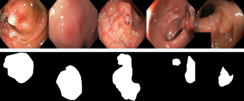
Figure 1: A few samples of the HyperKvasir dataset.

A few samples of the dataset are shown in Figure 1. The polyp images are RGB images, whereas the masks are single-channeled images. The mask colours the region with polyp white, while the surrounding regions are coloured black. This dataset was used to train our generative diffusion models, and compare the performance of the segmentation models depending on the type of training data used.

2.2 Pipeline Overview

The pipeline which we created generates data consisting of both images and masks. Our method foundationally relied on a generative diffusion model, the mechanism of which we present in Appendix A.1. Originally, we aim to train a diffusion model on the entire dataset, followed by styling of the images. However, we realized the need to narrow the scope of sampling and training to overcome the large variation between images. Thambawita et al [24] resolved this issue by training a dedicated GAN model for each image of the dataset. We improved this approach by adding more variation to the generated outputs. We do so by a procedure consisting of several steps illustrated in Figure 2

1. Cluster the images and masks in the dataset into groupss by similarity.

2. Train a diffusion model on each cluster, using a 4th channel input to generate the mask.

3. Use the image inpainting technique in [15] to modify the polyps in the images.

4. Style the resulting images using the methods of [12, 31].

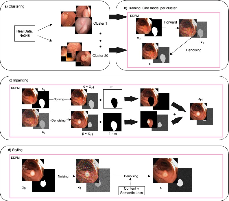
Figure 2: Schematic of our method. Given a dataset of real images and masks (here $N=348$), we a) cluster the images and masks by similarity into 20 clusters, b) train a diffusion model on each cluster, c) use the trained diffusion model and the inpainting technique to generate synthetic images and masks, and d) style the synthetic images by guiding the reverse diffusion process with various losses. DDPM = Denoising Diffusion Probabilistic Model.

2.3 Image Preprocessing

We first used the PyTorch Inception-v3 model pretrained on ImageNet to obtain a feature set for all images (including the masks) in the dataset. Next, we used scikit-learn’s KMeans algorithm to obtain 20 clusters of images. See Figure 3 for examples of images in such clusters; each row depicts images in one cluster. The images and masks were then resized to $256\times 256$ and pixel values scaled to $[-1,1]$.

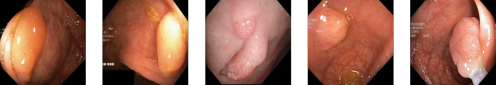
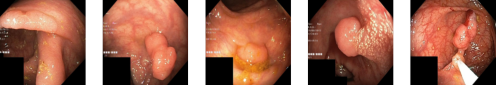
Figure 3: Example of clustering results. Each row consists of images from a cluster.

2.4 Training

We trained our diffusion model one by one for each cluster we created. Although clustering adds to the number of models trained and hence requires more compute, in our use case of small datasets, the number of clusters needed to sensibly group similar images is small. Hence, the extra compute and time is mild in practice.

In order to train the model to generate labels, we concatenated the mask as a 4th input channel. Our method inherited from the diffusion model implementation of [12] and the generation technique of [24].

The model was trained for 110,000 iterations with hyperparameters given in Appendix B.3. Moreover, we trained one additional model on the entire dataset to ablate the effectiveness of clustering. This model was trained on the same parameters for 200,000 iterations. The models were trained on Mist, a SciNet GPU cluster [14, 20]; each node of the cluster has 4 NVIDIA V100-SMX2-32GB GPU. The training time for each model was at most 16 hours, with variation resulting from cluster size.

2.5 Image Generation

After training the generative diffusion models, we generated 3 random samples for each real image using the inpainting technique introduced in [15] (Appendix A.1.1) with the parameters given in Appendix B.3. This procedure used the polyp mask to obscure the region of the image coloured white in the mask. The diffusion model is thus tasked with filling in this gap. The upside of this procedure as compared to generating the full image is that we conditioned the diffusion model on the surrounding region. This significantly contributed to the realism of the image, while also injecting sufficient variation to the image.

Note that a number of the polyp masks failed to obscure the entire polyp, and thus, the model recognized the polyp in its training set and returned the original image. To mitigate this, we dilated the polyp mask by 20 pixels which reduced the number of such cases.

Finally, we used a combination of the styling methods in [12, 31] to generate the final synthetic images. In particular, after sampling $348\times 3$ inpainted images, the style transfer procedure [12, 31] was applied to each image. A NVIDIA RTX A6000 was used for this procedure, which was carried out by the previously trained diffusion model. Each image required about 1 minute to style. The hyperparameters of this procedure are given in Appendix B.3.

We combined the two methods by applying [31] for the content loss and [12] for the style loss. This takes advantage of the improvements in [31] while using a style loss that does not require a text prompt. The total loss is the sum of the content and style loss; refer to Appendix A.1.2 for loss details.

2.6 Intrinsic Evaluation

To evaluate our samples, we did a qualitative expert review, and computed the Fréchet Inception Distance (FID) [7] and Multi-Scale Structural Similarity (MS-SSIM) [28] between the output images and the real data.

The FID [7] and MS-SSIM [28] scores measures the distance between the output images and the dataset, as well as the variance of the output images. Parmar et al [18] showed that differences in image compression and resizing, among other factors may induce significant variation in the FID scores. Hence, we used the method introduced in [18] to compute the FID.

For later convenience, we introduce the following convention when referring to each data type:

• Real: Real images from the training set.

• GAN: Synthetic images generated by SinGAN-Seg [24], downloaded at https://osf.io/xrgz8/.

• Diff: Images generated using the inpainting technique by a diffusion model trained on a single cluster. No styling applied.

• Styled-Diff: Images generated using the inpainting technique by a diffusion model trained on a single cluster. Style transfer applied.

• Full-Diff: Images generated using the inpainting technique by a diffusion model trained on the full dataset. No styling applied.

• Full-Styled-Diff: Images generated using the inpainting technique by a diffusion model trained on the full dataset. Style transfer applied.

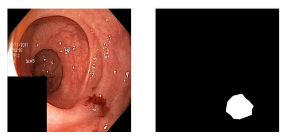
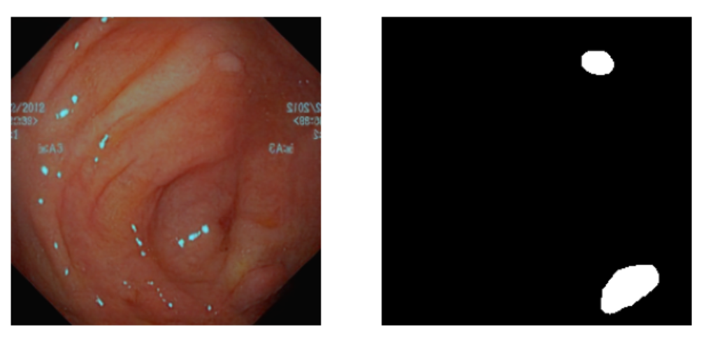
Figure 4: Example of survey images. Left pair is Real, whereas right pair is Fake.

For our expert review of the generated image, we had a radiologist (with 5 years of experience) review 30 shuffled images and their masks side by side; see Figure 4 for a sample. Out of these 30 images, 10 were real images, 10 were from Diff, and 10 were from Styled-Diff. See Appendix B.1 for further details and results.

2.7 Experiments with segmentation models

Subsequently, we trained a polyp segmentation model [23] with the original and synthetic dataset to compare their mean IoU and DL with the target masks in order to evaluate their effect on model performance.

IoU $$=\frac{TP}{TP+FP+FN}$$ (1)

Dice Loss $$=1-\frac{2TP}{2TP+FP+FN}.$$ (2)

Specifically, we compared the performance of the model when trained under standard augmentation methods, namely, with cropping and rotation, with synthetic data generated by [24], and with our synthetic data. We ran two sets of experiments:

• Full Synthetic Training: The model was trained on the entire synthetic dataset.

• Augmented Synthetic Training of Small Datasets: The model was trained on a dataset consisting of a subset ($N=16,32,64,128$) of real images augmented with synthetic images.

Full Synthetic Training.

We used the model proposed by Thambawita et al [23]; see Appendix B.2 for details. We performed three runs, each labeled "Type-N", where $N=1,2,3$ and Type represents which of the synthetic sets were used. The experiment Diff-N, for example, means that $N\times 348$ images were used in the training set, all chosen from the diffusion model output without styling. These were split into training (80%) and validation (20%) sets. For the test set, we used the HyperKvasir [1] dataset at https://datasets.simula.no/hyper-kvasir/, which contains 1000 images with corresponding masks. We selected images not used in the 348-size training set, and randomly chose 200 of these images as the test set. Tests were conducted on the best checkpoint, as determined by the validation IoU score.

Augmentation of Small Datasets.

We also experimented with the effect of augmentation on model performance when data is scarce. We followed the approach of Trabucco et al [26] when performing augmentation. In particular, we fix $\alpha\in(0,1)$, and sample indices $i,j$ uniformly

$$i\sim U({1,\ldots,N}),\quad j\sim U({1,\ldots,M})$$

where $N$ is the number of images in the training set and $M$ is the number of synthetic images per real image – in our case $N\in\{16,32,64,128\},M=3$. In Trabucco et al [26], $\alpha=0.5$ was set as the probability a synthetic image $\tilde{X}_{ij}$ generated from real image $X_{i}$ would be added to the training set. However, as it is typically the case that we have more synthetic data per real image, instead of simple addition with probabilty $\alpha=0.5$, we add $r=1,2,$ or $3$ synthetic images generated from $X_{i}$. Because of resource and time limitations, we restrict our attention to Styled-Diff and GAN. The experiments used the same parameters as those in the Full Synthetic Training experiments.

2.8 Statistical Analysis

Mean and standard deviation of FID and MS-SSIM were reported along with dependent t-test p-values. In full synthetic training, the DL and IoU mean and standard deviation were reported across $N=1,2,3$; significance computed using dependent t-test. Same was done in the small dataset experiments across $r=1,2,3$ for each $N=16,32,64,128$. A significance level of $P<0.05$ was used. All analyses were conducted using Python 3.10.9 with numpy 1.24.4 and scipy 1.11.1 as appropriate.

3 Results

3.1 Image Generation

The real data points were used as input to the diffusion models, and the segmentation mask is used as the inpainting mask. Recall that we are using a four-channel model, the last used by the segmentation mask. Consequently, our inpainting procedure generated a new image and its corresponding segmentation, alleviating much work for image annotators. Four real training images and three corresponding inpainted images are depicted in Figure 5. The first column of each subfigure represents the original image; the mask of each image is directly beneath it.

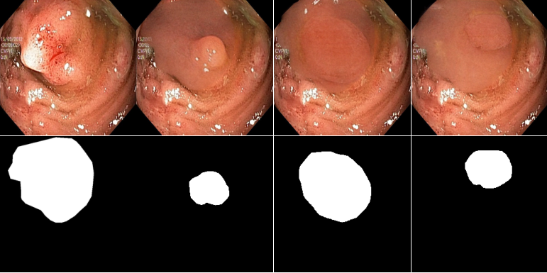
(a)

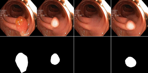
(b)

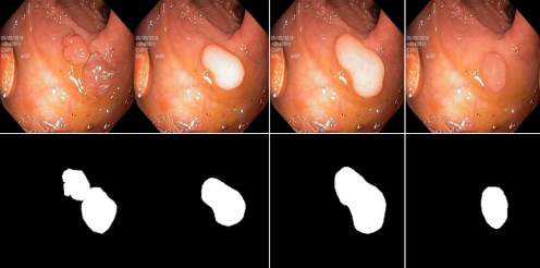
(c)

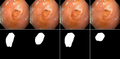
(d)

Figure 5: Example of inpainting results. Each subpart corresponds to a different source image; the first column is the source image, and the subsequent columns are synthetically generated using image inpainting. The corresponding segmentation mask is generated simultaneously with the image.

The styling results are depicted in Figure 6. The first row of each subfigure corresponds to the first row of each subfigure in Figure 5, whereas the second row is the styled image. By visual comparison in Figure 6, we see that styling improved the appearance of the synthetic images. This was done by smoothing out the inpainting region so as to remove the sudden changes in colour at the boundary of the inpainting region.

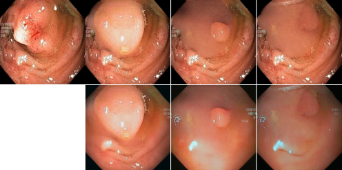
(a)

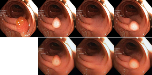
(b)

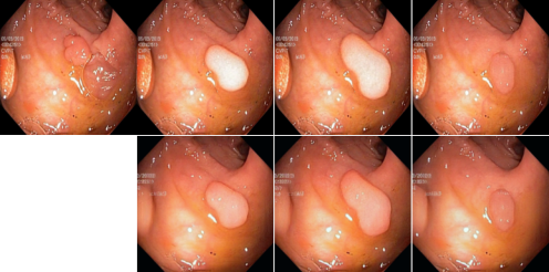
(c)

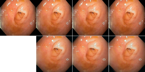
(d)

Figure 6: Example of styled results. Each subpart corresponds to a different source image; the first column is the source image, and the subsequent columns compare the image with (second row) and without styling (first row). The corresponding segmentation mask remains the same after this process.

3.2 Intrinsic evaluation

The FID and MS-SSIM values are reported in Table 1. The FID of Styled-Diff ($65.99\pm 0.37$) is significantly different from the other datasets ($P<0.002$). In particular, this means it is significantly closer to the real images than GAN, but significantly farther than the other variations on Diff. Moreover, the variations on Diff obtained a significantly lower FID than GAN, indicating that they are more alike the real image. It is also true for MS-SSIM that Styled-Diff ($0.2346\pm 0.0062$) is significantly greater than the other datasets, including Real, ($P<0.05$). Moreover, the MS-SSIM values of the synthetic data fall within $0.05$ of the Real data, indicating that the variance of the synthetic data is similar to the real data. This is expected as the diffusion model is trained on the real dataset, and the inpainting technique may only add elements from other images in the dataset.

Table 1: Fréchet Inception Distance (FID) and Multi-Scale Structural Similarity (MS-SSIM) comparison between real and synthetic images. Images are shuffled, and each data type (including Real) is compared with Real. The computations were performed thrice.

Data type			FID			MS-SSIM
			Set 1	Set 2	Set 3	Set 1	Set 2	Set 3
Real				$-4.412\cdot 10^{-5}$			0.1813
GAN			118.73	119.45	116.92	0.1986	0.2004	0.2037
Diff			36.01	37.90	37.78	0.2081	0.2126	0.2096
Styled-Diff			66.17	65.48	66.32	0.2304	0.2300	0.2433
Full-Diff			40.59	40.77	40.27	0.2030	0.2058	0.2078
Full-Styled-Diff			60.15	59.98	59.95	0.1971	0.1924	0.1969

We should be careful in interpreting the FID metric because our inpainting technique necessarily leaves parts of the original image intact. Our caution is supported by the fact that our pipeline without styling has a lower FID than the styled pipeline. For instance, in Figure 6(a), the styled image shows a drastic change in the surroundings so as to better match the inpainted region. On one hand, this smoothening effect created a more natural appearance, but on the other, it increased the distance between the synthetic and real images. However, as we see in Figure 6, the images without styling contains noticeable sudden changes in colour at the inpainting region, resulting in an unnatural appearance. Thus, despite the visual improvement FID is higher after styling. Furthermore, for our purpose of training segmentation models, some deviation from the real images is desirable as we want to avoid overfitting to the real images.

3.3 Experiments with segmentation models

Full Synthetic Training.

In addition to the intrinsic evaluations above, we evaluated the synthetic images by training a segmentation model. The results are given in Table 2.

Table 2: Performance evaluation of the segmentation model entirely trained on synthetic data. Values reported are Dice Loss and Intersection over Union (IoU) scores.

Data type			Scores
			Dice Loss	IoU
Real			0.1320	0.8085
GAN-1			0.3447	0.5790
Diff-1			0.3434	0.5948
Styled-Diff-1			0.2556	0.6840
Full-Diff-1			0.3189	0.6149
Full-Styled-Diff-1			0.3486	0.5751
GAN-2			0.2938	0.6239
Diff-2			0.3374	0.5975
Styled-Diff-2			0.2272	0.7027
Full-Diff-2:			0.3403	0.5983
Full-Styled-Diff-2			0.3923	0.5534
GAN-3			0.3040	0.6256
Diff-3			0.3484	0.5883
Styled-Diff-3			0.1958	0.7396
Full-Diff-3			0.3915	0.5501
Full-Styled-Diff-3			0.4351	0.5213

In our first segmentation experiment, shown in Table 2, we trained the model only using generated data and tested using real data not used in the generation. We see that Styled-Diff, averaging across $N=1,2,3$, had a DL and IoU of $0.2262\pm 0.02442$ and $0.7088\pm 0.0231$ respectively, trailing behind the real data by about $0.12$ in both metrics. This performed better than GAN data which achieved $0.3142\pm 0.0220;0.6095\pm 0.0216$ with both $P<0.02$. Moreover, styling resulted in significant improvement in the Dice loss and IoU scores: Diff achieved $0.3431\pm 0.0045;0.5935\pm 0.0039;$, significantly lower than Styled-Diff $P<0.03$. The effect of clustering can also be observed: Full-Styled-Diff achieved $0.3920\pm 0.0353;0.5450\pm 0.0221$, but this difference is only significant in IoU ($P_{DL}=0.0592;P_{IoU}=0.0381$).

Augmentation of Small Datasets.

The results are given in Table 3. In contrast to augmenting full datasets, when augmenting small datasets, the synthetic data performed better than Real with standard augmentation techniques (Appendix B.2). This is because the synthetic data incorporated elements from images not in the training set, and thus contributed new information. Indeed, this effect is most noticeable when the training set is starved for data, such as when $N=16$, where the largest improvement in the DL and IoU scores (Styled-Diff: $0.5065\pm 0.0288;0.5990\pm 0.0060$ and GAN: $0.5137\pm 0.0100;0.5761\pm 0.0084$ with $P<0.04$ for both metrics) occurs. Moreover, the effect diminishes as the training set size increases. However, the improvement in both metrics is still significant for $16<N<128$ ($P<0.05$) – with the exception of $P_{IoU}=0.104$ for Real vs GAN when $N=32$. It is also worth noting when the difference between Styled-Diff and GAN are significant; this occurs when $N=16$ where $P_{IoU}=0.0087$.

Table 3: Performance evaluation of the segmentation model when small training sets are augmented by synthetic images. Augmentation strategy: with probability 0.5, replace each real image with $r$ synthetic images. Values reported are Dice Loss and Intersection over Union (IoU) scores.

$N$	Data type			Scores, $r=1$		Scores, $r=2$		Scores, $r=3$
				Dice Loss	IoU	Dice Loss	IoU	Dice Loss	IoU
16	Real					0.6056	0.5263
	Styled-Diff			0.4838	0.5930	0.4886	0.5968	0.5471	0.6072
	GAN			0.5165	0.5658	0.5003	0.5762	0.5243	0.5863
32	Real					0.5580	0.6201
	Styled-Diff			0.4366	0.6494	0.3392	0.6690	0.2856	0.6812
	GAN			0.4136	0.6326	0.3413	0.6609	0.2695	0.6765
64	Real					0.4201	0.6930
	Styled-Diff			0.2845	0.7262	0.2851	0.7133	0.2187	0.7294
	GAN			0.2420	0.7184	0.2976	0.7142	0.2493	0.7098
128	Real					0.1768	0.7982
	Styled-Diff			0.1878	0.7511	0.2281	0.7525	0.2227	0.7494
	GAN			0.1770	0.7536	0.1900	0.7513	0.1927	0.7511

4 Discussion

In this paper, we explored the use of diffusion models and related techniques to generate synthetic data for medical image segmentation. We evaluated the output images as a result of inpainting and styling. Furthermore, we evaluated automatic segmentation models when fully or partially trained with our synthetic images. We found that diffusion models are a viable method of generating realistic synthetic data, and that styling improves the appearance of the synthetic images. Moreover, we found that when a segmentation model is trained using synthetic data from our diffusion pipeline, the model performs better than when trained using SinGAN-Seg generated data [24]. This improvement can also be seen in the case of augmenting small datasets.

Our results therefore suggest that data generated by our pipeline may be used to either: replace real data in the training set, or augment real data in small training sets. In the former case, we saw that the synthetic data performs better than the SinGAN-Seg generated data [24], and in the latter case, we saw an improvement over the Real data and GANs for $N<128$. As opposed to manual gathering and labeling of data, our pipeline is fully automated and thus can be used to generate large amounts of data with minimal human effort. In particular, our pipeline may increase the size and quality of small datasets by generating an arbitrary number of synthetic images from one real image.

In contrast to work by Pishva et al [19], Du et al [4], our work used a fourth channel to generate the segmentation mask. This allowed us to generate the segmentation mask simultaneously with the image, and thus, alleviate the need for extra models to generate the mask. Moreover, we explored the RePaint technique when the polyps were the subject being inpainted onto the source image, as opposed to the method by Pishva et al [19] which inpainted the background. This generally resulted in a more realistic image. We also used a combination of styling techniques to improve the appearance of the synthetic images which was not explored in either work.

Our study has several limitations. First, we only used one dataset in our paper. The application of our technique to other, small, low-similarity image segmentation datasets may be done to reinforce the results in this paper. Second, the metrics we used to evaluate the synthetic images are not perfect, especially in the realm of medical images. Therefore, caution has to be exercised when interpreting the results. Finally, in this paper, we were constrained by time and computational resources to only explore 3 image samples per real image. It was shown by Fort et al [5] that multiple augmentations per image can improve performance. Thus, it would be interesting to explore the effect of increasing the number of synthetic images per real image and augmenting with $N>3$ images. Other than the recommendations above, another avenue for future work is the effect of using differentially-private diffusion models [6]. If such models do not compromise performance, then we may extend our method to a wider range of datasets and enable the use of our pipeline as an image-sharing technique, i.e. instead of original images, we may instead share images generated from them.

In summary, our pipeline can be used to generate more realistic synthetic data for medical image segmentation. This data can be used to augment small datasets, or replace the real data in the training set. In particular, we see that our pipeline outperforms SinGAN-generated data [24] in both cases, and styling sufficiently improves the appearance of the synthetic images to be used in training.

Statements and Declarations

Authors’ Contributions

Conceptualization: D.S., P.N.T.; Methodology: D.S.; Formal analysis and investigation: D.S.; Writing - original draft preparation: D.S.; Writing - review and editing: D.S., P.N.T.; Supervision: P.N.T.

Funding

The authors did not receive support from any organization for the submitted work.

Data Availability

The data used in this study is publicly available at https://datasets.simula.no/hyper-kvasir/ (HyperKvasir) and https://osf.io/xrgz8/ (SinGAN-Seg). The generated samples are also available at https://osf.io/ts6px/.

Code Availability

The custom code used in this paper is available on GitHub at https://github.com/dsaragih/diffuse-gen.

Competing Interests

D.S. has no competing interests to declare. P.N.T. has received research support from Nippon Steel and Novo Nordisk. P.N.T. has received a speaker honorarium from Novo Nordisk and receives consulting fees from Novo Nordisk.

Ethics approval

Not applicable.

Consent to participate

Not applicable.

Consent for publication

Not applicable.

Appendix A Background

A.1 Background on Diffusion Models

Diffusion models were first formulated by Ho et al [8] and later improved by Nichol and Dhariwal [17]. The diffusion model consists of two primary components: the forward diffusion process, denoted $q$, and the reverse denoising process, denoted $p$. Starting at a clean image $x_{0}$, we gradually add Gaussian noise to it for $T$ timesteps. In particular,

$$q(x_{T}|x_{0})=\prod_{t=1}^{T}q(x_{t}|x_{t-1})$$

where

$$q(x_{t}|x_{t-1})=\mathcal{N}(x_{t};\sqrt{1-\beta_{t}}x_{t-1},\beta_{t}(1-\beta_{t})I),$$

and where $\beta_{1},\ldots,\beta_{T}$ is the variance schedule (e.g. the one proposed by Nichol and Dhariwal [17]), and $x_{T}$ is the noisy image. We can however reparameterize the distribution by letting $\alpha_{t}:=1-\beta_{t}$ and $\bar{\alpha}_{t}:=\prod_{r=1}^{t}\alpha_{r}$. Then, we may sample any $t\in\{1,\ldots,T\}$ directly by

$$x_{t}=\sqrt{\bar{\alpha}_{t}}x_{0}+\sqrt{1-\bar{\alpha}_{t}}\epsilon_{t},\quad\epsilon_{t}\sim\mathcal{N}(0,I).$$ (3)

The reverse denoising process is the process of denoising the noisy image $x_{T}$ to recover the clean image $x_{0}$. This process may only be approximated, and is the component of the model which is learned. In particular, we learn to maximize the variational lower bound by gradual transitions $p_{\theta}(x_{t-1}|x_{t})$ determined by the model parameters $\theta$. Starting at $p(x_{T})=\mathcal{N}(x_{T};0,I)$, we obtain

$$p_{\theta}(x_{0:T})=p(x_{T})\prod_{t=1}^{T}p_{\theta}(x_{t-1}|x_{t}),$$

where

$$p_{\theta}(x_{t-1}|x_{t})=\mathcal{N}(x_{t-1};\mu_{\theta}(x_{t},t),\Sigma_{\theta}(x_{t},t)).$$

The parameters above are what we would like to learn. Nichol and Dhariwal [17] described a method to learn $\Sigma_{\theta}(x_{t},t)$, which we employ in our training. However, most important is

$$\mu_{\theta}(x_{t},t):=\frac{1}{\sqrt{\bar{\alpha}_{t}}}\left(x_{t}-\frac{1-\alpha_{t}}{\sqrt{1-\bar{\alpha}_{t}}}\epsilon_{\theta}(x_{t},t)\right).$$

Ho et al [8] found that it was best to optimize the "noise" term, $\epsilon_{\theta}(x_{t},t)$. In particular, the objective is

$$\min_{\theta}\mathbb{E}_{t,x_{0},\epsilon}\left[\|\epsilon-\epsilon_{\theta}(x_{t},t)\|^{2}\right].$$

We may then predict $x_{t-1}$ by

$$x_{t-1}=\mu_{\theta}(x_{t},t)+\sigma_{t}\epsilon,$$ (4)

and henceforth obtain the final prediction $\hat{x}_{0}$.

A.1.1 Using Diffusion Models for Image Inpainting

The technique of inpainting with diffusion models were first introduced by Lugmayr et al [15]. The approach involves a mask $m$ with pixel values either 0 or 1, where 0 indicates the unknown regions, i.e. regions we would like to paint in, and 1 indicates known regions, i.e. regions we would like to maintain. A simple modification of the reverse denoising process is needed to achieve this goal. Suppose we wish to obtain $x_{t-1}$ from $x_{t}$. We only want the denoising process to take place on the unknown region of the mask, hence we use Equation 3 to obtain the known regions: $x_{t-1}^{known}=m\odot x_{t-1}$, and then use Equation 4 to obtain the unknown regions: $x_{t-1}^{unknown}=(1-m)\odot x_{t-1}$. We then combine the two:

$$x_{t-1}=x_{t-1}^{known}+x_{t-1}^{unknown}.$$ (5)

A.1.2 Using Diffusion Models for Image Styling

In our pipeline, the technique of using diffusion models for styling is based on the work of Kwon and Ye [12], Yang et al [31]. The method works by having a designated target image, which we use to guide the translation of the source image. In our case, the source image will be the image generated via inpainting by our diffusion model, and the target image is the original image which was inpainted. The objective of image translation is to preserve the structural content, while varying the semantic content to better match the target. As such, we have two general sets of losses: content and style loss. These conditional losses are applied at each reverse timestep $t$. In particular, if we let $\ell_{total}$ be the style loss, then like in Equation 4, we obtain

$$x_{t-1}^{\prime} =\mu_{\theta}(x_{t},t)+\sigma_{t}\epsilon,\quad\epsilon\sim\mathcal{N}(0,I)$$

$$x_{t-1} =x_{t-1}^{\prime}-\nabla_{x_{t}}\ell_{total}({\hat{x}}_{0}(x_{t})),$$

where $\hat{x}_{0}(x_{t})$ is the predicted clean image from the noisy sample at timestep $t$ obtained using Tweedie’s formula [11]. For our convenience, we write $x:=\hat{x}_{0}(x_{t})$.

We first focus our attention to the content losses. In this case, we make use of the losses in [31]: $\ell_{ZeCon},\ell_{VGG}$ The ZeCon loss takes in $x,x_{0}$ – note that $x_{0}$ is the target image – and forwards them to the UNet, i.e. the estimator of $\epsilon_{\theta}(x_{t},t)$. The UNet encoder is used to extract feature maps at some layer $l$ of both $x$ and $x_{t}$; we denote their respective feature maps $\hat{z}_{l}$ and $z_{l}$. We then randomly select a spatial location on the feature $z_{l}$ from the set of all locations $s\in\{1,\ldots,S_{l}\}=:S$ on which we compute the cross-entropy loss. The Zecon loss is then

$$\ell_{ZeCon}(x,x_{0}):=\mathbb{E}_{x_{0}}\left[\sum_{l}\sum_{s}\mathcal{L}_{CE}(\hat{z}_{l}^{s},z_{l}^{s},z_{l}^{S\setminus s})\right]$$ (6)

The VGG loss is defined simply as the MSE between VGG feature maps of $x,x_{0}$.

Next, we deal with the style losses which we take adapt from [12]: $\ell_{sty},\ell_{L2},\ell_{sem},\ell_{rng}$. A primary component of our losses is the DINO ViT [3] which was shown by Tumanyan et al [27] to delineate between structural content and semantic content. In particular, the [CLS] token of the last layer was shown to contain semantic information; we will follow Kwon and Ye [12] and denote it $e^{L}_{[CLS]}(\cdot)$.

The primary semantic style loss we use is $\ell_{sty}$:

$$\ell_{sty}(x,x_{0}):=\|e^{L}_{[CLS]}(x_{0})-e^{L}_{[CLS]}(x)\|_{2}.$$ (7)

In order to accelerate the generation process, we wish to maximize the semantic distance between the estimated clean images of adjacent timesteps. Therefore, we define $\ell_{sem}$ as follows:

$$\ell_{sem}(x_{t},x_{t-1}):=-\|e^{L}_{[CLS]}(\hat{x}_{0}(x_{t-1}))-e^{L}_{[CLS]}(\hat{x}_{0}(x_{t}))\|_{2}.$$ (8)

The losses $\ell_{L2},\ell_{rng}$ are defined more simply: the former is just the MSE of the pixel difference between $x,x_{0}$, and the latter is a regularization loss to prevent irregular steps in the reverse process. We thus have:

$$\mathcal{L}_{content} =\lambda_{ZeCon}\ell_{ZeCon}(x,x_{0})+\lambda_{VGG}\ell_{VGG}(x,x_{0})$$

$$\mathcal{L}_{style} =\lambda_{sty}\ell_{sty}(x,x_{src})+\lambda_{L2}\ell_{L2}(x,x_{src})+\lambda_{sem}\ell_{sem}(x_{t};x_{t-1})+\lambda_{rng}\ell_{rng}$$

$$\mathcal{L}_{total} =\mathcal{L}_{content}+\mathcal{L}_{style}$$

where $x_{0}$ is the inpainted image and $x_{src}$ is the real image which was inpainted.

Appendix B Further Methods and Results

B.1 Expert Review

Three assessments were made: image quality, segmentation quality, and whether the image was real or synthetic. The image and segmentation quality assessments had 3 options: Good, Moderate, and Poor. Using this data, accuracy, recall, and precision were calculated to measure the agreement in the classification of real vs. fake images.

The results of the expert review are shown in Table 4. Combining the Diff and Styled-Diff sets as the "Fake" set of images, we obtain an accuracy, precision, and recall of 60%, 40%, and 40% respectively.Moreover, this review confirms that the generations are indeed good quality data points, although some may identified as synthetic. It is also interesting to see how the real images were rated since it was the category with the highest number of fake images identified.

Table 4: Survey results from an expert rater tasked with assessing image quality, segmentation quality, and whether the image was real or synthetic.

			Image Quality			Segmentation Quality			Real or Fake
Data type			Good	Moderate	Poor	Good	Moderate	Poor	Real	Fake
Real			10	0	0	8	2	0	4	6
Diff			10	0	0	10	0	0	3	7
Styled-Diff			10	0	0	9	1	0	3	7

B.2 Segmentation Model Training Details

The model used in [23] employs a UNet++ backbone. Specifically, the model was trained only using the generated data and tested using real data. We used the se_resnext50_32x4d network as the UNet++ encoder and softmax2d as the last layer activation function. PyTorch was used as the devlopment framework, and the data stream was handled by PYRA along with the Albumentations augmentation library. The standard training augmentations used were: ShiftScaleRotate, HorizontalFlip, and one of CLAHE, RandomBrightness, RandomGamma. The model weights were zero-initialized and they were trained for 150 epochs, with a learning rate of 0.0001 for the first 50 epochs, which was reduced to 0.00001 for the remaining epochs.

B.3 Hyperparameters

For our implementation of the diffusion model, our sampling number is set to be $T=200$, but we skipped the first 80 timesteps. The images were resized to be $256\times 256$ and the diffusion model had 4 input channels (+1 to accomodate the mask). Moreover, when inpainting the image, we set the jump length $j=10$ with $r=5$ times resampling; these parameters are described further in Lugmayr et al [15]. For styling, we used $\lambda_{ZeCon}=500,\lambda_{VGG}=100,\lambda_{MSE}=5000,\lambda_{sty}=10000,\lambda_{L2}=10000,\lambda_{sem}=40000,\lambda_{rng}=200$. For the ViT model used to compute the style and semantic losses, we used the DINO-ViT model [27] which used the same settings as in Kwon and Ye [12].

References

- \bibcommenthead
- Borgli et al [2020] Borgli H, Thambawita V, Smedsrud PH, et al (2020) HyperKvasir, a comprehensive multi-class image and video dataset for gastrointestinal endoscopy. Scientific Data 7(1):283. 10.1038/s41597-020-00622-y
- Borji [2023] Borji A (2023) Generated Faces in the Wild: Quantitative Comparison of Stable Diffusion, Midjourney and DALL-E 2. 10.48550/arXiv.2210.00586, 2210.00586
- Caron et al [2021] Caron M, Touvron H, Misra I, et al (2021) Emerging Properties in Self-Supervised Vision Transformers. In: Proceedings of the IEEE/CVF International Conference on Computer Vision, pp 9650–9660
- Du et al [2023] Du Y, Jiang Y, Tan S, et al (2023) ArSDM: Colonoscopy Images Synthesis with Adaptive Refinement Semantic Diffusion Models. In: Greenspan H, Madabhushi A, Mousavi P, et al (eds) Medical Image Computing and Computer Assisted Intervention – MICCAI 2023. Springer Nature Switzerland, Cham, Lecture Notes in Computer Science, pp 339–349, 10.1007/978-3-031-43895-0_32
- Fort et al [2022] Fort S, Brock A, Pascanu R, et al (2022) Drawing Multiple Augmentation Samples Per Image During Training Efficiently Decreases Test Error. 10.48550/arXiv.2105.13343, 2105.13343
- Ghalebikesabi et al [2023] Ghalebikesabi S, Berrada L, Gowal S, et al (2023) Differentially Private Diffusion Models Generate Useful Synthetic Images. 10.48550/arXiv.2302.13861, 2302.13861
- Heusel et al [2017] Heusel M, Ramsauer H, Unterthiner T, et al (2017) GANs Trained by a Two Time-Scale Update Rule Converge to a Local Nash Equilibrium. In: Advances in Neural Information Processing Systems, vol 30. Curran Associates, Inc.
- Ho et al [2020] Ho J, Jain A, Abbeel P (2020) Denoising Diffusion Probabilistic Models. In: Advances in Neural Information Processing Systems, vol 33. Curran Associates, Inc., pp 6840–6851
- Jiang et al [2017] Jiang F, Jiang Y, Zhi H, et al (2017) Artificial intelligence in healthcare: Past, present and future. Stroke and Vascular Neurology 2(4). 10.1136/svn-2017-000101
- Khader et al [2023] Khader F, Müller-Franzes G, Tayebi Arasteh S, et al (2023) Denoising diffusion probabilistic models for 3D medical image generation. Scientific Reports 13(1):7303. 10.1038/s41598-023-34341-2
- Kim and Ye [2021] Kim K, Ye JC (2021) Noise2Score: Tweedie’s Approach to Self-Supervised Image Denoising without Clean Images. In: Advances in Neural Information Processing Systems, vol 34. Curran Associates, Inc., pp 864–874
- Kwon and Ye [2023] Kwon G, Ye JC (2023) Diffusion-based Image Translation using Disentangled Style and Content Representation. 10.48550/arXiv.2209.15264, 2209.15264
- Lindner et al [2019] Lindner L, Narnhofer D, Weber M, et al (2019) Using Synthetic Training Data for Deep Learning-Based GBM Segmentation. In: 2019 41st Annual International Conference of the IEEE Engineering in Medicine and Biology Society (EMBC), pp 6724–6729, 10.1109/EMBC.2019.8856297
- Loken et al [2010] Loken C, Gruner D, Groer L, et al (2010) SciNet: Lessons Learned from Building a Power-efficient Top-20 System and Data Centre. Journal of Physics: Conference Series 256(1):012026. 10.1088/1742-6596/256/1/012026
- Lugmayr et al [2022] Lugmayr A, Danelljan M, Romero A, et al (2022) RePaint: Inpainting using Denoising Diffusion Probabilistic Models. In: 2022 IEEE/CVF Conference on Computer Vision and Pattern Recognition (CVPR), pp 11451–11461, 10.1109/CVPR52688.2022.01117
- Navarro et al [2019] Navarro F, Shit S, Ezhov I, et al (2019) Shape-Aware Complementary-Task Learning for Multi-organ Segmentation. In: Suk HI, Liu M, Yan P, et al (eds) Machine Learning in Medical Imaging. Springer International Publishing, Cham, Lecture Notes in Computer Science, pp 620–627, 10.1007/978-3-030-32692-0_71
- Nichol and Dhariwal [2021] Nichol AQ, Dhariwal P (2021) Improved Denoising Diffusion Probabilistic Models. In: Proceedings of the 38th International Conference on Machine Learning. PMLR, pp 8162–8171
- Parmar et al [2022] Parmar G, Zhang R, Zhu JY (2022) On Aliased Resizing and Surprising Subtleties in GAN Evaluation. In: Proceedings of the IEEE/CVF Conference on Computer Vision and Pattern Recognition, pp 11410–11420
- Pishva et al [2023] Pishva AK, Thambawita V, Torresen J, et al (2023) RePolyp: A Framework for Generating Realistic Colon Polyps with Corresponding Segmentation Masks using Diffusion Models. In: 2023 IEEE 36th International Symposium on Computer-Based Medical Systems (CBMS), pp 47–52, 10.1109/CBMS58004.2023.00190
- Ponce et al [2019] Ponce M, van Zon R, Northrup S, et al (2019) Deploying a Top-100 Supercomputer for Large Parallel Workloads: The Niagara Supercomputer. In: Proceedings of the Practice and Experience in Advanced Research Computing on Rise of the Machines (Learning). Association for Computing Machinery, New York, NY, USA, PEARC ’19, pp 1–8, 10.1145/3332186.3332195
- Pratondo et al [2017] Pratondo A, Chui CK, Ong SH (2017) Integrating machine learning with region-based active contour models in medical image segmentation. Journal of Visual Communication and Image Representation 43:1–9. 10.1016/j.jvcir.2016.11.019
- Shin et al [2018] Shin Y, Qadir HA, Balasingham I (2018) Abnormal Colon Polyp Image Synthesis Using Conditional Adversarial Networks for Improved Detection Performance. IEEE Access 6:56007–56017. 10.1109/ACCESS.2018.2872717
- Thambawita et al [2021] Thambawita V, Hicks SA, Halvorsen P, et al (2021) DivergentNets: Medical Image Segmentation by Network Ensemble. 10.48550/arXiv.2107.00283, 2107.00283
- Thambawita et al [2022] Thambawita V, Salehi P, Sheshkal SA, et al (2022) SinGAN-Seg: Synthetic training data generation for medical image segmentation. PLOS ONE 17(5):e0267976. 10.1371/journal.pone.0267976
- Trabucco et al [2023a] Trabucco B, Doherty K, Gurinas M, et al (2023a) Effective Data Augmentation With Diffusion Models. 2302.07944
- Trabucco et al [2023b] Trabucco B, Doherty K, Gurinas M, et al (2023b) Effective Data Augmentation With Diffusion Models. 2302.07944
- Tumanyan et al [2022] Tumanyan N, Bar-Tal O, Bagon S, et al (2022) Splicing ViT Features for Semantic Appearance Transfer. In: Proceedings of the IEEE/CVF Conference on Computer Vision and Pattern Recognition, pp 10748–10757
- Wang et al [2003] Wang Z, Simoncelli E, Bovik A (2003) Multiscale structural similarity for image quality assessment. In: The Thrity-Seventh Asilomar Conference on Signals, Systems & Computers, 2003, pp 1398–1402 Vol.2, 10.1109/ACSSC.2003.1292216
- Willemink et al [2020] Willemink MJ, Koszek WA, Hardell C, et al (2020) Preparing Medical Imaging Data for Machine Learning. Radiology 295(1):4–15. 10.1148/radiol.2020192224
- Xu et al [2019] Xu Y, Wang Y, Yuan J, et al (2019) Medical breast ultrasound image segmentation by machine learning. Ultrasonics 91:1–9. 10.1016/j.ultras.2018.07.006
- Yang et al [2023] Yang S, Hwang H, Ye JC (2023) Zero-Shot Contrastive Loss for Text-Guided Diffusion Image Style Transfer. 2303.08622
- Yu et al [2018] Yu KH, Beam AL, Kohane IS (2018) Artificial intelligence in healthcare. Nature Biomedical Engineering 2(10):719–731. 10.1038/s41551-018-0305-z