Learning Independent Program and Architecture Representations for Generalizable Performance Modeling

Abstract

This paper proposes PerfVec, a novel deep learning-based performance modeling framework that learns high-dimensional, independent/orthogonal program and microarchitecture representations. Once learned, a program representation can be used to predict its performance on any microarchitecture, and likewise, a microarchitecture representation can be applied in the performance prediction of any program. Additionally, PerfVec yields a foundation model that captures the performance essence of instructions, which can be directly used by developers in numerous performance modeling related tasks without incurring its training cost. The evaluation demonstrates that PerfVec is more general, efficient, and accurate than previous approaches.

1 Introduction

Performance modeling has been a practical area of emphasis and a computer science and engineering challenge since the beginning of the computing era. First, it is essential in performance characterization, verification, and optimization. It also provides a quantitative tool for architecture design space exploration, as well as codesign of architectures, applications, and system software to metrics of interest such as performance, power, or resilience. In addition, performance modeling is crucial to solve resource allocation problems. For example, cloud systems benefit from allocating the minimal resources to a job given an execution latency guarantee, and mobile operating systems may tune frequencies/voltages to minimize battery drain while satisfying performance goals.

Performance modeling approaches can be broadly categorized into three classes. The first involves simulating the program execution using discrete-event techniques and software simulators [12, 47]. Simulation is the default means in early hardware design stages due to its flexibility and ease of use, but its speed is plagued by high computational cost and limited parallelism. It is impractical to simulate real-world programs as a result. Second, performance can be evaluated using hardware emulators whose speed is close to native hardware [16, 31]. However, emulators are expensive to build and lack flexibility, because hardware implementation and verification require significant human expertise and efforts. The third general category is analytical modeling. Compared to simulators and emulators, analytical models are much faster because they use high-level abstractions, which are based on simplified assumptions of programs and microarchitectures. Analytical models try to capture various performance impact factors in abstract equations [58, 23, 52, 7, 27]. Due to the human-engineered nature of analytical models and the complexity of modern processors, they often ignore critical execution details and thus fall short in accuracy. Alternatively, recent work constructs analytical models using machine learning (ML) [28, 34, 4, 59, 36, 15, 22]. The most important drawback of existing ML-based analytical models is they are program and/or microarchitecture specific. This means that when target programs or microarchitectures change, new models must be trained, and consequently, new datasets must be acquired for training through simulation. Both data acquisition and model training are extremely time consuming and computationally expensive, severely limiting their practicality.

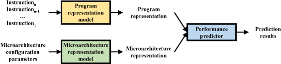
Figure 1: The proposed PerfVec framework based on independent and orthogonal program and microarchitecture representations.

In this work, we propose a performance modeling framework that is generalizable to any program and microarchitecture, PerfVec. PerfVec autonomously separates the performance impact of programs and microarchitectures by learning program and microarchitecture representations that are independent of and orthogonal to each other. In ML terminology, representations/embeddings are learned high-dimensional vectors that represent certain types of data (e.g., words [40], images [5], proteins [29]) for general understanding or specific tasks (e.g., language translation, image segmentation) [11]. Representation learning has been one of the core ideas behind ML’s great success. PerfVec employs separate models that aim to extract the key and essential performance characteristics from programs and microarchitectures, respectively.

PerfVec has four key advantages. First, PerfVec is the first program and microarchitecture independent/oblivious ML-based performance model, while existing ML-based modeling approaches need to create separate models for different programs or microarchitectures. In PerfVec, once a program’s representation is learned, it can be used to predict the performance of that program on any microarchitecture. Conversely, once a microarchitecture’s representation is learned, it can be used to predict the performance of any program running on that microarchitecture. Second, high-dimensional representations produced by PerfVec can capture subtle performance-relevant details unlike traditional human-engineered analytical models, thereby resulting in better prediction accuracy. Third, PerfVec has a fast prediction speed comparable with simple analytical models. Last but not least, training PerfVec yields a foundation model that captures the essential performance characteristics of instructions and has wide applicability. Users can use the pre-trained foundation model to learn the representation of any program compiled to the same instruction set architecture (ISA), without having to understand its training process or pay for its training overhead.

The contributions detailed in this paper are:

• We devise a novel performance modeling framework that autonomously learns to separate the performance impact of programs and microarchitectures. (Section 2)

• We create a foundation model to learn an instruction’s representation using neighbor instructions that it interacts with during execution. We rigorously prove that the representation of a program can be composed by the representations of all its executed instructions. The compositional property allows the foundation model to be generalizable to any program. (Section 3)

• To efficiently train the foundation model, we propose microarchitecture sampling and representation reuse. Together, they reduce the training time by several orders of magnitude. (Section 4)

• The evaluation shows that PerfVec can make accurate performance predictions for programs and microarchitectures that are not present during training, demonstrating its generality. We also visualize learned representations to demonstrate their meaningfulness. (Section 5)

• We demonstrate several applications of PerfVec, such as design space exploration and program analysis. PerfVec significantly accelerates design space exploration compared to existing approaches. (Section 6)

We plan to make the PerfVec framework and the pre-trained foundation model publicly available.

2 Toward Generalizable Performance Modeling

Performance is determined by the mapping of the running program onto the underlying microarchitecture and the interplay between their characteristics. As introduced in Section 1, a performance model captures this mapping either in a complete simulation/emulation run of all instructions using a detailed microarchitecture model, by a simplified mathematical model in human-engineered analytical modeling, or through a data-driven surrogate in ML-based analytical modeling, and each of these methodologies has its advantages and limitations. Simulation/emulation requires significant running time/human efforts, and human-engineered analytical models have low prediction accuracy as they fail to capture subtle execution details. While ML-based analytical models are much faster than simulation/emulation and also more accurate than human-engineered analytical models, they have poor generality as a trained model only works for certain programs and/or microarchitectures. Training a new model for different programs and microarchitectures is costly because acquiring new training data involves extensive and time-consuming simulation, and training itself is also computationally expensive.

This paper aims to solve the generality problem of existing ML-based models. A generalizable performance model should have a clear separation between the impact of programs and microarchitectures. Such “separation of concerns” minimizes the changes needed for the model when target programs or microarchitectures alter, and thus make it generalizable. To achieve this goal, we devise the PerfVec performance modeling framework that autonomously separates the performance impact of programs and microarchitectures. Figure 1 shows the overall architecture of PerfVec. It contains three ML models. First, a program representation model learns microarchitecture-independent program performance representations from program properties. The desirable representation of a program is fixed and can be used to predict its performance on any microarchitecture. Meanwhile, a counterpart microarchitecture representation model learns program-independent microarchitecture representations from microarchitecture configurations. Similarly, microarchitecture representations should be applicable to any program. Finally, a performance predictor makes predictions based on program and microarchitecture representations.

3 Compositional Representations

3.1 Challenges to Learn Program Representations

The biggest challenge of constructing PerfVec is building the program representation model. Previous ML models make use of high-level structural (e.g., data/control flow graphs [51]) and/or runtime (e.g., performance counters [59, 51]) information to learn representations for performance prediction. Because there does not exist a set of high-level information that includes all performance relevant execution details (e.g., memory level parallelism), using them likely sacrifices prediction accuracy for these models.

While it is impossible to accurately derive the performance of a program from its high-level properties, down to the fundamental machine instruction level, the performance of any program is comprehensively decided by all its executed instructions. Therefore, it is natural to use the instruction execution trace to learn accurate program representations.

However, there is an reason why previous ML-based performance models do not work on instruction execution traces, because programs typically execute at least billions of instructions. Contemporary ML models struggle when processing long input sequences due to the vanishing gradient problem in recurrent neural networks (RNNs) [10] and the quadratic attention computational cost of Transformers [18]. For example, state-of-the-art large language models take thousands of input tokens (e.g., up to 32k for GPT-4 [42]), which is nowhere close to more than billions of tokens in the performance modeling scenario being investigated herein. The only existing ML model that uses instruction execution traces can only predict the performance of basic blocks with a handful of instructions due to this restriction [39, 46].

In this work, we will demonstrate PerfVec can learn the representation of a program using its entire execution trace with no limit on the amount of instructions it contains, through the careful design of compositional representations.

3.2 Composing Program Representations from Instruction Representations

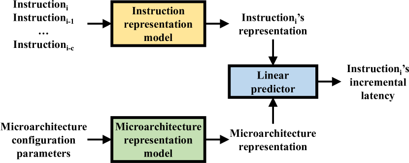
Figure 2: The performance modeling framework to learn generalizable instruction representations.

While it is infeasible to directly learn program representations from billions/trillions of instructions, it is within the capability of today’s ML models to predict the performance of a single instruction and learn its representation. Despite of the extreme complexity of modern processors, the execution and performance of an instruction is mostly affected by hundreds of instructions issued within a relatively narrow window before it (“neighbor” instructions) due to the instruction level parallelism constraint [54]. Capitalizing on this fact, we can construct an ML model to predict the execution latency of an instruction using the properties of itself and neighbors. Note that the performance of an instruction also can be affected by older instructions through caches, etc. Section 3.3 will describe how we capture these long-distance effects through input features.

Figure 2 depicts the notional framework to learn instruction representations. Compared with Figure 1, it replaces the program representation model with the instruction representation model. This model takes the current instruction and previous $c$ instructions as inputs and outputs an instruction representation that is used for performance prediction. Sections 3.3 and 3.4 will introduce more details about the instruction representation model.

Now, we demonstrate how to compose a program representation from those of its executed instructions by carefully designing the PerfVec framework and prediction targets. The first key choice is for the framework to predict the incremental latency of an instruction (shown on the right of Figure 2). It is defined as the time length that an instruction stays active in the processor after all of its predecessors exit. For example, if instructions $I_{0}$, $I_{1}$, and $I_{2}$ retire at 50, 100, and 120 ns respectively, the incremental latency of $I_{2}$ is $120-100=20$ ns. Note that the incremental latency of an instruction may be zero when it retires earlier than its predecessors (this can happen for certain microarchitectures) or at the same time.

To enable the composition of program representations from instruction representations, the second key choice involves selecting the performance predictor to be a linear model without additive biases (the blue box in Figure 2). With these two primary choices, we now prove that the representation of a program can be obtained by summing the representations of all its instructions as follows.

Assume a program executes $n$ instructions in total, and $t_{i}$ and $\bm{R}_{i}$ are the incremental latency and representation of the $i$th instruction. Because the predictor is a linear model, we get $t_{i}=\bm{R}_{i}\ast\bm{M}$, where $\bm{M}$ is the target microarchitecture representation and $\ast$ is the dot product operation. According to the definition of incremental latency, the total execution time $T$ of this program can be calculated by accumulating all incremental latencies:

$$T =\sum_{i=1}^{n}t_{i}=\sum_{i=1}^{n}(\bm{R}_{i}\ast\bm{M})={\leavevmode\hbox to10.97pt{\vbox to10.97pt{\text{[drawing]}}}}\sum_{i=1}^{n}(\sum_{j=1}^{d}(r_{ij}\times m_{j}))$$

$$={\leavevmode\hbox to10.97pt{\vbox to10.97pt{\text{[drawing]}}}}\sum_{j=1}^{d}(\sum_{i=1}^{n}(r_{ij}\times m_{j}))={\leavevmode\hbox to10.97pt{\vbox to10.97pt{\text{[drawing]}}}}\sum_{j=1}^{d}((\sum_{i=1}^{n}r_{ij})\times m_{j})$$

$$={\leavevmode\hbox to10.97pt{\vbox to10.97pt{\text{[drawing]}}}}(\sum_{i=1}^{n}\bm{R}_{i})\ast\bm{M},$$

where $d$ is the representation dimensionality. and employ the definition of dot product, uses the commutativity of sums, and extracts common factors $m_{j}$.

Because $T=(\sum_{i=1}^{n}\bm{R}_{i})\ast\bm{M}$, we may interpret the sum $\sum_{i=1}^{n}\bm{R}_{i}$ as the representation of this program. That is, the program representation is equal to the summation of representations of all its executed instructions, and a program’s total execution time is predicted using the dot product of the program and microarchitecture representations. Notably, this compositional property only holds when the performance predictor is a linear model and the training target is integrable (i.e., the total execution time can be calculated by summing incremental latencies).

Besides enabling compositional representations, our choice of using a linear performance predictor is also justified by previous human-engineered analytical models [23, 52, 49]. Their manually designed equations to calculate execution time share similar forms of dot products of two vectors. One may wonder whether the use of a fixed linear predictor will affect the predictive ability of PerfVec. Fortunately, PerfVec is still capable of capturing the nonlinearity of performance prediction through deep learning-based instruction and microarchitecture representation models.

Table 1: Input features for the instruction representation model.

Category	Features
Static properties	15 operation features (operation type, direct/indirect branch, memory barrier, etc.); indices and categories for 8 source and 6 destination registers
Dynamic behaviors	Execution fault or not (e.g., divide by zero); branch taken or not
Memory access	Stack distances for instruction fetch; stack distances with respect to all data accesses, all loads, and all stores
Branch predictability	Global branch entropy that considers the taken/untaken history of all branches; local branch entropy that considers the history of the current branch

Advantages of Compositional Representations. Our compositional approach that constructs program representations from instruction representations has several key benefits. 1) As all programs can be viewed as different combinations of the same set of instructions (assuming programs are compiled to the same ISA), we only need to train the instruction representation model once. Then, it is generalizable to any program to learn its representation. We call this instruction representation model the foundation model of PerfVec because of its wide applicability, as partially demonstrated in Section 6.

2) Training an instruction representation model is tractable as there are limited instruction types, while the search space is infinitely large when directly training a program representation model (i.e., infinite instruction combinations). 3) Compositional representations enable not only overall but also detailed analysis, such as execution phase analysis demonstrated in Section 6.3. 4) Another plausible property of the proposed approach is the representations of all instructions can be generated in parallel when calculating the representation of a program, which yields a massive amount of parallelism. Modern parallel accelerators, such as GPUs and TPUs, and distributed systems can exploit this parallelism to reduce the time needed to construct a program’s representation.

3.3 Instruction Features

The instruction representation model requires proper input features to learn the performance characteristics of instructions. These features should be sufficient to capture all performance impacts, and they should also be microarchitecture-independent because we want to learn microarchitecture-independent representations.

Table 1 lists all 51 instruction features. Static instruction properties, such as operation types and register indices, are included, as well as microarchitecture-independent dynamic execution behaviors, e.g., whether or not a branch instruction jumps to its target.

The performance of an instruction is also affected by components that have long-lasting states, including caches, translation lookaside buffers, and branch predictors. Traditionally, people use microarchitecture-dependent features (e.g., cache miss number) to model these effects [23, 37], which cannot be applied here because the goal is to learn microarchitecture-independent representations.

Fortunately, several microarchitecture-independent properties have been proposed for memory access and branch prediction analysis, which, in turn, can be used as the input features for the instruction representation model. To model the impact of memory accesses, we use stack distance [21, 8, 43]. The stack distance of an access is defined as the number of unique memory accesses between the current and last accesses to the same address. Intuitively, accesses with longer stack distances are more likely to miss in caches.

To model the branch predictability, we employ branch entropy [60, 19]. In this method, we use 1 to denote a branch taken and 0 for a branch untaken. Thus, the branch taken history can be represented as a sequence of 0s and 1s. Then, an entropy is calculated on this number sequence, called branch entropy. Branches that show more consistent patterns (e.g., always taken or always not taken) have lower entropies and are easier to predict. For example, a branch that always jumps to the target has only 1s in the number sequence. As a result, its branch entropy is 0. The entropies of a branch are calculated both locally (i.e., only use the history of the current branch) and globally (i.e., include the history of other recent branches) for input features.

3.4 Model Architecture

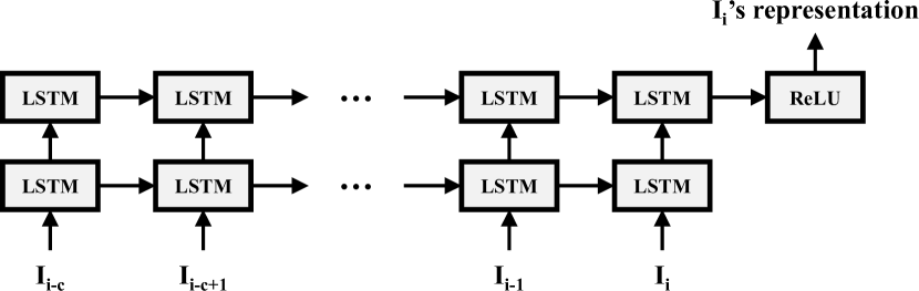
Figure 3: A 2-layer LSTM instruction representation model.

As described in Section 3.2, the input of the foundation model is a sequence of $c+1$ instructions. $c$ determines the number of instructions to look back. Instructions that are closer to the current instruction are likely to have larger impact on its performance, while the impact descends for faraway instructions. In practice, we find that having $c=255$ is enough to capture most impacts of neighbor instructions and considering more instructions is unnecessary. Given that each instruction has 51 features, there are $51\times(255+1)=13056$ input features in total.

Regarding ML model architectures, many have been invented to address sequences. Particularly, we explore convolutional neural network (CNN), long short-term memory (LSTM), gated recurrent unit (GRU), and Transformer models for the foundation model, and train several models from every category as a limited neural architecture search. Our exploration finds a 2-layer 256-dimensional LSTM model performs well enough, and more complex models do not bring significant benefits. Notably, PerfVec users treat the pre-trained foundation model as a black box and its architecture is irrelevant to them as will be shown in Section 6.

Figure 3 depicts the architecture of the 2-layer LSTM model adopted in this work. To learn the representation of the $i$th instruction $I_{i}$, the features of itself and previous $c$ instructions are fed into LSTM blocks in their execution order, with the last instruction $I_{i}$ at the end. Markedly, the rectified linear activation unit (ReLU) is applied before generating the output representation to force instruction representations and consequently program representations to be positive. We find such enforcement results in slightly better prediction accuracy. Note that forcing instruction representations to be positive does not adversely affect the predictive ability of PerfVec as microarchitecture representations can be positive or negative.

The default LSTM model includes 3.3 million parameters in total, which is significantly smaller than recent large models. Because at least 1000 kinds of instructions exist, there are more than $1000^{256}$ possible combinations for the input (a sequence of 256 instructions) of the foundation model. Considering the huge input combination space and the small parameter amount, it is safe to claim that PerfVec does not predict performance by memorizing all possible instruction combinations. Instead, it tries to learn the implicit governing rules of performance modeling.

4 Training the Foundation Model

4.1 Microarchitecture Sampling

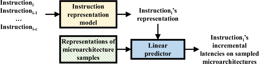
Figure 4: Training a generalizable instruction representation model using microarchitecture sampling and representation reuse.

There are several computational challenges in training the instruction representation model presented in Section 3. As shown in Figure 2, to obtain an instruction representation model, a microarchitecture representation model needs to be jointly trained. However, training a microarchitecture representation model is not trivial because of the huge microarchitecture design space. Describing a conventional microarchitecture requires thousands of parameters. Thus, the microarchitecture design space is larger than $10^{1000}$, and going through even a small portion of this space will result in prohibitively expensive training overheads. In addition, it is also unnecessary to do so as computer architects constantly introduce new microarchitectures. Hence, even if we were able to train a microarchitecture representation model, it likely would not be applicable to future designs.

In this work, we are able to train the instruction representation model without having to train a microarchitecture representation model jointly through microarchitecture sampling. Particularly, we sample a limited number of representative microarchitectures that cover a wide range of the microarchitecture design space and train the instruction representation model by letting it predict the performance on these samples. The hypothesis is that with representative microarchitecture samples, the instruction representation model should be able to learn microarchitecture-independent performance characteristics and generalize to unseen microarchitectures. Section 5.1 will evaluate this hypothesis.

Figure 4 shows the training framework, which replaces the microarchitecture representation model in Figure 2 with a microarchitecture representation table. Dashed models have trainable parameters, and the representations of microarchitecture samples are trained along with the instruction representation model. Of note, there are no parameters in the final linear predictor that performs a simple dot product. In this approach, we only need to train the representations of sampled microarchitectures instead of a microarchitecture representation model that generates representations from configuration parameters.

Training with microarchitecture samples significantly lowers the computational cost and speeds up the convergence because there are fewer parameters to train. As will be introduced soon, we sample 77 microarchitectures in total, resulting in $77\times 256=19.7k$ microarchitecture-related trainable parameters, assuming 256-dimensional representations. Alternatively, assuming to train a basic hypothetical 2-layer neural network microarchitecture representation model with 1000 input parameters and 1000 hidden neurons, there are $1000\times 1000+1000\times 256=1.3$ million parameters to train, which is $\sim 60\times$ bigger. A realistic microarchitecture representation model likely needs to be orders of magnitude larger than this simple model.

4.2 Instruction Representation Reuse

While microarchitecture sampling greatly eases the training burden, the overhead is still extremely high in the conventional training approach where the model predicts the latency of an instruction on one microarchitecture at a time. In this approach, the training time increases linearly with the number of both instructions and sample microarchitectures in the training dataset. Given a training dataset with 737 million instructions and 77 microarchitectures (see Section 4.3), one epoch takes roughly 150 days to go through all 58 billion combinations to train the default 2-layer LSTM using an NVIDIA A6000 GPU. This is prohibitively slow even with multiple GPUs.

Because the instruction representation model is the most computationally intensive part in Figure 4, we propose an efficient training procedure via the reuse of instruction representations. The key fact is that for the same program, its instruction execution trace mostly does not change with the underlying microarchitecture. Capitalizing on this fact, we execute the same program on all sampled microarchitectures to obtain their performance on the same instruction trace. Using these results, given an instruction, we let the model to predict its latencies on all microarchitectures together. During the forward pass of training, we compute the instruction representation once then use it to calculate the incremental latencies on all microarchitectures. During backpropagation, the gradient decent is also performed once on the instruction representation model by averaging gradients with respect to the prediction errors on all microarchitectures. In this way, the expensive forward and backward passes of the instruction representation model are only performed once for each instruction. Instruction representations are reused across microarchitectures.

With instruction representation reuse, we reduce the training time from a linear function to almost irrelevant with respect to the number of microarchitecture samples. In practice, it reduces the training time to roughly two days per epoch from 150 days using one GPU, making the training feasible.

4.3 Dataset

To collect a sufficient dataset to train the foundation model, we leverage the state-of-the-art computer architecture simulator gem5 [12]. Upon the instruction execution trace produced by gem5, we implement a tool to generate the desired input features listed in Table 1 for every instruction, and their incremental latencies as prediction targets.

Microarchitecture. To ensure sufficient coverage of the microarchitecture space, we develop a tool to randomly sample valid gem5 configurations. This tool can alter processor, cache, and memory configurations. For processor configurations, it can vary the processor type (i.e., in-order vs. out-of-order), frequency, pipeline (e.g., fetch stage latency; issue width), execution units (e.g., the number and latency of floating-point multiplication units), and branch predictors. For cache configurations, we can randomly select cache sizes, associativities, latencies, and exclusivity. It can also change the memory type (e.g., DDR4, LPDDR5, GDDR5, or HBM), bandwidth, and frequency. There are hundreds of tunable knobs.

Using this tool, we sample 60 out-of-order and 10 in-order configurations randomly. More out-of-order than in-order processors are sampled, as they are predominant in today’s computer systems and more challenging to model. Together with seven predefined configurations in gem5 (four out-of-order and three in-order), we collect a training dataset with 77 microarchitectures.

Table 2: Benchmarks for ML training and testing.

Type	Training	Testing
INT	525.x264, 531.deepsjeng, 548.exchange2, 557.xz, 999.specrand	500.perlbench, 502.gcc, 505.mcf, 523.xalancbmk
FP	527.cam4, 538.imagick, 544.nab, 549.fotonik3d	507.cactuBSSN, 508.namd, 519.lbm, 521.wrf

Program. We adopt the widely used SPEC CPU2017 benchmark suite [13] to train and test PerfVec. In our gem5 environment, 17 SPEC benchmarks run successfully, and we divide them about evenly for training and testing (shown in Table 2). To ensure fairness, the division is decided based on the benchmark indices: eight benchmarks with smaller indices are used for testing, and the other nine benchmarks are used for training. To collect the training dataset, each training benchmark is simulated using the default test input by 100 million instructions on all 77 microarchitectures. Combining all simulation results, we obtain a training dataset of 2.0 TB.

Note there are no restrictions for the number of programs in the training dataset. Theoretically, all programs in the world can be used in training. We select SPEC CPU2017 benchmarks because of their representativeness. These benchmarks are expected to cover a diverse range of instruction execution scenarios, which should help train generalizable foundation models. Section 5.1 will demonstrate how a larger dataset can help improve generality and accuracy.

4.4 Training Setup

We implement PerfVec’s training and testing framework using PyTorch. The mean squared error between predicted and true latencies is used as the loss function. We adapt the Adam optimizer, where the initial learning rate is set to 0.001 and decayed by $10\times$ every 10 epochs. In total, we train for 50 epochs. A validation set is used to choose the model with the lowest validation loss among all epochs.

We train our models on several GPU servers equipped with 8 NVIDIA A100/A6000 GPUs. With the training optimizations described in Sections 4.1 and 4.2, it takes 12 days to train the default LSTM model on eight A100 GPUs. Notably, PerfVec users, like GPT users, are not burdened with this training overhead because they can directly use the pre-trained foundation model or pre-generated program representations.

5 Evaluation

5.1 Accuracy and Generality

Seen Programs and Seen Microarchitectures. First, we evaluate the prediction accuracy of PerfVec for 9 “seen” programs and 77 “seen” microarchitectures that appear in the training dataset. As discussed in Section 3.4, the 2-layer 256-dimensional LSTM model is adopted as the default foundation model in the following experiments.

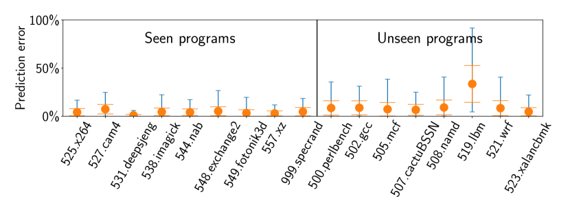
Figure 5: Performance prediction accuracy for seen and unseen programs on seen microarchitectures.

The left side of Figure 5 shows the absolute errors on the predicted execution time of PerfVec compared with gem5 simulation results per seen program. Dots denote the average absolute prediction errors across all 77 seen microarchitectures, orange caps mark standard derivations across microarchitectures, and blue caps mark maximum and minimum errors. We observe the average errors are below 8% for all programs, and the maximum errors are also below 30%, demonstrating PerfVec’s accuracy on seen programs and microarchitectures.

Unseen Programs and Seen Microarchitectures. To achieve the desired generality, it is essential for PerfVec to be able to make accurate predictions on “unseen” programs and microarchitectures that are not available during training. First, we measure the prediction accuracy of PerfVec on unseen programs. To generate the representation of an unseen program, the representations of all its executed instructions are first generated by the pre-trained foundation model. Then, summing them gives the program representation as described in Section 3.2. Together with the representations of 77 seen microarchitectures learned from training, we can predict the performance of unseen programs on seen microarchitectures.

The right side of Figure 5 shows the prediction errors of unseen programs. Although the prediction errors increase compared with those of seen programs, the average errors are below 10% for most unseen programs with 519.lbm as an exception. The main reason why PerfVec generalizes well to most unseen programs is that program representations are composed by instruction representations, and all programs are eventually composed by the same set of instructions, just different combinations. We expect the foundation model to be able to generalize to all possible programs if the training dataset covers enough instruction combination scenarios.

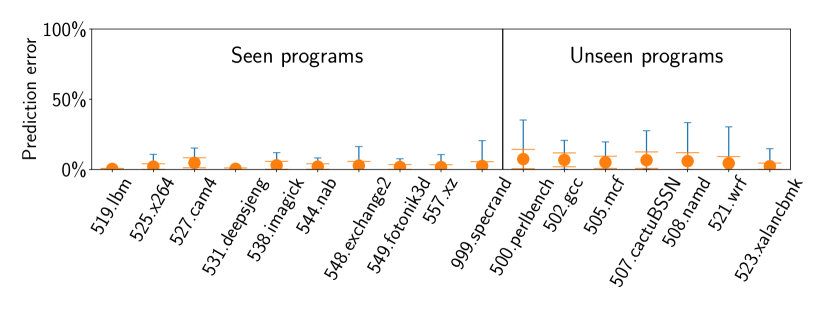
Figure 6: Prediction accuracy on seen microarchitectures after moving 519.lbm to the training dataset.

For the same reason, we hypothesize 519.lbm incurs higher errors because the training dataset lacks sufficient coverage of its instruction combination scenarios. To test this hypothesis, we move 519.lbm to the training dataset and retrain the default model. Figure 6 shows the prediction errors of the model trained on the updated dataset. We observe that the errors of 519.lbm effectively reduce close to zero. Furthermore, the updated model improves the prediction accuracy of other seen and unseen programs, compared with Figure 5. This experiment shows that larger datasets have better instruction combination coverage and improve the generality and accuracy of trained models. The updated model is used in the following experiments.

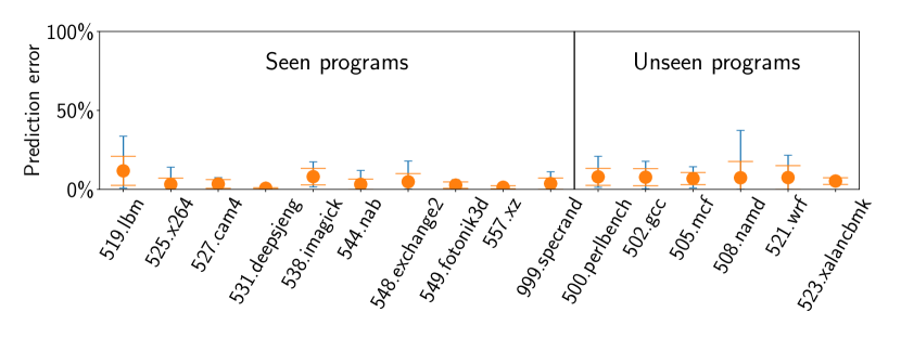
Figure 7: Performance prediction accuracy for seen and unseen programs on unseen microarchitectures.

Unseen Microarchitectures. To test the generality of PerfVec to unseen microarchitectures, we randomly generate 10 microarchitecture configurations that are not used in training and test if PerfVec can accurately predict program performance on these microarchitectures. While it is trivial to obtain the representations of both seen and unseen programs using the pre-trained foundation model, we describe how to obtain the representations of unseen microarchitectures for performance prediction as follows.

Initially, we obtain a small tuning dataset for the target unseen microarchitectures by simulating several seen programs. Then, unseen microarchitecture representations are learned using the framework shown in Figure 4, with an important difference that the yellow instruction representation model is fixed to be the pre-trained foundation model, whose parameters are not updated during training. Only the green microarchitecture representation table is updated in backpropagation to learn the representations of unseen microarchitectures. This process can be viewed as a specific case of fine tuning, which has been applied broadly to tune general-purpose ML models for specific tasks [20].

Figure 7 illustrates the prediction accuracy of all programs on unseen microarchitectures. Because 507.cactuBSSN incurs errors on an unseen microarchitecture in gem5 simulation, it is not included. The average errors across seen and unseen programs are 4.2% and 7.1%, respectively. Individual programs’ errors are comparable with those on seen microarchitectures in Figure 6. Therefore, we conclude that PerfVec generalizes well to unseen microarchitectures.

5.2 Representation Visualization

It is difficult to directly explain the meaning of learned representations due to the black box nature of deep neural networks. However, indirect evidence can be found to verify the meaningfulness of representations produced by PerfVec. We visualize the learned representations of particular microarchitectures and programs for this purpose, by projecting high-dimensional representations into low-dimensional spaces.

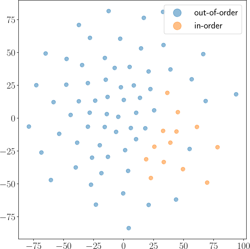
Figure 8: Two-dimensional t-SNE projection of learned microarchitecture representations of various processors.

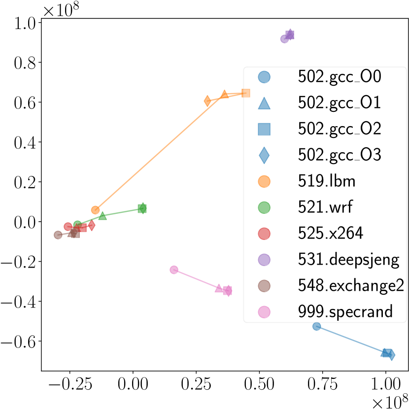
Figure 9: Two-dimensional PCA projection of learned program representations under various compiler optimization levels.

Microarchitecture Representations. Figure 9 shows the t-distributed stochastic neighbor embedding (t-SNE) projection of 77 microarchitectures representations used in the training dataset. Orange and blue dots denote the representations of 13 in-order processors and 64 out-of-order processors, respectively. Because in-order processors work quite differently compared to out-of-order processors, we expect their representations are somehow separate from each other. Indeed, we observe the representations of in-order processors are clustered together, which makes sense due to their similarity, and are away from those of out-of-order processors. This indirectly proves that PerfVec generates meaningful microarchitecture representations.

Program Representations. While it is relatively easy to judge whether two microarchitectures should have similar representations based on their configurations, it is difficult to claim so for two SPEC benchmarks due to their complexity. To demonstrate the foundation model produces meaningful program representations, we design an experiment to visualize the representations of different versions of the same program. Expressly, we visualize the representations of a program under different compiler optimization levels and the distance between them. This is analogous to visualizing the distance between the embeddings of related words, e.g., countries and their capitals [40]. Because the distance in the t-SNE projection is scaled, we adopt the principal component analysis (PCA) to project these program representations.

Figure 9 shows the projected representations of different SPEC programs under four optimization levels of gcc 8.3.1. Cycle, triangle, square, and rhombus markers denote programs compiled using O0, O1, O2, and O3, respectively. Generally, the distance between two representations reflects how similar they are in terms of performance characteristics. Figure 9 includes four seen programs and three unseen programs. The representations of other programs are clustered around (-0.2, 0), and we omit them for clarity. Nevertheless, the observations below also hold for omitted programs.

There are several interesting observations. First, when using higher optimization levels, the representation generally moves to the right on the x axis and to the larger absolute value direction on the y axis (i.e., up when $y>0$ and down when $y<0$). This trend suggests how compiler optimizations transform the representation of a program in general. 519.lbm is an outlier, and its O3 representation is on the left of that of O2. This is due to the challenge to learn an accurate representation of 519.lbm (see Figure 7, where it has the largest error among all programs). Second, the distance between O0 and O1 typically is larger than that between other adjacent optimization levels (i.e., O1—O2, O2—O3). This makes sense because O1 enables essential optimizations that eliminate most unnecessary memory accesses and computations, so there is often a significant performance boost compared with unoptimized programs (i.e., O0). On the other hand, additional optimizations enabled by O3 are considered to have limited effects, so we observe the representations of O2 and O3 are quite similar for most programs. Last, the distance between adjacent optimization levels differs across programs. This reflects the fact that certain compiler optimizations help some programs more than others. For example, 531.deepsjeng has a short distance between O0 and O1, which corresponds to an 8.8% execution time reduction under the ARM Cortex-A7 microarchitecture, while O1 reduces the execution time of 999.specrand by 21.3% on the same microarchitecture, which has a longer O0—O1 distance.

These results demonstrate the meaningfulness of learned program and microarchitecture representations. As a result, besides using program and microarchitecture representations together for performance predictions, they also can be used standalone for quantitative and qualitative analysis.

6 Applications

PerfVec can be applied in many domains where performance modeling plays a critical role. We will illustrate a design space exploration (DSE) case and two program analysis cases.

6.1 Design Space Exploration

DSE Workflow. Leveraging the pre-trained foundation model, we can quickly explore any microarchitecture design space of interest. The proposed microarchitecture DSE procedure works by sampling the microarchitecture design space and simulating several programs to obtain instruction latencies under sampled microarchitectures, which serves as the training dataset. Notably, short simulations can generate a sufficient training set that includes many instructions, and the programs used for training are not necessarily the target programs due to the generality of PerfVec. We train a microarchitecture representation model to take microarchitecture parameters as inputs and output the corresponding microarchitecture representations using the data obtained in the first step. The framework to train the microarchitecture representation model is the same as the one depicted in Figure 2 with the instruction representation model fixed. This process is similar to the method used to obtain unseen microarchitecture representations (described in Section 5.1). The difference is we aim to train a microarchitecture representation model instead of directly getting microarchitecture representations, so that it can explore unseen microarchitecture designs. The training is fast because the pre-trained foundation model does not get updated. The trained microarchitecture representation model can be used to predict the performance of any microarchitecture and program pair with a simple dot product, and the optimal design choice can be found using prediction results.

L1 and L2 Cache Size DSE. As a case study, we explore the design space of L1 data and L2 cache sizes for 17 SPEC programs while using the ARM Cortex-A7 model as the core and fixing other configurations. The L1 data cache size varies from 4 kB to 128 kB, and the L2 cache size varies from 256 kB to 8 MB. Both sizes are constraint to $2^{n}$. Together, there are $6\times 6=36$ configurations.

We assume the objective function to minimize is $(1000+10\times\text{L1\_size\_in\_kB}+\text{L2\_size\_in\_kB})\times\text{execution\_time}$. This objective can be interpreted as finding the optimal cache capacities that minimize the total chip footprint without significant performance loss, for every program. Artificial constants and coefficients are used for illustration purposes without losing generality: A multiplier of 10 is applied to the L1 cache size due to the bigger L1 SRAM cells, and the constant 1000 represents the area overhead of other on-chip components.

We adopt a simple 2-layer multilayer perceptron (MLP) with 4.4 k parameters as the microarchitecture representation model, and its inputs are L1 and L2 cache sizes. We simulate three SPEC programs by 100 million instructions each on 18 sampled microarchitectures to obtain its training dataset.

Results. Out of all 17 target programs, the cache sizes predicted to minimize the objective function by PerfVec are the optimal ones for four of them, among the top two choices for 11 of them, the top three choices for 15 of them, and the top five choices for all. On average, only 3.6% designs outperform the design selected by PerfVec, demonstrating its accuracy.

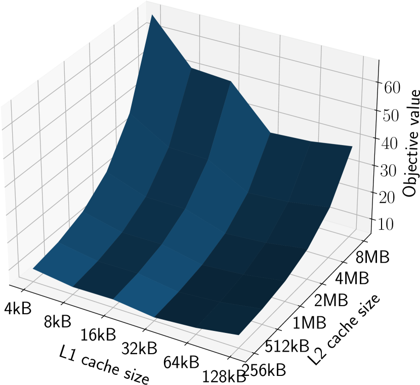
(a) gem5.

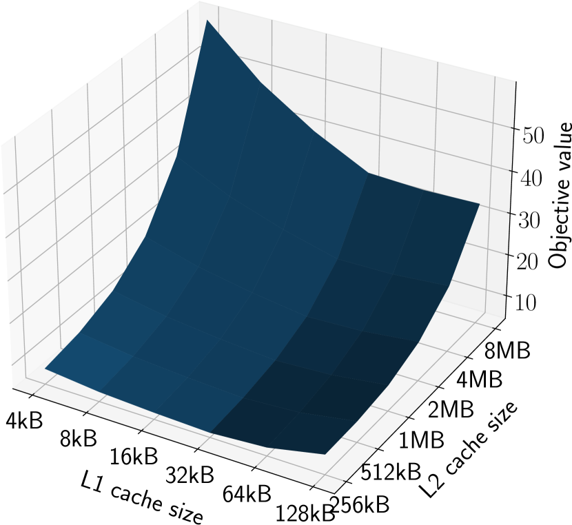
(b) PerfVec.

Figure 10: Objective function values of 508.namd across the cache size search space.

Figure 10 shows the predicted objective function values under various L1 and L2 cache sizes and compares it with those obtained using exhaustive gem5 simulation for 508.namd as an example. While the objective function surfaces of PerfVec and gem5 have similar shapes, an intersting observation is the predicted surface of PerfVec is smoother than that of gem5. This stems from the use of a simple 2-layer MLP microarchitecture representation model, which tends to introduce less nonlinearity to prediction results. Nevertheless, PerfVec correctly projects the trajectories and that a 32 kB L1 data cache works best for all L2 sizes, and large L2 caches do not benefit this benchmark.

PerfVec’s overhead comes from the data collection and the microarchitecture representation model training, and its prediction time is negligible. In total, PerfVec takes 11 hours to accomplish this cache size DSE, including five hours of gem5 simulation for data collection and six hours to train the microarchitecture representation model.

Table 3: Comparison of ML-based DSE methods. Overhead is the time to construct models (hours), and quality is measured by how close the selected design is to the optimal design (smaller is better).

	[28]	[22]	[36]	PerfVec
Overhead	150	84	170	11
Quality	4.4%	4.7%	3.6%	3.6%

Comparison with State-of-the-Art DSE Approaches. Simulation is the most widely used and default method in microarchitecture DSE. Because the time overhead of simulation increases linearly with the number of target programs $\times$ the number of microarchitecture configurations, it is impractical to use simulation for large-scale DSE. In this experiment, to simulate each of 17 programs by one billion instructions on 36 cache configurations, gem5 requires roughly 600 hours, which is about $50\times$ slower than PerfVec. Simulating these programs to the end will require tens of thousands of hours.

Previous research has proposed to train ML-based predictive models using selective simulation results to reduce the simulation workload. Table 3 compares PerfVec with representative ones, including MLP predictors [28], cross-program linear predictors [22], and MLP-based AdaBoost models [36]. These approaches need to simulate every target programs on a significant amount of microarchitecture configurations for model training. To achieve a comparable quality of PerfVec, they require simulating at least 25%, 14%, and 28% of the design space, respectively. These simulations take 84–170 hours, which are 8–15$\times$ of PerfVec’s cost. In the extreme case when sampling the very minimum of a single microarchitecture for every program’s model training, these hardly-trained models make decisions no better than random selection, but still require 17 simulation hours which are longer than PerfVec’s 11 hours.

SimNet is a recent approach that accelerates simulation using ML [37, 44]. It takes 81 hours to finish all simulation of this DSE, which is about $7\times$ faster than gem5 but still $7\times$ slower than PerfVec. Moreover, this is an optimistic cost estimation of SimNet because its training overhead is not considered, which can take days [37].

While the overhead of all above approaches increases with the amount and sizes of target programs, PerfVec has a constant overhead with respect to the program count and sizes thanks to the reusability of program representations. As a result, the speed advantage of PerfVec will be more significant when evaluating more and larger programs.

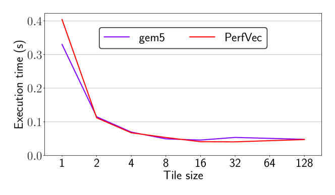
Figure 11: MM performance under various tile sizes.

6.2 Loop Tiling Analysis

The PerfVec framework also can be used for program analysis and optimization. As an example, we devise an experiment to analyze the effect of loop tiling for matrix multiplication (MM). A naive implementation of MM has three nested loops to calculate and accumulate the product of source matrix elements. Our loop tiling implementation blocks all three loops, and a uniform tile size is adopted for simplicity.

Figure 11 compares the execution time of MM generated by gem5 and PerfVec with tile sizes from 1 to 128. The gem5 Cortex-A7 configuration is used as the processor model. The matrix size is $256\times 256$. Overall, the prediction results of PerfVec agree with those of the gem5 simulation. With larger tile sizes, wider vector instructions can be leveraged for better performance, resulting in sharp execution time decrements until the tile size of 8. When a tile exceeds the L1 data cache size, performance degradation is observed due to increasing L1 cache misses, which is insignificant because all matrices fit into the L2 cache. The optimal tile size is 16 under gem5, while PerfVec predicts tile sizes of 16 and 32 having similar and the best performance. Of note, this analysis incurs negligible inference overhead and no training overhead because the pre-trained foundation model is used.

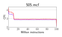
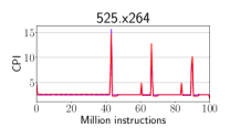
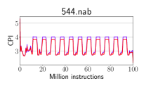
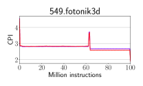
Figure 12: CPI curves generated by gem5 simulation (purple) and PerfVec (red) over 100 million instructions of SPEC programs.

6.3 Phase-level Performance Analysis

Because of the compositional property of instruction representations, we not only can learn the representation of a whole program, but also extract execution phase representations. A phase representation is constructed in a similar way as that of program representations, by summing the representations of all instructions with it. To illustrate this use case, we partition the execution of 100 million instructions into segments of 0.5 million instructions. Then, we extract the representations of these segments to predict their cycles per instruction (CPI).

Figure 12 shows the CPI curves calculated using phase-level representations and compares them to those obtained using gem5 simulation for four programs. A randomly generated microarchitecture configuration in the training dataset is used here. The predicted CPI curves of PerfVec capture the overall performance variations well for all programs, and they thus can help identify potential performance bottlenecks. This observation also holds for other microarchitectures and programs that are not shown in Figure 12 due to the space constraint. In comparison, only expensive simulation can provide such execution details, and existing analytical modeling approaches cannot accomplish it easily because they are not compositional.

7 Related Work and Comparison

Table 4: Comparison with relevant approaches.

Approach	Target	Overhead		Independence
		Training	Prediction	Program	Architecture
ML-based program-specific models [28, 33, 36, 15]	Programs	Slow	Fast	✗	✗
ML-based cross-program models [22, 32]	Programs	Medium slow	Fast	✓	✗
Ithemal [39, 46]	Basic blocks	Fast	Slow	✓	✗
Performance embedding [51]	Loop nests	Medium	Medium	✓	✗
SimNet [37, 44]	(Sub-)Programs	Medium	Medium slow	✓	✗
PerfVec	(Sub-)Programs	Fast	Fast	✓	✓

ML-based Performance Modeling. Ithemal [39] uses LSTM models to predict the execution latency of static basic blocks composed by a few instructions. Using Ithemal as a surrogate model, DiffTune [46] finds simulator parameters that closely resemble a target microarchitecture through gradient decent. These methods are limited to basic blocks rather than programs. Trümper et al.propose to learn the performance embeddings of parallelizable loop nests which are in turn used to guide compiler optimizations [51]. SimNet [37, 44] predicts individual instruction latencies with CNNs given other currently executed instructions. It predicts program performance by simulating all executed instructions.

Ipek et al.propose using neural networks to model the performance of specific programs [28]. Lee et al.formulate nonlinear regression performance models [34, 33, 35]. COAL combines semi-supervised and active learning to train models [15]. ActBoost integrates statistical sampling and active AdaBoost learning to reduce training overhead [36]. To make prediction for unseen programs, two previous methods use simulation results on a reduced set of microarchitecture configurations to combine existing models [22] or as input [32]. Once-for-all trains neural nets to predict the latency and accuracy of a set of neural architectures [14]. Mosmodel [1] predicts the page table walking performance using a multi-input polynomial model. Wu et al.use performance counters to predict GPU performance and power [59]. [57] predicts the performance of certain benchmark suites for Intel CPUs. [38] uses transfer learning to predict the performance of large scale applications based on those of small scale runs. There also has been research on predicting processor performance/power based on those obtained on different types of processors [4, 6, 41] or with varied ISAs [62, 61]. In all approaches above, trained models are bounded to certain programs and/or architectures, which significantly limits their applicability and generality.

Human-engineered Performance Modeling. The Roofline model offers an analytical framework to model the relationship between computation throughputs and memory access intensity [58]. [23] builds an interval-based model to estimate the performance impact of cache misses/branch mispredictions for out-of-order CPUs. [52] proposes a mechanical model that uses microarchitecture-independent program characteristics as inputs. [24] uses backward regression to infer unknown parameters of mechanistic models. The model in [49] convolves application and machine signatures to predict performance. [7] builds program-specific models to predict the performance of large-scale supercomputers. Palm intends to semi-automatically generate performance models through source code annotations [50]. Due to the extreme complexity of modern processors, human-designed analytical models cannot capture execution details and therefore fail to be accurate.

Learning Semantic Representations of Code. Recent research has applied ML techniques developed for NLP to understand the semantics of program code [2]. Building upon BERT [20], CuBERT learns token representations using surrounding tokens as contextual inputs [30], and CodeBERT takes both code and their natural language descriptions into account [25]. [45] proposes to learn program embeddings by mapping program states before execution to those after execution. [56] offers to learn program embeddings using dynamic execution traces (i.e., variable valuations). Extending that work, [55] integrates symbolic execution traces for better precision. To learn LLVM intermediate representation (IR) embeddings, [9] assumes IR instructions that are close in data or control flow have similar semantics, and IR2VEC takes into account data dependency information [53]. Several recent work explores the use of graph neural network (GNN). [3] uses gated GNN on graphs that include both syntactic and semantic information to reason program structures. [48] uses GNNs to learn representations of static assembly code and its execution states on a combined data and control flow graph. ProGraML uses GNNs to learn instruction and code representations for compiler data flow analysis [17].

Research into semantic representations can be used for tasks such as program classification, completion/repair, and similarity detection [26]. These semantic representations cannot be used for performance prediction.

Comparison with State-of-the-Arts. Table 4 compares PerfVec with its most relevant work. For the prediction target, PerfVec is able to predict performance from large-scale programs to fine-grained execution phases as shown in Section 6.3. In contrary, the state-of-the-art instruction-level model Ithemal [39] only deals with basic blocks due to the large token number challenge depicted in Section 3.1, and performance embedding [51] only targets loop nests because of the limitation of GNN.

Regarding overhead, PerfVec incurs less training overhead thanks to its generality, and its prediction is as fast as analytical models with pre-learned representations. Section 6.1 has compared the overhead of various methods in DSE and demonstrated PerfVec’s performance advantages.

Section 6.1 also demonstrates PerfVec’s accuracy against other program-level performance models. We cannot directly compare the accuracy of PerfVec, Ithemal, and performance embedding because the latter two only work for basic blocks and loop nests. Their papers reported the best Pearson correlation coefficients for performance prediction are 0.918 for Ithemal and 0.6 for performance embedding. In comparison, PerfVec achieves a Pearson correlation coefficient of 0.992 even for unseen microarchitectures.

Most importantly, PerfVec is the only model that achieves both program and architecture independence. In summary, PerfVec is a flexable, fast, accurate, and generalizable model.

8 Conclusion

This paper presents PerfVec, a novel ML-based performance modeling framework that exploits deep learning to autonomously separate the performance impact of programs and microarchitectures. PerfVec produces independent and reusable program and microarchitecture representations that can be used for performance modeling and prediction. The approach enabled by PerfVec has general applicability across a broad spectrum of programs and microarchitectures, as well as speed advantages.

References

- [1] Mohammad Agbarya, Idan Yaniv, Jayneel Gandhi, and Dan Tsafrir. Predicting execution times with partial simulations in virtual memory research: why and how. In IEEE/ACM International Symposium on Microarchitecture (MICRO), Global Online Event, October 2020.
- [2] Miltiadis Allamanis, Earl T. Barr, Premkumar Devanbu, and Charles Sutton. A survey of machine learning for big code and naturalness. ACM Comput. Surv., 51(4), jul 2018.
- [3] Miltiadis Allamanis, Marc Brockschmidt, and Mahmoud Khademi. Learning to represent programs with graphs. In International Conference on Learning Representations, 2018.
- [4] Newsha Ardalani, Clint Lestourgeon, Karthikeyan Sankaralingam, and Xiaojin Zhu. Cross-architecture performance prediction (xapp) using cpu code to predict gpu performance. In Proceedings of the 48th International Symposium on Microarchitecture, MICRO-48, page 725–737, New York, NY, USA, 2015. Association for Computing Machinery.
- [5] Vijay Badrinarayanan, Alex Kendall, and Roberto Cipolla. Segnet: A deep convolutional encoder-decoder architecture for image segmentation. IEEE Transactions on Pattern Analysis and Machine Intelligence, 39(12):2481–2495, 2017.
- [6] I. Baldini, S. J. Fink, and E. Altman. Predicting gpu performance from cpu runs using machine learning. In 2014 IEEE 26th International Symposium on Computer Architecture and High Performance Computing, pages 254–261, 2014.
- [7] K. J. Barker, J. Sancho, D. J. Kerbyson, K. Davis, S. Pakin, A. Hoisie, and M. Lang. Using performance modeling to design large-scale systems. Computer, 42(11):42–49, nov 2009.
- [8] Nathan Beckmann and Daniel Sanchez. Modeling cache performance beyond lru. In 2016 IEEE International Symposium on High Performance Computer Architecture (HPCA), pages 225–236, 2016.
- [9] Tal Ben-Nun, Alice Shoshana Jakobovits, and Torsten Hoefler. Neural code comprehension: A learnable representation of code semantics. In S. Bengio, H. Wallach, H. Larochelle, K. Grauman, N. Cesa-Bianchi, and R. Garnett, editors, Advances in Neural Information Processing Systems 31, pages 3588–3600. Curran Associates, Inc., 2018.
- [10] Y. Bengio, P. Simard, and P. Frasconi. Learning long-term dependencies with gradient descent is difficult. IEEE Transactions on Neural Networks, 5(2):157–166, 1994.
- [11] Yoshua Bengio, Aaron Courville, and Pascal Vincent. Representation learning: A review and new perspectives. IEEE Transactions on Pattern Analysis and Machine Intelligence, 35(8):1798–1828, 2013.
- [12] Nathan Binkert, Bradford Beckmann, Gabriel Black, Steven K. Reinhardt, Ali Saidi, Arkaprava Basu, Joel Hestness, Derek R. Hower, Tushar Krishna, Somayeh Sardashti, and et al. The gem5 simulator. SIGARCH Comput. Archit. News, 39(2):1–7, August 2011.
- [13] James Bucek, Klaus-Dieter Lange, and Jóakim v. Kistowski. Spec cpu2017: Next-generation compute benchmark. In Companion of the 2018 ACM/SPEC International Conference on Performance Engineering, pages 41–42, 2018.
- [14] Han Cai, Chuang Gan, Tianzhe Wang, Zhekai Zhang, and Song Han. Once-for-all: Train one network and specialize it for efficient deployment. In International Conference on Learning Representations, 2019.
- [15] Tianshi Chen, Yunji Chen, Qi Guo, Zhi-Hua Zhou, Ling Li, and Zhiwei Xu. Effective and efficient microprocessor design space exploration using unlabeled design configurations. ACM Trans. Intell. Syst. Technol., 5(1), jan 2014.
- [16] Derek Chiou, Dam Sunwoo, Joonsoo Kim, Nikhil A. Patil, William Reinhart, Darrel Eric Johnson, Jebediah Keefe, and Hari Angepat. Fpga-accelerated simulation technologies (fast): Fast, full-system, cycle-accurate simulators. In 40th Annual IEEE/ACM International Symposium on Microarchitecture (MICRO 2007), pages 249–261, 2007.
- [17] Chris Cummins, Zacharias V. Fisches, Tal Ben-Nun, Torsten Hoefler, Michael F P O’Boyle, and Hugh Leather. Programl: A graph-based program representation for data flow analysis and compiler optimizations. In Marina Meila and Tong Zhang, editors, Proceedings of the 38th International Conference on Machine Learning, volume 139 of Proceedings of Machine Learning Research, pages 2244–2253. PMLR, 18–24 Jul 2021.
- [18] Tri Dao, Dan Fu, Stefano Ermon, Atri Rudra, and Christopher Ré. Flashattention: Fast and memory-efficient exact attention with io-awareness. In S. Koyejo, S. Mohamed, A. Agarwal, D. Belgrave, K. Cho, and A. Oh, editors, Advances in Neural Information Processing Systems, volume 35, pages 16344–16359. Curran Associates, Inc., 2022.
- [19] Sander De Pestel, Stijn Eyerman, and Lieven Eeckhout. Linear branch entropy: Characterizing and optimizing branch behavior in a micro-architecture independent way. IEEE Transactions on Computers, 66(3):458–472, 2017.
- [20] Jacob Devlin, Ming-Wei Chang, Kenton Lee, and Kristina Toutanova. Bert: Pre-training of deep bidirectional transformers for language understanding. arXiv preprint arXiv:1810.04805, 2018.
- [21] Chen Ding and Yutao Zhong. Predicting whole-program locality through reuse distance analysis. In Proceedings of the ACM SIGPLAN 2003 Conference on Programming Language Design and Implementation, PLDI ’03, page 245–257, New York, NY, USA, 2003. Association for Computing Machinery.
- [22] Christophe Dubach, Timothy Jones, and Michael O’Boyle. Microarchitectural design space exploration using an architecture-centric approach. In 40th Annual IEEE/ACM International Symposium on Microarchitecture (MICRO 2007), pages 262–271, 2007.
- [23] Stijn Eyerman, Lieven Eeckhout, Tejas Karkhanis, and James E. Smith. A mechanistic performance model for superscalar out-of-order processors. ACM Trans. Comput. Syst., 27(2), may 2009.
- [24] Stijn Eyerman, Kenneth Hoste, and Lieven Eeckhout. Mechanistic-empirical processor performance modeling for constructing cpi stacks on real hardware. In (IEEE ISPASS) IEEE International Symposium on Performance Analysis of Systems and Software, pages 216–226, 2011.
- [25] Zhangyin Feng, Daya Guo, Duyu Tang, Nan Duan, Xiaocheng Feng, Ming Gong, Linjun Shou, Bing Qin, Ting Liu, Daxin Jiang, and Ming Zhou. CodeBERT: A pre-trained model for programming and natural languages. In Findings of the Association for Computational Linguistics: EMNLP 2020, pages 1536–1547, Online, November 2020. Association for Computational Linguistics.
- [26] GitHub. Github copilot · your ai pair programmer. 2022.
- [27] Adolfy Hoisie, Olaf Lubeck, and Harvey Wasserman. Performance and scalability analysis of teraflop-scale parallel architectures using multidimensional wavefront applications. The International Journal of High Performance Computing Applications, 14(4):330–346, 2000.
- [28] Engin Ïpek, Sally A. McKee, Rich Caruana, Bronis R. de Supinski, and Martin Schulz. Efficiently exploring architectural design spaces via predictive modeling. In Proceedings of the 12th International Conference on Architectural Support for Programming Languages and Operating Systems, ASPLOS XII, page 195–206, New York, NY, USA, 2006. Association for Computing Machinery.
- [29] John Jumper, Richard Evans, Alexander Pritzel, Tim Green, Michael Figurnov, Olaf Ronneberger, Kathryn Tunyasuvunakool, Russ Bates, Augustin Žídek, Anna Potapenko, et al. Highly accurate protein structure prediction with alphafold. Nature, 596(7873):583–589, 2021.
- [30] Aditya Kanade, Petros Maniatis, Gogul Balakrishnan, and Kensen Shi. Learning and evaluating contextual embedding of source code. In Hal Daumé III and Aarti Singh, editors, Proceedings of the 37th International Conference on Machine Learning, volume 119 of Proceedings of Machine Learning Research, pages 5110–5121. PMLR, 13–18 Jul 2020.
- [31] Sagar Karandikar, Howard Mao, Donggyu Kim, David Biancolin, Alon Amid, Dayeol Lee, Nathan Pemberton, Emmanuel Amaro, Colin Schmidt, Aditya Chopra, Qijing Huang, Kyle Kovacs, Borivoje Nikolic, Randy Katz, Jonathan Bachrach, and Krste Asanović. Firesim: Fpga-accelerated cycle-exact scale-out system simulation in the public cloud. In Proceedings of the 45th Annual International Symposium on Computer Architecture, ISCA ’18, page 29–42. IEEE Press, 2018.
- [32] Salman Khan, Polychronis Xekalakis, John Cavazos, and Marcelo Cintra. Using predictive modeling for cross-program design space exploration in multicore systems. In 16th International Conference on Parallel Architecture and Compilation Techniques (PACT 2007), pages 327–338, 2007.
- [33] B. C. Lee and D. M. Brooks. Illustrative design space studies with microarchitectural regression models. In 2007 IEEE 13th International Symposium on High Performance Computer Architecture, pages 340–351, 2007.
- [34] Benjamin C. Lee and David M. Brooks. Accurate and efficient regression modeling for microarchitectural performance and power prediction. In Proceedings of the 12th International Conference on Architectural Support for Programming Languages and Operating Systems, ASPLOS XII, page 185–194, New York, NY, USA, 2006. Association for Computing Machinery.
- [35] Benjamin C. Lee, David M. Brooks, Bronis R. de Supinski, Martin Schulz, Karan Singh, and Sally A. McKee. Methods of inference and learning for performance modeling of parallel applications. In Proceedings of the 12th ACM SIGPLAN Symposium on Principles and Practice of Parallel Programming, PPoPP ’07, page 249–258, New York, NY, USA, 2007. Association for Computing Machinery.
- [36] Dandan Li, Shuzhen Yao, Yu-Hang Liu, Senzhang Wang, and Xian-He Sun. Efficient design space exploration via statistical sampling and adaboost learning. In Proceedings of the 53rd Annual Design Automation Conference, DAC ’16, New York, NY, USA, 2016. Association for Computing Machinery.
- [37] Lingda Li, Santosh Pandey, Thomas Flynn, Hang Liu, Noel Wheeler, and Adolfy Hoisie. Simnet: Accurate and high-performance computer architecture simulation using deep learning. Proc. ACM Meas. Anal. Comput. Syst., 6(2), jun 2022.
- [38] Aniruddha Marathe, Rushil Anirudh, Nikhil Jain, Abhinav Bhatele, Jayaraman Thiagarajan, Bhavya Kailkhura, Jae-Seung Yeom, Barry Rountree, and Todd Gamblin. Performance modeling under resource constraints using deep transfer learning. In Proceedings of the International Conference for High Performance Computing, Networking, Storage and Analysis, SC ’17, New York, NY, USA, 2017. Association for Computing Machinery.
- [39] Charith Mendis, Alex Renda, Saman Amarasinghe, and Michael Carbin. Ithemal: Accurate, portable and fast basic block throughput estimation using deep neural networks. In International Conference on Machine Learning, pages 4505–4515. PMLR, 2019.
- [40] Tomas Mikolov, Ilya Sutskever, Kai Chen, Greg S Corrado, and Jeff Dean. Distributed representations of words and phrases and their compositionality. In C.J. Burges, L. Bottou, M. Welling, Z. Ghahramani, and K.Q. Weinberger, editors, Advances in Neural Information Processing Systems, volume 26. Curran Associates, Inc., 2013.
- [41] Kenneth O’neal, Philip Brisk, Ahmed Abousamra, Zack Waters, and Emily Shriver. Gpu performance estimation using software rasterization and machine learning. ACM Trans. Embed. Comput. Syst., 16(5s), September 2017.
- [42] OpenAI. What is the difference between the gpt-4 models?
- [43] Scott Pakin and Patrick McCormick. Hardware-independent application characterization. In 2013 IEEE International Symposium on Workload Characterization (IISWC), pages 111–112, 2013.
- [44] Santosh Pandey, Lingda Li, Thomas Flynn, Adolfy Hoisie, and Hang Liu. Scalable deep learning-based microarchitecture simulation on gpus. In Proceedings of the International Conference on High Performance Computing, Networking, Storage and Analysis, SC ’22. IEEE Press, 2022.
- [45] Chris Piech, Jonathan Huang, Andy Nguyen, Mike Phulsuksombati, Mehran Sahami, and Leonidas Guibas. Learning program embeddings to propagate feedback on student code. In Francis Bach and David Blei, editors, Proceedings of the 32nd International Conference on Machine Learning, volume 37 of Proceedings of Machine Learning Research, pages 1093–1102, Lille, France, 07–09 Jul 2015. PMLR.
- [46] Alex Renda, Yishen Chen, Charith Mendis, and Michael Carbin. Difftune: Optimizing cpu simulator parameters with learned differentiable surrogates. In IEEE/ACM International Symposium on Microarchitecture, 2020.
- [47] A. F. Rodrigues, K. S. Hemmert, B. W. Barrett, C. Kersey, R. Oldfield, M. Weston, R. Risen, J. Cook, P. Rosenfeld, E. Cooper-Balis, and B. Jacob. The structural simulation toolkit. SIGMETRICS Perform. Eval. Rev., 38(4):37–42, mar 2011.
- [48] Zhan Shi, Kevin Swersky, Daniel Tarlow, Parthasarathy Ranganathan, and Milad Hashemi. Learning execution through neural code fusion. In International Conference on Learning Representations, 2020.
- [49] A. Snavely, L. Carrington, N. Wolter, J. Labarta, R. Badia, and A. Purkayastha. A framework for performance modeling and prediction. In SC ’02: Proceedings of the 2002 ACM/IEEE Conference on Supercomputing, pages 21–21, 2002.
- [50] Nathan R. Tallent and Adolfy Hoisie. Palm: Easing the burden of analytical performance modeling. In Proceedings of the 28th ACM International Conference on Supercomputing, ICS ’14, page 221–230, New York, NY, USA, 2014. Association for Computing Machinery.
- [51] Lukas Trümper, Tal Ben-Nun, Philipp Schaad, Alexandru Calotoiu, and Torsten Hoefler. Performance embeddings: A similarity-based transfer tuning approach to performance optimization. In Proceedings of the 37th International Conference on Supercomputing, ICS ’23, page 50–62, New York, NY, USA, 2023. Association for Computing Machinery.
- [52] Sam Van den Steen, Stijn Eyerman, Sander De Pestel, Moncef Mechri, Trevor E. Carlson, David Black-Schaffer, Erik Hagersten, and Lieven Eeckhout. Analytical processor performance and power modeling using micro-architecture independent characteristics. IEEE Transactions on Computers, 65(12):3537–3551, 2016.
- [53] S. VenkataKeerthy, Rohit Aggarwal, Shalini Jain, Maunendra Sankar Desarkar, Ramakrishna Upadrasta, and Y. N. Srikant. Ir2vec: Llvm ir based scalable program embeddings. ACM Trans. Archit. Code Optim., 17(4), dec 2020.
- [54] David W. Wall. Limits of instruction-level parallelism. In Proceedings of the Fourth International Conference on Architectural Support for Programming Languages and Operating Systems, ASPLOS IV, page 176–188, New York, NY, USA, 1991. Association for Computing Machinery.
- [55] Ke Wang and Zhendong Su. Blended, precise semantic program embeddings. In Proceedings of the 41st ACM SIGPLAN Conference on Programming Language Design and Implementation, PLDI 2020, page 121–134, New York, NY, USA, 2020. Association for Computing Machinery.
- [56] Ke Wang, Zhendong Su, and Rishabh Singh. Dynamic neural program embeddings for program repair. In International Conference on Learning Representations, 2018.
- [57] Yu Wang, Victor Lee, Gu-Yeon Wei, and David Brooks. Predicting new workload or cpu performance by analyzing public datasets. ACM Trans. Archit. Code Optim., 15(4), jan 2019.
- [58] Samuel Williams, Andrew Waterman, and David Patterson. Roofline: An insightful visual performance model for multicore architectures. Commun. ACM, 52(4):65–76, apr 2009.
- [59] Gene Wu, Joseph L. Greathouse, Alexander Lyashevsky, Nuwan Jayasena, and Derek Chiou. Gpgpu performance and power estimation using machine learning. In 2015 IEEE 21st International Symposium on High Performance Computer Architecture (HPCA), pages 564–576, 2015.
- [60] Takashi Yokota, Kanemitsu Ootsu, and Takanobu Baba. Potentials of branch predictors: From entropy viewpoints. In Uwe Brinkschulte, Theo Ungerer, Christian Hochberger, and Rainer G. Spallek, editors, Architecture of Computing Systems – ARCS 2008, pages 273–285, Berlin, Heidelberg, 2008. Springer Berlin Heidelberg.
- [61] Xinnian Zheng, Lizy K. John, and Andreas Gerstlauer. Accurate phase-level cross-platform power and performance estimation. In Proceedings of the 53rd Annual Design Automation Conference, DAC ’16, New York, NY, USA, 2016. Association for Computing Machinery.
- [62] Xinnian Zheng, Pradeep Ravikumar, Lizy K John, and Andreas Gerstlauer. Learning-based analytical cross-platform performance prediction. In 2015 International Conference on Embedded Computer Systems: Architectures, Modeling, and Simulation (SAMOS), pages 52–59. IEEE, 2015.