Abstract

Selecting the step size for the Metropolis-adjusted Langevin algorithm (MALA) is necessary in order to obtain satisfactory performance. However, finding an adequate step size for an arbitrary target distribution can be a difficult task and even the best step size can perform poorly in specific regions of the space when the target distribution is sufficiently complex. To resolve this issue we introduce autoMALA, a new Markov chain Monte Carlo algorithm based on MALA that automatically sets its step size at each iteration based on the local geometry of the target distribution. We prove that autoMALA has the correct invariant distribution, despite continual automatic adjustments of the step size. Our experiments demonstrate that autoMALA is competitive with related state-of-the-art MCMC methods, in terms of the number of log density evaluations per effective sample, and it outperforms state-of-the-art samplers on targets with varying geometries. Furthermore, we find that autoMALA tends to find step sizes comparable to optimally-tuned MALA when a fixed step size suffices for the whole domain.

1 INTRODUCTION

The Metropolis-adjusted Langevin algorithm (MALA), introduced by Rossky et al., (1978), is a well-established Markov chain Monte Carlo (MCMC) method for asymptotically obtaining samples from a target distribution $\pi$. As a gradient-based method, MALA often provides better performance than, for example, random-walk Metropolis–Hastings (MH), because gradients direct the sampler to high-density regions in the target distribution. MALA is based on an approximation to overdamped Langevin dynamics, followed by a Metropolis–Hastings correction to account for the approximation.

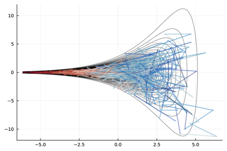
Figure 1: 1000 iterations of autoMALA on Neal’s funnel. Paths between points are coloured according to the automatically selected step size chosen by autoMALA (red for small steps, blue for large steps).

A key challenge in using MALA is that it requires the selection of a step size, $\epsilon$, which controls the level of refinement of the approximation to Langevin dynamics. The dynamics are stated as a stochastic differential equation (SDE). As $\epsilon\to 0$, we perform smaller time updates to our SDE approximation, resulting in a higher acceptance probability of the proposal. This high acceptance rate comes at the expense of slow mixing due to the small step size $\epsilon$. On the other hand, as $\epsilon\to\infty$, more distant moves are generally proposed, at the expense of a fall in the acceptance rate, leading again to slow mixing. There is therefore a tradeoff between the distance that one proposal can reach and the resulting acceptance rates. Extensive work (Roberts and Rosenthal,, 1998; Atchadé,, 2006; Marshall and Roberts,, 2012) has been carried out to derive optimal step sizes that strike a balance for this tradeoff.

The fact that traditional MALA uses a single fixed step size to explore the whole state space makes it inadequate for target densities whose scales and correlations vary across the state space (e.g., the funnel in Fig. 1). To tackle this fundamental limitation, in this work we introduce autoMALA, a new MCMC algorithm based on the Langevin diffusion that dynamically selects an appropriate step size at every MCMC iteration. Crucially, our method ensures that we sample from the correct target distribution even in the presence of this dynamic step size selection. We conduct experiments that establish the desirable properties of autoMALA in terms of the number of time step updates (related to the number of density evaluations) required per effective sample when compared to hand-tuned MALA and NUTS (Hoffman et al.,, 2014). All proofs and experimental details are provided in the supplement.

Related work. There is a large literature devoted to selecting a single optimal step size for MALA. Roberts and Rosenthal, (1998) use scaling limits to argue that the step size should be set to obtain an average acceptance rate of $0.574$. More recently, adaptive MCMC methods (Atchadé and Rosenthal,, 2005) have been developed specifically for MALA (Atchadé,, 2006; Marshall and Roberts,, 2012), which adjust the step size on the fly to target the $0.574$ rate while preserving the correct invariant distribution. Alternatively, general-purpose tuning procedures for gradient-based MCMC (see e.g. Coullon et al.,, 2023) tune hyperparameters by directly minimizing a divergence between the target and the sample-based distribution. Furthermore, Livingstone and Zanella, (2022) propose a novel MH algorithm that exhibits the same dimensional scaling as MALA while being more robust to the choice of step size. Still, the fact that these algorithms depend on a fixed step size makes them inappropriate for targets with varying local geometry.

In the Hamiltonian Monte Carlo (HMC) literature there is comparatively more attention on dynamic, automatic selection of proposal length scale via selection of the number of steps $L$ between momentum refreshments (Hoffman et al.,, 2014). However, $n$ steps of doubling the trajectory length $L$ takes compute time proportional to $2^{n}$, whereas $n$ steps of step size doubling in the autoMALA algorithm has a cost proportional to $n$. Therefore, for target distributions with sufficiently variable geometries, dynamic step size selection is preferable to dynamic trajectory length selection, as we also demonstrate empirically. In this vein, several approximate Monte Carlo algorithms—i.e, which do not preserve the distribution $\pi$—based on variable step size integrators of Hamiltonian dynamics have been proposed (see e.g. Kleppe,, 2022). However, our focus is on asymptotically exact MCMC; we therefore exclude such approximate algorithms from our analyses.

Kleppe, (2016) is one of the few works that tackles $\pi$-invariant dynamic step size selection. However, its step size selection routine (Algorithm 2 in Kleppe, (2016)) does not take into account the direction of the proposal and may not terminate in general. Modi et al., (2023) also proposes a dynamic step size algorithm, based on the delayed-rejection method (Tierney and Mira,, 1999, Sec. 5). Because of this, the algorithm in Modi et al., (2023) requires setting a priori a maximum number of proposed step sizes, whereas autoMALA does not. Finally, Girolami and Calderhead, (2011) study MALA and HMC with position-dependent preconditioning (a randomized “mass matrix”), which provides an alternative way of making an informed selection of the step size. Nishimura and Dunson, (2016) further extend this idea by employing explicit variable step size integrators. However, these methods have a compute cost per leapfrog step that scale superlinearly in the number of dimensions. While they provide improved mixing, in medium or high-dimensional problems these gains are often not sufficient to counteract exploding cost per step, and therefore these methods have limited or no empirical advantages in high-dimensional problems (Girolami and Calderhead,, 2011). In contrast, the cost of one autoMALA step scales linearly with dimension.

2 BACKGROUND

Let $\pi$ be a probability distribution of interest on $\mathbb{R}^{d}$, which we assume can be written as

$$\pi(x):=\frac{\gamma(x)}{\int_{\mathbb{R}^{d}}\gamma(u)\,\mathrm{d}u},$$ (2)

where $\gamma$ can be evaluated pointwise and is continuously differentiable. Consider the following special case of the stochastic differential equation known as the Langevin diffusion (Roberts and Stramer,, 2002):

$$\mathrm{d}X_{t}=\frac{1}{2}C\nabla\log\gamma(X_{t})\mathrm{d}t+C^{1/2}\mathrm{d}W_{t}.$$ (3)

Here, $\{W_{t}\}_{t\geq 0}$ is a Wiener process and $C$ is any user-defined positive-definite matrix. Under certain regularity conditions (Roberts and Stramer,, 2002), the solution $\{X(t)\}_{t\geq 0}$ of Eq. 3 is ergodic and has $\pi$ as its stationary distribution. We can build a discrete-time Markov chain $\{\tilde{x}_{n}\}_{n\in\mathbb{N}}$ approximating $\{X(t)\}_{t\geq 0}$ via the Euler–Maruyama discretization, with the update

$$\tilde{x}^{\prime}|\tilde{x}\sim\mathcal{N}\left(\tilde{x}+\frac{h}{2}C\nabla\log\gamma(\tilde{x}),\,hC\right),$$ (4)

where $h>0$ denotes a step size. This approximation is known as the unadjusted Langevin algorithm (ULA). ULA with a fixed step size $h>0$ does not in general admit $\pi$ as a stationary distribution.

MALA is a modification of ULA that restores the desired stationary distribution by using ULA as a proposal within a Metropolis–Hastings scheme. Concretely, at any point $x\in\mathbb{R}^{d}$, MALA selects the next state $x^{\prime}$ to be the ULA update $\tilde{x}^{\prime}|x$ with probability

$$\min\left\{1,\frac{\gamma(\tilde{x}^{\prime})\mathcal{N}\left(x\mid\tilde{x}^{\prime}+\frac{h}{2}C\nabla\log\gamma(\tilde{x}^{\prime}),\,hC\right)}{\gamma(x)\mathcal{N}\left(\tilde{x}^{\prime}\mid x+\frac{h}{2}C\nabla\log\gamma(x),\,hC\right)}\right\},$$ (5)

and otherwise sets $x^{\prime}=x$, where $\mathcal{N}(\cdot|\mu,\,\Sigma)$ is the density of a $\mathcal{N}(\mu,\Sigma)$ distribution. This modification makes $\{x_{n}\}_{n\in\mathbb{N}}$ an ergodic, $\pi$-reversible, and $\pi$-invariant Markov chain under appropriate conditions.

We can reframe MALA as HMC with a single leapfrog step (Eq. 7) of size $\epsilon=h^{1/2}$ and positive definite mass matrix $M=C^{-1}$ (Neal,, 2011, §5.2). Our exposition of autoMALA exploits this fact. We expand the space from $\mathbb{R}^{d}$ to $\mathbb{R}^{2d}$ and augment the target density:

$$\pi_{\mathrm{HMC}}(x,p):=\pi(x)\cdot\mathcal{N}(p\mid 0,\,M).$$ (6)

Note that $x$ and $p$ are independent, and the $x$ marginal is the target distribution of interest $\pi$. The MALA proposal is equivalent to drawing $p\sim\mathcal{N}(0,M)$ and then applying a map $L_{\epsilon}:\mathbb{R}^{2d}\to\mathbb{R}^{2d}$ consisting of a single leapfrog step of size $\epsilon>0$ and a momentum flip:

$$p_{\nicefrac{{1}}{{2}}}^{\prime} =p+\frac{\epsilon}{2}\nabla\log\gamma(x)$$ (7)

$$x^{\prime} =x+\epsilon M^{-1}p^{\prime}_{\nicefrac{{1}}{{2}}}$$ (8)

$$\check{p} =p^{\prime}_{\nicefrac{{1}}{{2}}}+\frac{\epsilon}{2}\nabla\log\gamma(x^{\prime})$$ (9)

$$p^{\prime} =-\check{p}.$$ (10)

The map $L_{\epsilon}$ is an involution, i.e., $L_{\epsilon}=(L_{\epsilon})^{-1}$, and is volume preserving, $|\det\nabla L_{\epsilon}|=1$ (see, e.g., Neal,, 2011); we use these facts and results from Tierney, (1998) in the analysis of autoMALA. The proposal $(x^{\prime},p^{\prime})$ is then accepted with probability

$$\alpha((x,p),(x^{\prime},p^{\prime})):=\min\left\{1,\frac{\gamma(x^{\prime})\mathcal{N}(p^{\prime}\mid 0,M)}{\gamma(x)\mathcal{N}(p\mid 0,M)}\right\}.$$ (11)

We finish this section by noting an important motivation for autoMALA: it is necessary to determine a step size $\epsilon$ for MALA that appropriately balances the acceptance rate with fast exploration of the state space. However, to account for different length scales of $\pi$ in different regions of state space, this tradeoff should be made at each iteration, dependent on the current position $(x,p)$ in the state space. Our proposed sampler, autoMALA, does exactly this: autoMALA adapts $\epsilon$ “on the fly” as a function of the current state, and is carefully constructed to ensure that we still asymptotically obtain samples from the correct target distribution $\pi$.

3 AUTOMALA

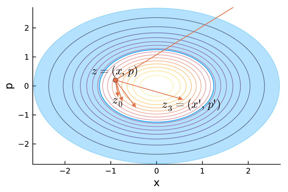
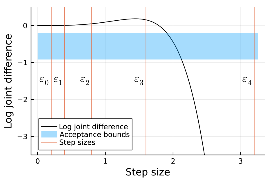
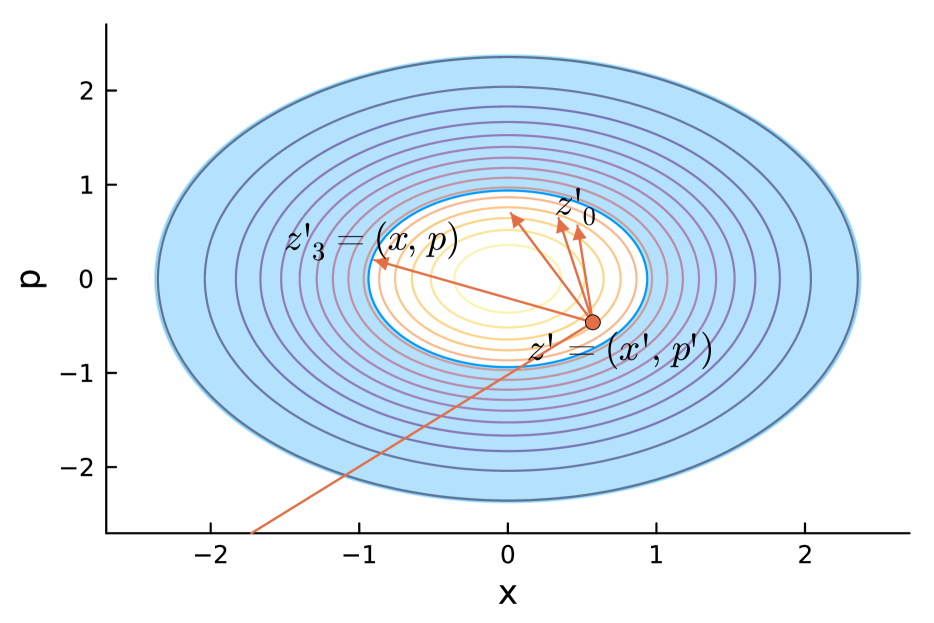
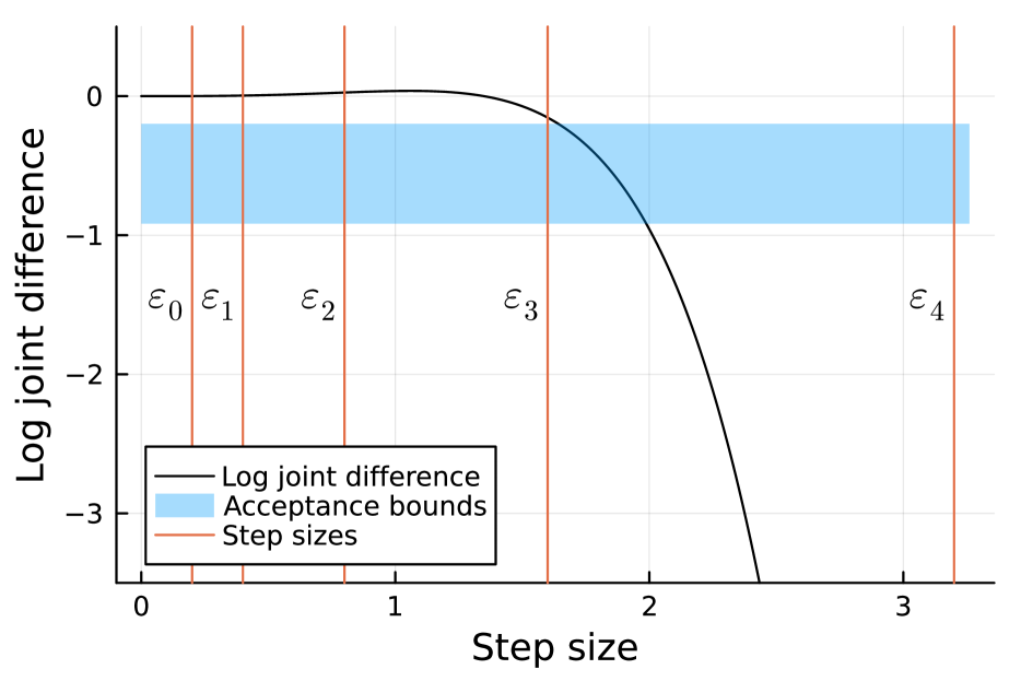
Figure 2: The autoMALA step size selection procedure on a standard univariate normal distribution. Both figures illustrate the phase space for $(x,p)$. In the figure, $z_{j}=L_{\epsilon_{\text{init}}\cdot 2^{j}}(x,p)$ and $z^{\prime}_{j}=L_{\epsilon_{\text{init}}\cdot 2^{j}}(x^{\prime},p^{\prime})$, whereas $z$ and $z^{\prime}$ denote $(x,p)$ and $(x^{\prime},p^{\prime})$, respectively. Similarly, $\epsilon_{j}=\epsilon_{\text{init}}\cdot 2^{j}$. Top (proposal phase): Values of $a,b$ are drawn. The initial density ratio is larger than $b$ and the step size is doubled until the first time we exit the acceptance region (orange arrows). The state just before exiting is proposed. Bottom (reversibility check): The same values of $a,b$ are kept, but a new acceptance region is drawn relative to $(x^{\prime},p^{\prime})$. The number of doublings is the same in both the forward and reverse directions, and we pass the reversibility check. When the initial step size is too large, a similar approach is taken (with the difference of Line 18 instead of Line 16 in Algorithm 2).

autoMALA, at a high level, can be thought of as MALA with an automatic step size selection procedure, followed by corrections to ensure that $\pi$ is invariant. One application of the autoMALA kernel consists of:

1. State augmentation: Sample a momentum $p\sim\mathcal{N}(0,M)$ and two thresholds $a$ and $b$ uniformly from $\Delta:=\{(a,b)\in(0,1)^{2}:a<b\}$. Let $s=(x,p,a,b)\in\mathbb{R}^{2d}\times\Delta$ denote the augmented state.

2. MALA proposal with step size selection: Start at an initial step size guess, $\epsilon_{\text{init}}>0$. Let $r_{\text{init}}$ be the density ratio of the leapfrog proposal $L_{\epsilon_{\text{init}}}(x,p)$. If $r_{\text{init}}\in(a,b)$, keep $\epsilon_{\text{init}}$. If $r_{\text{init}}\leq a$, halve the step size until the ratio is strictly above $a$. Otherwise, if $r_{\text{init}}\geq b$, double the step size until the ratio is strictly less than $b$, and then halve it once. Denote the step size selection function $\epsilon(s,\epsilon_{\text{init}})$.

3. Reversibility check: Let $s^{\prime}=(x^{\prime},p^{\prime},a,b)$ and consider the step size selected from $s^{\prime}$, namely $\epsilon^{\prime}=\epsilon(s^{\prime},\epsilon_{\text{init}})$. If $\epsilon\neq\epsilon^{\prime}$, we remain at $x$. This so-called “reversibility check”—akin to Neal, (2003, Fig. 6)—is essential to keeping the target $\pi$-invariant.

4. Metropolis–Hastings: If the reversibility check passes, apply the MALA Metropolis–Hastings correction, with probability given by Eq. 11.

The first key feature of autoMALA that distinguishes it from standard MALA is the step size selection in Step 2. Drawing the acceptance thresholds $a,b$ uniformly generally keeps the acceptance probability bounded away from the extremes (0 and 1), as desired, without needing to specifically tune their values. For a given pair of thresholds $a<b$, if the initial acceptance ratio is too low relative to $a$ ($\epsilon_{\text{init}}$ too large), we make the steps more conservative by successively halving $\epsilon$ until the ratio is above $a$ (although not necessarily below $b$). If instead the initial acceptance ratio is too high relative to $b$ ($\epsilon_{\text{init}}$ too small), we make the steps more aggressive by successively doubling $\epsilon$ until the ratio is below $b$ (although not necessarily above $a$), and then halving the step size once (Line 16 in Algorithm 2). Note that the asymmetry in these two cases is crucial. Without the final halving, the reversibility check would always fail in the doubling sub-case. To see this, compare the value $\ell$ (Line 14 in Algorithm 2) for the last iteration $j^{*}$ of $\epsilon(s,\epsilon_{\text{init}})$ to the value $\ell^{\prime}$ at iteration $j=j^{*}$ of $\epsilon(s^{\prime},\epsilon_{\text{init}})$. From Line 14, $\ell=-\ell^{\prime}$. Moreover, since $\ell$ comes from the last iteration, by Line 15, $\ell<\log(b)$, and since $b\in(0,1)$, that implies $\ell<0$ so $\ell^{\prime}>0>\log(b)$. Hence $\epsilon(s^{\prime},\epsilon_{\text{init}})$ would generally not terminate at that iteration without the final halving. The same argument does not apply to the halving sub-case, as it is possible to have $\ell>\log(a)$ and $-\ell>\log(a)$ simultaneously.

Another key feature of autoMALA is the reversibility check in Step 3. To understand the basis for this check, let $A$ be the region of the augmented state space $\mathcal{S}=\mathbb{R}^{2d}\times\Delta$ where the reversibility check succeeds, (both the forward and reverse step sizes are the same). Then $A$ is precisely the subset on which the autoMALA proposal is an involution. Hence, autoMALA preserves $\bar{\pi}$ on $A$ when combined with the Metropolis–Hastings correction in Step 4 (Tierney,, 1998). On the complement $A^{c}$, autoMALA is the identity, and so it preserves $\bar{\pi}$ there, as well. Because autoMALA never proposes a state in $A^{c}$ from one in $A$ and vice versa, autoMALA keeps $\bar{\pi}$ invariant on all of $\mathcal{S}$.

Finally, in practice, the step size selection and reversibility check should operate on the integer exponent $j$ of the step size $\epsilon_{\text{init}}\cdot 2^{j}$, instead of the floating point step size itself, so that the reversibility checks do not suffer from floating point errors. This is the reason why Algorithm 2 returns the integer number of doublings as well as the step size.

1:Initial state $x_{0}$, number of iterations $T$, initial step size $\epsilon_{\text{init}}$, preconditioning matrix $\hat{\Sigma}$, number of unadjusted burn-in iterations per round $t_{\text{unadj}}$ (default: $t_{\text{unadj}}=1$)

2:for $t$ in 1, 2, …, $T$ do

3:     $\eta\leftarrow{\mathrm{Beta}}_{01}(1,1,1/2,2/3)$

4:      $\triangleright$ form random preconditioning matrix

5:     $(\hat{\Sigma}_{\text{AM}})_{i,i}^{-1/2}=\eta\hat{\Sigma}_{i,i}^{-1/2}+(1-\eta)$

6:     $p\leftarrow\mathcal{N}(0_{d},\hat{\Sigma}_{\text{AM}}^{-1})$ $\triangleright$ sample momentum

7:     $(u_{1},u_{2})\leftarrow U([0,1]^{2})$

8:      $\triangleright$ soft bounds for acceptance ratio

9:     $(a,b)\leftarrow(\min\{u_{1},u_{2}\},\max\{u_{1},u_{2}\})$

10:     $s\leftarrow(x_{t-1},p,a,b)$

11:     $\epsilon,j\leftarrow\epsilon(s,\epsilon_{\text{init}})$

12:     $s^{\prime}\leftarrow(L_{\epsilon}(x_{t-1},p),a,b)$ $\triangleright$ proposed state

13:     $\epsilon^{\prime},j^{\prime}\leftarrow\epsilon(s^{\prime},\epsilon_{\text{init}})$

14:     $\alpha\leftarrow 1\wedge\bar{\pi}(s^{\prime})/\bar{\pi}(s)$ $\triangleright$ see Section 3.3

15:     $U\leftarrow U[0,1]$

16:     if $t\leq t_{\text{unadj}}$ or $(j=j^{\prime}$ and $U\leq\alpha)$ then

17:         $x_{t}\leftarrow x^{\prime}$ $\triangleright$ accept

18:     else

19:         $x_{t}\leftarrow x_{t-1}$ $\triangleright$ reject

20:     end if

21:     $\epsilon_{t}\leftarrow(\epsilon+\epsilon^{\prime})/2$

22:end for

23:return $\{(x_{t},\epsilon_{t})\}_{t=1}^{T}$

Algorithm 1 autoMALA$(x_{0},T,\epsilon_{\text{init}},\hat{\Sigma},t_{\text{unadj}})$

1:state $s=(x,p,a,b)$, initial step size $\epsilon_{\text{init}}$.

2:$\epsilon\leftarrow\epsilon_{\text{init}}$

3:$s^{\prime}\leftarrow(L_{\epsilon}(x,p),a,b)$

4:$\ell\leftarrow\log\bar{\pi}(s^{\prime})-\log\bar{\pi}(s)$

5:$\delta\leftarrow\mathds{1}\{\ell\geq\log(b)\}-\mathds{1}\{\ell\leq\log(a)\}$

6:$j=0$ $\triangleright$ number of doublings/halvings

7:if $\delta=0$ then

8:     return $\epsilon_{\text{init}}$

9:end if

10:while true do

11:     $\epsilon\leftarrow\epsilon\cdot 2^{\delta}$

12:     $j\leftarrow j+\delta$

13:     $s^{\prime}\leftarrow(L_{\epsilon}(x,p),a,b)$

14:     $\ell\leftarrow\log\bar{\pi}(s^{\prime})-\log\bar{\pi}(s)$

15:     if $\delta=1$ and $\ell<\log(b)$ then

16:         return $\epsilon/2,j-1$ $\triangleright$ See Section 3

17:     else if $\delta=-1$ and $\ell>\log(a)$ then

18:         return $\epsilon,j$

19:     end if

20:end while

Algorithm 2 Step size selector $\epsilon(s,\epsilon_{\text{init}})$

3.1 Round-based tuning

The autoMALA sampler described above chooses an appropriate step size $\epsilon$ at any given point $(x,p)$ in the state space. The computational cost of the step size selection procedure increases logarithmically in the gap between $\epsilon_{\text{init}}$ and the selected step $\epsilon$. To decrease this cost, we use a simple round-based approach to tuning $\epsilon_{\text{init}}$ (Algorithm 3). During tuning round $r$ we perform $T_{r}=2^{r}$ iterations of autoMALA. In the first tuning round, we use $\epsilon_{\text{init}}=1$. At the end of the $r^{\text{th}}$ tuning round, we obtain the average step size used during that tuning round; this then becomes the initial step size $\epsilon_{\text{init}}$ used in the $r+1^{\text{th}}$ tuning round.

Additionally, MALA and autoMALA can perform better with preconditioning, i.e. a positive definite matrix $C\neq I_{d}$ in Eq. 3 (equivalently written as a mass matrix $M=C^{-1}$). We obtain an appropriate preconditioner as a by-product of our round-based adaptive scheme. Our approach is motivated by multivariate normal target distributions with covariance matrix $\Sigma$, where the choice $C=M^{-1}=\Sigma$ is recommended (Neal,, 2011), but to avoid matrix operations with cost superlinear in $d$, it is customary to use a diagonal matrix with entry $(i,i)$ given by the marginal variance of component $i$, $\hat{\Sigma}_{i,i}=\widehat{\operatorname{Var}}[x^{(i)}]$. To improve the robustness of the diagonal matrix approach—which is prone to errors even in the Gaussian setting (Hird and Livingstone,, 2023)—at each step we perform the random interpolation $(\hat{\Sigma}_{\text{AM}})_{i,i}^{-1/2}=\eta\hat{\Sigma}_{i,i}^{-1/2}+(1-\eta)$, with $\eta$ sampled independently from a zero-one-inflated beta distribution, denoted as ${\mathrm{Beta}}_{01}(\tilde{\alpha},\tilde{\beta},p,m)$, for some values of $\tilde{\alpha},\tilde{\beta}>0$ and $p,m\in[0,1]$. Here, ${\mathrm{Beta}}_{01}(\tilde{\alpha},\tilde{\beta},p,m)$ denotes a random variable that is distributed according to ${\mathrm{Bern}}(p)$ with probability $m$ and ${\mathrm{Beta}}(\tilde{\alpha},\tilde{\beta})$ with probability $1-m$. In our experiments, we use $\tilde{\alpha}=\tilde{\beta}=1$, $p=1/2$, and $m=2/3$ so that each of the two endpoints $\{0,1\}$ and the interval $(0,1)$ all have an equal chance ($1/3$) of being selected (see Section B.8 for an experimental validation of this approach).

Note that our round-based procedure does not introduce additional tuning parameters, and plays well with other round-based algorithms such as non-reversible parallel tempering, described in Syed et al., (2021) and implemented in Surjanovic et al., (2023).

1:Initial state $x_{0}$, number of rounds $R$, number of unadjusted burn-in iterations per round $t_{\text{unadj}}$ (default: $t_{\text{unadj}}=1$)

2:$\epsilon_{\text{init}}=1$

3:$\hat{\Sigma}\leftarrow I_{d}$

4:for $r$ in 1, 2, …, $R$ do

5:     $T\leftarrow 2^{r}$

6:     $\{(x_{t},\epsilon_{t})\}_{t=1}^{T}\leftarrow\texttt{autoMALA}(x_{0},T,\epsilon_{\text{init}},\hat{\Sigma},t_{\text{unadj}})$

7:     $\epsilon_{\text{init}}\leftarrow T^{-1}\sum_{t=1}^{T}\epsilon_{t}$

8:     $x_{0}\leftarrow x_{T}$

9:     $\hat{\Sigma}\leftarrow\text{diag}\left(\widehat{\operatorname{Var}}[x_{t}^{(1)}]_{t=1}^{T},\ldots,\widehat{\operatorname{Var}}[x_{t}^{(d)}]_{t=1}^{T}\right)$

10:end for

11:return $\{x_{t}\}_{t=1}^{T}$

Algorithm 3 Round-based autoMALA

3.2 Unadjusted burn-in

Empirically, the reversibility check succeeds with high probability at stationarity in all cases investigated. However, we have also observed situations where an arbitrary initialization yields a near-zero success probability. As a result, we skip the reversibility check and the Metropolis–Hasting rejection step for a constant number of iterations $t_{\text{unadj}}=1$ at the beginning of each round. Empirically we find that this step helps avoid the sampler getting stuck at a bad initial point.

3.3 Theoretical results

In this section we establish that the step size selection algorithm given by Algorithm 2 terminates almost surely (Theorem 3.3) and that autoMALA has the correct invariant distribution $\bar{\pi}$ (Theorem 3.4). The proofs of these theoretical results can be found in the supplementary material. In what follows, we introduce some regularity conditions on the target distribution $\pi$. For a vector $x\in\mathbb{R}^{d}$, let $\lvert x\rvert$ be its Euclidean norm.

Assumption 3.1.

(Smoothness) $\pi$ is twice continuously differentiable on $\mathbb{R}^{d}$.

Assumption 3.2.

(Tails) $\lim_{\lvert x\rvert\to\infty}\pi(x)=0$.

To analyze the autoMALA algorithm, it will be useful to define the augmented density

$$\macc@depth\char 1\relax\frozen@everymath{\macc@group}\macc@set@skewchar\macc@nested@a 111{}(s):=2\pi(x)\cdot\mathcal{N}(p\mid 0,M)\cdot\mathds{1}_{\Delta}(a,b)$$

where $\mathds{1}_{\Delta}(\cdot)$ is the indicator for the set $\Delta$.

Our first result confirms that the step size selection (Algorithm 2) terminates almost surely. For $s\in\mathcal{S}$ and $\epsilon_{\text{init}}>0$, we define $\tau(s,\epsilon_{\text{init}})\geq 1$ to be the number of iterations of the while loop in Algorithm 2.

Theorem 3.3.

(Step size selector termination) Let $\epsilon_{\text{init}}>0$ and suppose that $\pi$ satisfies Assumption 3.1 and Assumption 3.2. Then, $\tau(s,\epsilon_{\text{init}})<\infty$ $\bar{\pi}$-a.s.

We now formally state the $\pi$-invariance property of autoMALA. Suppressing $\epsilon_{\text{init}}$ in the notation, define $L_{\epsilon}(s)=(L_{\epsilon}(x,p),a,b)$, $T(s)=L_{\epsilon(s)}(s)$ and the region $A\subset\mathcal{S}$ where the reversibility check succeeds, $A=\{s\in\mathcal{S}:\epsilon(s)=\epsilon\circ T(s)\}$. Define the deterministic proposal

$$Q_{\mathrm{AM}}(s)=T(s)\mathds{1}_{A}(s)+s\mathds{1}_{A^{c}}(s),$$ (12)

from which we construct the autoMALA kernel

$$K_{\textrm{AM}}(s,\mathrm{d}s^{\prime}) =(1-\alpha(s))\delta_{s}(\mathrm{d}s^{\prime})+\alpha(s)\delta_{Q_{\mathrm{AM}}(s)}(\mathrm{d}s^{\prime})$$ (13)

$$\alpha(s) =\min\left\{1,\frac{\bar{\pi}(Q_{\mathrm{AM}}(s))}{\bar{\pi}(s)}\right\}.$$ (14)

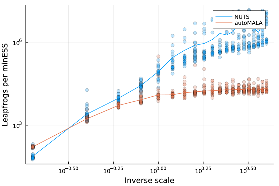
Figure 3: Comparison of autoMALA and NUTS on Neal’s funnel with a varying scale parameter for 20 different seeds. Bold curves indicate averages across seeds. Geometries increase in difficulty from left to right. Left to right: Number of leapfrog evaluations per 1000 minESS (lower is better), estimated mean of the first marginal (exact mean is 0), estimated variance of the first marginal (exact variance is 9).

Theorem 3.4.

(Invariance) Under Assumption 3.1 and Assumption 3.2, for any measurable $B\subset\mathcal{S}$,

$$\int\bar{\pi}(\mathrm{d}s)K_{\mathrm{AM}}(s,B)=\bar{\pi}(B).$$ (15)

Notice that Algorithm 1 is a deterministic composition of $K_{\mathrm{AM}}$ with a block Gibbs update on $p,a,b$, and therefore is $\bar{\pi}$-invariant as a corollary of Theorem 3.4.

Regarding irreducibility, it does not appear straightforward to show that autoMALA can visit any $x$ state after only a single step, unlike MALA. However, we conjecture that autoMALA can still visit any $x$ state after multiple steps under reasonable conditions, which we leave as an open problem. Additionally, one can easily guarantee irreducibility—if desired—by mixing autoMALA with another kernel known to be irreducible. For example, using the mixture $\lambda K_{\text{AM}}+(1-\lambda)K_{\text{MALA}}$, where $K_{\text{MALA}}$ is a MALA transition kernel and $0<\lambda<1$, leads to an irreducible sampler. Of course, $\lambda$ should be chosen close to one in order to retain the adaptive benefits of autoMALA.

4 EXPERIMENTS

In this section, we present experiments that investigate the performance of autoMALA on targets with varying geometry and increasing dimension, as well as the convergence behaviour of the initial step size. We compare autoMALA against the locally adaptive sampler NUTS (Hoffman et al.,, 2014), as well as standard MALA, which is a non-adaptive method. We refer readers to the supplementary material for a complete specification of all experimental details.

We use the effective sample size (ESS) (Flegal et al.,, 2008) to capture the statistical efficiency of Markov chains. For synthetic distributions with known marginals, we complement the ESS with: comparison of the estimated means and variances to their known values; one-sample Kolmogorov-Smirnov test statistics; and a more reliable estimator of ESS, labelled $\text{ESS}(\mu,\sigma)$, that takes into account the known target moments. (See the supplement for details on $\text{ESS}(\mu,\sigma)$.) We combine the traditional ESS and $\text{ESS}(\mu,\sigma)$ by examining the statistic $\text{minESS}:=\min\{\text{ESS},\text{ESS}(\mu,\sigma)\}$.

Software and reproducibility

autoMALA is available as part of an open-source Julia package, Pigeons.jl. The package can use targets specified as Stan models, Julia functions, and Turing.jl models. The code for the experiments is available at https://github.com/Julia-Tempering/autoMALA-mev. Experiments were performed on Intel i7 CPUs and the ARC Sockeye computer cluster at the University of British Columbia.

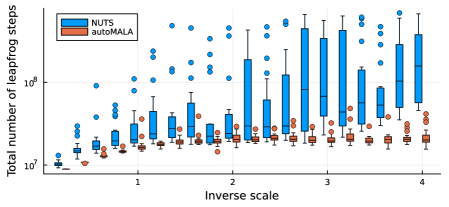
Figure 4: Total number of leapfrog steps used by autoMALA and NUTS for each scale parameter in Neal’s funnel.

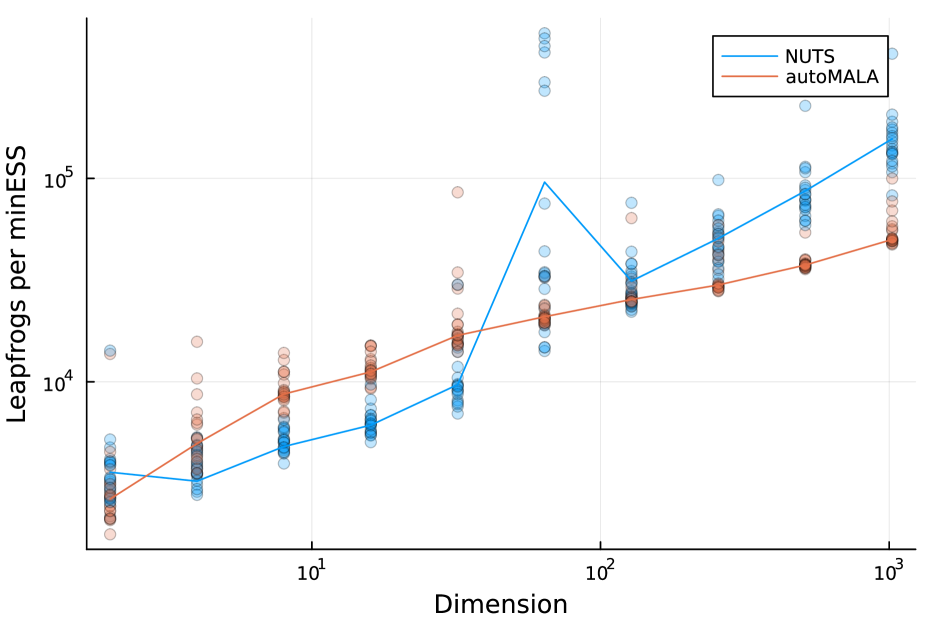
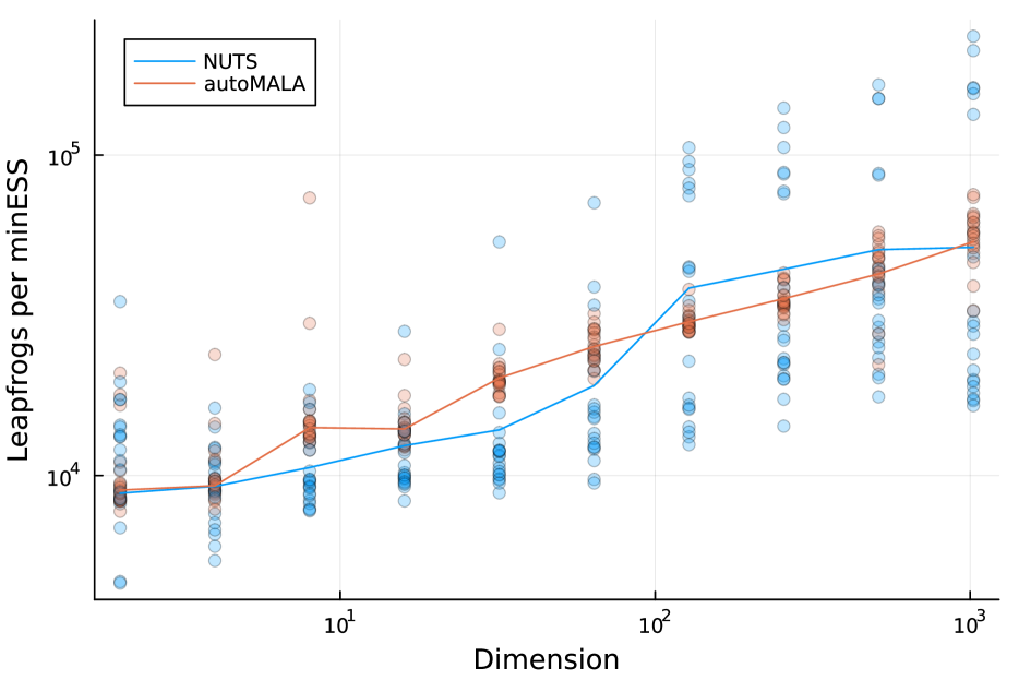
Figure 5: Number of leapfrog evaluations per 1000 minESS (lower is better) on targets with increasing dimension. Each point represents results from a separate seed for the experiment. Bold curves indicate averages across seeds. Left to right: Neal’s funnel, banana distribution, and multivariate normal distribution.

4.1 Varying local geometry

We first investigate the performance of autoMALA on targets with varying local geometry. There are two target distributions that we consider for this first synthetic example: Neal’s funnel and a banana distribution. Both targets contain a scale parameter that we can tune to make the distributions more difficult to sample from (greater variation in local geometry); difficulty increases as the scale parameter approaches zero. We compare autoMALA to NUTS: NUTS automatically adapts the number of leapfrog steps, but fixes a single step size after an initial warmup. In cases like the funnel, where the target distribution requires both very large and very small steps, the NUTS step size will be too large in the narrow part of the funnel; varying the number of leapfrog steps will not resolve the issue. Furthermore, note again that $n$ steps of doubling the trajectory length for NUTS takes compute time proportional to $2^{n}$, whereas $n$ steps of step size doubling in the autoMALA algorithm has a cost proportional to $n$. Therefore, for distributions with variable local geometries, we expect dynamic step size selection (autoMALA) to have a lower per-cost step compared to trajectory length selection (NUTS), and also less running time variability.

In Fig. 3 we see that autoMALA outperforms NUTS in terms of the number of leapfrog evaluations per minESS when applied to Neal’s funnel. We also see that autoMALA provides significantly more accurate estimates of the mean and variance on the first marginal (i.e., the “difficult” marginal direction along the elongated funnel). Moreover, autoMALA provides improved statistical performance despite using significantly fewer leapfrog steps, as shown in Fig. 4, as well as providing a smaller variability in the number of leapfrog steps. This makes autoMALA more suitable for distributed MCMC algorithms with synchronization, such as parallel tempering, where it is desirable for the runtime across machines to be approximately equal (Syed et al.,, 2021; Surjanovic et al.,, 2022, 2023). Similar results hold for the scaled banana distribution (see supplement), although there is less variation in geometry and so the two samplers are more comparable.

As a cautionary point, note that standard estimates of the ESS can be potentially misleading in these problems; the $\text{ESS}(\mu,\sigma)$ is more reliable. In particular, before reaching stationarity—which can take a long time for difficult problems—it is possible for the ESS estimate to be very high, even though the obtained samples do not resemble the target distribution. For instance, even though draws from NUTS are not representative of the target distribution, standard ESS estimates can still be very high (see the supplement). When target marginal means and variances are known, which is typical in synthetic problems, we recommend using the $\text{ESS}(\mu,\sigma)$ for evaluation, which can detect poor mixing via a misestimated mean and variance.

4.2 Dimensional scaling

Fig. 5 shows an investigation of the scaling properties of autoMALA as the dimension increases for the funnel, banana, and normal distributions. We again compare to NUTS, which is known for its favourable scaling properties on i.i.d. high-dimensional target distributions (Beskos et al.,, 2013), in terms of the number of leapfrog evaluations per effective sample. The results for the normal target agree with this theory, with NUTS performing better. In contrast, autoMALA is highly competitive in the two targets with extreme variation in local geometry, achieving the same efficiency values and scaling law as NUTS.

4.3 Step size convergence

Round-based autoMALA with a doubling of the number of MCMC iterations at each round (Algorithm 3) should converge to a reasonable choice of initial step size, $\epsilon_{\text{init}}$. Fig. 6 shows the chosen autoMALA default step size as a function of the tuning round for the three synthetic targets (banana, funnel, normal). In general, we see that the initial step size guess converges as the tuning rounds proceed. We note that generally a greater number of tuning rounds is needed for the step size to converge when autoMALA is applied to higher-dimensional distributions, due to a greater degree of Monte Carlo estimate variability, as explained in the supplement.

Figure 6: autoMALA initial step sizes as a function of the tuning round for $d=2$. Each new tuning round corresponds to a doubled number of samples used to estimate the initial step size. Results for higher-dimensional targets are provided in the supplement.

4.4 Comparison to non-adaptive algorithms

It is of interest to compare autoMALA to its non-adaptive predecessor MALA. To this end, we first perform a long run of autoMALA and retrieve its final step size $\epsilon_{\text{final}}$. We then do a grid search for a MALA step size targeting an acceptance probability of 0.574, a value known to be optimal for various types of targets (Roberts and Rosenthal,, 1998). Fig. 7 shows that $\epsilon_{\text{final}}$ is a good proxy for the optimal MALA step size with respect to the ideal Metropolis–Hastings acceptance probability.

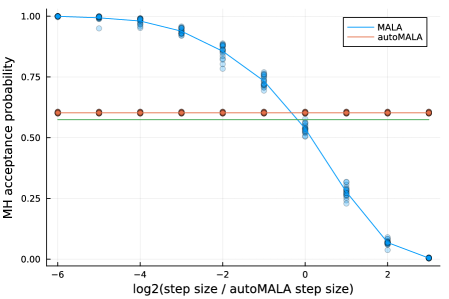
Figure 7: Metropolis–Hastings acceptance probability for autoMALA and MALA as a function of the initial step size for Neal’s funnel ($d=2$). The green horizontal line indicates the theoretical optimal 0.574 acceptance probability for MALA. Step sizes are selected relative to the optimal autoMALA step size.

We additionally assess the robustness (and lack thereof) of round-based autoMALA and MALA with respect to the initial step size. We find that even with very poor choices for the initial step size with autoMALA, we are able to converge to a reasonable step size that yields adequate acceptance probabilities. This is not the case for MALA, where the acceptance probabilities depend very heavily on the selected step size (see supplement).

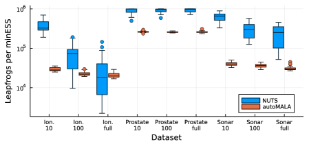
Figure 8: Number of leapfrog evaluations per 1000 minESS (lower is better) for the horseshoe variable selection model on three datasets with varying random subsampling.

4.5 Real data experiments

Finally, we compare autoMALA and NUTS on three joint variable selection and binary classification tasks: a dataset of radar returns from the ionosphere (Sigillito et al.,, 1989); data of sonar signals to distinguish metal from rock objects (Sejnowski and Gorman,, 1988), and the prostate cancer dataset from Piironen and Vehtari, (2018). For each dataset we use a Bayesian logistic regression model with a horseshoe prior to induce sparsity on the weights of the predictors (Carvalho et al.,, 2009). When the number of observations is low, the horseshoe prior creates varying geometries: the inclusion probabilities are non-degenerate, so as the sampler runs, the number of “active” variables—i.e., the effective dimensionality—changes, and so does the appropriate step size to use.

To investigate the small-data regime, we form two additional versions of each of the datasets by randomly sub-sampling $10$ and $100$ observations—for a total of $9$ possible combinations. We then run autoMALA and NUTS on all for $2^{14}$ iterations, and repeat this process $20$ times. Since there is no parameter in the model with known distribution, we compute minESS by taking the minimum over two different ESS estimators—batch means and auto-covariance estimation—across all parameters. Fig. 8 reports the results of this experiment, showing that autoMALA generally outperforms NUTS. As anticipated, the difference in performance is higher in the low data regime due to varying geometries in the target distributions.

5 CONCLUSION

This work introduced a new MCMC method, autoMALA, that can be thought of as the Metropolis-adjusted Langevin algorithm with a step size that is automatically selected at each iteration to adapt to local target distribution geometry. We proved that autoMALA preserves the correct stationary distribution despite its adaptivity. Further, we developed a round-based tuning procedure that automatically finds a reasonable initial step size guess and leapfrog step preconditioner matrix. In our experiments we observed that autoMALA performs well on various target distributions and outperforms NUTS when applied to target distributions with varying local geometry.

There are several directions for future research. As mentioned in Section 3, a proof of the irreducibility of autoMALA is left for future work. We posit that a two-step analysis of the Markov kernel—similar to the one carried out for NUTS in Durmus et al., (2023, Thm. 8)—should be enough to prove irreducibility. Additionally, it would be interesting to analyze if there are better choices than the uniform distribution over $\Delta$ for the pair $(a,b)$. Alternatively, a non-reversible update strategy for the pair $(a,b)$—as done in Neal, (2020) for the Metropolis acceptance decision—might introduce desirable persistence in the behavior of autoMALA. Finally, we note that the proposed automatic step size selection procedure can be generalized and extended to other involution-based samplers whose performance is critically dependent on one or a few hyperparameters.

Acknowledgements

ABC and TC acknowledge the support of an NSERC Discovery Grant. SS acknowledges the support of EPSRC grant EP/R034710/1 CoSines and NS acknowledges the support of a Vanier Canada Graduate Scholarship. We additionally acknowledge use of the ARC Sockeye computing platform from the University of British Columbia.

Checklist

1. For all models and algorithms presented, check if you include:

   1. A clear description of the mathematical setting, assumptions, algorithm, and/or model. [Yes/No/Not Applicable]

   2. An analysis of the properties and complexity (time, space, sample size) of any algorithm. [Yes/No/Not Applicable]

   3. (Optional) Anonymized source code, with specification of all dependencies, including external libraries. [Yes/No/Not Applicable]

2. For any theoretical claim, check if you include:

   1. Statements of the full set of assumptions of all theoretical results. [Yes/No/Not Applicable]

   2. Complete proofs of all theoretical results. [Yes/No/Not Applicable]

   3. Clear explanations of any assumptions. [Yes/No/Not Applicable]

3. For all figures and tables that present empirical results, check if you include:

   1. The code, data, and instructions needed to reproduce the main experimental results (either in the supplemental material or as a URL). [Yes/No/Not Applicable]

   2. All the training details (e.g., data splits, hyperparameters, how they were chosen). [Yes/No/Not Applicable]

   3. A clear definition of the specific measure or statistics and error bars (e.g., with respect to the random seed after running experiments multiple times). [Yes/No/Not Applicable]

   4. A description of the computing infrastructure used. (e.g., type of GPUs, internal cluster, or cloud provider). [Yes/No/Not Applicable]

4. If you are using existing assets (e.g., code, data, models) or curating/releasing new assets, check if you include:

   1. Citations of the creator if your work uses existing assets. [Yes/No/Not Applicable]

   2. The license information of the assets, if applicable. [Yes/No/Not Applicable]

   3. New assets either in the supplemental material or as a URL, if applicable. [Yes/No/Not Applicable]

   4. Information about consent from data providers/curators. [Yes/No/Not Applicable]

   5. Discussion of sensible content if applicable, e.g., personally identifiable information or offensive content. [Yes/No/Not Applicable]

5. If you used crowdsourcing or conducted research with human subjects, check if you include:

   1. The full text of instructions given to participants and screenshots. [Yes/No/Not Applicable]

   2. Descriptions of potential participant risks, with links to Institutional Review Board (IRB) approvals if applicable. [Yes/No/Not Applicable]

   3. The estimated hourly wage paid to participants and the total amount spent on participant compensation. [Yes/No/Not Applicable]

 

Supplementary Materials

 

Appendix A PROOFS

Proof of Theorem 3.3.

We split the proof into two cases depending on the value of $\delta$ in Line 6 of Algorithm 2: $\delta=-1$ and $\delta=1$. From this point on, fix any $s=(x,p,a,b)\in\mathcal{S}$ and $\epsilon_{\text{init}}>0$.

If $\delta=-1$, our initial step size was too large and we begin our step size halving procedure. Our claim is that there exists an $0<\epsilon^{\prime}<\epsilon_{\text{init}}$ such that if $s^{\prime}=(L_{\epsilon^{\prime}}(x,p),a,b)$, then $\ell(\epsilon^{\prime})=\log\bar{\pi}(s^{\prime})-\log\bar{\pi}(s)>\log(a)$. Once we show this, it follows that $\tau(s,\epsilon_{\text{init}})<\infty$ by our use of the step size halving procedure. To see that this claim holds, observe that by combining the leapfrog steps in Eq. 7, we have for any $\epsilon>0$ that

$$L_{\epsilon}(x,p)=(\tilde{x}(\epsilon),\tilde{p}(\epsilon)),$$ (16)

where

$$\tilde{x}(\epsilon) =x+\epsilon M^{-1}p+\frac{\epsilon^{2}}{2}M^{-1}\nabla\log\gamma(x)$$ (17)

$$\tilde{p}(\epsilon) =-\left(p+\frac{\epsilon}{2}\nabla\log\gamma(x)+\frac{\epsilon}{2}\nabla\log\gamma(\tilde{x}(\epsilon))\right).$$ (18)

From the continuous differentiability of $\pi$ (and hence $\log\gamma$), it follows that $\tilde{x}(\epsilon)\to x$ and $\tilde{p}(\epsilon)\to-p$ as $\epsilon\to 0$. This implies that $\ell(\epsilon)\to 0$ as $\epsilon\to 0$. We therefore require that $\log(a)<0$ to ensure that $\tau(s,\epsilon_{\text{init}})<\infty$.

If $\delta=1$, this means that the initial step size was too small and that we begin our step size doubling procedure. We claim that there exists an $\epsilon^{\prime}>\epsilon_{\text{init}}$ such that if $s^{\prime}=(L_{\epsilon^{\prime}}(x,p),a,b)$, then $\ell(\epsilon^{\prime})=\log\bar{\pi}(s^{\prime})-\log\bar{\pi}(s)<\log(b)$. Provided that $\log(b)>-\infty$, it suffices to prove that as $\epsilon\to\infty$, we have $\log\bar{\pi}(\tilde{x}(\epsilon),\tilde{p}(\epsilon),a,b)\to-\infty$. Using the expansion of the leapfrog step given by Eq. 17, observe that $\lvert\tilde{x}(\epsilon)\rvert\to\infty$ as $\epsilon\to\infty$, provided that either $p\neq 0$ or $\nabla\log\gamma(x)\neq 0$. Then, $\pi(\tilde{x}(\epsilon))\to 0$ as $\epsilon\to\infty$, by the assumption that $\pi(x)\to 0$ as $\lvert x\rvert\to\infty$. We conclude that $\bar{\pi}(\tilde{s})\to 0$ as $\epsilon\to\infty$, as well, because $0\leq\bar{\pi}(\tilde{s})\leq C\cdot\pi(\tilde{x})$ for some $C>0$.

Combining these two cases, we have that $\tau(s,\epsilon_{\text{init}})<\infty$ provided that $s$ satisfies the following conditions: $\log(a)<0$, $\log(b)>-\infty$, and $p\neq 0$. These conditions hold with probability one under $\bar{\pi}$, thereby completing the proof. ∎

Proof of Theorem 3.4.

We use Tierney, (1998, Theorem 2), more specifically, Corollary 2 (“deterministic proposal”). From Tierney, (1998, Theorem 2), standard calculations (reviewed, e.g., in Geyer, (2003)), establish that sufficient conditions for invariance of $K_{\mathrm{AM}}$ are: (1) that $Q_{\mathrm{AM}}$ is an involution, i.e., $Q_{\mathrm{AM}}=Q_{\mathrm{AM}}^{-1}$, and (2) that the set of points $s$ where the change of variable formula (Folland,, 1999, Thm. 2.47) applies has $\bar{\pi}$ probability one, and at those points, the absolute determinant of the Jacobian of $Q_{\mathrm{AM}}$ is one. We establish (1) and (2) in Lemmas A.1 and A.2 respectively. ∎

Lemma A.1.

The mapping $Q_{\mathrm{AM}}$ is an involution, $Q_{\mathrm{AM}}=Q_{\mathrm{AM}}^{-1}$.

Proof.

We split the argument into two sub-cases, either $s\in A$ (introduced in the main text), or $s\notin A$. If $s\notin A$, $Q_{\mathrm{AM}}$ is equal to the identity, so the involution property holds. Suppose now $s\in A$. We first show that for $s\in A$, $T\circ T(s)=s$. We have $T\circ T(s)=L_{\epsilon\circ T(s)}(T(s))$ by the definition of $T$. Next, since $s\in A$, $L_{\epsilon\circ T(s)}(T(s))=L_{\epsilon(s)}(T(s))$, again by definition. Applying again the definition of $T$, $L_{\epsilon(s)}(T(s))=L_{\epsilon(s)}\circ L_{\epsilon(s)}(s)$. Now, using the fact that the leapfrog is time-reversible (Neal,, 2011, §2.3), a synonym for the involution property in this context, we have $L_{\epsilon(s)}\circ L_{\epsilon(s)}(s)=s$. Finally, if $s\in A$, then by the above argument, $\epsilon\circ T\circ T(s)=\epsilon(s)$. Since $s\in A$, then $\epsilon(s)=\epsilon\circ T(s)$, hence $T(s)\in A$. This allows us to complete the argument: for $s\in A$, $Q_{\mathrm{AM}}\circ Q_{\mathrm{AM}}(s)=Q_{\mathrm{AM}}\circ T(s)$, and using $T(s)\in A$, $Q_{\mathrm{AM}}\circ T(s)=T\circ T(s)=s$. ∎

Lemma A.2.

Under the conditions of Theorem 3.4, there exists an open set $G\subset\mathcal{S}$ such that:

1. $\bar{\pi}(G)=1$,

2. $Q_{\mathrm{AM}}$ is continuously differentiable on $G$ with $|\det\nabla Q_{\mathrm{AM}}|=1$.

Proof of Lemma A.2.

We start by identifying a “bad” set $B$ of potential discontinuities. We will then show it is $\bar{\pi}$-null, and finally, use its complement as a building block for the “good” set $G$ satisfying the differentiability conditions from point 2. of the above statement.

Construction of the bad set. For any given point $s=(z,a,b)\in\mathcal{S}$, where $z=(x,p)$, note that the set of states that one autoMALA step could visit is countable (by step, we mean one iteration of the for loop in Algorithm 1 of the main text; by visit, we mean evaluation of the density at a point, the creation of state for which such evaluations occur are at Lines 11–13 of Algorithm 1, which in turn call Algorithm 2, where evaluations occur at Line 13). Define the trace of autoMALA as the countable set

$$\mathcal{T}_{s}=\{\Phi_{0}(s),\Phi_{1}(s),\ldots\},$$ (19)

where $\Phi_{i}(z)$ is the $i^{\text{th}}$ point visited by autoMALA in Lines 11 or 13 of Algorithm 1. (Any ordering suffices for our purposes.) By inspection of the algorithm, each $\Phi_{i}(s)$ is of the form $\Phi_{i}(s)=(L_{\epsilon_{i}}(z),a,b)$ (forward pass) or $(L_{\epsilon_{i}}\circ L_{\epsilon^{\prime}_{i}}(z),a,b)$ (reversibility check) for some $\epsilon_{i},\epsilon^{\prime}_{i}>0$. Define the set where we have a finite number of such evaluations as $F=\{s:\lvert\mathcal{T}_{s}\rvert<\infty\}$. By Theorem 3.3, we have $\bar{\pi}(F)=1$. We also define a superset to the trace, the potential trace of autoMALA $\bar{\mathcal{T}}_{s}$:

$$\mathcal{T}_{z} =\{L_{\epsilon_{\text{init}}2^{i}}(z):i\in\mathbb{Z}\},$$ (20)

$$\bar{\mathcal{T}}_{s} =\mathcal{T}_{z}\cup\left(\bigcup_{\tilde{z}\in\mathcal{T}_{z}}\mathcal{T}_{\tilde{z}}\right)\times\{a\}\times\{b\},$$ (21)

constructed so that the mappings contained in $\bar{\mathcal{T}}_{s}$ depend only on $z$ (and not on $a,b$, in contrast to $\Phi_{i}(s)$), while also having $\mathcal{T}_{s}\subset\bar{\mathcal{T}}_{s}$. Since the potential trace $\bar{\mathcal{T}}_{s}$ is a countable union of countable sets, it is countable, so we index it as:

$$\bar{\mathcal{T}}_{s}=\{\bar{\Phi}_{0}(z),\bar{\Phi}_{1}(z),\ldots\}\times\{a\}\times\{b\}.$$ (22)

We now define a collection of bad points, $B$, that identify possible sources of discontinuity of $Q_{\mathrm{AM}}$:

$$B=\{s=(z,a,b):\ell_{ij}(s)\in\{\log a,\log b\},\text{for some}\,i\neq j,\,i,j\leq\lvert\mathcal{T}_{s}\rvert\},\qquad\ell_{ij}(s)=\log\bar{\pi}(\Phi_{i}(s))-\log\bar{\pi}(\Phi_{j}(s)).$$ (23)

Also, define

$$\bar{B} =\{s=(z,a,b):\bar{\ell}_{ij}(z)\in\{\log a,\log b\},\,i\neq j\},\qquad\bar{\ell}_{ij}(z)=\log\bar{\pi}(\bar{\Phi}_{i}(z))-\log\bar{\pi}(\bar{\Phi}_{j}(z)),$$ (24)

$$=\bigcup_{i\neq j}\{s:\bar{\ell}_{ij}(z)\in\{\log a,\log b\}\}$$ (25)

The bad set is null. Note that $B\subset\bar{B}$. We argue that $\bar{\pi}(B)=0$ by showing that $\bar{\pi}(\bar{B})=0$. To see this, note that by Tonelli’s theorem,

$$\bar{\pi}(\bar{B}) =2\int\pi(\mathrm{d}z)\int_{\Delta}\mathds{1}_{\bar{B}}(s)\,\mathrm{d}a\,\mathrm{d}b$$ (26)

$$\leq 2\int\pi(\mathrm{d}z)\sum_{i,j}\mathbb{P}(\bar{\ell}_{i,j}(z)\in\{\log A,\log B\}).$$ (27)

where $(A,B)\sim\text{Unif}(\Delta)$. Since $A,B$ are non-atomic random variables, i.e. for all $c\in[0,1]$, $\mathbb{P}(A=c)=\mathbb{P}(B=c)=0$, we have $\mathbb{P}(\bar{\ell}_{i,j}(z)\in\{\log A,\log B\})=0$ and hence $\bar{\pi}(\bar{B})=0$.

Construction of the good set. From here, set $G=F\cap B^{c}$. Note that from Theorem 3.3, $\bar{\pi}(F)=1$ and hence $\bar{\pi}(G)=1$.

Showing that the good set is open and satisfies 2. In the following, we use a re-parameterization $(u,v)=(\log a,\log b)$. For any $s=(x,p,u,v)\in G$ we would like to show that there exists a $\delta>0$ such that the differentiability statement 2. of the result hold in a ball of radius $\delta$, denoted $N_{\delta}(s)=\{\tilde{s}\in\mathcal{S}:\|s-\tilde{s}\|<\delta\}$. For $s\in G$ we have that $\min\{\lvert\ell_{ij}-u\rvert,\lvert\ell_{ij}-v\rvert\}>0$ for all $i,j\in\{1,2,\ldots,\lvert\mathcal{T}_{s}\rvert\}$ (otherwise if this minimum would be zero, we would have $s\in B$, contradicting $s\in G$ since $G=F\cap B^{c}$). Now, set

$$\delta_{\ell}=\min_{i,j\leq\lvert\mathcal{T}_{s}\rvert}\{\lvert\ell_{ij}-u\rvert,\lvert\ell_{ij}-v\rvert\}>0.$$ (28)

By the continuity of $\log\bar{\pi}\circ\Phi_{i}$ for all $i\in\{1,2,\ldots,\lvert\mathcal{T}_{s}\rvert\}$, we have that there exists a $\delta_{i}>0$ such that for all $\tilde{s}\in N_{\delta_{i}}(s)$ we have

$$\lvert\log\bar{\pi}(\Phi_{i}(\tilde{s}))-\log\bar{\pi}(\Phi_{i}(s))\rvert<\frac{\delta_{\ell}}{3}.$$ (29)

Then, taking $\delta=\min\{\delta_{1},\ldots,\delta_{\lvert\mathcal{T}_{s}\rvert},\delta_{\ell}/3\}$, we have that inside $N_{\delta}(s)$ all branching decisions made by the autoMALA algorithm are identical and hence for all $\tilde{s}\in N_{\delta}(s)$ we have that either $\{s,\tilde{s}\}\subset A$ or $\{s,\tilde{s}\}\subset A^{c}$. Also, $\epsilon(\tilde{s})=\epsilon(s)$ and hence $\epsilon$ is constant on $N_{\delta}(s)$.

Next, we verify that $Q_{\mathrm{AM}}(\tilde{s})$ is continuously differentiable in the ball $N_{\delta}(s)$. As noted above, $N_{\delta}(s)\subset A$ or $N_{\delta}(s)\subset A^{c}$, so we consider these two sub-cases in turn. If $\tilde{s}\in N_{\delta}(s)\subset A^{c}$, $Q_{\mathrm{AM}}(\tilde{s})=\tilde{s}$ for all $\tilde{s}$, which is differentiable and has $|\det\nabla Q_{\mathrm{AM}}(\tilde{s})|=1$. Otherwise, if $\tilde{s}\in N_{\delta}(s)\subset A$, we have $Q_{\mathrm{AM}}(\tilde{s})=L_{\epsilon(\tilde{s})}(\tilde{s})=L_{\epsilon(s)}(\tilde{s})$. Because the step size is constant in this neighbourhood, and by the differentiability of the leapfrog operator under the assumption that $\pi$ is twice continuously differentiable (Assumption 3.1), we have that $Q_{\mathrm{AM}}(\tilde{s})$ is also continuously differentiable in this case. Since $\epsilon(\cdot)|_{N_{\delta}(s)}\equiv\epsilon_{0}$ for some $\epsilon_{0}$, $Q_{\mathrm{AM}}|_{N_{\delta}(s)}=L_{\epsilon_{0}}(\cdot)|_{N_{\delta}(s)}$, and hence we obtain in this sub-case as well that $|\det\nabla Q_{\mathrm{AM}}(\tilde{s})|=1$, this time from standard properties of the leap-frog operator reviewed in the main text. ∎

Appendix B ADDITIONAL EXPERIMENTS

Below we offer additional details about our experiments and provide the full set of figures produced for each of the experiments. Unless otherwise stated, we counted the number of leapfrogs in the warmup and final phases, but only retained samples for computing the ESS and other statistics on the final phase.

B.1 Synthetic data and models

We lay out the synthetic data and models used in Section 4.

The $d$-dimensional Neal’s funnel with scale parameter $\beta>0$ and $d\geq 2$ is given by

$$X_{1}\sim\mathcal{N}(0,\,9),\qquad X_{2},\ldots,X_{d}\mid X_{1}=x_{1}\stackrel{{\scriptstyle iid}}{{\sim}}\mathcal{N}(0,\,\exp(x_{1}/\beta)).$$ (30)

Note that we write $\mathcal{N}(0,\sigma^{2})$ to denote a normal random variable with variance $\sigma^{2}$.

The $d$-dimensional banana distribution with scale parameter $\beta>0$ and $d\geq 2$ is given by

$$X_{1}\sim\mathcal{N}(0,\,10),\qquad X_{2},\ldots,X_{d}\mid X_{1}=x_{1}\stackrel{{\scriptstyle iid}}{{\sim}}\mathcal{N}(x_{1}^{2},\,\beta^{2}/10).$$ (31)

The $d$-dimensional normal distribution is in all cases given by

$$X_{1},\ldots,X_{d}\stackrel{{\scriptstyle iid}}{{\sim}}\mathcal{N}(0,\,1).$$ (32)

B.2 Varying local geometry

We carried out experiments comparing autoMALA to NUTS on Neal’s funnel and the banana distribution with varying scale parameters. As $\beta\to 0$, the sampling problem increases in difficulty. Figs. 9, 10 and 11 show various metrics used to assess autoMALA and NUTS for the two targets (a subset of the results for the funnel were already presented in Section 4). For the funnel distribution we considered values of the scale parameter $\beta\in\{1/0.2,1/0.4,1/0.6,\ldots,1/4.0\}$. For the banana distribution we used values of $\beta\in\{2^{13},2^{12},\ldots,2^{-6}\}$. We used 20 different seeds and $2^{20}$ samples for each seed to estimate statistics with $2^{20}$ samples to warm up and tune NUTS. We used the same number of samples for autoMALA in the banana case, but used only $19$ rounds for the funnel in order to match the overall computational effort of NUTS (see Fig. 4).

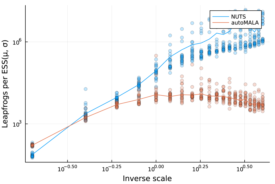
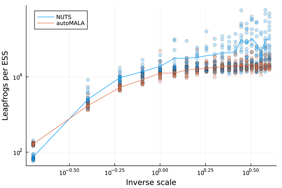
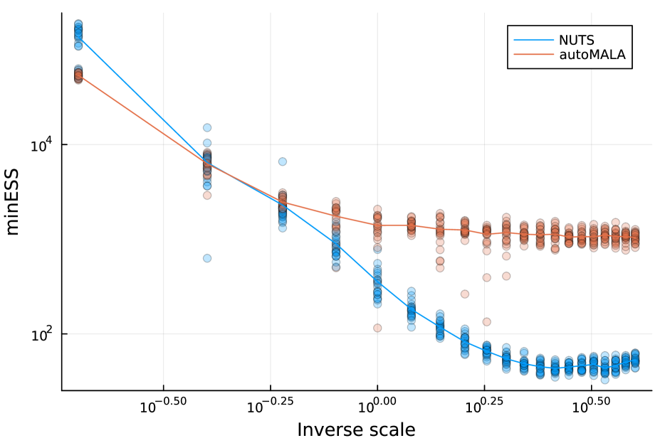
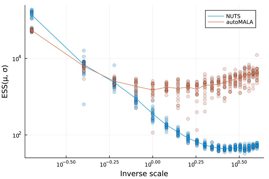
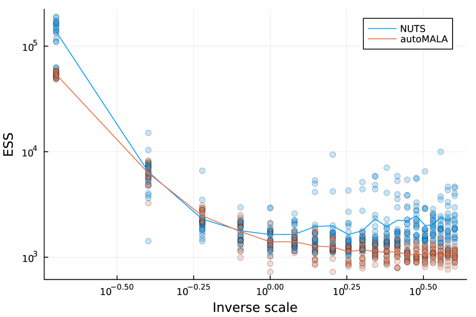
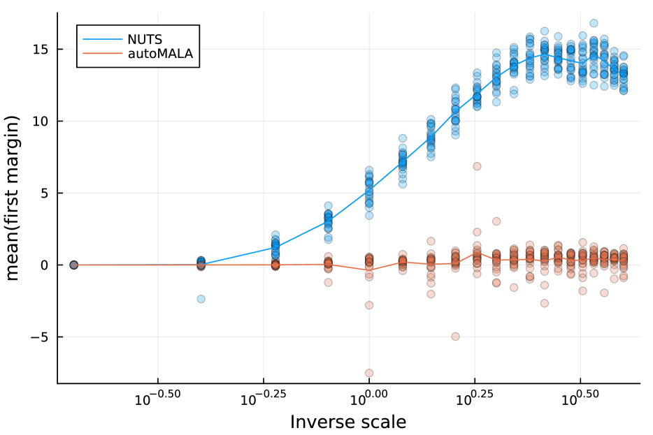
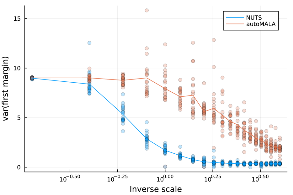
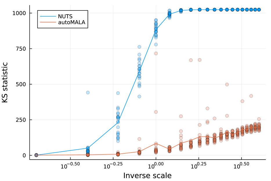
Figure 9: Various autoMALA and NUTS metrics for the scaled funnel experiments. Top row: Number of leapfrog steps per 1000 effective samples. From left to right we consider the minESS, $\text{ESS}(\mu,\sigma)$, and regular ESS. Middle row: minESS, $\text{ESS}(\mu,\sigma)$, and regular ESS. Bottom row: mean, variance, and Kolomogorov-Smirnov test statistic for the known first marginal of the distribution.

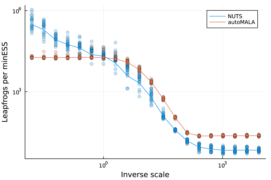
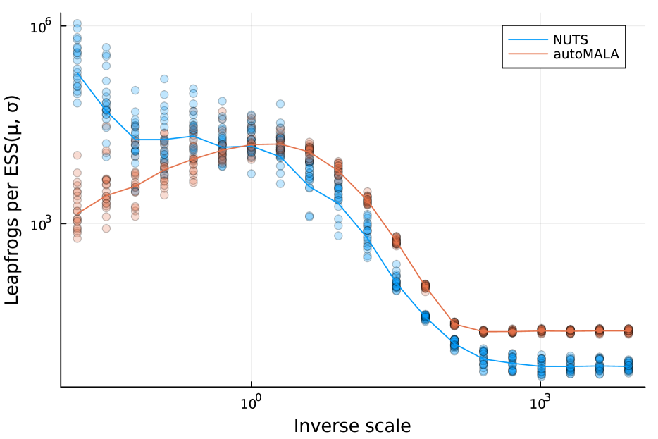
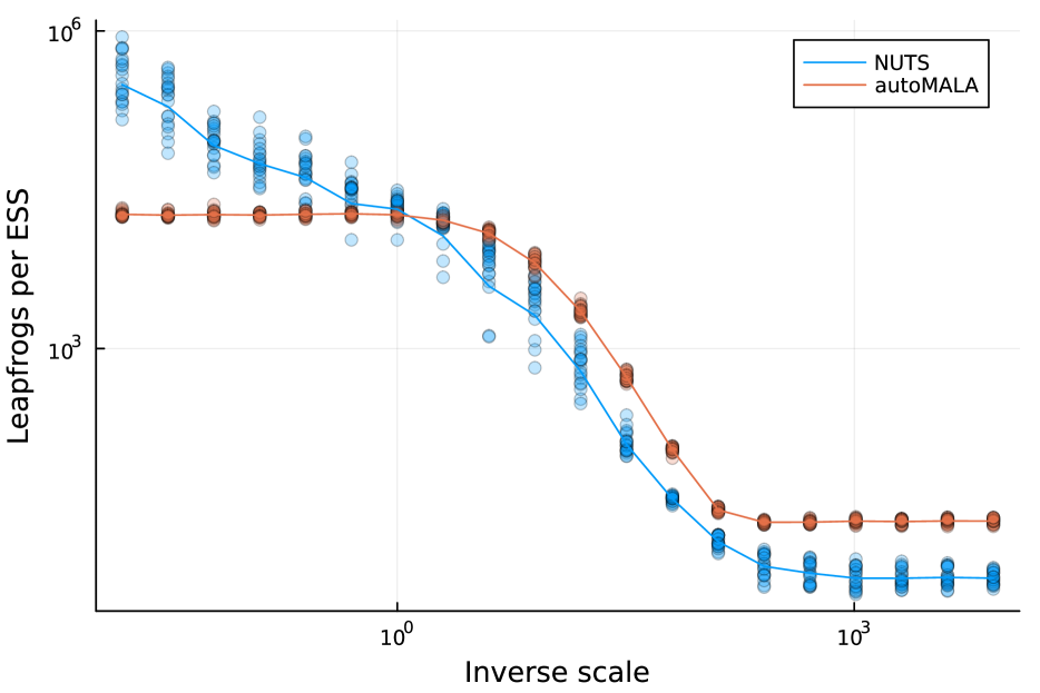
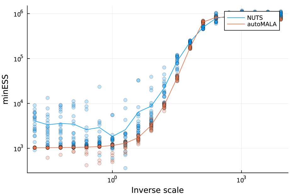
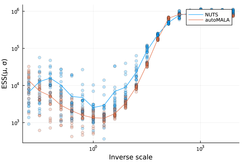
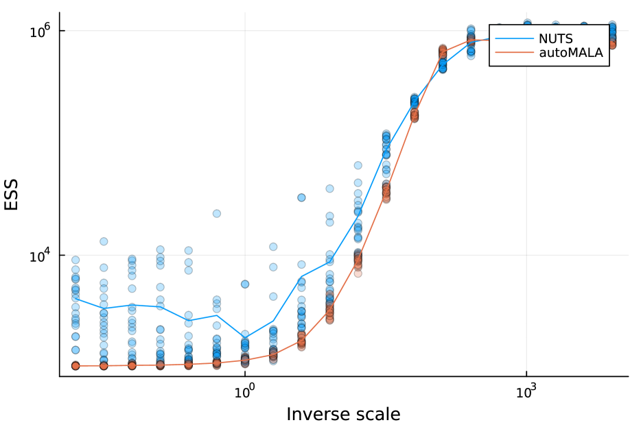
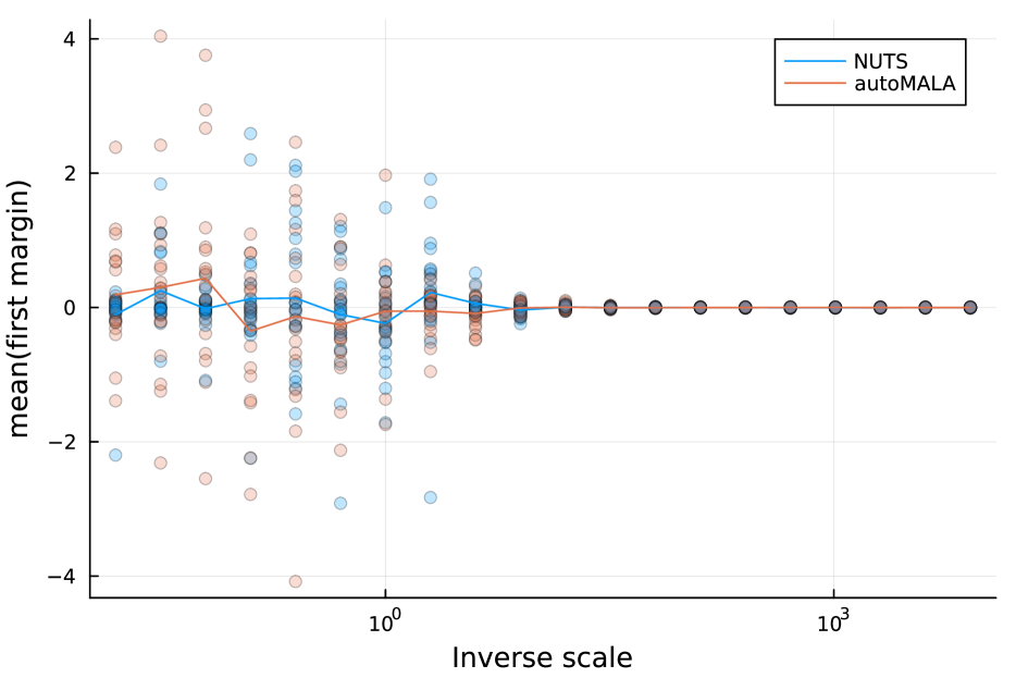
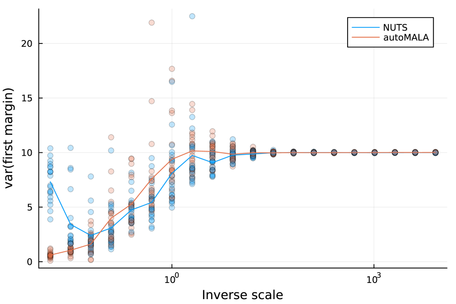
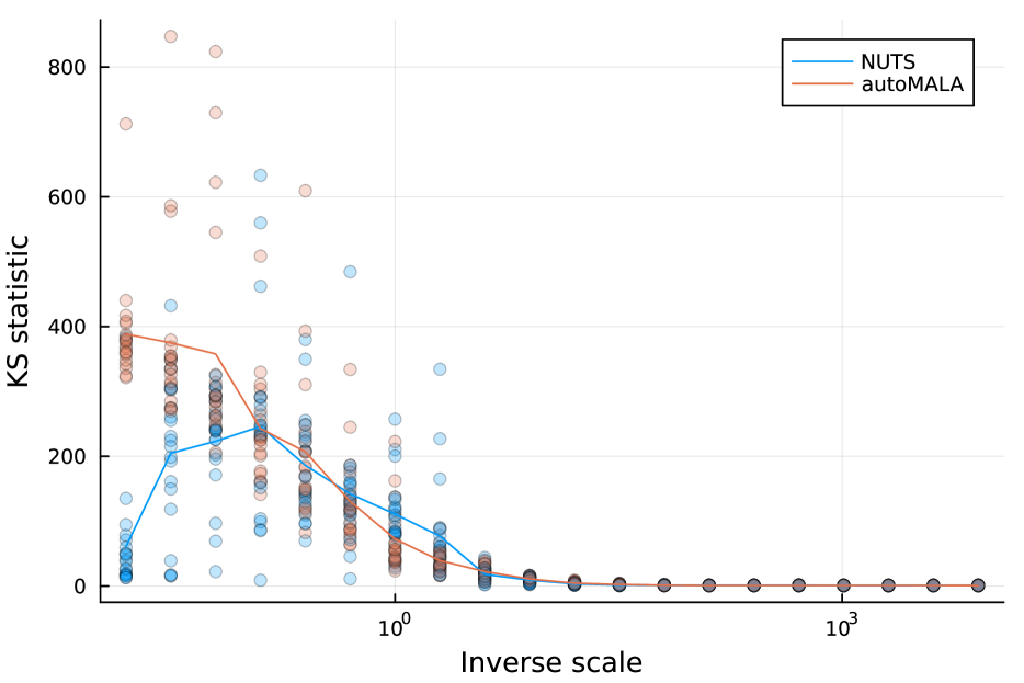
Figure 10: Various autoMALA and NUTS metrics for the scaled banana experiments. Top row: Number of leapfrog steps per 1000 effective samples. From left to right we consider the minESS, $\text{ESS}(\mu,\sigma)$, and regular ESS. Middle row: minESS, $\text{ESS}(\mu,\sigma)$, and regular ESS. Bottom row: mean, variance, and Kolomogorov-Smirnov test statistic for the known first marginal of the distribution.

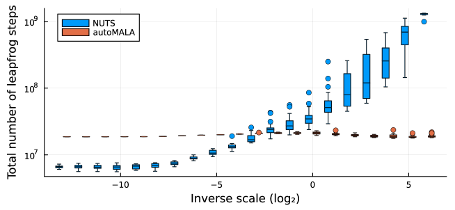
Figure 11: Number of leapfrog steps used by autoMALA and NUTS for each scale parameter of the banana distribution.

B.3 Dimensional scaling

The simulation results for the comparison of autoMALA to NUTS on various high-dimensional target distributions (funnel, banana, and normal) are presented in Fig. 12, Fig. 13, and Fig. 14. For all three distributions we used $d\in\{2^{1},2^{2},\ldots,2^{10}\}$ with 20 seeds and $2^{18}$ samples for each seed and $2^{18}$ samples for warmup for each seed. For Neal’s funnel we set $\beta=2$ and for the banana distribution we set $\beta=1$.

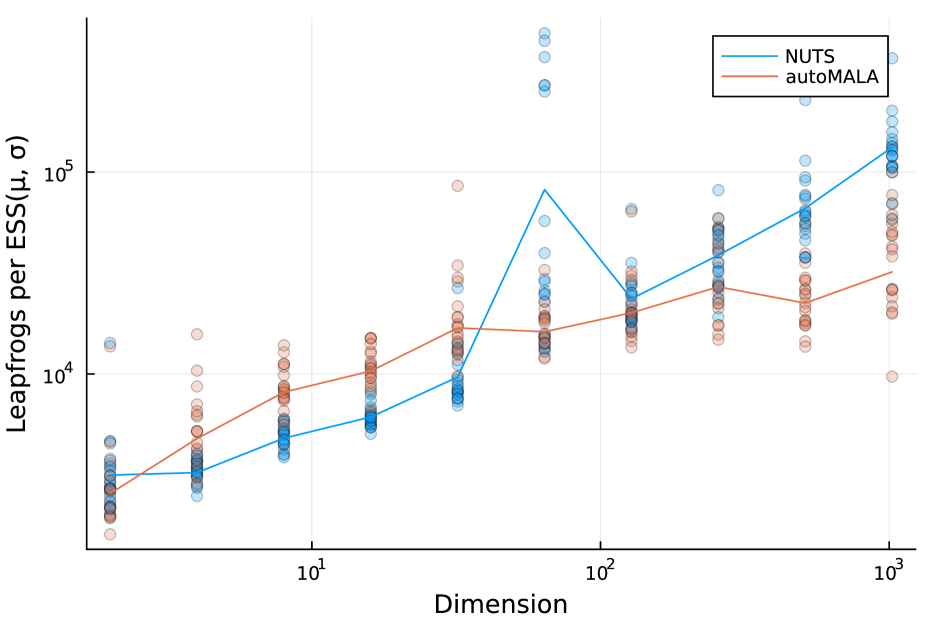
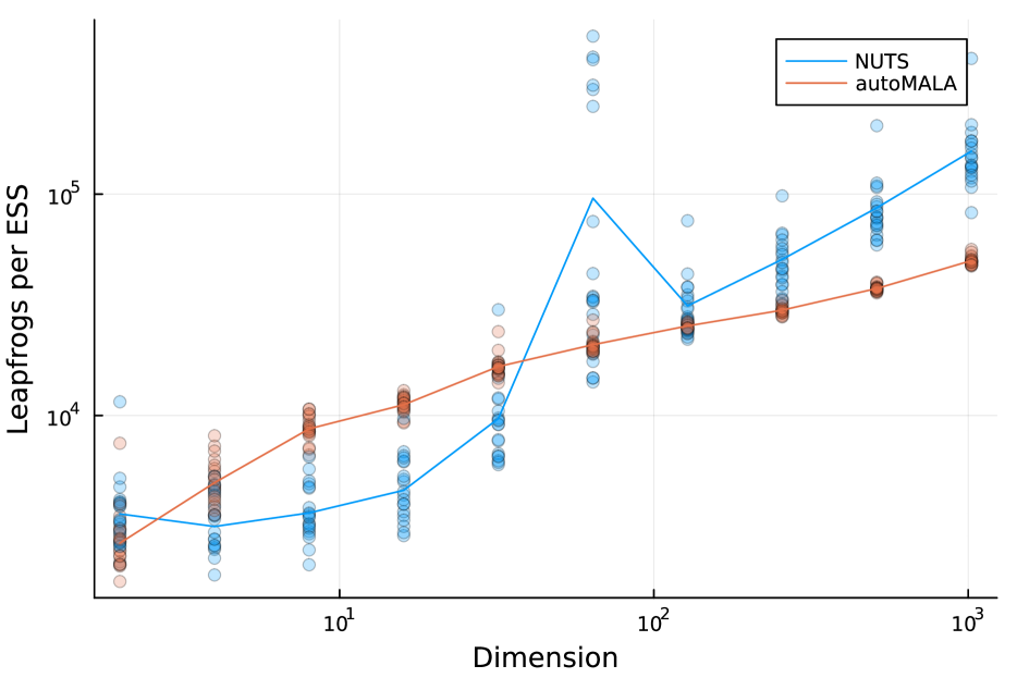
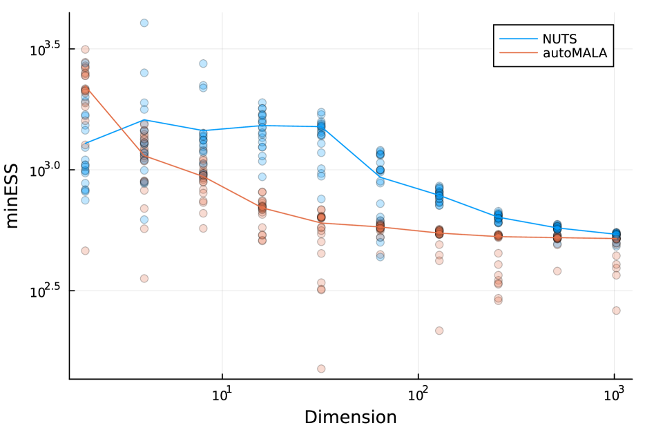
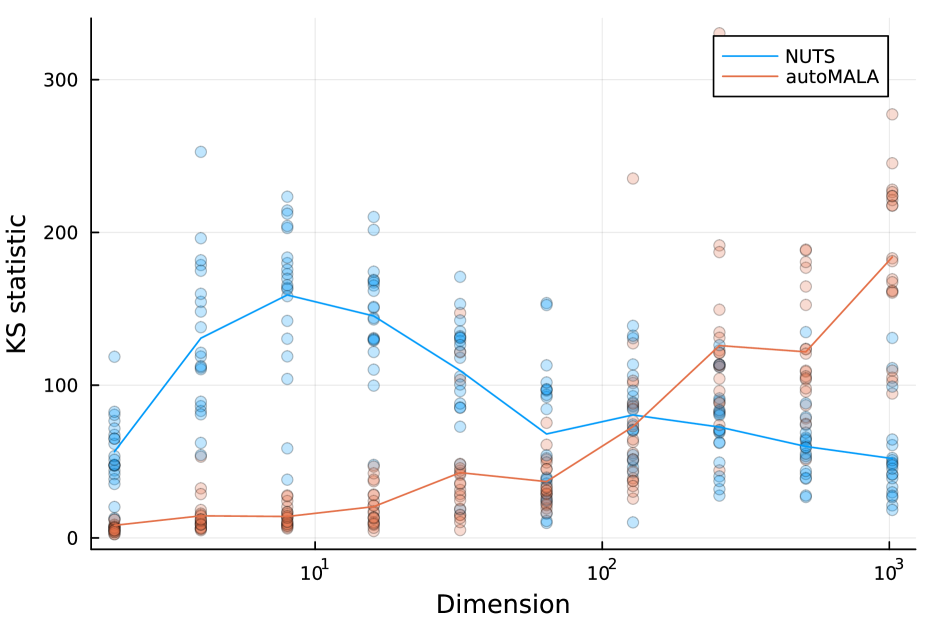
Figure 12: Various autoMALA and NUTS metrics for the high-dimensional funnel experiments. Top row: Number of leapfrog steps per 1000 effective samples. From left to right we consider the minESS, $\text{ESS}(\mu,\sigma)$, and regular ESS. Middle row: minESS, $\text{ESS}(\mu,\sigma)$, and regular ESS. Bottom row: mean, variance, and Kolomogorov-Smirnov test statistic for the known first marginal of the distribution.

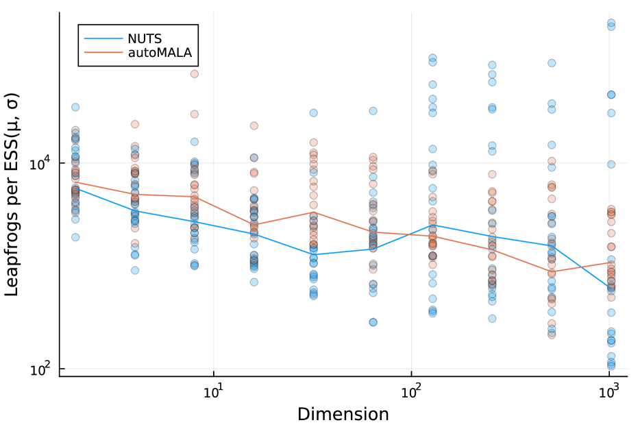
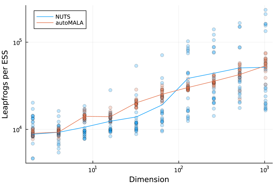
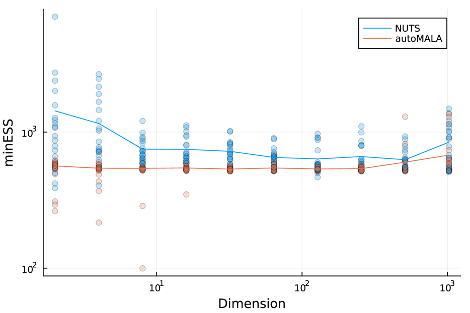
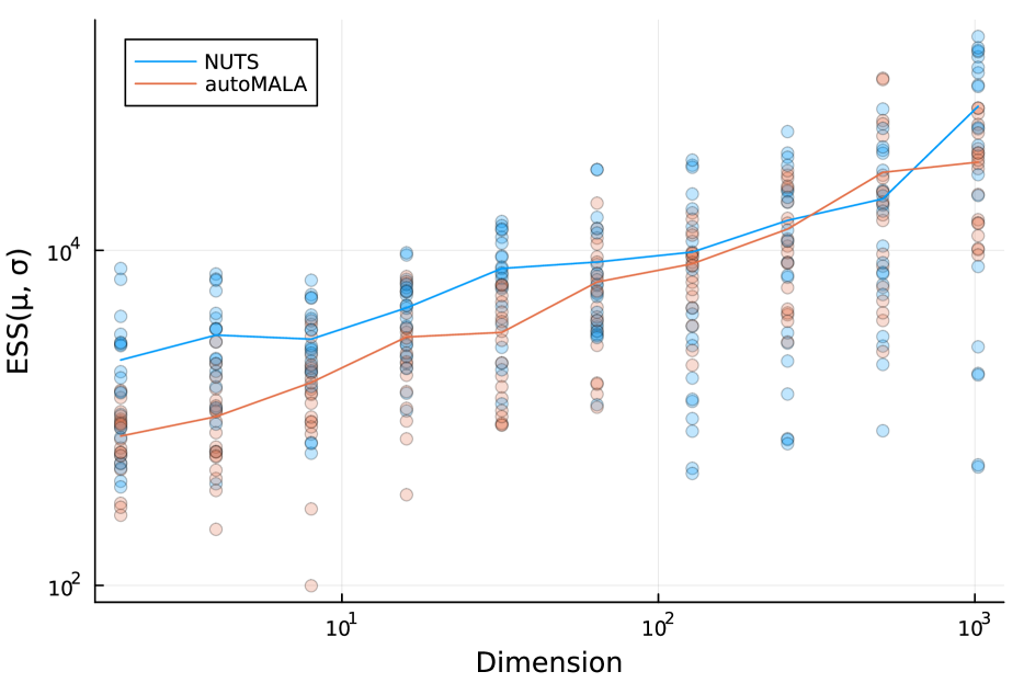
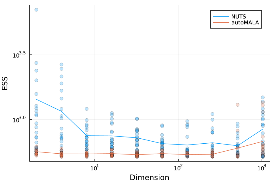
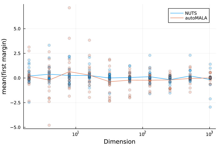
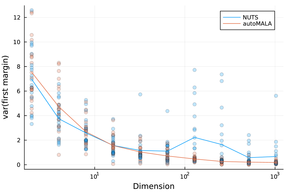
Figure 13: Various autoMALA and NUTS metrics for the high-dimensional banana experiments. Top row: Number of leapfrog steps per 1000 effective samples. From left to right we consider the minESS, $\text{ESS}(\mu,\sigma)$, and regular ESS. Middle row: minESS, $\text{ESS}(\mu,\sigma)$, and regular ESS. Bottom row: mean, variance, and Kolomogorov-Smirnov test statistic for the known first marginal of the distribution.

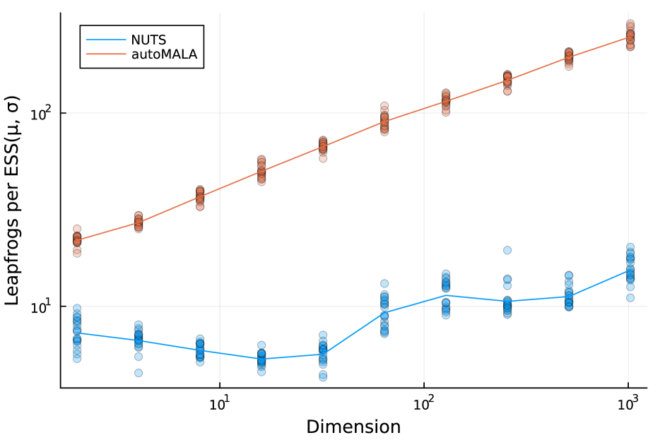
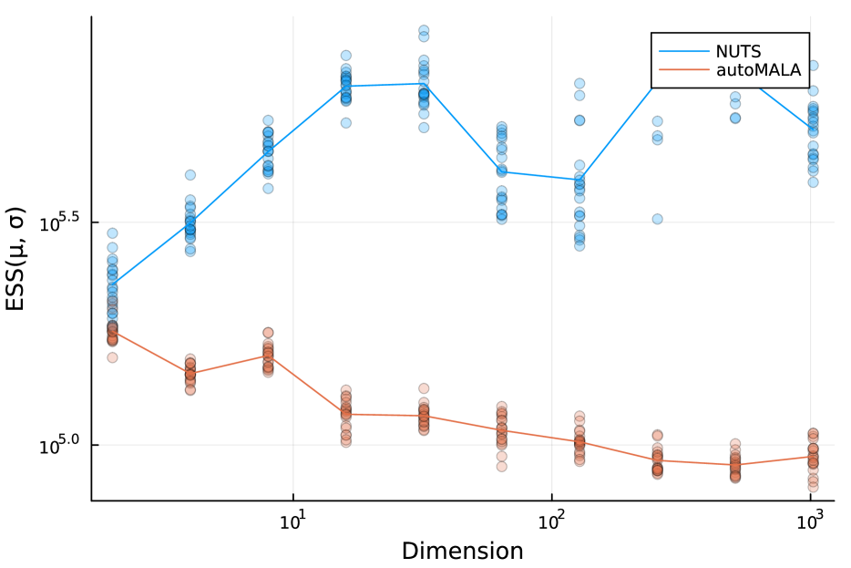
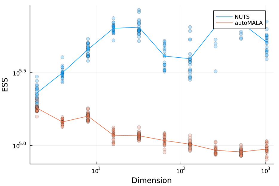
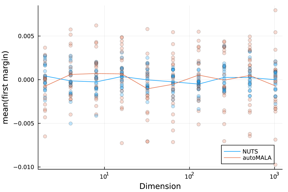
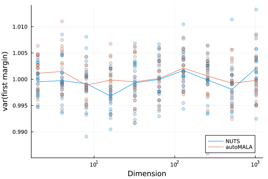
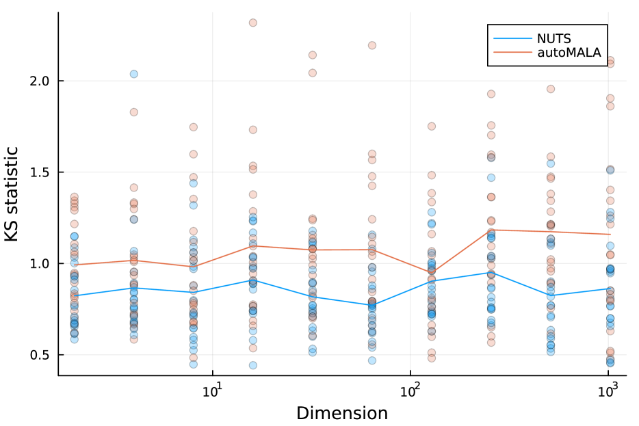
Figure 14: Various autoMALA and NUTS metrics for the high-dimensional normal experiments. Top row: Number of leapfrog steps per 1000 effective samples. From left to right we consider the minESS, $\text{ESS}(\mu,\sigma)$, and regular ESS. Middle row: minESS, $\text{ESS}(\mu,\sigma)$, and regular ESS. Bottom row: mean, variance, and Kolomogorov-Smirnov test statistic for the known first marginal of the distribution.

B.4 Step size convergence

We assessed whether the default step size, $\epsilon_{\text{init}}$, converges as the number of tuning rounds increases. Each successive tuning round used twice the amount of MCMC iterations compared to the previous tuning round. The experimental results for the three synthetic target distributions for various dimensions $d$ are presented in Fig. 15. In these experiments we used $d\in\{2^{1},2^{2},\ldots,2^{9}\}$, and 20 different seeds for each setting. For each combination of simulation settings, we ran autoMALA for $2^{19}$ iterations ($2^{18}$ samples for warmup and $2^{18}$ final samples).

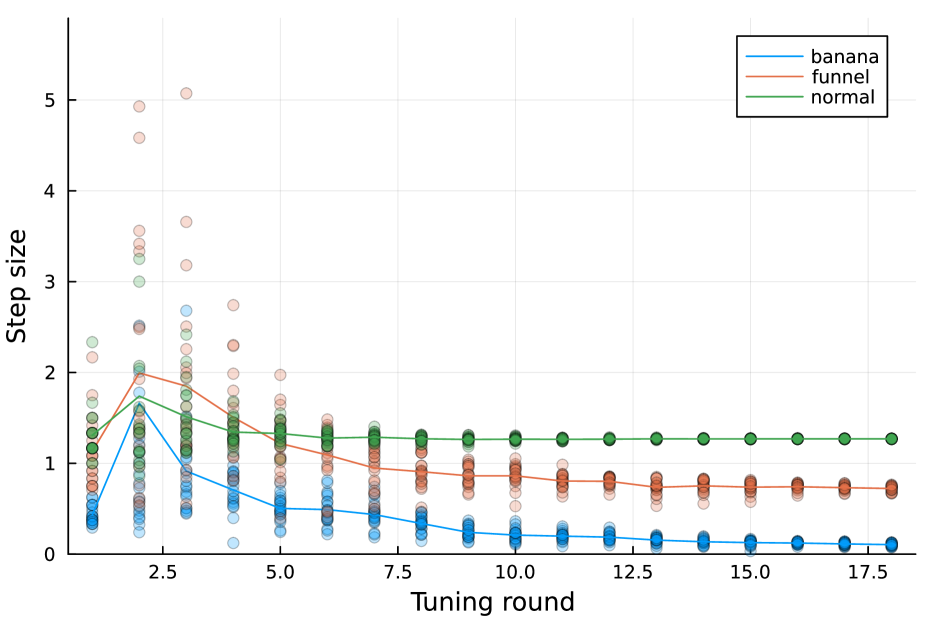
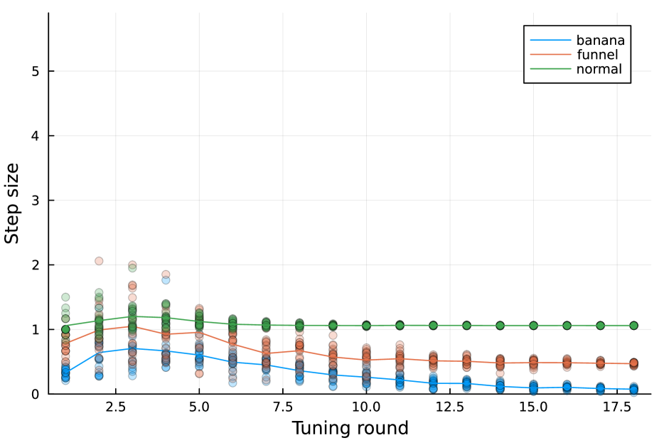
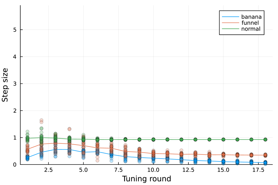
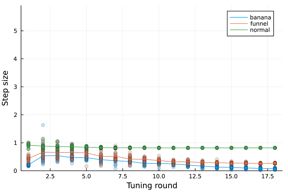
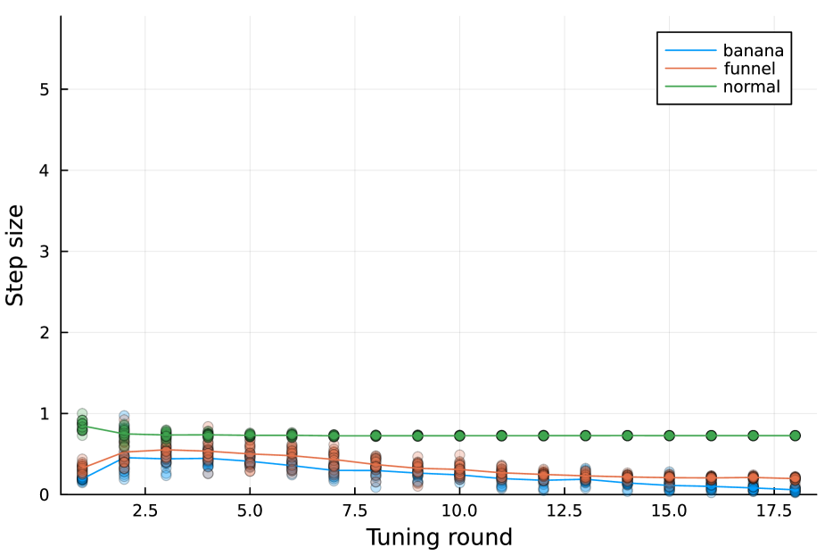
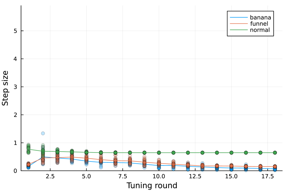
Figure 15: autoMALA default step sizes, $\epsilon_{\text{init}}$, as a function of the tuning round, where each tuning round doubles the number of samples used to estimate $\epsilon_{\text{init}}$. Top left to bottom right: $2^{j}$-dimensional target distributions for $j=1,2,\ldots,9$.

B.5 Comparison to non-adaptive algorithms

We compared autoMALA to MALA by considering both a fixed grid of step sizes and a grid relative to the “optimal” choice selected after a long run of autoMALA. Our main statistic is the average Metropolis–Hastings acceptance probability. For the fixed step size grid, we used 20 seeds for each of the three synthetic models with $d=2$. The final acceptance probabilities were calculated after running both autoMALA and MALA for $2^{18}$ warmup iterations followed by $2^{18}$ MCMC samples. We considered $\epsilon\in\{2^{-10},2^{-9},\ldots,2^{1}\}$. These results are presented in Fig. 16.

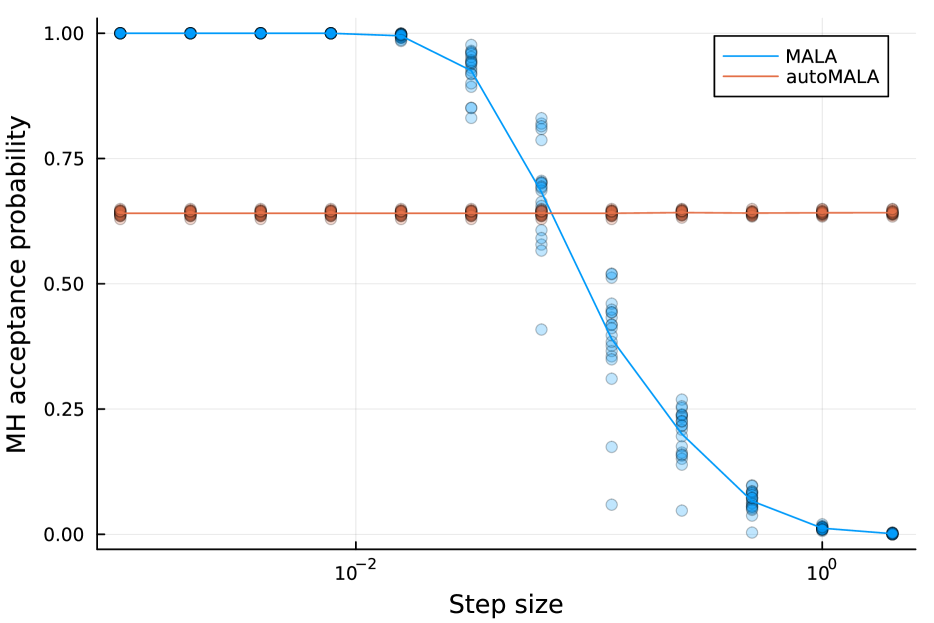
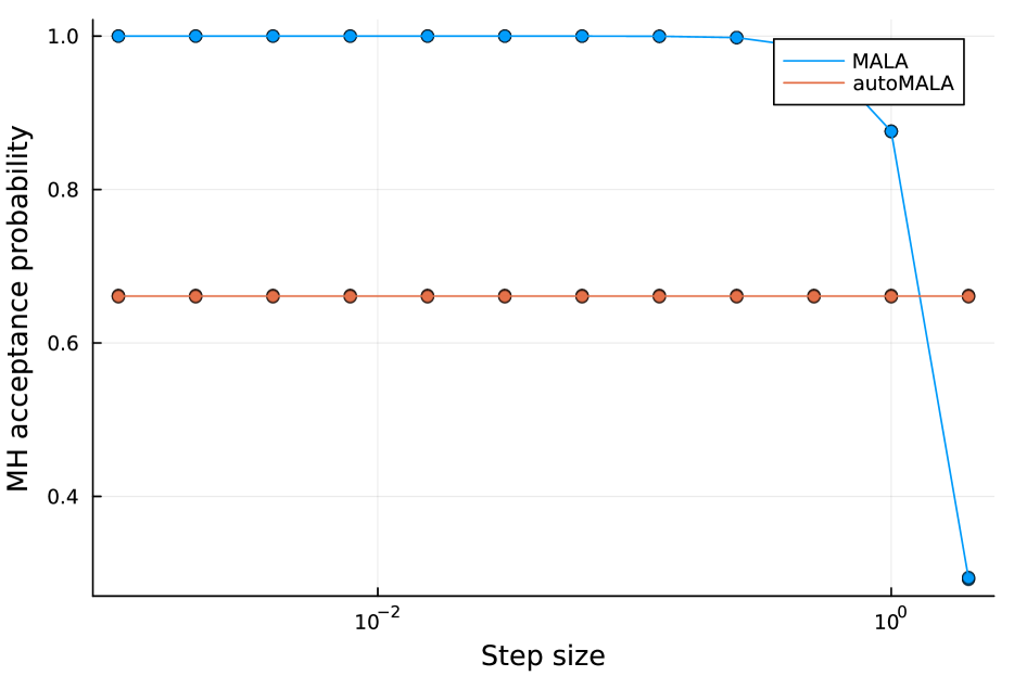
Figure 16: autoMALA and MALA acceptance probabilities as a function of initial step size for a fixed grid. Left to right: funnel, banana, and normal distributions ($d=2$).

For the step size grid relative to the “optimal” autoMALA choice, we also used 20 seeds applied to the three synthetic models. After running autoMALA for $2^{18}$ warmup iterations and $2^{18}$ final samples, we extracted the selected default step size (denoted $\epsilon$ here). Then, we ran MALA with step sizes in the range $\{\epsilon\cdot 2^{-6},\epsilon\cdot 2^{-5},\ldots,\epsilon\cdot 2^{3}\}$. We ran MALA for the same number of warmup and final samples as autoMALA. These results are presented in Fig. 17.

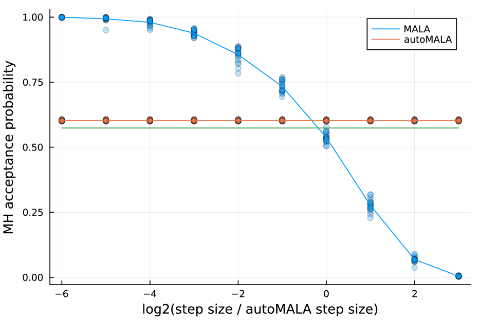
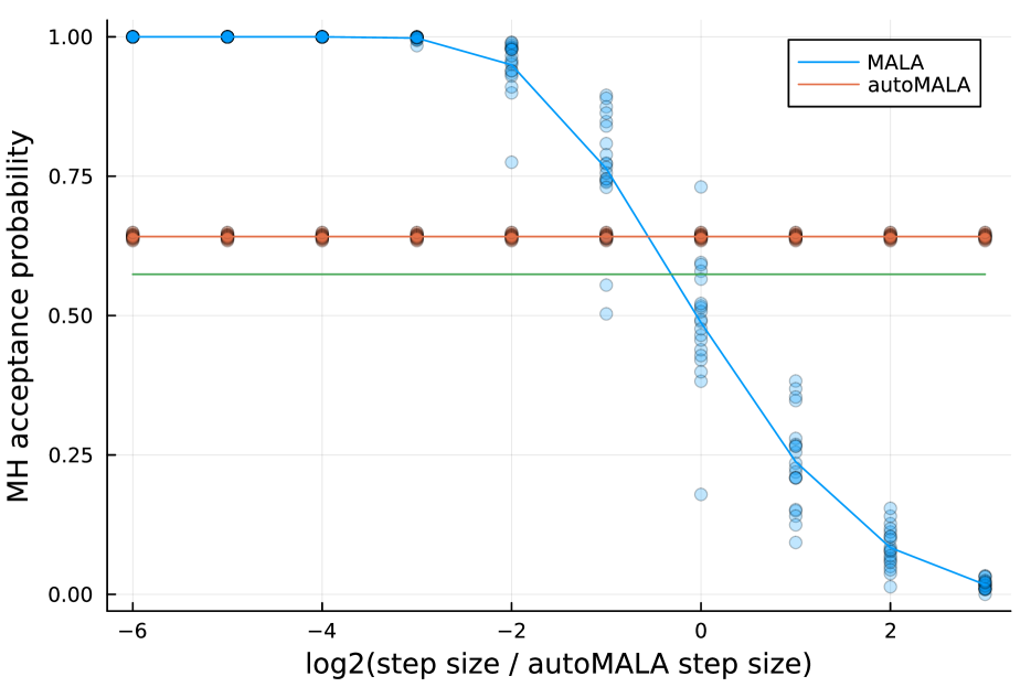
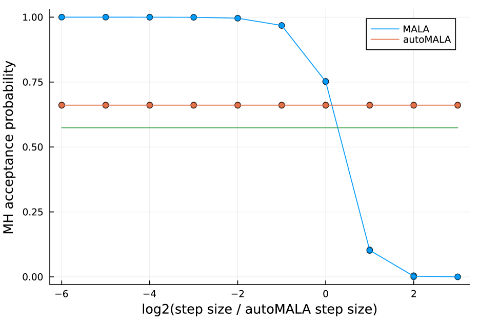
Figure 17: autoMALA and MALA acceptance probabilities as a function of initial step size for a grid relative to the optimal choice for autoMALA. Left to right: funnel, banana, and normal distributions ($d=2$).

B.6 autoMALA Metropolis–Hastings acceptance probability

The optimal acceptance probability for MALA on a certain class of target distributions as the dimension tends to infinity has been shown to be 0.574. autoMALA is a different algorithm than MALA, and hence its “optimal” acceptance probability might be different. We assess the MH acceptance probability of autoMALA on standard multivariate normal targets as the dimension tends to infinity. The results of these simulations are shown in Fig. 18. We see that the asymptotic autoMALA acceptance probability on the product distribution is close to the optimal MALA acceptance probability, but not exactly equal. In this experiment we used 20 different seeds with $2^{15}$ samples in the final round to estimate the step size. The simulations were run on distributions of dimension $d\in\{2^{1},2^{2},\ldots,2^{14}\}$.

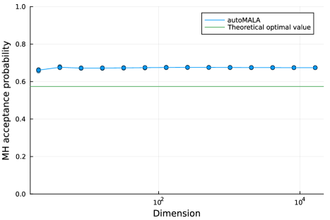
Figure 18: Metropolis–Hastings acceptance probability of autoMALA as a function of the dimension of a multivariate standard normal target distribution for various simulation seeds. The green line indicates the theoretical optimal MALA acceptance probability. Note that there is no guarantee that autoMALA should converge to the MALA acceptance probability because the algorithm is inherently different from MALA.

B.7 Fixed point of autoMALA step size objective

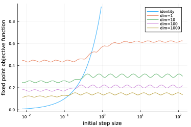
Figure 19: The objective function $g(\epsilon_{\text{init}})=\mathbb{E}_{\bar{\pi},\epsilon_{\text{init}}}[(\epsilon(S,\epsilon_{\text{init}})+\epsilon(S^{\prime},\epsilon_{\text{init}}))/2]$ for isotropic normal targets of varying dimension. The x-axis shows a grid over $\epsilon_{\text{init}}$ in log scale. The y-axis shows the function $g$ approximated using $2^{15}$ samples. The round-based scheme approaches the fixed point $\epsilon_{\text{init}}=g(\epsilon_{\text{init}})$. The identity function is shown (sharply increasing function, due to the x-axis being in log-scale).

We show in Fig. 19 the objective function $g(\epsilon_{\text{init}})=\mathbb{E}_{\bar{\pi},\epsilon_{\text{init}}}[(\epsilon(S,\epsilon_{\text{init}})+\epsilon(S^{\prime},\epsilon_{\text{init}}))/2]$ as a function of $\epsilon_{\text{init}}$, approximated using $2^{15}$ iterations of autoMALA for each grid point $\epsilon_{\text{init}}=2^{j}$ for $j\in\{-7,-6.9,-6.8,\dots,6.9,7\}$. This was repeated for isotropic normal targets of dimension $d\in\{1,10,100,1000\}$. In all cases, a unique fixed point is present upon inspection. Moreover, the shape of the objective appears to approximately converge to a constant function as $d$ increases, which suggests that the greater number of rounds required to converge in high dimensions is not necessarily due to the complexity of the idealized fixed point equation $\epsilon_{\text{init}}=g(\epsilon_{\text{init}})$, but rather due to the increased difficulty in approximating $g$ from Monte Carlo samples.

B.8 Preconditioning strategy

In Section 3 we described a simple strategy to obtain a robust diagonal preconditioner by taking a random mixture of the form

$$(\hat{\Sigma}_{\text{AM}})_{i,i}^{-1/2}=\eta\hat{\Sigma}_{i,i}^{-1/2}+(1-\eta),$$ (33)

with $\eta\sim{\mathrm{Beta}}(\tilde{\alpha},\tilde{\beta})$ sampled independently for some values of $\tilde{\alpha},\tilde{\beta}>0$. The justification of this strategy is that it adds robustness to the sampler when 1) the estimated standard deviations are far from their true values under the target distribution, or 2) the local geometry varies considerably so that a fixed preconditioner can fail in particulars regions of the space. On the other hand, the approach can cause issues when there are dimensions that have scales considerably smaller than $1$. Indeed, consider the bivariate distribution $\mathcal{N}(0,\operatorname{diag}(10^{-8},10^{8})^{2})$. When $\eta\sim{\mathrm{Unif}}(0,1)$,

$$\mathbb{E}[(\hat{\Sigma}_{\text{AM}})_{2,2}^{-1/2}|\hat{\Sigma}]=0.5\hat{\Sigma}_{2,2}^{-1/2}+0.5\approx 0.5\cdot 10^{-8}+0.5\approx 0.5.$$ (34)

Since $p\sim\mathcal{N}(0,\hat{\Sigma}_{\text{AM}}^{-1})$ (see Algorithm 1), this means that $p_{2}$ will on average be eight orders of magnitude larger than its optimal value (see e.g. Neal,, 2011, §4.1). In turn, this forces autoMALA to heavily shrink the step size at each iteration in order to reach the right scale, which results in slow performance.

Figure 20: Comparison of three versions of autoMALA alongside NUTS on two synthetic targets ($d=2$). Boxplots denote repetition for $20$ seeds. Lines mark the mean across repetitions. Left column: anisotropic normal (inverse scale corresponds to exponent $c$). Right column: funnel. Top to bottom: known margin mean, known margin variance, and leapfrog per minESS.

A slightly more complicated approach draws $\eta$ from a zero-one-inflated Beta distribution, which is a mixture between a Bernoulli and a Beta distribution

$${\mathrm{Beta}}_{01}(\mathrm{d}\eta;\tilde{\alpha},\tilde{\beta},p,m)=m{\mathrm{Bern}}(\mathrm{d}\eta;p)+(1-m){\mathrm{Beta}}(\mathrm{d}\eta;\tilde{\alpha},\tilde{\beta}),$$ (35)

for some $m,p\in[0,1]$. This approach has the benefit of letting the sampler use the exact adapted diagonal covariance matrix in some iterations. To investigate the benefits of this change, we ran NUTS alongside the following three versions of autoMALA:

1. Single preconditioner: $\eta\sim{\mathrm{Beta}}_{01}(1,1,1,1)$, so that $\operatorname{diag}(\hat{\Sigma}_{\text{AM}})=\operatorname{diag}(\hat{\Sigma})$.

2. Smooth preconditioner: $\eta\sim{\mathrm{Beta}}_{01}(1,1,1,0)$. This is the strategy described in Section 3.

3. Mixture preconditioner: $\eta\sim{\mathrm{Beta}}_{01}(1,1,1/2,2/3)$, so that the two endpoints $\{0,1\}$ and the interval $(0,1)$ have all equal chance ($1/3$) of being picked.

We ran these $4$ samplers on the funnel scale experiment already presented, and also on a simple $2$-dimensional anisotropic Gaussian parametrized so that the standard deviations are $(10^{-c},10^{c})$ for $c\in\mathbb{N}$. In this example we expect the single preconditioner approach to dominate, while the smooth approach should fail. This is exactly what is shown in Section B.8. Moreover, the mixture preconditioner is the second best performing after the single preconditioner. In contrast, the mixture approach dominates in the funnel target, although all three versions of autoMALA are considerably more efficient than NUTS.

References

- Atchadé, (2006) Atchadé, Y. F. (2006). An adaptive version for the Metropolis adjusted Langevin algorithm with a truncated drift. Methodology and Computing in applied Probability, 8:235–254.
- Atchadé and Rosenthal, (2005) Atchadé, Y. F. and Rosenthal, J. S. (2005). On adaptive Markov chain Monte Carlo algorithms. Bernoulli, 11(5):815 – 828.
- Beskos et al., (2013) Beskos, A., Pillai, N., Roberts, G., Sanz-Serna, J.-M., and Stuart, A. (2013). Optimal tuning of the hybrid Monte Carlo algorithm. Bernoulli, 19(5A):1501 – 1534.
- Carvalho et al., (2009) Carvalho, C. M., Polson, N. G., and Scott, J. G. (2009). Handling sparsity via the horseshoe. In International Conference on Artificial Intelligence and Statistics, volume 5, pages 73–80.
- Coullon et al., (2023) Coullon, J., South, L., and Nemeth, C. (2023). Efficient and generalizable tuning strategies for stochastic gradient MCMC. Statistics and Computing, 33(3):66.
- Durmus et al., (2023) Durmus, A., Gruffaz, S., Kailas, M., Saksman, E., and Vihola, M. (2023). On the convergence of dynamic implementations of Hamiltonian Monte Carlo and No U-Turn Samplers. arXiv e-prints, page arXiv:2307.03460.
- Flegal et al., (2008) Flegal, J. M., Haran, M., and Jones, G. L. (2008). Markov chain Monte Carlo: Can we trust the third significant figure? Statistical Science, 23(2):250–260.
- Folland, (1999) Folland, G. B. (1999). Real Analysis: Modern Techniques and Their Applications. Wiley, New York, second edition.
- Geyer, (2003) Geyer, C. (2003). The Metropolis–Hastings–Green Algorithm. Technical report, University of Minnesota, Department of Statistics.
- Girolami and Calderhead, (2011) Girolami, M. and Calderhead, B. (2011). Riemann manifold Langevin and Hamiltonian Monte Carlo methods. Journal of the Royal Statistical Society Series B: Statistical Methodology, 73(2):123–214.
- Hird and Livingstone, (2023) Hird, M. and Livingstone, S. (2023). Quantifying the effectiveness of linear preconditioning in Markov chain Monte Carlo. arXiv:2312.04898.
- Hoffman et al., (2014) Hoffman, M. D., Gelman, A., et al. (2014). The No-U-Turn Sampler: Adaptively setting path lengths in Hamiltonian Monte Carlo. Journal of Machine Learning Research, 15(1):1593–1623.
- Kleppe, (2016) Kleppe, T. S. (2016). Adaptive step size selection for Hessian-based manifold Langevin samplers. Scandinavian Journal of Statistics, 43(3):788–805.
- Kleppe, (2022) Kleppe, T. S. (2022). Connecting the dots: Numerical randomized Hamiltonian Monte Carlo with state-dependent event rates. Journal of Computational and Graphical Statistics, 31(4):1238–1253.
- Livingstone and Zanella, (2022) Livingstone, S. and Zanella, G. (2022). The Barker proposal: Combining robustness and efficiency in gradient-based MCMC. Journal of the Royal Statistical Society Series B: Statistical Methodology, 84(2):496–523.
- Marshall and Roberts, (2012) Marshall, T. and Roberts, G. (2012). An adaptive approach to Langevin MCMC. Statistics and Computing, 22:1041–1057.
- Modi et al., (2023) Modi, C., Barnett, A., and Carpenter, B. (2023). Delayed rejection Hamiltonian Monte Carlo for sampling multiscale distributions. Bayesian Analysis, pages 1–28.
- Neal, (2003) Neal, R. M. (2003). Slice sampling. The Annals of Statistics, 31(3):705–767.
- Neal, (2011) Neal, R. M. (2011). MCMC using Hamiltonian dynamics. In Handbook of Markov chain Monte Carlo. Chapman and Hall/CRC.
- Neal, (2020) Neal, R. M. (2020). Non-reversibly updating a uniform [0,1] value for Metropolis accept/reject decisions. arXiv:2001.11950.
- Nishimura and Dunson, (2016) Nishimura, A. and Dunson, D. (2016). Variable length trajectory compressible hybrid Monte Carlo. arXiv:1604.00889.
- Piironen and Vehtari, (2018) Piironen, J. and Vehtari, A. (2018). Iterative supervised principal components. In International Conference on Artificial Intelligence and Statistics, volume 84, pages 106–114.
- Roberts and Rosenthal, (1998) Roberts, G. O. and Rosenthal, J. S. (1998). Optimal scaling of discrete approximations to Langevin diffusions. Journal of the Royal Statistical Society Series B: Statistical Methodology, 60(1):255–268.
- Roberts and Stramer, (2002) Roberts, G. O. and Stramer, O. (2002). Langevin diffusions and Metropolis–Hastings algorithms. Methodology and Computing in Applied Probability, 4:337–357.
- Rossky et al., (1978) Rossky, P. J., Doll, J. D., and Friedman, H. L. (1978). Brownian dynamics as smart Monte Carlo simulation. The Journal of Chemical Physics, 69(10):4628–4633.
- Sejnowski and Gorman, (1988) Sejnowski, T. and Gorman, R. (1988). Connectionist Bench (Sonar, Mines vs. Rocks). UCI Machine Learning Repository.
- Sigillito et al., (1989) Sigillito, V., Wing, S., Hutton, L., and Baker, K. (1989). Ionosphere. UCI Machine Learning Repository.
- Surjanovic et al., (2023) Surjanovic, N., Biron-Lattes, M., Tiede, P., Syed, S., Campbell, T., and Bouchard-Côté, A. (2023). Pigeons.jl: Distributed sampling from intractable distributions. arXiv:2308.09769.
- Surjanovic et al., (2022) Surjanovic, N., Syed, S., Bouchard-Côté, A., and Campbell, T. (2022). Parallel tempering with a variational reference. Advances in Neural Information Processing Systems, 35:565–577.
- Syed et al., (2021) Syed, S., Bouchard-Côté, A., Deligiannidis, G., and Doucet, A. (2021). Non-reversible parallel tempering: A scalable highly parallel MCMC scheme. Journal of the Royal Statistical Society Series B: Statistical Methodology, 84:321–350.
- Tierney, (1998) Tierney, L. (1998). A note on Metropolis–Hastings kernels for general state spaces. The Annals of Applied Probability, 8(1):1 – 9.
- Tierney and Mira, (1999) Tierney, L. and Mira, A. (1999). Some adaptive Monte Carlo methods for Bayesian inference. Statistics in Medicine, 18(17–18):2507–2515.