Abstract

Normalising flows are statistical models that transform a complex density into a simpler density through the use of bijective transformations enabling both density estimation and data generation from a single model. In the context of image modelling, the predominant choice has been the Glow-based architecture, whereas alternative architectures remain largely unexplored in the research community. In this work, we propose a novel architecture called MixerFlow, based on the MLP-Mixer architecture, further unifying the generative and discriminative modelling architectures. MixerFlow offers an effective mechanism for weight sharing for flow-based models. Our results demonstrate better density estimation on image datasets under a fixed computational budget and scales well as the image resolution increases, making MixeFlow a powerful yet simple alternative to the Glow-based architectures. We also show that MixerFlow provides more informative embeddings than Glow-based architectures.

1 Introduction

Normalising flows (Papamakarios et al.,, 2021; Kobyzev et al.,, 2021), a class of hybrid statistical models, serve a dual purpose by functioning as both density estimators and generative models. They achieve this versatility through a series of invertible mappings, enabling efficient inference and generation from the same model. One of their distinctive features is explicit likelihood training and evaluation, distinguishing them from models relying on lower-bound approximations (Kingma and Welling,, 2022; Dai and Seljak,, 2020). Furthermore, normalising flows offer computational efficiency for both inference and sample generation, setting them apart from Autoregressive models like PixelCNNs (van den Oord et al.,, 2016).

The invertible nature of normalising flows extends their utility to various domains, including solving inverse problems (Peters and Herrmann,, 2019) and enabling significant memory savings during the backward pass (Witte et al.,, 2021), where activations can be efficiently computed through the inverse operations of each layer. Additionally, normalising flows can be trained simultaneously on a supervised prediction task and the unsupervised density modelling task to function as generative classifiers or in the context of semi-supervised learning (Nalisnick et al.,, 2019).

Despite their wide-ranging applications, normalising flows lack expressivity. The Glow-based architecture (Kingma and Dhariwal,, 2018) has become the standard for implementing normalising flows due to its clever design, often requiring an excessive number of parameters, especially for high-dimensional inputs. Existing literature primarily focuses on enhancing expressiveness, employing strategies such as coupling layers with spline-based transformations (Durkan et al.,, 2019), kernelised layers (English et al.,, 2023), log-CDF layers (Ho et al.,, 2019), or introducing auxiliary layers like the Butterfly layer (Meng et al.,, 2022) or 1x1 convolution (Kingma and Dhariwal,, 2018).

Nevertheless, alternative architectures remain relatively unexplored, with ResFlows (Chen et al.,, 2020) being a notable exception. In this work, we introduce MixerFlow, drawing inspiration from the MLP-Mixer (Tolstikhin et al.,, 2021), a well-established discriminative modelling architecture. Our results demonstrate that MixerFlow consistently outperforms or competes favourably, in terms of negative log-likelihood, with the widely adopted Glow-based baselines. MixerFlow excels in scenarios involving uncorrelated neighbouring pixels or images with permutations and scales well with an increase in image resolution, outperforming the Glow-based baselines. Furthermore, our experiments suggest that MixerFlow learns more informative representations than the baselines when training hybrid flow models.

2 Related works

Our work is closely related to the MLP-Mixer architecture (Tolstikhin et al.,, 2021). However, the MLP-Mixer is designed for discriminative tasks and lacks inherent invertibility, a critical requirement for modelling flow-based architectures.

The field of flow models is quite extensive, including well-known models such as Glow (Kingma and Dhariwal,, 2018), Neural Spline Flows (Durkan et al.,, 2019) integrating splines into coupling layer, Generative Flows with Invertible Attention (Sukthanker et al.,, 2022) replacing convolutions with attention, Butterfly Flow (Meng et al.,, 2022) augmenting a coupling layer with a butterfly matrix (Dao et al.,, 2020), Ferumal Flows (English et al.,, 2023) kernelises a coupling layer, and MaCow (Ma et al.,, 2019), Woodbury (Lu and Huang,, 2021), Emerging Convolutions (Hoogeboom et al.,, 2019) introducing invertible convolutional layer as auxiliary layers for enhancing Glow architectures. These models often share a foundational Glow-like architecture, with specific component modifications aimed at improving density estimation and image modelling.

Another noteworthy approach is the Residual-Flow-based framework (Chen et al.,, 2020), which encompasses Monotone Flows (Ahn et al.,, 2022) and ResFlows. In contrast to Glow-based architectures, ResFlow ensures invertibility through fixed-point iteration (Behrmann et al.,, 2019). These two categories, Glow-based and ResFlow-based, exhibit distinct characteristics and can be considered the primary classes of flow-based architectures for image modelling.

In addition to these, there exist other flow methods such as Gaussianisation Flows (Meng et al.,, 2020) within the Iterative Gaussianisation (Laparra et al.,, 2011) family, Invertible Convolutional Flow (Karami et al.,, 2019) and Invertible Convolutional Networks (Finzi et al.,, 2019) providing non-linear invertible convolutional methods, and FFJORD (Grathwohl et al.,, 2018) in the family of continuous-time normalising flow. These methods represent different methodological approaches to flow-based modelling, adding richness to the landscape of techniques available for density estimation.

Our proposed architecture leverages the inherent weight-sharing properties of the MLP-Mixer. This design choice allows for flexibility in integrating either a coupling layer, a Lipschitz-constrained layer Behrmann et al., (2019) commonly found in ResFlow-like architectures, or even an FFJORD layer. This ensures that our model can leverage any flow method providing versatility across various application scenarios.

Our attempt to further unify generative and discriminative architectures finds resonance in similar attempts within the research community. For instance, VitGAN (Lee et al.,, 2021) adapts the VisionTransformer (Dosovitskiy et al.,, 2021) architecture for generative modelling, demonstrating the adaptability of existing architectures. Another noteworthy example is by Nalisnick et al., (2019), which leverages generative architecture for discriminative tasks in a hybrid context.

3 Preleminaries

In this section, we briefly introduce the major components of a normalising flow and the MLP-Mixer architecture.

The change of variables theorem

states that if $p_{X}$ is a continuous probability distribution on $\mathbb{R}^{d}$, and $f:\mathbb{R}^{d}\to\mathbb{R}^{d}$ is an invertible and continuously differentiable function with $z:=f(x)$, then $p_{X}(x)$ can be computed as

$$p_{X}({x})=p_{Z}(z)\left|\text{det}\left(\frac{\partial f({x})}{\partial{x}}\right)\right|.$$

If we model $p_{Z}$ with a simple parametric distribution (such as the standard normal distribution), then this equation offers an elegant approach to determining the complex density $p_{X}({x})$, subject to two practical constraints. First, the function $f$ must be bijective. Second, the Jacobian determinant should be readily tractable and computable.

Non-linear coupling layers:

Coupling layers represent an essential component within the framework of most flow-based models. These non-linear layers serve a pivotal role by enabling efficient inversion for normalising flows whilst maintaining a tractable determinant Jacobian. Various forms of coupling layers exist, including additive and affine, amongst others. Below, we briefly define the affine coupling layers

An affine coupling layer

involves splitting the input $x$ into two distinct components: $x_{a}$ and $x_{b}$. Whilst the first component ($x_{a}$) undergoes an identity transformation, the second component ($x_{b}$) undergoes an affine transformation characterised by parameters $S$ and $T$. These non-linear parameters are acquired through learning from $x_{a}$ using a function approximator, such as neural networks. The final output of an affine coupling layer is the concatenation of these two transformations. The equations below summarise the operations.

$$X^{d},X^{D-d}=\text{split}(X)$$

$$S,T=F(X_{D-d})$$

$$Y_{D-d}=X_{D-d}$$

$$Y_{d}=S\odot X_{d}+T$$

Given that only one partition undergoes a non-trivial transformation within a coupling layer, the choice of partitioning scheme becomes crucial. It has been shown that incorporating invertible linear layers can aid in learning an enhanced partitioning scheme (Kingma and Dhariwal,, 2018).

MLP-Mixer:

The MLP-Mixer (Tolstikhin et al.,, 2021) is an architecture tailored for discriminative vision tasks, relying exclusively on multi-layer perceptrons (MLPs) for its operations. It distinctively separates per-location and cross-location operations, which are fundamental in deep vision architectures and often co-learnt in models like Vision Transformers (ViT) (Dosovitskiy et al.,, 2021) and Convolutional neural networks (O’Shea and Nash,, 2015) with larger kernels.

The central concept of this architecture begins with the initial partitioning of an input image into non-overlapping patches, denoted as $n_{p}$. If each patch has a resolution of $(p_{h},p_{w})$, and the image itself has dimensions $(h,w)$, then the number of patches is calculated as $n_{p}=(h*w)/(p_{h}*p_{w})$. Each patch undergoes the same linear transformation, projecting them into lower dimensional fixed-size vectors represented as $c$. These transformed patches collectively form a new representation of the input image in the form of a matrix, we refer to it as the “mixer-matrix,” with dimensions $n_{p}\times c$. Here, $c$ corresponds to the dimensionality of the projected patch, often referred to as “channels” in MLP-Mixer literature, and $n_{p}$ represents the total number of patches, typically called “tokens.”

The core innovation of the MLP-Mixer unfolds through the application of multi-layer perceptrons (MLPs), which are applied twice in each mixer layer. The first MLP, known as the token-mixing MLP, operates on columns of the mixer-matrix. The same MLP is applied to all columns of the mixer-matrix. The second MLP referred to as the channel-mixing MLP, is applied to the rows of the mixer-matrix, again with the same MLP applied across all columns of the mixer-matrix. This design choice ensures weight sharing within the architecture. The mixer layer is repeatedly applied for several iterations, facilitating complete interactions between all dimensions within the image matrix, a process aptly referred to as “mixing.”

In addition to these operations, two critical components are integral to the MLP-Mixer architecture. Firstly, layer normalisation (Ba et al.,, 2016) is employed to stabilise the network’s training dynamics. Secondly, skip connections (He et al.,, 2015) are introduced after each mixing layer to facilitate the flow of information and enable smoother gradient propagation throughout the network. An important property of the MLP-Mixer architecture is that the hidden widths of token-mixing and channel-mixing MLPs are independent of the number of input patches and the patch size, respectively, making the computational complexity of the model linear in the number of patches, in contrast to ViT (Dosovitskiy et al.,, 2021), where it is quadratic.

4 MixerFlow architecture and its components

In our architectural design, we first apply a $1\times 1$ convolution to the RGB channels of the input image with a resolution of $(h,w)$. This results in a transformed representation of the image in which the RGB channels are no longer distinguishable. Subsequently, we partition this transformed view into non-overlapping patches (or stripes, bands, dilated patches), denoted as $n_{p}$, each with a resolution of $(p_{h},p_{w})$. The choice of patch resolution is made to achieve the desired granularity, ensuring that $n_{p}=(h*w)/(p_{h}*p_{w})$. These small patches are then flattened into vectors of size $c=p_{h}*p_{w}*3$, yielding the mixer-matrix of dimensions $n_{p}\times c$.

Next, we introduce two distinct types of normalising flows: channel-mixing flows and patch-mixing flows, resembling operations similar to channel-mixing MLPs and token-mixing MLPs respectively. Channel-mixing flows facilitate interactions between different channels by processing individual rows of the mixer-matrix, operating on each patch independently. Conversely, patch-mixing flows focus on interactions between different patches, processing individual columns of the mixer-matrix, whilst operating on each channel separately. These two flow operations are executed iteratively in an alternating fashion, enabling interactions between all elements within the mixer-matrix.

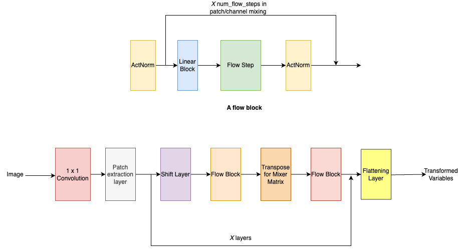
Figure 4: MixerFlow architecture

In summary, we apply the same channel flow to all rows of the mixer-matrix and the same patch flow to all columns of the mixer-matrix. This configuration ensures the desired parameter sharing across the model. These flows, both channel-flows and patch-flows, are seamlessly integrated into our architecture, with each comprising a series of subsequent components. (refer to Figure 4 for an illustration)

Shift layer:

In the MLP-Mixer, the patch definition remains static across the entire architecture, albeit projected into a lower dimension $c$ at the outset—an operation constrained by invertibility concerns. Whilst this approach suits the MLP-Mixer, it introduces grid-like artefacts when applied to sampled images in our MixerFlow model.

To address this issue, shift layers reshape the mixer-matrix back into its original image dimensions. It then creates a frame, leaving the inner part as $(s_{h}:h-p_{h}+s_{h},s_{w}:w-p_{w}+s_{w})$, where $(p_{h},p_{w})$ denotes the patch resolution, $(s_{h},s_{w})$ denotes the shifting unit, and $(h,w)$ corresponds to the image resolution. Subsequently, we re-transform the inner part into an input resembling a mixer-matrix, which we refer to as the “shifted-mixer-matrix.” This process effectively shifts the patch extraction by $(s_{h},s_{w})$ units both vertically and horizontally respectively compared to the old patch definition. This frame carving reduces the number of patches as some input variables are omitted by extraction of the frame. A full mixer layer is applied to the shifted-mixer-matrix, and after this layer, the carved-out frame is reintroduced for the next stage. This strategy ensures robust interactions near the boundaries.

Importantly, the alteration in patch definition has no adverse impact on performance, as neighbouring pixels exhibit a high correlation. Moreover, it facilitates the distribution of transformations for the variables within the carved-out frame, with a focus on the non-carved-out-frame layers. In preliminary experiments we found these shift layers to result in improvements both qualitatively and quantitatively.

Linear block:

As previously mentioned, a coupling layer operates exclusively on approximately half of the input dimensions, underscoring the importance of partition selection. RealNVP (Dinh et al.,, 2017) introduced alternating patterns, which, in certain cases, introduce an order bias. In contrast, Glow (Kingma and Dhariwal,, 2018) advocated for $1\times 1$ convolutions in the form of PLU factorisation, with fixed permutation matrix $P$ and optimisable lower and upper triangular matrices $L$ and $U$, providing a more generalised approach to permutations. In our approach, we employ either LU factorisation or RLU, where R is a permutation matrix that reverses the order of dimensions. It is crucial to emphasise the necessity of a linear block that effectively reverses the shuffling before the application of a shift layer which aims to capture the interaction between the patch boundaries. Subsequently, the linear block is followed by a Flow coupling layer.

Flow layer:

After each Linear Block, we incorporate a flow layer into our architecture. Specifically, we employ a standard affine coupling layer as our chosen flow layer, applicable to either a channel flow or a patch flow. Within each flow layer, we use a residual block as the function approximator. In our experiments, we mostly chose a latent dimension of 128 for both the channel-flow-residual-block and the patch-flow-residual-block, along with the GELU (Hendrycks and Gimpel,, 2023) activation function and batch normalisation (Ioffe and Szegedy,, 2015) in the layers of the residual block.

ActNorm layer:

Due to the computation of a full-form Jacobian when applying layer normalisation (Ba et al.,, 2016), we opt for ActNorm (Kingma and Dhariwal,, 2018) as the preferred normalisation technique in our architecture. ActNorm layers are data-dependent initialised layers with an affine transformation that initialises activations to have a mean of zero and a variance of one based on the first batch. In contrast to Glow-based architectures where ActNorm layers are applied only to the channels, we apply ActNorm to all activations after each flow layer and just before the initial linear layer following each transpose operation (i.e., applying a flow layer to columns of the matrix after applying it to the rows or vice versa).

Identity initialisation:

We initialised all linear blocks to perform an identity function. Additionally, we initialise the final layer of each residual block within the flow with zeros to achieve an identity transformation. This approach, as reported by Kingma and Dhariwal, (2018), has been observed to be beneficial for training deeper flow networks

5 Experiments

We conducted an extensive series of experiments encompassing various datasets, varying dataset sizes, and diverse applications. These applications include permutations, classification tasks, and the integration of Masked Autoregressive Flows (Papamakarios et al.,, 2018) into our MixerFlow model. We use uniform dequantisation and thirty MixerFlow layers with a shift of either one or two every fourth layer in our experiments. We use a patch size of four for $32\times 32$ resolution images, and a patch size of eight for $64\times 64$ resolution images and use Adam (Kingma and Ba,, 2017) for optimisation with the default parameters $\beta_{1}=0.90,\beta_{2}=0.999$. More comprehensive details can be found in Table 8.

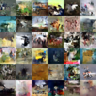
(a) For CIFAR-10

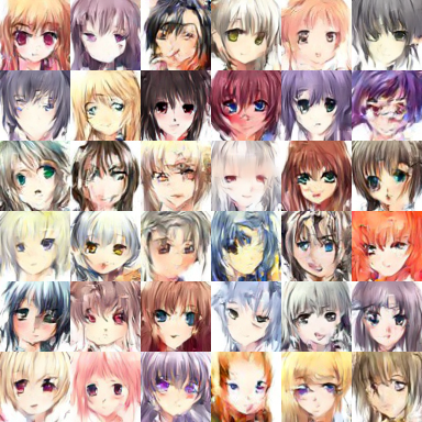
(b) For AnimeFaces

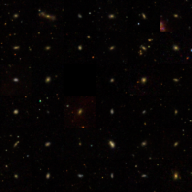
(c) For Galaxy32

Figure 1: Sampled images from our MixerFlow

5.1 Density estimation on $32\times 32$ datasets

Datasets:

In line with previous research, we assessed the performance of MixerFlow on standard $32\times 32$ datasets, specifically ImageNet32 (Russakovsky et al.,, 2015; Van Den Oord et al.,, 2016) and CIFAR-10. (Krizhevsky,, 2009).

Table 1: Negative log-likelihood (in bits per dimension) for $32\times 32$ datasets. Smaller values are better.

Method	CIFAR-10	ImageNet32	Params
Glow	3.51	4.32	11.02M
Neural Spline	3.50	4.24	10.91M
MaCow	3.48	4.34	11.43M
Woodbury	3.48	4.22	11.02M
Emerging	3.48	4.26	11.43M
Periodic	3.49	4.28	11.21M
MixerFlow	3.46	4.20	11.34M

Baselines:

We use various Glow-based baselines for our evaluations: Glow (Kingma and Dhariwal,, 2018), Neural Spline flows (Durkan et al.,, 2019), MaCow (Ma et al.,, 2019), Woodbury (Lu and Huang,, 2021), and Emerging and Periodic convolutions (Hoogeboom et al.,, 2019).

Results:

For a fair comparison, we keep the number of parameters for all models at roughly the same size and train all models with equivalent hyperparameter evaluation. Table 1 presents our quantitative results, demonstrating that MixerFlow outperforms all of the aforementioned baselines. Our scores are worse than those reported in prior works because we use smaller models and train each model on a single GPU. The sample images from our MixerFlow trained on CIFAR-10 can be seen in Figure 1(a).

5.2 Density estimation on $64\times 64$ datasets

Datasets:

We assessed the performance of MixerFlow on two distinct datasets: ImageNet64 (Russakovsky et al.,, 2015), a standard vision dataset, and AnimeFace (Naftali et al.,, 2023), a collection of Anime faces.

Table 2: Negative log-likelihood (in bits per dimension) for $64\times 64$ datasets. Smaller values are better.

Method	AnimeFaces	ImageNet64	Params
Glow	3.21	3.94	37.04M
Neural Spline	3.23	3.95	38.31M
MixerFlow	3.17	3.92	18.90M

Baselines:

For our evaluations, we use a couple of Glow-based baselines, specifically Glow (Kingma and Dhariwal,, 2018), and Neural Spline (Durkan et al.,, 2019).

Results:

Our quantitative results in Table 2 illustrate that MixerFlow outperforms the selected baselines in terms of negative log-likelihood measured in bits per dimension. We considered models with smaller sizes than those in prior works. Notably, our analysis of model sizes reveals that MixerFlow scales remarkably well as image size increases, requiring approximately half the number of parameters compared to the other baselines. This outcome aligns with our expectations, as the hidden patch-flow-MLP dimension remains independent of the number of patches, and the hidden-channel-flow-MLP dimension remains independent of the number of channels—a characteristic inherited from the MLP-Mixer architecture. For a visual representation of our results, please refer to Figure 1(b), which displays sample images generated by our MixerFlow model trained on the AnimeFace dataset.

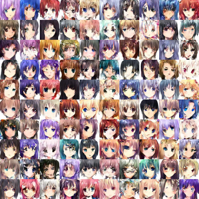
Figure 5: AnimeFace samples from Glow, it is easy to see many artefacts in Glow generation but not in MixerFlow generation

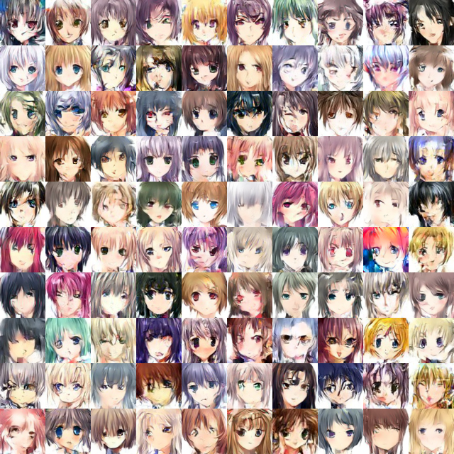
Figure 6: AnimeFaces samples from our model

In the context of the AnimeFaces dataset, we also observed a qualitative improvement. Specifically, we noted a reduction in artefacts compared to the Glow-based baseline (Figure 5 and Figure 6).

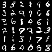
Figure 2: Sampled Images for our MAF-based MixerFlow on MNIST

5.3 Enhancing MAF with the MixerFlow

Masked Autoregressive Flows (MAF) (Papamakarios et al.,, 2018) represent one of the most popular density estimators for tabular data. They are a generalisation of coupling layer flows, such as Glow and RealNVP. Notably, MAF tends to outperform coupling layer flows on tabular datasets, although it comes at the cost of relatively slow generation. The concept of MAF emerged as an approach to enhance the flexibility of the autoregressive model, MADE (Germain et al.,, 2015), by stacking their modules together. This innovation, which enables density evaluations without the typical sequential loop inherent to autoregressive models, significantly accelerated the training process and enabled parallelisation on GPUs.

However, MAF is vulnerable to the curse of dimensionality, necessitating an enormous number of parameters to achieve scalability for image modelling. This requirement for many additional layers can render MAF impractical for certain tasks. In our work, we demonstrate that by substituting a coupling layer with the generalised MAF layer within our MixerFlow model, we can enable MAF for density estimation tasks involving image datasets. This integration leverages the effective weight-sharing architecture inherent in MixerFlow and substantially enhances the performance of the MAF model.

Datasets:

We assessed the performance of the MAF integration on two distinct datasets: MNIST (Deng,, 2012) and CIFAR-10 (Krizhevsky,, 2009).

Table 3: Negative log-likelihood (in bits per dimension) for MAF’s integration into MixerFlow. Smaller values are better.

Method	MNIST	CIFAR-10
MADE	2.04	5.67
MAF	1.89	4.31
Ours	1.22	3.44

Baselines:

We considered MAF (Papamakarios et al.,, 2018) and MADE (Germain et al.,, 2015) as the baselines for our evaluation as they are pre-cursors of MAF’s integration into our architecture.

Results:

Our findings, as presented in Table 3, showcase the density estimation results with MixerFlow further enhancing the use of the MADE module through MAF’s integration in our architecture for MNIST and CIFAR-10. Furthermore, Figure 2 provides a visual representation of the generated samples from our enhanced MAF model on the MNIST dataset

5.4 Datasets with specific permutations

Whilst Glow-based models exhibit expressive capabilities in capturing image dynamics, they heavily rely on convolution operations involving neighbouring pixels to transform the distribution. In contrast, our MixerFlows use multi-layer perceptrons as function approximators, making them invariant to changes in pixel locations within patches and patch locations in the image. This might be helpful if there is some data corruption that induces permutation as Glow-based architectures will result in poor density estimation in such cases. In this section, we empirically demonstrate this advantage across various datasets.

5.4.1 Density estimation on permuted image datasets

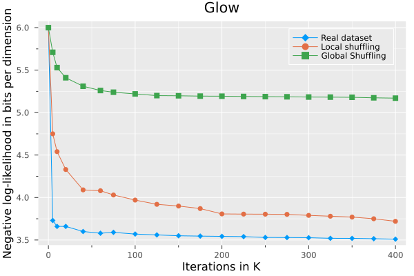
(a) For Glow

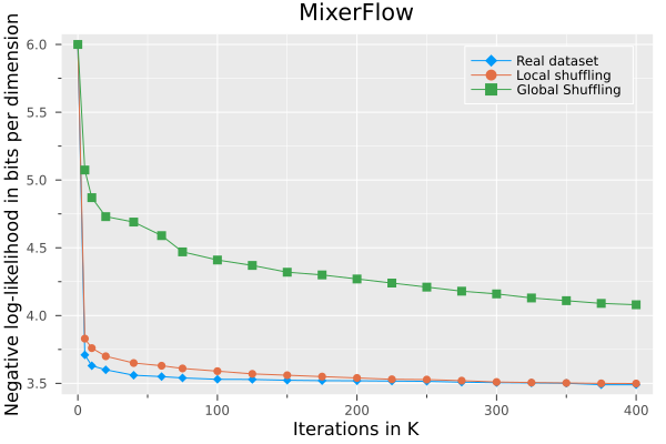
(b) For MixerFlow

Figure 3: Negative log-likelihood (in bits per dimension) comparisons on CIFAR-10 training iterations

Dataset:

Our experimentation involved two types of artificial permutations. Firstly, we divided the input image into patches and performed permutations on both the order of these patches and the pixels within each patch, using a shared permutation matrix. Subsequently, we reorganised these shuffled patches in the image form, referring to this process as “local shuffling.” This setup is analogous to the pixel shuffling experiment introduced by Tolstikhin et al., (2021), but adapted to the case of density estimation. Secondly, we applied a “global shuffling”, where we shuffled all the pixels of the entire image using the same permutations across all images. We created these modified versions of the CIFAR-10 and ImageNet32 datasets, both of which are $32\times 32$ in size.

Table 4: Negative log-likelihood (in bits per dimension) for the global shuffling experiment. Smaller values are better.

Global shuffling	CIFAR-10	Imagenet32	Params
Glow	5.18	5.27	44.24M
Neural Spline	5.01	5.32	89.9M
MixerFlow	4.09	4.91	11.43M
ButterflyFlow	5.11	6,18	-

Baselines:

To assess the performance of our model, we compared it with Glow (Kingma and Dhariwal,, 2018) and Neural Spline flow (Durkan et al.,, 2019). Additionally, we included a comparison with Butterfly Flows (results taken from existing literature) (Meng et al.,, 2022), which are theoretically guaranteed to be able to represent any permutation matrix. All the baselines use the same Glow backbone. Notably, we evaluated larger models for the baselines in this experiment, highlighting that even with larger models, their performance lags in the presence of permutations.

Results:

We tested our hypothesis that MixerFlow is more effective when dealing with permutations in the dataset. The performance gap is substantial for both types of permutations applied to the dataset, as evident from Table 5 and Table 4, where we report lower negative log-likelihoods in bits per dimension (BPD). Figure 3(a) and Figure 3(b) illustrate the training curve for both types of permutations on CIFAR-10. Notably, stronger inductive biases in Glow-based architectures are highly dependent on the order of pixels, resulting in a significant performance drop compared to the original order of image pixels. Conversely, the performance drop is relatively minimal for MixerFlow. Whilst it was intuitively expected that there would be no performance difference on local shuffling datasets, there is a slight difference in the negative log-likelihood, this is due to our shift layer, which requires that neighbouring patches maintain the same structural positions as in the original image.

Table 5: Negative log-likelihood (in bits per dimension) for the local shuffling experiment. Smaller values are better.

Local shuffling	CIFAR-10	Imagenet32	Params
Glow	4.06	4.49	44.24M
Neural Spline	3.99	4.54	89.9M
MixerFlow	3.49	4.24	11.43M

5.4.2 Density estimation on a structured dataset: Galaxy32

Dataset:

Real-world datasets often exhibit unique structures, such as permutations or periodicity. To enhance the robustness of our experiments, we applied MixerFlow to a real world dataset—the Galaxy dataset. This dataset, curated by Ackermann et al., (2018), comprises images of merging and non-merging galaxies. Given that stars can appear anywhere in these images, they exhibit permutation invariance. Additionally, the dataset demonstrates periodicity, as it represents snapshots of a spatial continuum rather than individual isolated images. We downsampled the dataset to a resolution of $32\times 32$ for our experiments.

Baselines:

In our evaluation, we compared the performance of MixerFlow against two baseline models: Glow (Kingma and Dhariwal,, 2018) and Neural Spline (Durkan et al.,, 2019).

Results:

The results, presented in Table 6, clearly indicate that MixerFlow outperformed the chosen baselines. Figure 1(c) showcases samples generated by the MixerFlow model.

Table 6: Negative log-likelihood (in bits per dimension) for the Galaxy32 dataset. Smaller values are better.

Method	Galaxy32
Glow	2.27
Neural Spline	2.25
MixerFlow	2.22

5.5 Hybrid modelling

Nalisnick et al., (2019) introduce a hybrid model that combines a normalising flow model with a linear classification head. This hybrid approach offers a compelling advantage for predictive tasks, as it allows for the computation of both $p(\text{data})$ and $p(\text{label}|\text{data})$ using a single network. This capability enables semi-supervised learning and out-of-distribution detection. However, achieving optimal results often requires joint objective optimization or separate training for different components, as the objective function not only maximises log-likelihood but also minimises predictive error. Significantly over-weighting the predictive error term is sometimes necessary for achieving superior discriminative performance. Since our MixerFlow is based on a discriminative architecture, namely MLP-Mixer, we posit that our model can perform better under similar predictive loss weighting.

Dataset:

We used the CIFAR-10 dataset for the downstream task of classification.

Baselines:

We evaluated the performance of MixerFlow embeddings against two baseline models’ embeddings: Glow and Neural Spline.

Results:

In our experiments, we used our pre-trained models and added a classifier head to them. During training, we kept the flow parameters fixed whilst training the additional linear layer parameters. This setup effectively leveraged the representations learned by the flow models for downstream tasks. Our results in Table 7 indicate that the MixerFlow model exhibited lower losses compared to the chosen baselines. This suggests that MixerFlow embeddings capture more informative representations.

Table 7: Classification loss and accuracy on CIFAR-10 when employing flow-based embeddings

Method	Loss	Accuracy
Glow	1.69	41.23%
Neural Spline	1.67	41.27%
MixerFlow	1.54	45.11%

6 Conclusion and limitations

In this work, we have introduced MixerFlow, a novel flow architecture that draws inspiration from the MLP-Mixer architecture (Tolstikhin et al.,, 2021) designed for discriminative vision tasks. Our experimental results have demonstrated that MixerFlow consistently outperforms or competes comparatively (in terms of negative log-likelihood) with existing models on standard datasets. Importantly, it exhibits good scalability, making it suitable for handling larger image sizes. Additionally, the integration of MAF layers (Papamakarios et al.,, 2018) into our architecture showed considerable improvements in MAF, showcasing its adaptability and versatility for integrating normalising flow architectures beyond coupling layers.

We also explored the application of MixerFlow to datasets featuring artificial permutations and structured permutations, underlining its practicality and wide-ranging utility. To conclude, our work has highlighted the potential of the acquired representations in the downstream classification task on CIFAR-10, as evidenced by lower loss values.

One limitation of our proposed architecture is the absence of strong inductive biases typically associated with convolution-based flows. This may be especially relevant if little training data is available.

7 Future work and broader impact

Whilst our experimental analysis focuses on MixerFlow with MLP-based neural networks, it is crucial to note that MixerFlow’s architecture is not restricted to specific neural network types or flow networks. It enables parameter sharing and can be adapted to various network architectures. This adaptability extends to the incorporation of residual flows (Chen et al.,, 2020), attention layers (Sukthanker et al.,, 2022), and convolutional layers, especially for larger image sizes and patch sizes, offering the potential for enhanced inductive biases and parameter sharing. Additionally, the inclusion of glow-like layers before applying the MixerFlow layers could further strengthen inductive biases.

Another promising avenue for improvement is enabling multiscale design (Kingma and Dhariwal,, 2018), a well-established technique for boosting the performance of flow-based models. We leave the integration of multi-scale architecture, and stronger inductive biases for future work, believing it could further enhance the MixerFlow architecture’s capabilities. We are optimistic about the potential of MixerFlow to advance flow-based image modelling, and we hope for more developments in architectural backbone research for flow models in the future.

Acknowledgements

We are grateful to the HPI Data Science and Engineering Research School for funding this research. Additionally, we extend our gratitude to Arkadiusz Kwasigroch, Sumit Shekhar, and Thomas Gaertner for their feedback on an earlier draft.

 

Supplementary Material

 

8 Additional experimental details for our method

We employed the Adam optimiser exclusively for all our experiments. The learning is chosen $\in[0.001,0.0005]$, $\beta_{1}=0.90,\beta_{2}=0.999$. We used Cosine decay for all experiments with the minimum learning rate equalling zero. In initial experiments, we found that 30 mixer layers with a shift layer every four layers and four flow layers for both, channel-mixing and patch-mixing, performed satisfactorily and we persisted with it for all of the experiments. We used an NVIDIA a100 GPU for training in our experiments. For more comprehensive information, please refer to Table 8.

Table 8: Model Architectures and hyperparameters for our method.

Datasets
		CIFAR-10	Imagenet32	Galaxy32	Imagenet64	AnimeFaces	MNIST
	Resolution	32	32	32	64	64	28
	Training Points	48,000	1,229,904	5,000	1,229,904	61,023	57,600
	type	coupling	coupling	coupling	coupling	coupling	autoregressive
	layers	30	30	30	30	30	30
	patch size	4	4	4	8	8	4
	hidden dimension	128	128	64	128	128	64
	shift layer	1	1	1	2	2	None
	Linear block	LU	LU	LU	LU	LU	RLU
	grad clip	5.0	5.0	5.0	5.0	5.0	5.0
	learning rate(lr)	0.001	0.001	0.001	0.0005	0.0005	0.0005
	$\beta_{1}$	0.90	0.90	0.90	0.90	0.90	0.90
	$\beta_{2}$	0.999	0.999	0.999	0.999	0.99	0.999
	training steps	400K	500K	50K	400K	400K	400K
	batch size	512	512	512	200	200	512

9 Ablation studies

In this section, we show ablation studies showing the effect of the components we have added to our architecture. We chose a basic architecture, which does not have any linear block, shifting layer, and only 30 mixer layers, as a baseline and show how different components affect the results. We make all the evaluations on CIFAR-10.

Our experiments in Table 9 confirm that adding linear blocks and shift layers helped improve density estimation by a huge margin. Additionally, our result with 60 layers indicates stronger performance as the number of layers gets larger for our architecture.

Table 9: Negative log-likelihood (in bits per dimension) Smaller values are better.

Additions	BPD
Baseline	3.81
60 layers	3.52
Linear blocks	3.49
Shift layers	3.58

10 Things that did not help

Shift layer with larger shifts:

In our experimentation with $32\times 32$ datasets, we explored the use of larger shifts and more frequent applications of the shift layer. Whilst these modifications proved to be advantageous compared to not using a shift layer at all, they did not yield great improvements when the shift exceeded a value of 1 for these particular datasets. We believe that the mixing requires many layers and the introduction of larger shifts significantly alters the patch definitions of small-resolution images leading to sub-par results.

Stripes, bands, or dilated patches

: Instead of using simple non-overlapping patches, we experimented with stripes, bands, and dilated patches. However, this did not result in any noticeable improvement.

Changing the patch size mid-layers

: We conducted experiments involving the use of different patch sizes within different layers of our model. Specifically, we experimented with smaller-resolution patches in earlier layers, followed by higher-resolution patches (and vice versa). The intention behind this approach was to enable the model to initially learn broader features and progressively refine specific features, similar to the behaviour of convolutional layers. However, this change in patch size did not lead to any noticeable improvements. Additionally, using dilated patches did not yield any performance enhancements.

Squeezing operation

: Following Glow, we tried the squeeze layers to change the spatial resolution into channel dimension. Unfortunately, it led the models to overfit easily as the training loss went down but the validation loss went up.

Iterative growing of flows:

We experimented with deeper architectures by first training only a more shallow architecture. After several epochs, we added more layers with identity initialisation and repeated the process until the desired architecture depth was achieved. We also worked with different learning rate sizes for different layers. However, we found no improvement compared to a simple end-to-end training scheme.

Training instabilities:

We tried to enhance training stabilities by replacing the affine scale functions – traditionally an exponential function – with functions bounded away from 0. We also tried replacing the Gaussian base distribution with fat-tailed distributions such as a Cauchy distribution or a Gaussian mixture spike and slab model.

Positional embedding:

In early iterations, we tried incorporating either learnable or sinusoidal positional embeddings as conditioning variables into the flow networks but found them to only add unnecessary complexity.

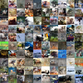
Figure 7: CIFAR-10 samples from our model

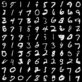
Figure 8: MNIST samples from our model

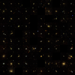
Figure 9: Galaxy32 samples from our model

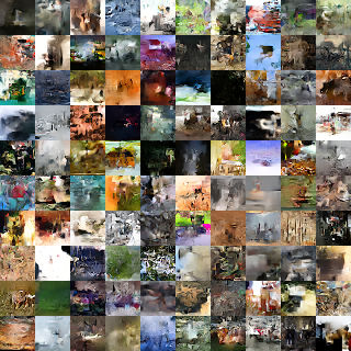
Figure 10: Imagenet32 samples from our model

References

- Ackermann et al., (2018) Ackermann, S., Schawinski, K., Zhang, C., Weigel, A. K., and Turp, M. D. (2018). Using transfer learning to detect galaxy mergers. Monthly Notices of the Royal Astronomical Society, 479(1):415–425.
- Ahn et al., (2022) Ahn, B., Kim, C., Hong, Y., and Kim, H. J. (2022). Invertible monotone operators for normalizing flows. Advances in Neural Information Processing Systems, 35:16836–16848.
- Ba et al., (2016) Ba, J. L., Kiros, J. R., and Hinton, G. E. (2016). Layer normalization.
- Behrmann et al., (2019) Behrmann, J., Grathwohl, W., Chen, R. T. Q., Duvenaud, D., and Jacobsen, J.-H. (2019). Invertible residual networks.
- Chen et al., (2020) Chen, R. T. Q., Behrmann, J., Duvenaud, D., and Jacobsen, J.-H. (2020). Residual flows for invertible generative modeling.
- Dai and Seljak, (2020) Dai, B. and Seljak, U. (2020). Sliced iterative normalizing flows. In International Conference on Machine Learning.
- Dao et al., (2020) Dao, T., Gu, A., Eichhorn, M., Rudra, A., and Ré, C. (2020). Learning fast algorithms for linear transforms using butterfly factorizations.
- Deng, (2012) Deng, L. (2012). The mnist database of handwritten digit images for machine learning research. IEEE Signal Processing Magazine, 29(6):141–142.
- Dinh et al., (2017) Dinh, L., Sohl-Dickstein, J., and Bengio, S. (2017). Density estimation using real nvp.
- Dosovitskiy et al., (2021) Dosovitskiy, A., Beyer, L., Kolesnikov, A., Weissenborn, D., Zhai, X., Unterthiner, T., Dehghani, M., Minderer, M., Heigold, G., Gelly, S., Uszkoreit, J., and Houlsby, N. (2021). An image is worth 16x16 words: Transformers for image recognition at scale.
- Durkan et al., (2019) Durkan, C., Bekasov, A., Murray, I., and Papamakarios, G. (2019). Neural spline flows.
- English et al., (2023) English, E., Kirchler, M., and Lippert, C. (2023). Kernelized normalizing flows.
- Finzi et al., (2019) Finzi, M., Izmailov, P., Maddox, W., Kirichenko, P., and Wilson, A. G. (2019). Invertible convolutional networks. In Workshop on Invertible Neural Nets and Normalizing Flows, International Conference on Machine Learning, volume 2.
- Germain et al., (2015) Germain, M., Gregor, K., Murray, I., and Larochelle, H. (2015). Made: Masked autoencoder for distribution estimation.
- Grathwohl et al., (2018) Grathwohl, W., Chen, R. T. Q., Bettencourt, J., Sutskever, I., and Duvenaud, D. (2018). Ffjord: Free-form continuous dynamics for scalable reversible generative models.
- He et al., (2015) He, K., Zhang, X., Ren, S., and Sun, J. (2015). Deep residual learning for image recognition.
- Hendrycks and Gimpel, (2023) Hendrycks, D. and Gimpel, K. (2023). Gaussian error linear units (gelus).
- Ho et al., (2019) Ho, J., Chen, X., Srinivas, A., Duan, Y., and Abbeel, P. (2019). Flow++: Improving flow-based generative models with variational dequantization and architecture design. In International Conference on Machine Learning, pages 2722–2730. PMLR.
- Hoogeboom et al., (2019) Hoogeboom, E., van den Berg, R., and Welling, M. (2019). Emerging convolutions for generative normalizing flows.
- Ioffe and Szegedy, (2015) Ioffe, S. and Szegedy, C. (2015). Batch normalization: Accelerating deep network training by reducing internal covariate shift.
- Karami et al., (2019) Karami, M., Schuurmans, D., Sohl-Dickstein, J. N., Dinh, L., and Duckworth, D. (2019). Invertible convolutional flow. In Neural Information Processing Systems.
- Kingma and Ba, (2017) Kingma, D. P. and Ba, J. (2017). Adam: A method for stochastic optimization.
- Kingma and Dhariwal, (2018) Kingma, D. P. and Dhariwal, P. (2018). Glow: Generative flow with invertible 1x1 convolutions.
- Kingma and Welling, (2022) Kingma, D. P. and Welling, M. (2022). Auto-encoding variational bayes.
- Kobyzev et al., (2021) Kobyzev, I., Prince, S. J., and Brubaker, M. A. (2021). Normalizing flows: An introduction and review of current methods. IEEE Transactions on Pattern Analysis and Machine Intelligence, 43(11):3964–3979.
- Krizhevsky, (2009) Krizhevsky, A. (2009). Learning multiple layers of features from tiny images.
- Laparra et al., (2011) Laparra, V., Camps-Valls, G., and Malo, J. (2011). Iterative gaussianization: From ICA to random rotations. IEEE Transactions on Neural Networks, 22(4):537–549.
- Lee et al., (2021) Lee, K., Chang, H., Jiang, L., Zhang, H., Tu, Z., and Liu, C. (2021). Vitgan: Training gans with vision transformers.
- Lu and Huang, (2021) Lu, Y. and Huang, B. (2021). Woodbury transformations for deep generative flows.
- Ma et al., (2019) Ma, X., Kong, X., Zhang, S., and Hovy, E. (2019). Macow: Masked convolutional generative flow.
- Meng et al., (2020) Meng, C., Song, Y., Song, J., and Ermon, S. (2020). Gaussianization flows.
- Meng et al., (2022) Meng, C., Zhou, L., Choi, K., Dao, T., and Ermon, S. (2022). ButterflyFlow: Building invertible layers with butterfly matrices. In Chaudhuri, K., Jegelka, S., Song, L., Szepesvari, C., Niu, G., and Sabato, S., editors, Proceedings of the 39th International Conference on Machine Learning, volume 162 of Proceedings of Machine Learning Research, pages 15360–15375. PMLR.
- Naftali et al., (2023) Naftali, M. G., Sulistyawan, J. S., and Julian, K. (2023). Aniwho : A quick and accurate way to classify anime character faces in images.
- Nalisnick et al., (2019) Nalisnick, E., Matsukawa, A., Teh, Y. W., Gorur, D., and Lakshminarayanan, B. (2019). Hybrid models with deep and invertible features.
- O’Shea and Nash, (2015) O’Shea, K. and Nash, R. (2015). An introduction to convolutional neural networks.
- Papamakarios et al., (2021) Papamakarios, G., Nalisnick, E., Rezende, D. J., Mohamed, S., and Lakshminarayanan, B. (2021). Normalizing flows for probabilistic modeling and inference.
- Papamakarios et al., (2018) Papamakarios, G., Pavlakou, T., and Murray, I. (2018). Masked autoregressive flow for density estimation.
- Peters and Herrmann, (2019) Peters, B. and Herrmann, F. J. (2019). Generalized minkowski sets for the regularization of inverse problems.
- Russakovsky et al., (2015) Russakovsky, O., Deng, J., Su, H., Krause, J., Satheesh, S., Ma, S., Huang, Z., Karpathy, A., Khosla, A., Bernstein, M., Berg, A. C., and Fei-Fei, L. (2015). Imagenet large scale visual recognition challenge.
- Sukthanker et al., (2022) Sukthanker, R. S., Huang, Z., Kumar, S., Timofte, R., and Gool, L. V. (2022). Generative flows with invertible attentions.
- Tolstikhin et al., (2021) Tolstikhin, I., Houlsby, N., Kolesnikov, A., Beyer, L., Zhai, X., Unterthiner, T., Yung, J., Steiner, A., Keysers, D., Uszkoreit, J., Lucic, M., and Dosovitskiy, A. (2021). Mlp-mixer: An all-mlp architecture for vision.
- Van Den Oord et al., (2016) Van Den Oord, A., Kalchbrenner, N., and Kavukcuoglu, K. (2016). Pixel recurrent neural networks. In International conference on machine learning, pages 1747–1756. PMLR.
- van den Oord et al., (2016) van den Oord, A., Kalchbrenner, N., Vinyals, O., Espeholt, L., Graves, A., and Kavukcuoglu, K. (2016). Conditional image generation with pixelcnn decoders.
- Witte et al., (2021) Witte, P. A., Louboutin, M., Siahkoohi, A., Rizzuti, G., Peters, B., and Herrmann, F. J. (2021). Invertiblenetworks.jl - memory efficient deep learning in julia. In JuliaCon. (JuliaCon, virtual).