Electronic Goos–Hänchen shift through double barriers in phosphorene

Abstract

We consider fermions in phosphorene through double barriers and study the corresponding Goos-Hänchen (GH) shift. To accomplish this, we initially compute the corresponding transmission amplitude by applying boundary conditions. From the resulting transmission phase, we extract the GH shift. Our findings reveal that the GH shift’s magnitude is contingent upon the energy of the incident electron and the barrier parameters. Additionally, we observe that the GH shift changes sign at the transmission boundaries—specifically, at the transmission resonances occurring immediately before and after the gap region, where transmission is zero.

I Introduction

A monolayer of black phosphorus is called phosphorene, it can be exfoliated down to extremely thin layers. The phosphorus (P) atoms are arranged in a hexagonal staggered lattice. This is a layered material, similar to graphite and transition metal dichalcogenides (TMDs), where each atomic layer is bound to adjacent ones by weak Van Der Waals interactions, enabling the isolation of a few atomic layer thin films via mechanical exfoliation [1, 2, 3]. The intrinsic anisotropy of phosphorene is observed in its optical, thermal, electrical, and mechanical properties, which makes it an intriguing material with potential applications in devices based on thermoelectronic, spintronic, and electronic effects. In contrast to TMDs and graphene, phosphorene exhibits an intrinsic direct band gap that is layer-dependent and varies between $0.3$ eV (for bulk) and $2$ eV (for single layer) [4]. It was also observed that the layer thickness of phosphorene has a substantial effect on the time response ratios for ON/OFF, OFF, and ON currents in phosphorene field effect transistors (FETs) [2].

In recent years, significant advances have been made in the study of electronic transport properties within graphene systems [5]. As an example, we cite the quantum version of the Goos-Hänchen effect, originating from the complete reflection of particles at the interfaces between two distinct media. It was first observed by Hermann Fritz Gustav Goos and Hilda Hänchen [6, 7], the Goos-Hänchen (GH) shift was theoretically explained by Artman in the late 1940s [8]. Numerous studies focusing on various graphene-based nanostructures, such as single barrier [9], double barrier [10], and superlattices [11], have indicated that GH shifts can be amplified through transmission resonances. Additionally, these shifts can be controlled by adjusting the electrostatic potential and induced gap [9]. Similarly to semiconductors, electric and magnetic barriers can modulate GH shifts in graphene, akin to observations in atomic optics [12, 13]. Crucially, research has highlighted the pivotal role played by GH shifts in determining the group velocity of quasiparticles along interfaces of graphene p-n junctions [14, 15]. Furthermore, investigations have revealed that the valley-dependent GH effect in strained graphene leads to varying group velocities for electrons near the K and K’ valleys [16].

Similarly to other systems, investigations of the potential enhancement, mainly through resonance phenomena, of the GH shift in phosphorene through theoretical analysis have been reported recently [17]. Specifically, for electrons encountering various potential barriers in phosphorene, the GH shifts and transmission coefficients were analyzed. A transfer matrix approach was employed, considering current conservation and the non-hermiticity issue in the envelope effective equation due to sharp boundaries. The results indicated that the GH shifts strongly depend on the type of barrier and incident angle. Most importantly, these GH shifts are substantial and detectable, and in fact, they surpass those observed previously in graphene. Very recently, we investigated the transport properties of massive charge carriers in phosphorene scattered through double barriers [18]. We examined the influence of potential barrier parameters and the wave vector of incident particles in the $x$-direction on the energy spectrum. Employing appropriate boundary conditions and the transfer matrix method, we calculated the transmission coefficient and conductance. These values were thoroughly analyzed to discern the fundamental characteristics of our system, including their dependency on physical parameters and the armchair boundary condition. Our results provided strong evidence for the pronounced anisotropy of phosphorene and verified the occurrence of Klein tunneling at normal incidence. Furthermore, under specific circumstances, we observed oscillatory patterns in transmission and conductance concerning the barrier width.

We study the effect of double barriers on the GH shift in phosphorene along the lines of our earlier work [18]. In fact, depending on the phase shifts, we have determined the GH shifts, which are very sensitive to the physical parameters of the system under consideration. To give a comprehensive analysis of our findings, we provide a numerical analysis of the GH shift associated with the transmission probability under various conditions. More specifically, we demonstrated that the GH shifts could have both a negative and a positive sign, depending on the choice of parameters. Our findings also indicate that the system’s characteristics can be used to control the GH shift, both in magnitude and sign.

The organization of the present paper is as follows: In Sec. II, we develop our mathematical model and define the system Hamiltonian, and then, by solving our stationary wave equation in each region of space, we derive the corresponding energy spectrum of our system. Then we calculate the transmission probability and deduce the associated phase shift, which is then used to derive the corresponding GH shifts in Sec. III. By carefully selecting the system physical parameters, we numerically compute the GH phase shift and transmission, which were then considered to discuss the basic features of our system in Sec. IV. Finally, we summarize our findings and conclude.

II Theoretical Model

We consider fermions living on a piece of phosphorene subjected to double barriers, as depicted in Fig. 1. This piece is composed of five regions labeled by the index $j=1,\cdots,5$. The incident charged particle beam with energy $E$ and incident angle $\phi$ is coming from the input region $(j=1)$, at the extreme left of Fig. 1. The transmitted charged particle beam is then detected in the output region $(j=5)$ with a lateral shift $S_{t}$, called the GH shift. The strengths of the static square potential barrier $V_{j}(x)$ are given by

$$V_{j}(x)=\left\{\begin{array}[]{llll}{V_{1}=V},&\qquad{0<x<d_{1}}\\ {V_{2}=0},&\qquad{d_{1}<x<d_{1}+d_{2}}\\ {V_{3}=-V},&\qquad{d_{1}+d_{2}<x<d}\\ {0},&\qquad\mbox{otherwise}.\end{array}\right.$$ (1)

The width of the scattering region is defined to be $d=d_{1}+d_{2}+d_{3}$, with $d_{1}=d_{3}=\frac{1-q_{2}}{2}d$ and $d_{2}=q_{2}d$, as shown in Fig. 1.

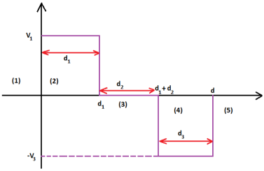
Figure 1: (color online) Diagram illustrating the potential $V(x)$ of the phosphorene double barriers, which has two amplitudes $(V_{1},0,V_{3})$, each of which corresponds to a distinct region $j$ width $d_{j}$, defining the total width by $d=(d_{1}+d_{2}+d_{3})$.

By expanding the effective Hamiltonian around the high symmetry point $k=0$ ($\Gamma$ point) and keeping only second-order terms in $k$, it can be shown that the long-wavelength approximation for the Hamiltonian for the monolayer phosphorene can be written as follows [19, 20, 18]

$$H=\begin{pmatrix}u_{0}+\eta_{x}k_{x}^{2}+\eta_{y}k_{y}^{2}&\delta+\gamma_{x}k_{x}^{2}+\gamma_{y}k_{y}^{2}+i\chi k_{x}\\ \delta+\gamma_{x}k_{x}^{2}+\gamma_{y}k_{y}^{2}-i\chi k_{x}&u_{0}+\eta_{x}k_{x}^{2}+\eta_{y}k_{y}^{2}\\ \end{pmatrix}$$ (2)

where the parameters involved are ${u}_{0}=-0.42$ eV, $\eta_{{x}}=0.58$ eV Ų, $\eta_{{y}}=1.01$ eV Ų, $\delta=0.76$ eV, $\chi=5.25$ eV Å, $\gamma_{{x}}=3.93$ eV Ų and $\gamma_{{y}}=3.83$ eV Å. We combine the scattering potential (1) and the effective Hamiltonian (2) to write our wave equation in each region $j$ using the total Hamiltonian

$$H_{j}=H+V_{j}(x)\mathbb{I}_{2}$$ (3)

where $\mathbb{I}_{2}$ is the unit matrix. From the stationary eigenvalue equation $H_{j}\Psi_{j}=E_{j}\Psi_{j}$ for spinor $\Psi_{j}$, one can show that the dispersion relation takes the following form

$$E_{j}=V_{j}+u_{0}+\eta_{x}k_{j}^{2}+\eta_{y}k_{y}^{2}+s_{j}\sqrt{\left(\delta+\gamma_{x}k_{j}^{2}+\gamma_{y}k_{y}^{2}\right)^{2}+\left(\chi k_{j}\right)^{2}}$$ (4)

with $s_{j}={\mbox{sgn}}{\left(E-V_{j}-u_{0}-\eta_{x}k_{x}^{2}-\eta_{y}k_{y}^{2}\right)}$. Using the fact that $u_{0},\delta,k_{j}\gg k_{j}^{2}$ at low momenta, the term proportional to $k_{j}^{2}<1$ could be neglected in the energy spectrum. The longitudinal wave vectors $k_{j}$ corresponding to region 5 are provided by

$$k_{j}=\chi^{-1}\sqrt{\left(E-V_{j}-u_{0}-\eta_{y}k_{y}^{2}\right)^{2}+\left(\delta+\gamma_{y}k_{y}^{2}\right)^{2}}.$$ (5)

Taking into consideration the conservation of the transverse wave vector, $k_{y}$, we can express the spinor wavefunctions of the carriers moving along the $\pm x$-directions as $\Psi_{j}(x,y)=\phi_{j}(x)e^{ik_{y}y}$. Then, in the first region $(j=1,x<0)$ we use the eigenvalue equation to show that the corresponding spinor is given by a linear combination of incident and reflected waves is given by

$$\phi_{1}(x)=\left(\begin{array}[]{c}{1}\\ {z_{1}}\\ \end{array}\right)e^{ik_{1}x}+r\left(\begin{array}[]{c}{1}\\ {z_{1}^{-1}}\\ \end{array}\right)e^{-ik_{1}x}=L_{1}[x]\left(\begin{array}[]{c}{1}\\ {r}\\ \end{array}\right).$$ (6)

Concerning the potential regions $j=2,3,$ and $4$, we obtain the following solutions

$$\phi_{j}(x)=a_{j}\left(\begin{array}[]{c}{1}\\ {z_{j}}\\ \end{array}\right)e^{ik_{j}x}+b_{j}\left(\begin{array}[]{c}{1}\\ {z_{j}^{-1}}\\ \end{array}\right)e^{-ik_{j}x}=L_{j}[x]\left(\begin{array}[]{c}{a_{j}}\\ {b_{j}}\\ \end{array}\right)$$ (7)

and finally in the last region $j=5$, the spinor is given only by the sole transmitted wave

$$\phi_{5}(x)=t\left(\begin{array}[]{c}{1}\\ {z_{1}}\\ \end{array}\right)e^{ik_{1}x}=L_{1}[x]\left(\begin{array}[]{c}{t}\\ {0}\\ \end{array}\right)$$ (8)

where we have defined the following complex numbers

$$z_{j}=s_{j}e^{-i\alpha_{j}},\quad\alpha_{j}=\arctan\left(\frac{\chi k_{j}}{\delta+\gamma_{y}k_{y}^{2}}\right).$$ (9)

We will see how the above solutions to the energy spectrum can be used to deal with different issues regarding the transport properties. In fact, these concern the transmission probability and the corresponding GH shift.

III The Goss-Hänchen Shifts

To derive the Goss-Hänchen (GH) shifts, we first determine the reflection and transmission probabilities. Indeed, using the boundary conditions for the spinors defined in the previous section at various interfaces $(x=x_{1}=0,x_{2}=d_{1},x_{3}=d_{1}+d_{2},x=d$ with $d=d_{1}+d_{2}+d_{3}$), we identify the reflection and the transmission coefficients through the following expression

$$\dbinom{1}{r}={L_{1}}^{-1}[0]\cdot L_{2}[0]\cdot{L_{2}}^{-1}[d_{1}]\cdot L_{3}[d_{1}]\cdot{L_{3}}^{-1}[d_{1}+d_{2}]\cdot L_{4}[d_{1}+d_{2}]\cdot{L_{4}}^{-1}[d]\cdot L_{1}[d]\ \dbinom{t}{0}.$$ (10)

It is then beneficial to define the transfer matrix associated with two barriers as follows

$$\mathcal{M}={L_{1}}^{-1}\cdot[0]\cdot Q\cdot{L_{1}}[d]=\begin{pmatrix}\mathcal{M}_{11}&\mathcal{M}_{12}\\ \mathcal{M}_{21}&\mathcal{M}_{22}\\ \end{pmatrix}$$ (11)

where the matrix $Q$ reads as

$$Q=L_{2}[0]\cdot{L_{2}}^{-1}[d_{1}]\cdot L_{3}[d_{1}]\cdot{L_{3}}^{-1}[d_{1}+d_{2}]\cdot L_{4}[d_{1}+d_{2}]\cdot{L_{4}}^{-1}[d].$$ (12)

From the above definitions, we can rewrite the relationship (10) connecting the input and output in the following elegant manner

$$\dbinom{1}{r}=\mathcal{M}\dbinom{t}{0}$$ (13)

and therefore we can easily identify the transmission and reflection amplitudes as follows

$$t=\frac{1}{\mathcal{M}_{11}},\quad r=\frac{\mathcal{M}_{21}}{\mathcal{M}_{11}}.$$ (14)

For our task, it is convenient to determine the inverse of $t$. After a series of intricate algebraic steps, we eventually derive the expression

$$t^{-1}={\frac{i{{\rm e}^{ik_{{1}}d}}}{2s_{2}\sin^{2}\alpha_{{1}}\sin\alpha_{{2}}\sin\alpha_{{4}}}}\left(\zeta+\vartheta+\varkappa+\varsigma+\tau+\beta\right)$$ (15)

where the quantities involved are defined by

$$\zeta=2\sin\left(d_{{1}}k_{{2}}\right)\sin\left(d_{{2}}k_{{1}}\right)\sin\left(d_{{3}}k_{{4}}\right)\zeta^{+}$$ (16)

$$\zeta^{+}=\sin\alpha_{{1}}\left(is_{{1}}\cos\alpha_{{4}}-is_{{2}}\cos\alpha_{{4}}\cos\alpha_{{1}}\cos\alpha_{{2}}-is_{{4}}\cos\alpha_{{1}}\right)-\cos\alpha_{{2}}s_{{1}}s_{{2}}s_{{4}}\left(\cos\alpha_{{1}}-i\sin\alpha_{{1}}\right)$$ (17)

$$\vartheta=2\sin\alpha_{{4}}\sin\left(d_{{1}}k_{{2}}\right)\sin\left(d_{{2}}k_{{1}}\right)\cos\left(d_{{3}}k_{{4}}\right)\left(-2s_{{1}}\cos\alpha_{{1}}+s_{{2}}\left(\cos\alpha_{{1}}\right)^{2}\cos\alpha_{{2}}+s_{{2}}\cos\alpha_{{2}}\right)$$ (18)

$$\varkappa=2\sin\alpha_{{1}}\sin\left(d_{{1}}k_{{2}}\right)\sin\left(d_{{3}}k_{{4}}\right)\cos\left(d_{{2}}k_{{1}}\right)\left(-s_{{1}}\cos\alpha_{{4}}+s_{{2}}\cos\alpha_{{1}}\cos\alpha_{{4}}\cos\alpha_{{2}}-s_{{4}}\cos\alpha_{{1}}\right)$$ (19)

$$\varsigma=-2s_{{2}}\sin\alpha_{{2}}\cos\left(d_{{1}}k_{{2}}\right)\sin\left(d_{{2}}k_{{1}}\right)\varsigma^{+}$$ (20)

$$\varsigma^{+}=\sin\left(d_{{3}}k_{{4}}\right)\cos\alpha_{{4}}\left(\left(\sin\alpha_{{1}}\right)^{2}+s_{{1}}\cos\alpha_{{1}}s_{{4}}+i\cos\alpha_{{1}}\sin\alpha_{{1}}\cos\left(d_{{3}}k_{{4}}\right)\sin\alpha_{{4}}\right)$$ (21)

$$\tau=-2s_{{2}}\sin\alpha_{{1}}\cos\left(d_{{1}}k_{{2}}\right)\cos\left(d_{{2}}k_{{1}}\right)\sin\left(d_{{3}}k_{{4}}\right)\sin\alpha_{{2}}\left(i\sin\alpha_{{1}}\cos\alpha_{{4}}+s_{{1}}s_{{4}}\right)$$ (22)

$$\beta=-2\sin\alpha_{{1}}\sin\alpha_{{4}}s_{{2}}\cos\left(d_{{2}}k_{{1}}\right)\cos\left(d_{{3}}k_{{4}}\right)\left(i\sin\alpha_{{1}}\sin\left(d_{{1}}k_{{2}}\right)\cos\alpha_{{2}}-\cos\alpha_{{1}}\cos\left(d_{{1}}k_{{2}}\right)\sin\alpha_{{2}}\right).$$ (23)

For a given transverse wave vector $k_{y0}$ that corresponds to the incidence angle $\varOmega_{1}(k_{y0})$, we account for the incident, reflected, and transmitted beams that fall with an incident angle in the range $[0,\pi/2]$, in order to investigate the GH shifts induced by the spatially modulated potential in phosphorene. The incident, reflected, and transmitted beams are then given by

$$\Pi_{i}(x,y)=\int_{-\infty}^{+\infty}g(k_{y}-k_{y0})e^{ikx+ik_{y}y}\dbinom{1}{e^{i\varOmega(k_{y})}}\,dk_{y}$$ (24)

$$\Pi_{r}(x,y)=\int_{-\infty}^{+\infty}r(k_{y})g(k_{y}-k_{y0})e^{-ikx+ik_{y}y}\dbinom{1}{-e^{-i\varOmega(k_{y})}}\,dk_{y}$$ (25)

$$\Pi_{t}(x,y)=\int_{-\infty}^{+\infty}t(k_{y})g(k_{y}-k_{y0})e^{ikx+ik_{y}y}\dbinom{1}{e^{i\varOmega(k_{y})}}\,dk_{y}$$ (26)

where $g(k_{y}-k_{y0})$ is a Gaussian-shaped and single-peaked positive definite function around the primary wave vector $k_{y0}$. It describes the well-collimated incident beam. With the aid of boundary conditions, the reflection $r(k_{y})$ and transmission $t(k_{y})$ can be written in complex notation as follows

$$t=\rho_{t}e^{i\varphi_{t}},\quad r=\rho_{r}e^{i\varphi_{r}}$$ (27)

such that their modulus and the associated phase shifts are given by

$$\rho_{t}=\sqrt{\Re^{2}[t]+\Im^{2}[t]},\quad\rho_{r}=\sqrt{\Re^{2}[r]+\Im^{2}[r]}$$ (28)

$$\varphi_{t}=\arctan\left({i\frac{t^{*}-t}{t+t^{*}}}\right),\quad\varphi_{r}=\arctan\left({i\frac{r^{*}-r}{r+r^{*}}}\right).$$ (29)

At this stage, we can determine the transmission $T$ and reflection $R$ probabilities as

$$T=\rho^{2}_{t},\quad R=\rho^{2}_{r}$$ (30)

and extract the corresponding GH shifts that are just given by the derivatives of the transmission and reflection phase shifts with respect to the transverse momentum $k_{y}$, respectively. Otherwise, we have the following relationships:

$$S_{t}=-\frac{\partial\varphi_{t}}{\partial k_{y}}\Big{|}_{k_{y0}},\quad S_{r}=-\frac{\partial\varphi_{r}}{\partial k_{y}}\Big{|}_{k_{y0}}.$$ (31)

Next, we will explore the aforementioned findings to examine the numerical results for both the transmission and GH shifts. The transmission GH shift is obviously related to variations of transmission phase with respect to the incident angle $\phi$ while the reflection GH shift is related to variations of reflection phase with respect to the incidence angle $\phi$. Since both GH shifts have similar behavior, we have decided to consider only the transmission GH shifts in this work. Specifically, our focus will be on investigating various transmission channels and their responses under different conditions related to various system physical parameters. Additionally, we will highlight the novel aspects of our findings as compared to existing literature.

IV Results and discussions

Fig. 2 illustrates the Goos-Hänchen (GH) shift and the corresponding transmission probability as a function of the incident energy $E$. In our numerical computations, we maintained a fixed incident angle $\phi=4^{\circ}$, a barrier width of $d=10$ nm, and a ratio of $q_{2}=1/3$, while varying the barrier height $V$ for several values. This figure demonstrates a consistent pattern where a positive peak in the GH shift consistently precedes the occurrence of a negative valley, a behavior observed across all barrier height values. Notably, the energies at which the GH shift changes signs align precisely with the points where transmission becomes zero. Specifically, the transmission resonances, which appear just before and just after the transmission gap region, are strongly correlated with the points at which the GH shift undergoes a sign change. We can thus deduce that the GH shift is strongly influenced by the energy $E$, changing sign precisely at transmission resonances located just before or after the zero transmission region. This observation provides a practical method to achieve the desired sign of the GH shift by tuning to the correct energy. It’s worth mentioning that the choice of $\phi=4^{\circ}$ was made because the double barrier GH shift in phosphorene displays distinct resonances at this specific angle.

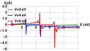
(a)

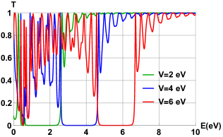
(b)

Figure 2: The GH Shift (a) and transmission probability (b) as a function of the incident energy $E$ for $d=10$ nm, $V_{2}=0$, $d_{1}=d_{2}=d_{3}=d/3$, $\phi=4^{\circ}$, and three values of the barrier heights $V_{1}=-V_{3}=V$.

The transmission and GH shift are displayed as a function of the incident angle $\phi$ in Fig. 3 for $d=10$ nm, $V=2$ eV, $q_{2}=1/3$, and $V_{2}=0$. Here, the green, blue, and red lines correspond to the enrgies $E=2.8$, $2.9$, and $3$, respectively. Fig. 3a demonstrates how GH shift is an odd function of $\phi$. We also see that the maximum absolute values of the GH shifts increase with an increase in incident energy $E$. The appearance of GH shift and its sign change are strongly correlated to the main features of transmission. However, unlike the transmission, the GH shift is anti-symmetric (odd function) with respect to the origin ($\phi=0$). Fig. 3b demonstrates that the transmission is symmetric with respect to normal incidence, i.e., ($\phi=0$), and displays behaviors analogous to those seen in [22, 23, 18]. It is worth mentioning that graphene is not subject to a magnetic field, and at normal incidence, Klein tunneling is observed, while this is not the case in phosphorene. However, observe that the transmission displays some resonances at specific incident angles, as shown in Fig. 3b. We also see that the transmission probability drops to zero when $\phi$ exceeds a certain critical value. This is due to the appearance of an evanescent wave in the barrier. We limited ourselves to the three values of $E=(2.8,2.9,3)>V=2$, because, for $E>3$, if we increase the incident energy, we can see that the maximum absolute values of the GH shift decrease with an increase of energy, contrary to our case $E<3$. Contrary to graphene, we cannot at all observe Klein tunneling, even if we change all parameters.

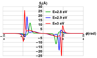
(a)

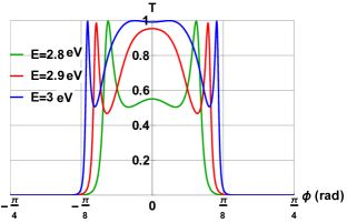
(b)

Figure 3: The GH Shift $S_{t}$ (a) and transmission probability (b) as a function of the incident angle $\phi$ for $d=10$ nm, $V=2$ eV, $d_{1}=d_{2}=d_{3}=d/3$, $V_{2}=0$ and three values of the incident energy $E$.

In Fig. 4, we show that the strength of the barrier height $V$ affects the GH shift and the transmission probability. For a better presentation, we have used an incident angle $\phi=4^{\circ}$, barrier width $d=10$ nm, the ratio $q_{2}=1/3$, and computed the transmission probabilities and GH shift for various values of the incident energy $E$. In contrast to what we saw in Fig. 2, this figure demonstrates how a negative peak precedes a positive valley in the GH shift. This behavior is observed for all energies. The values of potential at the edges of the transmission gaps are those at which the GH shift changes sign. Thus, we can conclude that the strength of the barrier height $V$ could also be used to tune the sign of the GH shift. This has a significant impact on the potential future applications of GH shift in signal processing.

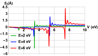
(a)

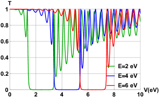
(b)

Figure 4: The GH Shift $S_{t}$ (a) and transmission probability (b) as a function of the barrier height $V$ for $\phi=4^{\circ}$, $d_{1}=d_{2}=d_{3}=d/3$, $V_{2}=0$, $d=10$ nm, and three values of the incident energy $E$.

Fig. 5 we show how GH shift and transmission probability vary as a function of the full barrier width $d$ for various values of the incident energy $E$, with  $\phi=4^{\circ}$, $V=2$ eV,$V_{2}=0$, $q_{2}=1/3$. It is obvious from Fig. 5a that the GH shift changes its sign while its magnitude increases with the incident energy $E$. We also observe that for small widths $d$ ($d<5$), the GH shift is positive, while it becomes negative for ($5<d<15$) and then oscillates afterwards. Fig. 5b shows that the transmission decays as a function of the full barrier width $d$, which exhibits oscillatory behavior as we increase $d$, similarly to what has been seen in previous work [24].

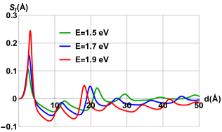
(a)

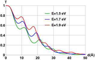
(b)

Figure 5: The GH Shift $S_{t}$ (a) and transmission probability (b) as a function of the barrier width $d$ for $\phi=4^{\circ}$, $d_{1}=d_{2}=d_{3}=d/3$, $V_{2}=0$, $V=2$ eV, and three values of the incident energy $E$.

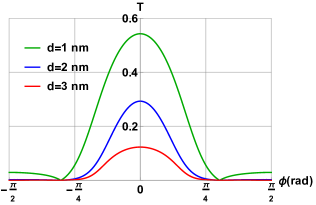
(a)

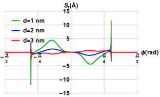
(b)

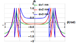
(c)

Figure 6: Transmission probability $T(\phi)$ (a), GH shifts $S_{t}(\phi)$ (b), and phase shift $\varphi_{t}(\phi)$ (c) as a function of the incident angle $\phi$ for $d_{1}=d_{2}=d_{3}=d/3$, $V=2$ eV, $V_{2}=0$, $E=1.5$ eV, and three values of the barrier width $d$.

Fig. 6 shows the transmission probability, GH shift, and phase shift dependence on the incident angle $\phi$, for $V=2$ eV, $V_{2}=0$, $q_{2}=1/3$, $E=1.5$ eV and for different values of $d=1$ (green), $2$ (blue), and $3$ (red). From Fig. 6a, we see that the maximum transmission occurs at normal incidence and increases with decreasing values of $d$, while it vanishes beyond some critical value of $\phi$. The transmission is symmetrical with respect to $\phi=0$, as you can see. From Fig. 6b, we see that both the magnitude and sign of GH shift can be altered by increasing the barrier width $d$. In Fig. 6c, we see the oscillatory and symmetric behavior of the transmission phase as a function of $\phi$. This oscillatory behavior is mostly concentrated close to $\phi=\pm\pi/4$, with a wide plateau in between, whose magnitude increases with the width of the barrier $d$.

V Conclusion

We studied the Goos-Hänchen shift for charged carriers scattering through a double barrier potential in phosphorene. Initially, we computed the eigenvalues and eigenspinors of our Hamiltonian, enabling the calculation of the corresponding transmission probability. Using these results, we determined the phase shift associated with the transmission amplitude. Subsequently, we calculated the corresponding Goos-Hänchen shift and investigated its behavior concerning various physical parameters, including the width and height of the barriers, incident energy, and incident angle. We then discussed various numerical results and highlighted their importance regarding potential applications of the Goos-Hänchen shift in optical sensors and optical waveguide switches.

As a result, we have observed that the Goos-Hänchen shift strongly depends on the incidence energy $E$. We have also pointed out that the energies at which the GH shift reaches its maximum magnitude and change sign occur at the transmission peaks just prior to and just after the gap region where the transmission vanishes. It is also noteworthy to mention that the transmission resonances are highly correlated with the oscillatory behavior of the Goos-Hänchen shift. The transmission was found to be bilaterally symmetrical with respect to incident angle $\phi$ while the GH shift was found to be an odd function of the incidence angle. However, when $\phi$ exceeds a certain critical value, the transmission vanishes due to the appearance of an evanescent wave in the barrier. We also pointed out that the barrier height $V$ can also be used to control the sign of the Goos-Hänchen shift. To sum up, our results confirm that the Goos-Hänchen shift strongly depends on the characteristics of the potential barrier and the incident angle $\phi$. Most importantly, this Goos-Hänchen shift is substantial and easily detectable, and in fact, it surpasses those observed previously in graphene, putting phosphorene at the forefront of any future potential application for optical sensors and switches.

References

- [1] H. Liu, A. T. Neal, Z. Zhu, Z. Luo, X. Xu, D. Tomnek, and P. D. Ye, ACS Nano 8, 4033 (2014).
- [2] F. Xia, H. Wang, and Y. Jia, Nat. Commun. 5, 4458 (2014).
- [3] L. Li, Y. Yu, G. J. Ye, Q. Ge, X. Ou, H. Wu, D. Feng, X. H. Chen, and Y. Zhang, Nat. Nanotechnol. 9, 372 (2014).
- [4] V. Tran, R. Soklaski, Y. Liang, and L. Yang, Phys. Rev. B 89, 235319 (2014).
- [5] K. S. Novoselov, A. K. Geim, S. V. Morozov, D. Jiang, Y. Zhang, S. V. Dubonos, I. V. Grigorieva, and A. A. Firsov, Science 306, 666 (2004).
- [6] F. Goos, H. Hänchen, Ann. Phys. 436, 333 (1947).
- [7] F. Goos, H. Hänchen, Ann. Phys. 6, 251 (1949).
- [8] K. Artmann, Ann. Phys. 2, 87 (1949).
- [9] X. Chen, J.-W. Tao, and Y. Ban, Eur. Phys. J. B 79, 203 (2011).
- [10] Y. Song, H.-C. Wu, and Y. Guo, Appl. Phys. Lett. 100, 253116 (2012).
- [11] X. Chen, P.-L. Zhao, X.-J. Lu, and L.-G. Wang, Eur. Phys. J. B 86, 223 (2013).
- [12] M. Sharma and S. J. Ghosh, J. Phys.: Condens. Matter 23. (2011) 055501.
- [13] J.-H. Huang, Z.-L. Duan, H.-Y. Ling, and W.-P. Zhang, Phys. Rev. A 77, 063608 (2008).
- [14] C. W. J. Beenakker, R. A. Sepkhanov, A. R. Akhmerov, and J. Tworzydlo, Phys. Rev. Lett. 102, 14680 (2009)4.
- [15] L. Zhao and S. F. Yelin, Phys. Rev. B 81, 115441 (2010).
- [16] Zhenhua Wu, F. Zhai, F. M. Peeters, H. Q. Xu, and Kai Chang, Phys. Rev. Lett. 106, 176802 (2011).
- [17] Parisa Majari and Gerardo G. Naumis, Physica B 668, 415238 (2023).
- [18] J. Seffadi, I. Redouani, Y. Zahidi, and A. Jellal, Solid State Commun. 351, 114777 (2022).
- [19] J. M. Pereira, Jr. and M. I. Katsnelson, Phys. Rev. B 92, 075437 (2015).
- [20] Z. S. Popović, J. M. Kurdestany, and S. Satpathy, Phys. Rev. B 92, 035135 (2015).
- [21] D. J. P. de Sousa, L. V. de Castro, D. R. da Costa, and J. M. Pereira, Phys. Rev. B 94, 235415 (2016).
- [22] Y. Zahidi, I. Redouani, and A. Jellal, Physica E 81, 259 (2016) .
- [23] L. Liu, Y.-X. Li, and J.-J. Liu, Phys. Lett. A 376, 3342 (2012).
- [24] S. De Sarkar, A. Agarwal, and K. Sengupta, J. Phys.: Condens. Matter 29, 285601 (2017).