Integrated Freeway and Arterial Traffic Control to Improve Freeway Mobility without Compromising Arterial Traffic Conditions Using Q-Learning

Abstract

Freeway and arterial transportation networks are operated individually in most cities nowadays. The lack of coordination between the two increases the severity of traffic congestion when they are heavily loaded. To address the issue, we propose an integrated traffic control strategy that coordinates freeway traffic control (variable speed limit control, lane change recommendations, ramp metering) and arterial signal timing using Q-learning. The agent is trained offline in a single-section road network first, and then implemented online in a large simulation network with real-world traffic demands. The online data are collected to further improve the agent’s performance via continuous learning. We observe significant reductions in freeway travel time and number of stops and a slight increase in on-ramp queue lengths by implementing the proposed approach in scenarios with traffic congestion. Meanwhile, the queue lengths of adjacent arterial intersections are maintained at the same level. The benefits of the coordination mechanism is verified by comparing the proposed approach with an uncoordinated Q-learning algorithm and a decentralized feedback control strategy.

I Introduction

Demand for freeway and arterial travel grows in a fast pace as the population increases in metropolitan areas worldwide, leading to traffic congestion and delays at sensitive parts of road networks such as ramps and intersections. Research efforts on freeway [1, 2, 3] and arterial traffic management [4, 5, 6] as separate entities have both achieved certain levels of success in terms of reducing travel time, collision risks and emission rates. However, the integration of freeway and arterial traffic control has been rarely explored due to the difficulty of modeling two completely different traffic patterns and high complexity of the road network. In practice, the coordinated operation of freeways and adjacent arterials is hindered by the fact that the two facilities are typically managed by two separate authorities with different objectives and limited communications [7]. Despite the above mentioned restrictions, a few studies have verified the effectiveness of coordinating ramp metering (RM) with adjacent arterial traffic signals [8, 9, 10], which reveals the great potential of coordinating freeway and arterial (CFA) traffic control on improving the operation efficiency.

Popular freeway traffic control techniques include variable speed limit (VSL) control, lane change (LC) control and ramp metering (RM). During the last few decades many research efforts on one or a combination of the above three methods have been proposed to alleviate congestion at freeway bottlenecks. The VSL controller regulates the traffic flow via variable speed commands in order to protect the bottleneck flow to stay at its maximum possible value and reduce the effect of capacity drop [11]. VSL control techniques designed using macroscopic models failed to take into account the forced lane changes at the bottleneck leading to capacity drop which VSL control cannot effectively handle [12, 13, 14]. To address this issue, LC recommendations are used at the upstream area of the bottleneck to guide the vehicles onto open lanes in advance and reduce the forced lane changes and the consequential capacity drop [15]. Ramp metering controls the inflow of traffic to the freeway lanes by adjusting the traffic signal timing at each on-ramp entrance. Despite the promising effect of RM in theory [16, 1], the on-ramp space is frequently saturated during peak hours, which forces RM to switch off and offers no benefits when it is needed the most. Although alternative solutions which consider the balance of freeway occupancy and on-ramp queue length have been proposed [17, 18], the improvement is still limited when both freeway traffic loads and on-ramp demands are high.

The above facts motivate us to examine a more intuitive solution by connecting the ramps with adjacent arterial road networks and collecting arterial traffic states to assist the management of on-ramp demands, as pointed out by a few CFA studies [8, 9, 10]. We extend these efforts by integrating all the previous mentioned freeway traffic regulation techniques (VSL, LC, RM) with arterial traffic signal control (TSC) to mitigate congestion for a complex road network involving freeway and adjacent arterial intersections under different demand levels and incident scenarios. To facilitate the coordination between different control components, we adopt a Q-learning (QL) framework where a common reward function is defined for VSL, LC and RM actions and adjacent arterial signal plans are incorporated into the state set.

The contributions of this paper are summarized as follows:

1. We develop an integrated freeway and arterial traffic control strategy that coordinates VSL, LC, RM and arterial signal plans using QL algorithm. The QL agent determines the VSL, LC and RM actions based on a common reward function that contains the travel time, the on-ramp queue and the traffic density. The state set of the QL agent involves the signal plan and estimated demands of the adjacent arterial intersection in order to improve the control performance.

2. We propose a traffic-responsive signal control strategy that computes the arterial signal plan via a simulation-based cycle length model and estimated demands of all intersection approaches.

3. The numerical simulation results indicate that the proposed coordination mechanism improves the freeway traffic mobility without compromising arterial traffic conditions compared with uncoordinated control strategies in congested scenarios. The coordination is less effective when the network is not congested.

The rest of the paper is organized as follows: section II reviews relevant literature. Section III presents the integrated freeway and arterial traffic control strategy. Section IV verifies the effectiveness of the proposed approach via microscopic simulations. Section V concludes the paper.

II Literature Review

The proposed integrated control consists of variable speed limit (VSL) control, lane change (LC) recommendations, ramp metering (RM) and arterial traffic signal control (TSC). We first review relevant research efforts for each component separately, and then discuss the frameworks to coordinate these components to achieve higher performance.

Early VSL control designs aimed at stabilizing mainstream traffic flows and minimizing speed variations with reactive rule-based logic [19, 20]. The reactive nature of these approaches introduces time lags between VSL actions and traffic conditions, and thus, leads to limited performance in terms of travel time and energy consumption. In contrast, many recent developed VSL algorithms compute the speed commands by solving an optimization problem at each time step based on predictions of future traffic states using model predictive control (MPC) techniques [21, 22, 23, 24]. The objective function to be optimized typically consists of total travel time, safety measurements, emission rates and fuel consumption. Although MPC-based approaches improve the control performance by eliminating time lags of VSL command activation compared to reactive rule-based approaches, they do not guarantee the stability of vehicle densities and require substantial computational efforts when applied to large-scale road networks. Another well-known alternative is to design a feedback law to compute appropriate speed limits using current and past traffic states [25, 26, 27], which consumes much less computational efforts than MPC-based approaches. In addition, feedback-based VSL controller guarantees the convergence of mainstream traffic flows and densities analytically [28]. However, feedback-based approaches rely on accurate measurements of traffic states to generate effective control actions. A small deviation from the true value on sensitive variables, vehicle densities for example, may produce unsatisfactory closed-loop behaviors [29, 30]. Some reinforcement learning (RL)-based VSL control schemes have been proposed recently as a promising approach to guarantee the optimality via trial and error [31, 32]. Although the learning process of RL agents can be very time-consuming, the field implementation is fast, and thus, applicable for large-scale road networks.

Lane change control is considered as an effective approach to improve lane-drop bottleneck throughput [33, 34]. However, in most integrated control schemes [15, 35, 11], the LC control is designed as rudimentary rules and produces less benefits compared with other controllers such as the VSL. Recently, the LC control has been extended to on-ramp merging bottlenecks using much more mature feedback laws [36, 37]. Both studies [36, 37] assume a connected vehicle environment and balance the lane usage by assigning proper lateral flows.

Since ramps connect freeways with arterial streets, an appropriate ramp metering design should balance the traffic loads of both regions. Some isolated RM algorithms were first proposed in 1990s [38, 39], including the famous ALINEA [16], which takes freeway occupancy as input and computes the metering rate in a local feedback manner. The classic ALINEA does not consider the potential spillback of on-ramp queues under high traffic demands. Therefore, it was modified in [17] to avoid the overextension of on-ramp queues by including both the mainstream occupancy and the queue length in the feedback loop. Due to the fact that ramp flows are also affected by the mainstream traffic, coordinated RM algorithms that take into account both local and system-wide traffic conditions typically outperform isolated RM algorithms. In [40], Paesani et al. proposed a system-wide adaptive RM algorithm to compute the metering rates based on estimated future traffic states with linear regression. The lack of accurate real time data makes such methods deviate considerably from the theoretical best performance. In [41], another extension of ALINEA was made by connecting all the on-ramps via a central controller and dynamically distribute the ramp demands. When one on-ramp queue reaches the threshold, the central controller increases the throughput of this particular on-ramp while decreases the throughput of other on-ramps. In [42], a similar two-level structure was embedded into the RM algorithm. The upper level controller determines the optimal total inflow using MPC framework, and the lower level controller distributes the computed total inflow to each on-ramp. Although improvement can be observed by coordinating each RM controller within the network, the control performance is still limited when heavy traffic exists in the mainstream, as RM only affects the vehicle density closely downstream of the on-ramp.

Traffic signal control is considered as the most important and effective method to manage arterial traffic. Existing TSC strategies can be divided into two categories: fixed-time TSC and traffic-responsive TSC. Fixed-time TSC switches between predetermined signal programs according to the time of the day, and thus, suitable for stable, unsaturated traffic conditions. In [43, 44], F. V. Webster designed a signal timing model to minimize the travel delay, and developed the basis for modern fixed-time TSC design. Two of the most widely implemented and extended fixed-time TSC strategies are MAXBAND [45] and TRANSYT [46]. MAXBAND coordinates traffic signals along an arterial with the same cycle length and proper offsets so that vehicles can travel without stopping, which formulates a progression band with a uniform bandwidth to be maximized. Representative extensions of MAXBAND include assigning multiple bandwidths for different road segments [47], incorporating route guidance [48], or speed advisory [4]. TRANSYT takes historical traffic data of the road network as input, and then determines the optimal signal control with a heuristic ”hill climbing” algorithm. The major limitation of fixed-time TSC is that it cannot handle highly saturated traffic conditions or incident scenarios, which prompts the study of real-time traffic-responsive TSC. In [49], a traffic-responsive version of TRANSYT - SCOOT, was developed to adjust signal cycles, splits and offsets with newly-measured traffic flows and occupancy. In [50], a real-time hierarchical optimized distributed effective system (RHODES) was proposed with two main operation processes. The first process uses sensor data to estimate future traffic flows within the network. The second process selects the optimal phasing time with dynamic programming (DP) and decision trees. Despite their satisfactory performance in numerous field tests, most traffic-responsive TSC systems rely on accurate real-time traffic data and a powerful central machine to solve optimization algorithms whose complexity grows exponentially with the size of the problem leading to costly implementation with restrictions on the size of arterial networks.

To coordinate different control components for mixed freeway and arterial road networks, the most intuitive method is to formulate an optimization problem so that all the controllers dedicate to the same objective function [8, 1, 9]. In [8, 9], separate models are developed to characterize the freeway part and the arterial regions, and then MPC-based control schemes are proposed to minimize the total time spent/delay. Both studies have verified the performance improvement by using a centralized control over the mixed road network, but the considered traffic regulation techniques only involve RM and TSC. Moreover, MPC-based algorithms produce tremendous computational cost for large-scale road networks. Scalable alternatives have been proposed based on shock wave theory, feedback control or logic rules [51, 52, 3]. A common drawback of these algorithms is the lack of coordination between different control components. In [53], an RL framework is adopted to integrate VSL and RM for freeway traffic control, which guarantees the optimality and is efficient enough for large networks. The framework can be potentially extended to involve LC control and TSC as well.

III Methodology

In this section, we propose an integrated control strategy to regulate the traffic in a road network consisting of both freeway and the adjacent arterial region (depicted in Fig. 1) with the purpose of reducing the vehicle travel time and the emission rates, meanwhile maintaining the queue lengths of on-ramps and intersections to a reasonable level under all traffic conditions and input demands. Traffic data and control inputs are shared between the two systems to enhance the control performance. Note that all the freeway ramps are connected with arterial roads. Some connections are omitted in Fig. 1 due to limited drawing space. More details of the road network configuration will be presented later in the section. The notations used hereafter are summarized in Table I.

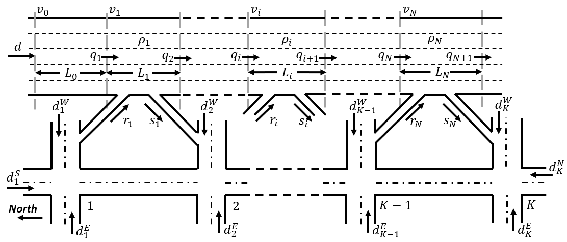
Figure 1: Road network consisting of a freeway segment and adjacent arterials.

TABLE I: Definition of Variables and Model Parameters

Symbol	Definition	Unit
$d$	the freeway vehicle input	veh/h
$d^{E}_{k}$	the vehicle input of arterial intersection $k$ with the direction specified by the superscript ($E$ stands for Eastbound)	veh/h
$C$	the capacity of each freeway section	veh/h
$C_{b}$	the bottleneck capacity	veh/h
$q_{i}$	the mainstream inflow of freeway section $i$	veh/h
$q_{i+1}$	the mainstream outflow of freeway section $i$	veh/h
$r_{i}$	the on-ramp inflow of freeway section $i$	veh/h
$s_{i}$	the off-ramp outflow of freeway section $i$	veh/h
$v_{i}$	the speed limit command of freeway section $i$	km/h
$v_{f}$	the free flow speed	km/h
$w$	the back propagation speed	km/h
$\tilde{w}$	the rate that the outflow $q_{i+1}$ decreases with density $\rho_{i}$, when $\rho_{i}\geq\rho_{c}$ [54]	km/h
$\rho_{c}$	the critical density of the freeway section, at which $v_{f}\rho_{c}=w(\rho^{j}-\rho_{c})=\tilde{w}(\tilde{\rho}^{j}-\rho_{c})=C$	veh/km
$\rho^{j}$	the jam density at which the inflow $q_{i}$ decreases to 0 with rate $w$	veh/km
$\tilde{\rho}^{j}$	the jam density at which the outflow $q_{i+1}$ decreases to 0 with rate $\tilde{w}$	veh/km
$\rho_{i}$	the density of freeway section $i$	veh/km
$L_{i}$	the length of freeway section $i$	km
$\epsilon_{0}$	the capacity drop factor, where $\epsilon_{0}\in(0,1)$	unitless

III-A Reinforcement Learning

The coordination between different components is the key to improving the performance of the proposed integrated control strategy. In typical rule-based or feedback-based control algorithms [52, 3, 29], each controller attempts to achieve its own goal without coordination. In optimization-based control algorithms [8, 1, 9], the coordination is addressed as multiple controllers attempting to optimize the same objective. However, the formulation of the optimization problem is tedious for the considered road network due to its high complexity which does not scale up as the network grows in size.

Reinforcement learning (RL) is a promising alternative approach that enhances the coordination between different controllers and requires less computational effort than optimization-based algorithms in terms of field implementation [53]. The RL agent interacts with the environment and attempts to maximize the cumulative reward by trial and error in discrete time steps, which can be formulated as a Markov decision process (MDP). The MDP contains a set of environment states and a set of control actions. Let $P_{a}(x,x^{\prime})$ denote the probability of transition from state $x$ to another state $x^{\prime}$ by taking action $a$, and let $R_{a}(x,x^{\prime})$ denote the reward received from the environment by making the transition from $x$ to $x^{\prime}$ through action $a$. For each state-action pair $x$ and $a$, the expected discounted reward received by taking action $a$ in state $x$ is expressed as a Q-value function $Q(x,a)$. To solve the MDP problem, we need to find a policy $\pi$ that defines the action that leads to the maximal Q-value in each state, i.e.

$$\pi^{*}(x)=\operatorname*{arg\,max}_{a}Q(x,a)$$ (1)

where $Q(x,a)$ can be expressed as

$$Q(x,a)=\sum_{x^{\prime}}P_{a}(x,x^{\prime})(R_{a}(x,x^{\prime})+\gamma\max_{a^{\prime}}Q(x^{\prime},a^{\prime}))$$ (2)

in which $\gamma\in[0,1)$ is the discount factor.

The solution of (1) can be calculated using dynamic programming if the transition probability and the reward function are known. However, in the context of traffic flow control, neither the transition probability nor the reward function can be expressed explicitly. Therefore, we have to apply model-free solution techniques such as the Q-learning (QL) algorithm [55] to learn the optimal policy. The QL agent learns the Q-value function by taking actions and observing rewards for each state. Assume that the state transition from $x$ to $x^{\prime}$ takes place by executing action $a$ and the reward $R$ is observed, then the Q-value can be updated as follows

$$Q(x,a)=Q(x,a)+\eta(R+\gamma\max_{a^{\prime}}Q(x^{\prime},a^{\prime})-Q(x,a))$$ (3)

where $\eta\in(0,1]$ is the learning rate.

III-B Freeway Traffic Model

To demonstrate the implementation of the QL algorithm in terms of freeway traffic control, we first introduce the Cell Transmission Model (CTM), which is adopted to describe the traffic behaviors of the freeway segment because of its high computational efficiency and reasonable accuracy [56, 57, 58, 28] compared with higher-order models [59, 60]. Under the framework of CTM, the selected freeway segment is divided into $N$ sections/cells and indexed from 1 to $N$ along the traffic flow direction, as shown in Fig. 1. Each section/cell is characterized by the vehicle density, mainstream inflow, mainstream outflow, on-ramp inflow, off-ramp outflow and section length, denoted as $\rho_{i},q_{i},q_{i+1},r_{i},s_{i},L_{i}$ respectively, where $i=1,2,...,N$. Without loss of generality, it is assumed that an incident occurs and creates a bottleneck at section $M$ ($1<M\leq N$), as shown in Fig. 2.

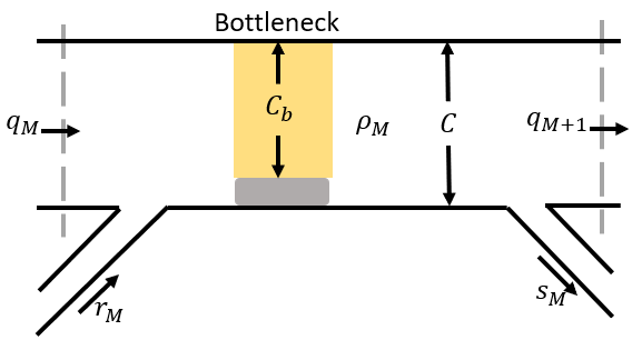
Figure 2: Freeway bottleneck in an arbitrary CTM section.

Although the original CTM can reproduce the traffic dynamics in normal circumstances, it does not capture the capacity drop phenomenon and bounded acceleration effects produced by forced lane change maneuvers at freeway bottlenecks or ramp merging areas [61, 58]. To address the issue and improve the consistency with microscopic observations, a modified multi-section CTM that accommodates the effect of both capacity drop and bounded acceleration is considered [28]. Accordingly, the following equations describe the evolution of the vehicle density $\rho_{i}$ in each section:

$$\dot{\rho}_{i}=\frac{1}{L_{i}}\left(q_{i}-q_{i+1}+r_{i}-s_{i}\right),\quad\text{for}\ i=1,...,N,$$ (4)

where

$$q_{1} =\min\big{\{}d,C,w(\rho^{j}-\rho_{1})\big{\}},$$ (5)

$$q_{i} =\min\big{\{}v_{f}\rho_{i-1},\tilde{w}(\tilde{\rho}^{j}-\rho_{i-1}),C,w(\rho^{j}-\rho_{i})\big{\}},$$

$$\qquad\quad\ \ \text{for}\ i=2,...,M-1,M+2,...,N,$$

$$q_{M} =\min\big{\{}v_{f}\rho_{M-1},\tilde{w}(\tilde{\rho}^{j}-\rho_{M-1}),(1-\epsilon(\rho_{M}))C_{b},$$

$$\qquad\quad\ \ w(\rho^{j}-\rho_{M})\big{\}},$$

$$q_{M+1} =\min\big{\{}v_{f}\rho_{M},\tilde{w}(\tilde{\rho}^{j}-\rho_{M}),(1-\epsilon(\rho_{M}))C_{b},$$

$$\qquad\quad\ \ w(\rho^{j}-\rho_{M+1})\big{\}},$$

$$q_{N+1} =\min\big{\{}v_{f}\rho_{N},C,\tilde{w}(\tilde{\rho}^{j}-\rho_{N})\big{\}},$$

and

$$\epsilon(\rho_{M})=\left\{\begin{aligned} &\epsilon_{0}&&\text{if }C_{b}<C\text{ and }\rho_{M}>\frac{C_{b}}{v_{f}}\\ &0&&\text{otherwise}\end{aligned},\right.$$

III-C Q-Learning Based Freeway Traffic Control

Based on the CTM presented above, this section aims to develop a coordinated variable speed limit (VSL), lane change (LC) and ramp metering (RM) controller to smooth on-ramp merging, reduce freeway travel time, and alleviate the congestion produced by a lane-drop bottleneck in arbitrary section $M$ ($1<M\leq N$). The controller determines the optimal policy using the QL algorithm for each CTM section, as depicted in Fig. 3. The adjacent arterial traffic states and signal plan are also taken into account to enhance the coordination between the freeway and arterials. The flowchart of the proposed control strategy is depicted in Fig. 4.

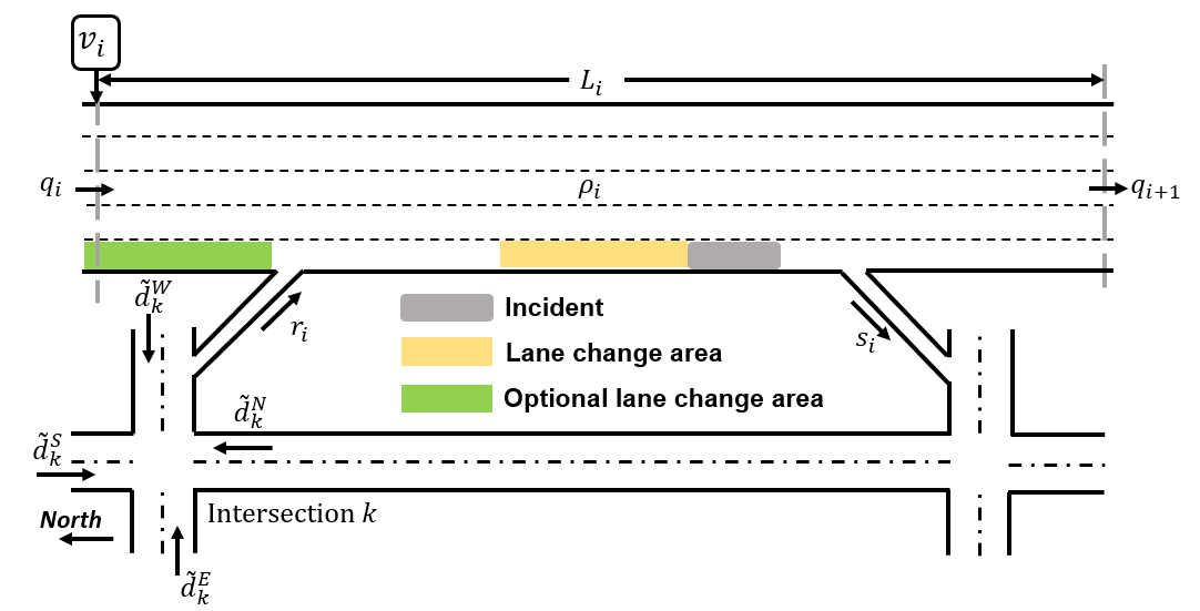
Figure 3: Road network of a single freeway CTM section with adjacent arterials.

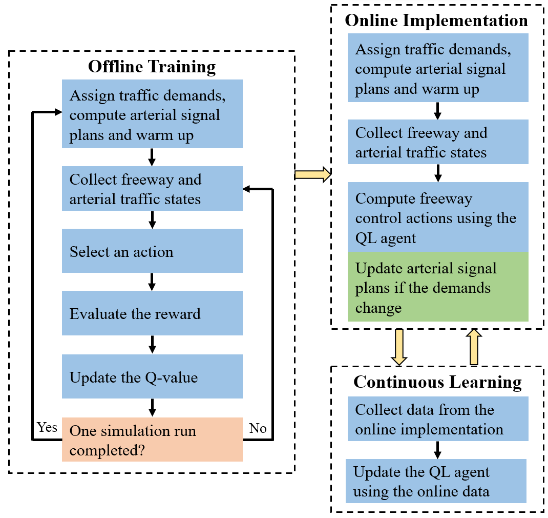
Figure 4: Flowchart of the proposed QL-based control strategy.

As illustrated in Fig. 4, we first perform offline training over the small road network depicted in Fig. 3. During the training process, we explore as many state-action pairs as possible by running multiple simulations for each traffic demand level. Each simulation run lasts for 30 min (60 time steps) with a warm-up of 5 min. After the warm-up, there is a 20% chance that an incident takes place and block the side lane. Once the offline training is completed, we implement the trained QL agent in a large simulation road network with real-world traffic demands from PeMS. Then we collect data from the online implementation to assist the continuous learning of the QL agent. The cycle of online implementation and continuous learning can be repeated multiple times to improve the control performance. The detailed configurations of the online implementation is demonstrated in section IV-A. The arterial signal control scheme is introduced in section III-D.

To formulate the proposed freeway control problem as a MDP, we introduce the definition of environment states, action space, reward function and some other important variables and parameters in the rest of the section.

III-C1 State Description

The environment states for the proposed integrated control involve measured and estimated traffic data of the freeway CTM section $i$ and the adjacent arterial intersection $k$, illustrated graphically in Fig. 3 and listed as follows

• Vehicle density: $\rho_{i}$.

• Inflow from the upstream CTM section: $q_{i}$.

• Outflow toward the downstream CTM section: $q_{i+1}$.

• On-ramp traffic flow: $r_{i}$.

• Off-ramp traffic flow: $s_{i}$.

• On-ramp queue length: $w_{i}$.

• The lane closure (incident) flag: $n_{c}\in\{0,1\}$.

• The dominant signal phase of intersection $k$ in the next control cycle: $n_{p}\in\{1,2,3,4,5\}$.

• Estimated demand of each approach of intersection $k$: $\tilde{d}^{E}_{k}$, $\tilde{d}^{S}_{k}$, $\tilde{d}^{W}_{k}$, $\tilde{d}^{N}_{k}$, where the superscript denotes the direction of the approach. The estimation process will be introduced in section III-D.

III-C2 Action Space

The action space of the variable speed limit control $A(v_{i})$ contains a set of speed limit values that can be applied to each freeway CTM section. Considering the feasibility in the real world, we set the speed limit to be a multiple of 10 km/h with a minimum value of 60 km/h and a maximum value of 100 km/h. The speed limit value can be increased or decreased by at most 10 km/h to ensure safety. Therefore,

$$\begin{split}A(v_{i}(t))&=\{\max\{60,v_{i}(t-T)-10\},\\ &v_{i}(t-T),\min\{100,v_{i}(t-T)+10\}\}\end{split}$$ (6)

where $T$ is the control cycle.

The ramp metering agent has a fixed green phase duration of 3 s and adjusts the red phase duration according to the traffic states. The set of available red phase durations is $\{0,0.5,1,1.5,2,3,4,6\}$ in seconds, which corresponds to the following set of on-ramp flow rates $\{1800,1029,900,800,720,600,514,400\}$ in vehicles per hour.

To mitigate the capacity drop triggered by forced lane change maneuvers and increase the throughput at the bottleneck, we provide lane change (LC) recommendations to vehicles moving in the closed lane(s) before approaching the bottleneck, as depicted in Fig. 3. We also provide LC recommendations on the upstream area of on-ramp merging if it improves the overall performance, for which the LC agent needs to make a decision. Therefore, the action space of the LC control is binary, i.e. whether or not to activate the LC recommendations on the upstream area of on-ramp merging.

III-C3 Reward Function

The objective of the proposed freeway control strategy is to reduce vehicle travel time while maintaining on-ramp queues at reasonable levels. The average travel time can be computed as

$$T_{t}=\frac{1}{N_{v}}\sum_{j=1}^{N_{v}}(t_{j,out}-t_{j,in})$$ (7)

where $N_{v}$ is the number of vehicles passing through the CTM section during the current control cycle, $t_{j,in}$ and $t_{j,out}$ is the time vehicle $j$ enters and exits the section respectively.

A reasonable reward function must be negatively correlated with the average travel time $T_{t}$ and the on-ramp queue length $w_{i}$. To avoid on-ramp queue overspill, we want the reward $R<0$ when $w_{i}$ exceeds the reference value $w_{i}^{r}$. Moreover, we want the vehicle density $\rho_{i}$ to be close to the desired density $\rho^{*}$, and thus, $R$ should be negatively correlated with the distance between $\rho_{i}$ and $\rho^{*}$. Considering the above requirements, the reward function $R$ is defined as

$$R=(1-\frac{w_{i}}{w_{i}^{r}})\frac{L_{i}}{T_{t}v_{f}}-(\frac{\rho_{i}}{\rho^{*}}-1)^{2}$$ (8)

III-C4 Other Variables and Parameters

As mentioned previously, the reward function (8) encourages the density of each CTM section to converge to a predefined value, denoted as $\rho^{*}$. In the ideal case, a trivial choice is to let $\rho^{*}=\min\{d,C_{b}\}/v_{f}$, which corresponds to the highest possible flow-rate through the bottleneck. However, a small disturbance may drive the density towards the capacity-drop region, which introduces unwanted oscillatory behavior of the closed-loop system and negatively impacts convergence to desired equilibrium states [30]. To avoid the capacity drop triggered by the disturbance, we multiply $C_{b}$ with a factor that is slightly less than $1$, and thus, $\rho^{*}=\min\{d,0.95C_{b}\}/v_{f}$.

The proposed QL algorithm does not cover the control of the upstream part of the freeway segment, which involves two crucial variables - the value and the location of the most upstream VSL sign, denoted as $v_{0}$ and $L_{0}$ in Fig. 1. According to [11], the inflow $q_{1}$ is regulated by $v_{0}$ so that $q_{1}$ is less than or equal to the bottleneck throughput. The fundamental diagram (FD) indicates that the maximum possible flow produced by $v_{0}$ is $\frac{v_{0}w\rho^{j}}{v_{0}+w}$. Combining the FD relationship with (5), we have

$$v_{0}=\left\{\begin{aligned} &\frac{wC_{b}}{w\rho^{j}-C_{b}}&&\text{if }d>C_{b}\ \&\ 0\leq\rho_{M}\leq\frac{C_{b}}{v_{f}},\\ &\frac{w(1-\epsilon_{0})C_{b}}{w\rho^{j}-(1-\epsilon_{0})C_{b}}&&\text{if }d\geq(1-\epsilon_{0})C_{b}\ \&\ \rho_{M}>\frac{C_{b}}{v_{f}},\\ &v_{f}&&\text{otherwise}\end{aligned}\right.$$ (9)

On the other hand, we set $L_{0}$ to be slightly greater than the lower bound proposed in [11], i.e.

$$L_{0}>\frac{v_{f}\bar{\rho}(t_{0})-(1-\epsilon_{0})C_{b})v_{0}L_{b}}{((1-\epsilon_{0})C_{b}-v_{0}\rho_{0}(t_{0}))v_{f}}$$ (10)

where $\bar{\rho}$ is the average density from section 1 to $M$; $L_{b}$ is the distance from the beginning of section 1 to the lane-drop bottleneck; $t_{0}$ is the time the incident takes place.

In LC control, the distance of the LC area, denoted as $d_{LC}$, is a crucial control variable that needs to be determined properly. $d_{LC}$ must be longer than the minimum distance required for vehicles to complete LC maneuvers safely, but overextending $d_{LC}$ may lead to the underutilization of the road capacity. In this paper, $d_{LC}$ takes an empirical value of 800 m for both on-ramp merging and lane-closure bottlenecks [15].

The learning rate $\eta$ is one of the most important QL parameters. A common strategy is to set a decreasing $\eta$ over the training process to ensure reasonable efficiency and the convergence of the Q value. Note that letting $\eta$ decrease as a function of time does not work well because different states and actions are visited at different stages of the learning process. Instead, we assign a specific $\eta$ to each state-action pair and reduce its value every time the state-action pair has been visited [32]. Therefore,

$$\eta(x,a)=\biggr{[}\frac{1}{1+n(x,a)(1-\gamma)}\biggr{]}^{0.8}$$ (11)

where $n(x,a)$ is the number of times the state-action pair $(x,a)$ has been visited and $\gamma$ is the discount factor.

To balance exploration and exploitation during the learning process, we implement an adaptive greedy policy where a random action is selected with probability $\delta$ and the best-known action is selected with probability $1-\delta$. Similar to the learning rate equation above, $\delta$ is designed as a function of the number of prior visits to each state [53], i.e.

$$\delta(x)=\max\biggl{\{}0.05,\frac{1}{1+\frac{1}{4N_{a}(x)}\sum_{n=1}^{a}n(x)}\biggl{\}}$$ (12)

where $N_{a}(x)$ is the number of available actions at the state $x$, $n(x)$ is the number of prior visits of the state $x$. The adopted greedy policy encourages the agent to take random actions (exploration) when a state has not been visited, and becomes more likely to take the best-known action (exploitation) as the number of visits increases. The probability of exploration eventually converges to a minimum value of $0.05$.

III-D Arterial Traffic Signal Control

The arterial road network under consideration contains $K$ homogeneous signalized intersections indexed from 1 to K in the freeway traffic flow direction, as depicted in Fig. 1. The on-ramp entrances and off-ramp exits lie on the East side of each intersection. There are $2(K+1)$ entrances plus $N$ off-ramps that generate traffic flow into the arterial road network. At this stage, we assume traffic signal control (TSC) is the only method to regulate arterial traffic flows. Fixed-time TSC strategies cannot fit various input levels and traffic conditions as mentioned in section II. Therefore, we propose a traffic-responsive scheme to determine the signal plan that minimizes the travel time, the fuel consumption and the emissions for each intersection based on the observation of input demands and turning ratios.

III-D1 Cycle Length Model

The first step of the proposed TSC scheme is to find a cycle length model that fits the arterial traffic conditions. The pioneer research on signal cycle optimization was conducted by F. V. Webster [43, 44], who developed a formula to compute the signal cycle that minimizes travel delays while considering the uncertainties of traffic models as follows:

$$T_{c}=\frac{1.5T_{l}+5}{1-Y}$$ (13)

where $T_{c}$ is the signal cycle and $T_{l}$ is the lost time per cycle. The lost time is defined as the time during which no vehicles are able to pass through an intersection due to the transition between a green phase and a red phase. $Y\in[0,1)$ is the sum of flow ratios of each phase group, which indicates the degree of saturation of an intersection. The flow ratio is defined as the actual traffic flow divided by the saturation flow. The saturation flow is set to be 1800 veh/h/lane in this paper. Extensions based on the Webster model have been made over the years to optimize different objective functions such as fuel consumption, emissions and the number of vehicle stops [62, 63, 64]. In this paper, we adopt the modified Webster model proposed by Calle-Laguna et al. [64]:

$$T_{c}=\alpha_{1}\ln(\frac{T_{l}}{1-Y})+\alpha_{2}$$ (14)

where $\alpha_{1}$ and $\alpha_{2}$ are determined by solving a linear regression problem on the data collected from microscopic simulations over an isolated intersection. The detailed configuration of the isolated intersection is presented in Fig. 5. Each intersection is four lanes wide (left, right, and a double through) with a length of 100 m. The arterial road connected to the intersection is two lanes wide and lasts for 1 km on each direction in order to accommodate the long queue under high demands. The default signal plan involves five phases as shown in Fig. 6. Since only medium and high traffic demands are considered, all signal plans must have a separate left-turn phase to enhance the mobility and safety of the intersection operation [65].

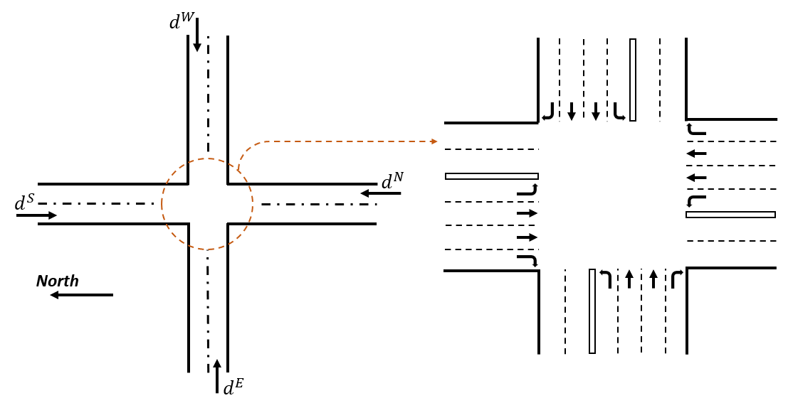
Figure 5: The configuration of an isolated intersection.

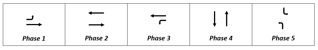
Figure 6: The phasing scheme of the default signal plan.

The commercial microscopic simulator PTV VISSIM 10 is used to generate the data for estimating the model parameters $\alpha_{1}$ and $\alpha_{2}$ in (14). For each demand, we evaluate multiple cycles using the following performance index function [62]:

$$P=\gamma_{1}\frac{T_{t}}{T_{t,0}}+\gamma_{2}\frac{F}{F_{0}}+\gamma_{3}\frac{E}{E_{0}}$$ (15)

where $T_{t}$ is the average travel time, $F$ is the average fuel consumption, $E$ is the average emission rates of CO₂, and $\gamma_{1},\gamma_{2},\gamma_{3}$ are the corresponding weights. $F$ and $E$ are computed using the EPA MOVES model [66]. $T_{t,0},F_{0},E_{0}$ are the base-case results obtained from the scenario where the signal cycle $T_{c}=60$ s. According to [62], we set $\gamma_{1}=0.4,\gamma_{2}=\gamma_{3}=0.3$.

After iterating the data collection process for all input levels twice, we plot the data points with the lowest performance index and perform the linear regression in Fig. 7. As a result, $\alpha_{1}=136.8,\alpha_{2}=-357.7$.

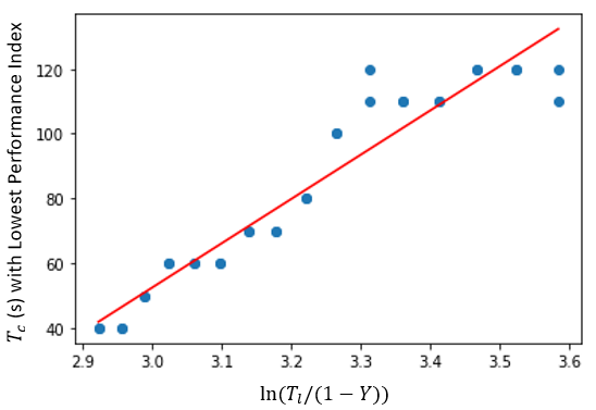
Figure 7: Data points and the linear regression curve to determine the cycle length model for the considered intersection.

III-D2 Demand and Flow Ratio Estimation

To determine signal plans using the obtained cycle length model, we estimate the demands of each intersection as follows:

$$\tilde{d}_{k}^{W} =d_{k}^{W}+\bar{s}_{i}$$ (16)

$$\tilde{d}_{k}^{E} =d_{k}^{E}$$

$$\tilde{d}_{k}^{S} =\left\{\begin{aligned} &d_{1}^{S}&&\text{if }k=1,\\ &y_{k-1}^{W,l}\tilde{d}_{k-1}^{W}+y_{k-1}^{E,r}\tilde{d}_{k-1}^{E}+y_{k-1}^{S,t}\tilde{d}_{k-1}^{S}&&\text{otherwise }\\ \end{aligned}\right.$$

$$\tilde{d}_{k}^{N} =\left\{\begin{aligned} &d_{K}^{N}&&\text{if }k=K,\\ &y_{k+1}^{W,r}\tilde{d}_{k+1}^{W}+y_{k+1}^{E,l}\tilde{d}_{k+1}^{E}+y_{k+1}^{N,t}\tilde{d}_{k+1}^{N}&&\text{otherwise }\\ \end{aligned}\right.$$

where $\tilde{d}_{k}^{W}$ is the estimated demand of the Westbound approach at intersection $k$, $d_{k}^{W}$ is the actual Westbound vehicle input of intersection $k$, $\bar{s}_{i}$ is the historical average off-ramp flow rate of CTM section $i$ from PeMS ($\bar{s}_{i}=0$ if the off-ramp does not exist), $y_{k}^{W,l}$ is the left-turn ratio of the Westbound approach at intersection $k$. The superscript denotes the traffic flow direction in the following manner: $E$ - Eastbound, $W$ - Westbound, $N$ - Northbound, $S$ - Southbound, $l$ - left-turn, $r$ - right-turn, $t$ - through. We assume CTM section $i$ is associated with intersection $k$, all vehicle inputs are known and all links within the arterial network are unsaturated. The estimation process of turning ratios will be illustrated in section IV-A.

Then we calculate the flow ratio of each phase group with respect to the phase scheme presented in Fig. 6 and sum them up to obtain $Y$:

$$Y_{1} =\frac{\tilde{d}^{S}}{q_{s}^{S}}$$ (17)

$$Y_{2} =\frac{(y^{S,r}+y^{S,t})\tilde{d}^{S}}{q_{s}^{S}}+\frac{(y^{N,r}+y^{N,t})\tilde{d}^{N}}{q_{s}^{N}}$$

$$Y_{3} =\frac{\tilde{d}^{N}}{q_{s}^{N}}$$

$$Y_{4} =\frac{(y^{W,r}+y^{W,t})\tilde{d}^{W}}{q_{s}^{W}}+\frac{(y^{E,r}+y^{E,t})\tilde{d}^{E}}{q_{s}^{E}}$$

$$Y_{5} =\frac{y^{W,l}\tilde{d}^{W}}{q_{s}^{W}}+\frac{y^{E,l}\tilde{d}^{E}}{q_{s}^{E}}$$

$$Y =Y_{1}+Y_{2}+Y_{3}+Y_{4}+Y_{5}$$

where $q_{s}$ is the saturation flow of the approach whose direction is specified by the superscript. In this paper, $q_{s}=7200$ veh/h for all directions at each intersection. Since (17) applies to all intersections in the road network, the index of the intersection is omitted for the sake of simplicity.

III-D3 Cycle Length and Split Computation

We compute the signal cycle $T_{c}$ for each intersection using (14) with the following feasibility constraints:

• 40 s $\leq T_{c}\leq$ 180 s.

• $T_{c}$ is rounded to be a multiple of 20.

Once $T_{c}$ is determined, we can allocate the green light time for each phase according to the flow ratios found in (17):

$$T_{g,j}=\frac{(T_{c}-T_{l})Y_{j}}{Y},\quad\text{for}\ j=1,2,3,4,5,$$ (18)

where $T_{g,j}$ denotes the green light time of phase $j$ per cycle, and the lost time $T_{l}=16$ s.

To minimize travel delays and improve the traffic mobility, it is recommended to unify the cycle length for closely spaced traffic signal and use proper offsets to create a progression band (green wave) for vehicle platoons on the main street [65]. However, the intersections in our simulation network are relatively far apart with a minimum distance of 600 m and 1500 m on average. Besides, the longitudinal traffic is not significantly larger than the lateral traffic at each intersection. Therefore, the offset optimization is not considered in this paper. The offset of each signal is simply set to 0 s.

IV Numerical Simulations

IV-A Simulation Network and Parameters

The proposed control methodologies are simulated using a microscopic traffic simulator based on the commercial software PTV Vissim 10. The road network in Fig. 8 contains a 16-km segment of I-710 freeway and the adjacent arterial region in Los Angeles, California, United States. The freeway segment is divided into 6 CTM sections and one upstream VSL zone. Each CTM section has a length of 2 km. The length of the upstream VSL zone is 4 km and the deployment location of $v_{0}$ is determined by (10). The freeway segment has 5 lanes, 5 on-ramps and 6 off-ramps. All ramps are connected with the arterial road network. There are 7 arterial intersections aligned in parallel with the freeway. The real-world location of each intersection is marked by a red circle in Fig. 9. The selected intersections are all major intersections whose traffic conditions are closely related to the states of adjacent freeway section. We simplify the simulation network by directly linking some of the intersections and ignoring vertical freeways.

Traffic demands are generated from one freeway entrance and 16 arterial entrances as indicated by arrows in Fig. 8. The values of demands are determined by hourly average traffic volume data of April 2019 from the Caltrans Performance Measurement System (PeMS). We consider two levels of traffic demands. The moderate level is based on 12-2 p.m. traffic data on weekdays. The high level is based on 5-7 p.m. traffic data on weekdays. Each simulation run lasts for 40 min. If the incident exists, it takes place after a 10-min warm-up and will be cleared at 30 min.

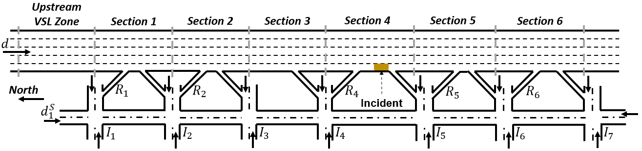
Figure 8: The simulation road network of I-710 freeway and the adjacent arterials. The gold rectangle denotes the location of the incident in some scenarios.

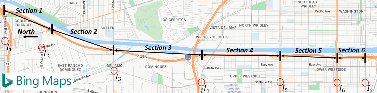
Figure 9: The simulation road network of I-710 freeway and the adjacent arterials on Bing Map. The upstream VSL zone is omitted to save the space.

The turning ratio is determined by the ratio of the traffic flow of each direction, where each traffic flow follows a normal distribution $\mathcal{N}(\mu,\sigma^{2})$. $\mu$ and $\sigma$ are the mean and the standard deviation of the PeMS traffic flow data of the corresponding direction. Although the actual turning ratio is unknown, we use the mean value of the flow distribution to estimate the turning ratio of an intersection approach as follows:

$$y^{t}=\frac{\mu^{t}}{\mu^{l}+\mu^{t}+\mu^{r}}$$ (19)

where $l,t,r$ stand for left-turn, through, right-turn respectively. The turning ratios of on-ramps and off-ramps are estimated in the same manner as those of approaches.

The above-mentioned road network and parameter setting are applied to the online implementation during the learning process of the QL agent. There are 4 scenarios to be executed in one online implemention - moderate demands without incident, moderate demands with incident, high demands without incident, high demands with incident. The cycle of online implementation and continuous learning is repeated 50 times. Then we apply the integrated control for each scenario once more to obtain the final simulation results presented in section IV-B. In addition, we are also interested in 3 other types of control as comparisons. All control strategies to be tested are summarized as follows:

1. No freeway control: inactive VSL, LC and RM control.

2. Decentralized feedback control: a decentralized feedback control strategy proposed in [2].

3. QL without coordination: a QL-based control strategy similar to the proposed one but without coordination. To eliminate the coordination, the arterial traffic states are removed from the state set of the QL algorithm. Moreover, the VSL, LC and RM agent are trained separately.

4. QL with coordination: the proposed control strategy.

IV-B Simulation Results

In this section, we evaluate the performance of 4 types of control strategies as previously mentioned in the road network depicted in Fig. 8 for each interested scenario. The performance criteria are listed as follows [15]:

• Freeway average travel time ($T_{t}$): the average time spent for each vehicle to travel through the freeway segment.

  $$T_{t}=\frac{1}{N_{v}}\sum_{i=1}^{N_{v}}(t_{i,out}-t_{i,in})$$ (20)

  where $N_{v}$ is the number of vehicles passing through the freeway segment, $t_{i,in}$ and $t_{i,out}$ is the time vehicle $i$ enters and exits the freeway segment respectively. $t_{i,in}>10$ min so that the warm-up period is excluded. Vehicles that enter or exit from ramps are also excluded.

• Freeway average number of stops ($\bar{s}$): the average number of stops performed by each vehicle when traveling through the freeway segment.

  $$\bar{s}=\frac{1}{N_{v}}\sum_{i=1}^{N_{v}}s_{i}$$ (21)

  where $s_{i}$ is the number of stops performed by vehicle $i$. The warm-up period is excluded.

• Freeway average emission rates of CO₂ ($E$): the calculation of emission rates is based on the MOVES model provided by the Environment Protection Agency [66].

  $$E=\sum_{i=1}^{N_{v}}E_{i}/\sum_{i=1}^{N_{v}}l_{i}$$ (22)

  where $E_{i}$ is the emission produced by vehicle $i$ and $l_{i}$ is the travelled distance of vehicle $i$. The warm-up period is excluded.

• Average on-ramp queue length ($\bar{w}_{o}$):

  $$\bar{w}_{o}=\sum_{i=1}^{N}\bar{w}_{i}/N_{o}$$ (23)

  where $N$ is the number of freeway sections, $\bar{w}_{i}$ is the average queue length of on-ramp $i$ during the simulation except the warm-up, $N_{o}$ is the number of on-ramps.

• Average queue length of arterial intersections ($\bar{w}_{a}$):

  $$\bar{w}_{a}=\sum_{k=1}^{K}(\bar{w}^{N}_{k}+\bar{w}^{S}_{k}+\bar{w}^{E}_{k}+\bar{w}^{W}_{k})/4K$$ (24)

  where $K$ is the number of arterial intersections, $\bar{w}^{N}_{k}$ is the average queue length of the Northbound approach of intersection $k$ during the simulation except the warm-up.

Considering the stochastic nature of microscopic simulations, we take the average of 10 simulation runs for each pair of control type and scenario and record the final results in Table II, III, IV and V.

TABLE II: Evaluations of a Moderate-Demand Scenario without Incident

Control	$T_{t}$ (min)	$\bar{s}$	$E$ (g/veh/km)	$\bar{w}_{o}$ (m)	$\bar{w}_{a}(m)$
No freeway control	10.2	0.3	200.5	0	11.2
Decentralized feedback control	10.2	0.2	199.8	0	11.9
QL without coordination	10.2	0.2	199.4	0	12.5
QL with coordination	10.2	0.2	200	0	11.6

TABLE III: Evaluations of a Moderate-Demand Scenario with Incident

Control	$T_{t}$ (min)	$\bar{s}$	$E$ (g/veh/km)	$\bar{w}_{o}$ (m)	$\bar{w}_{a}(m)$
No freeway control	12.3	0.7	212.7	0	14.5
Decentralized feedback control	11.4(7%)	0.5(29%)	209(2%)	13.1	11.7
QL without coordination	11.3(8%)	0.5(29%)	208.1(2%)	15.9	11.6
QL with coordination	10.8(12%)	0.3(57%)	203.2(4%)	16.4	11.7

TABLE IV: Evaluations of a High-Demand Scenario without Incident

Control	$T_{t}$ (min)	$\bar{s}$	$E$ (g/veh/km)	$\bar{w}_{o}$ (m)	$\bar{w}_{a}(m)$
No freeway control	12	2.1	241.7	25.3	49.6
Decentralized feedback control	11.7(2%)	1.6(24%)	233.7(3%)	30.2	49.3
QL without coordination	11.6(3%)	1.7(19%)	232.5(4%)	44.1	47.8
QL with coordination	11.3(6%)	1.4(33%)	225.5(7%)	40.8	45.6

TABLE V: Evaluations of a High-Demand Scenario with Incident

Control	$T_{t}$ (min)	$\bar{s}$	$E$ (g/veh/km)	$\bar{w}_{o}$ (m)	$\bar{w}_{a}(m)$
No freeway control	14.1	4.9	262.4	33	56.7
Decentralized feedback control	13(8%)	2.9(41%)	253(4%)	35.9	55.2
QL without coordination	13.3(6%)	3.2(35%)	254.2(3%)	48.7	51
QL with coordination	12.4(12%)	2.4(51%)	245.3(7%)	47	47.5

Table II presents the results of a moderate-demand scenario without incident, where there is no bottleneck on freeway and minimal control effort is needed. Thus, the results of all types of control are close to each other. The average number of stops is supposed to be 0 in reality. However, the stop happens in simulations when two vehicles are very close to each other at ramp merging points. Table III presents the results of a moderate-demand scenario with incident, where the incident introduces a lane-drop bottleneck that increases the travel time ($T_{t}$) and the number of stops ($\bar{s}$) significantly. The percentages in brackets quantify the performance improvement by implementing the corresponding control scheme versus no freeway control. The percentage improvement of QL with coordination is higher than decentralized feedback control and QL without coordination, which verifies the benefit of coordinating different control components. Table IV presents the results of a high-demand scenario without incident, where the increased demand introduces bottlenecks at on-ramp merging areas. The overall performance improvement by freeway traffic control is less obvious compared with Table III because the ramp-merging bottleneck is less detrimental than the lane-drop bottleneck. The coordinated QL still outperforms uncoordinated control schemes with less margins. Table V presents the results of a high-demand scenario with incident, where both the lane-drop bottleneck and ramp-merging bottlenecks exist. The performance margins between coordinated QL and uncoordinated control schemes in Table V are close to those in Table III. The above observations indicate that the proposed coordination mechanism provides higher benefits when the demand grows up or when the incident takes place.

A trade-off between the freeway performance ($T_{t},\bar{s},E$) and on-ramp queue lengths ($\bar{w}_{o}$) can be observed by using any type of freeway traffic control. Taking the coordinated QL in Table V as an example, the average on-ramp queue is 14 m longer while the average freeway travel time is reduced by 12%. The increase in the queue length is trivial considering the minimum on-ramp queue capacity, which is over 300 m. Therefore, the trade-off is acceptable. Besides, the average queue length of arterial intersections ($\bar{w}_{a}$) has no significant change with any type of control in each scenario, which implies that the proposed control strategy relieves the freeway traffic congestion without compromising arterial traffic conditions.

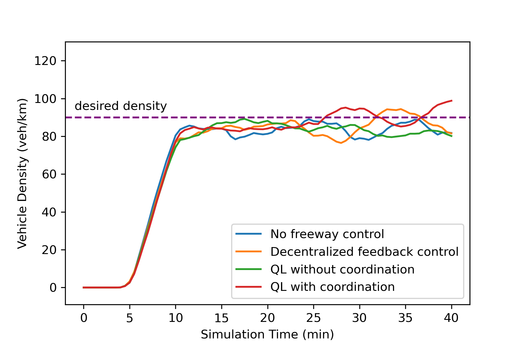
(a)

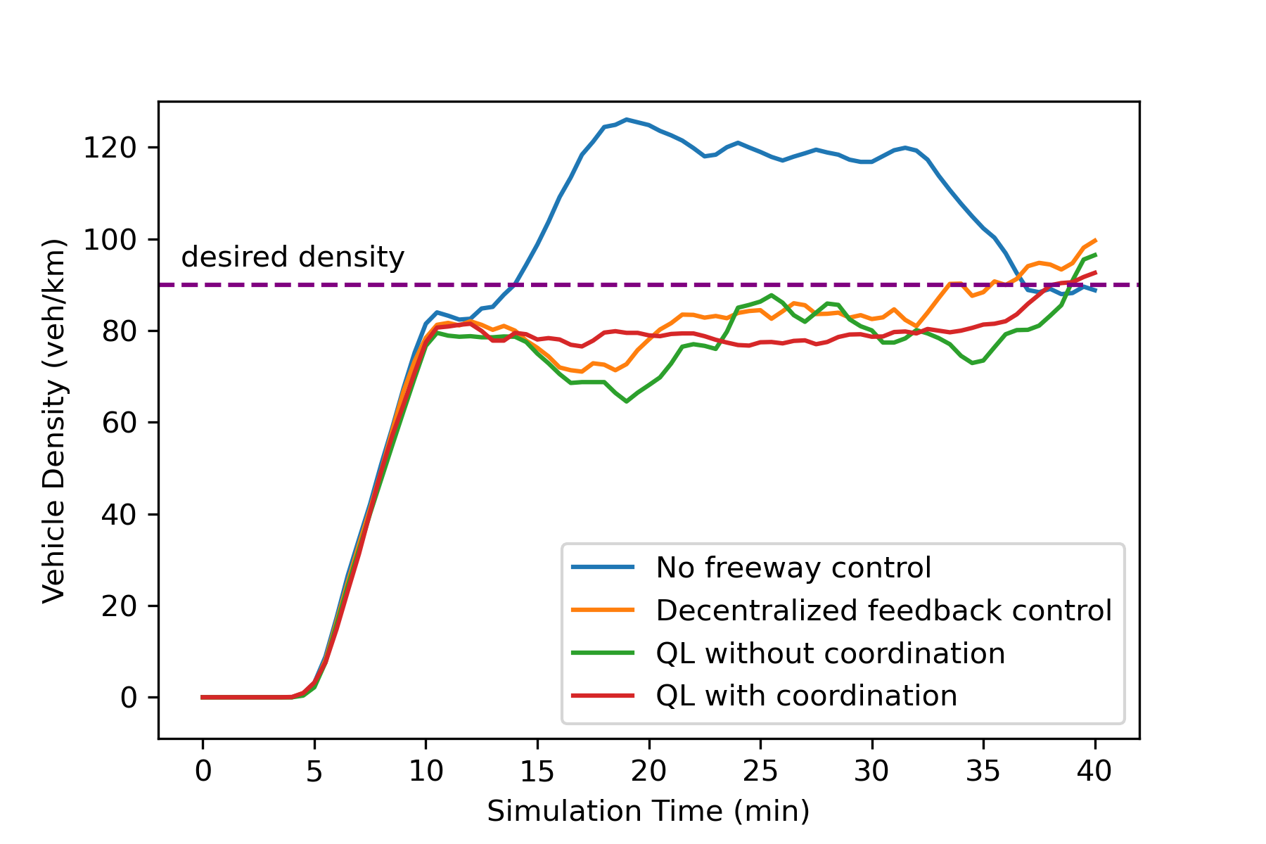
(b)

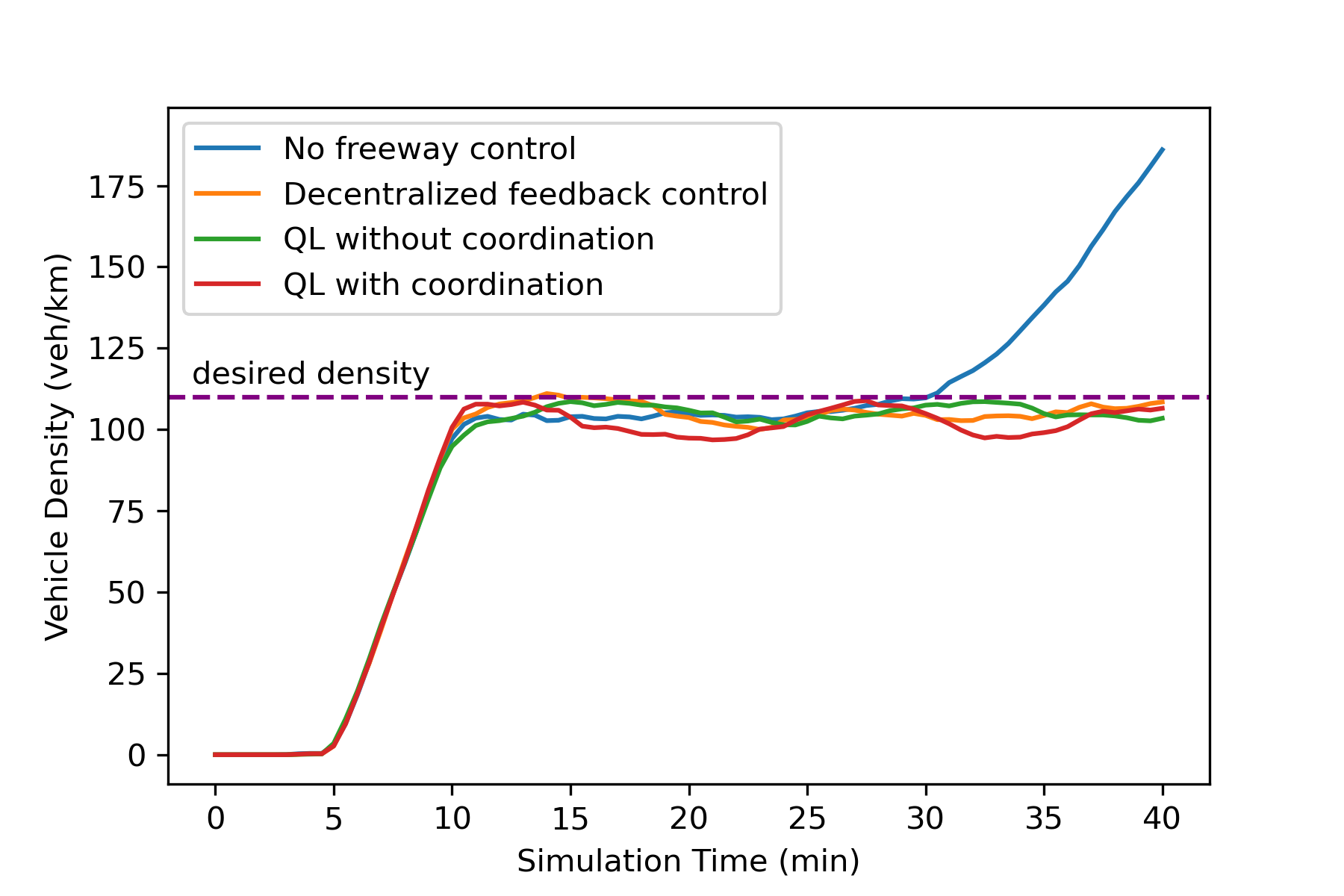
(c)

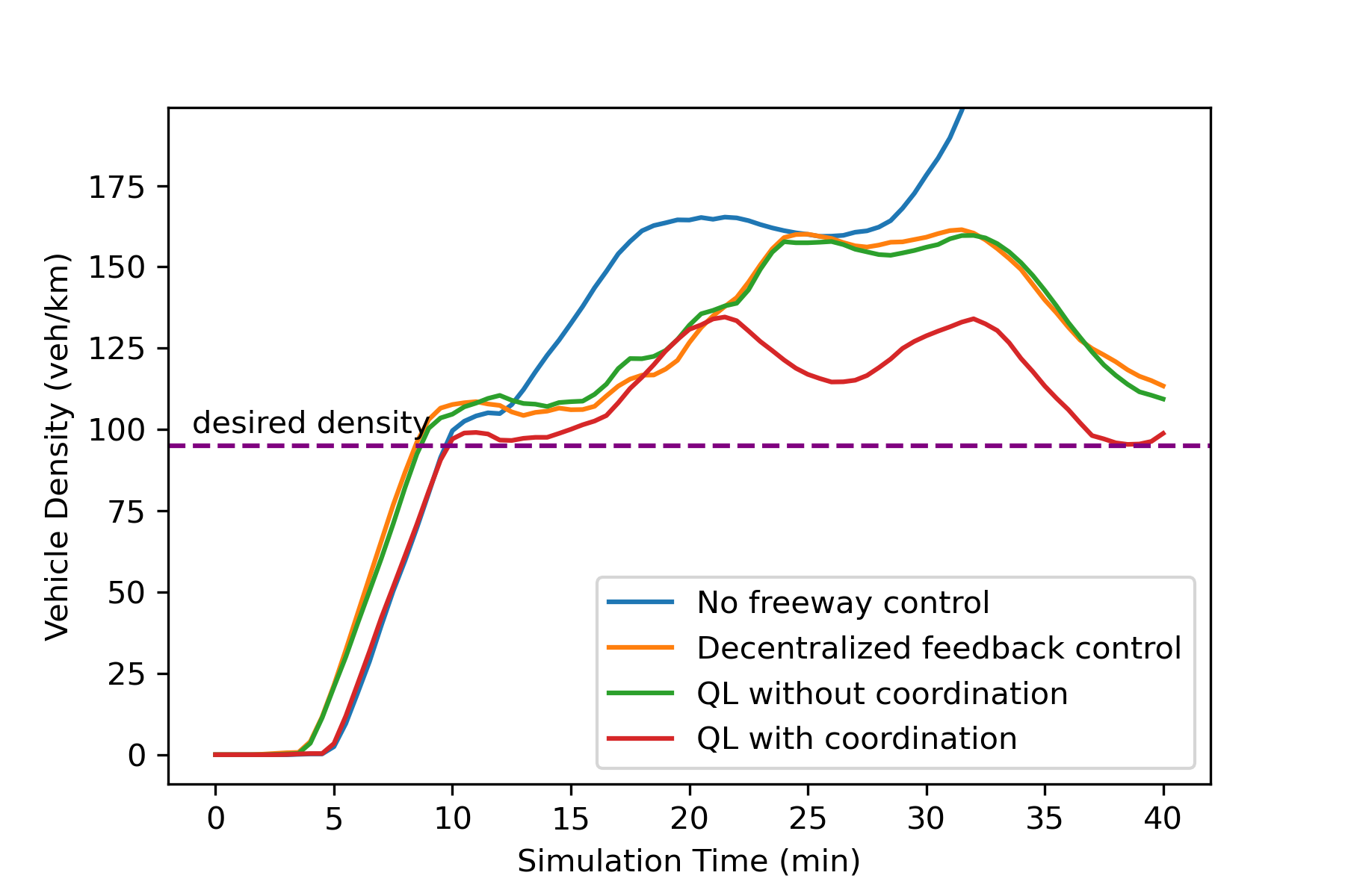
(d)

Figure 10: Measured vehicle density profiles of each scenario in freeway CTM section 4 (where the incident takes place). (a) moderate demand without incident, (b) moderate demand with incident, (c) high demand without incident, (d) high demand with incident.

We draw density profiles for freeway CTM section 4 in Fig. 10 as a representative since the density profiles of each section shares similar behaviors. The purple dash line marks the desired density $\rho^{*}$ in each scenario. We spend a 10-min warm-up loading traffic for the entire network. Then the control algorithm kicks in and maintains the density of each CTM section at the steady state. Fig. 10 shows that the interested control schemes deliver similar performance in terms of stabilizing the density when there is no incident. The coordinated QL performs significantly better than the uncoordinated QL and decentralized feedback control when the incident occurs in high-demand scenarios. The above results also demonstrate the necessity of coordinating different control components when the road network is congested.

V Conclusion

In this paper, we proposed an integrated freeway and arterial traffic control strategy that coordinates the variable speed limit (VSL) control, the lane change (LC) recommendations, the ramp metering (RM) and the traffic signal control (TSC) using Q-learning (QL). The QL agent is trained offline in a single-section road network first, and then implemented online in the I-710 simulation road network with real-world traffic demands from PeMS. The online data are collected to assist the continuous learning of the QL agent. The cycle of the online implementation and the continuous learning are iterated multiple times to further improve the control performance. The arterial signal plans are determined by simulation-based cycle length models and estimated demands of all intersection approaches in a traffic-responsive manner. To facilitate the coordination, the signal plan and estimated demands of adjacent arterial intersections are involved in the state set of the QL algorithm. The numerical simulations indicate that the proposed approach achieves higher performance in the freeway part compared with uncoordinated QL or decentralized feedback control in high-demand or incident scenarios. Meanwhile, the on-ramp queue increases slightly as an acceptable trade-off and the queues at arterial intersections stay at the same level. The freeway density profiles also verify the benefits of coordinating different control components when the incident exists and the road network is congested.

In the future, we plan to incorporate signal offset and speed advisory in arterial traffic control to maximize the progression bandwidth and reduce arterial travel delays. The problem can be potentially solved using a similar QL framework.

Tianchen Yuan received the B.Sc. degree with distinction and the M.S. degree both in Electrical Engineering from University of Minnesota, Minneapolis, USA, in 2015 and 2017, respectively. He is currently working toward a Ph.D. degree with the Center of Advanced Transportation Technology, University of Southern California, Los Angeles, CA, USA. His research topics involve intelligent transportation systems, traffic flow control and optimizations.

Petros A. Ioannou (Life Fellow, IEEE) received the B.Sc. degree (Hons.) from University College, London, England, in 1978, and the M.S. and Ph.D. degrees from the University of Illinois at Urbana, IL, USA, in 1980 and 1982, respectively. In 1982, he joined the Department of Electrical Engineering-Systems, University of Southern California, Los Angeles, CA, USA. He is currently a Professor and the holder of the AV ’Bal’ Balakrishnan Chair with the Department of Electrical Engineering-Systems, the Director of the Center of Advanced Transportation Technologies, and an Associate Director for Research of METRANS. He also holds a courtesy appointment with the Departments of Aerospace, Mechanical Engineering and Industrial System Engineering. His research interests are in the areas of adaptive control, neural networks, nonlinear systems, vehicle dynamics and control, intelligent transportation systems, and marine transportation. He is a fellow of IFAC, AAAS, and Life Fellow of IEEE and author/coauthor of nine books and over 400 papers in the areas of control, vehicle dynamics, and intelligent transportation systems. He is a member of the National Academy of Engineering, Fellow of the National Academy of Inventors and foreign member of the Academy Europaea.

References

- [1] R. C. Carlson, I. Papamichail, M. Papageorgiou, and A. Messmer, “Optimal motorway traffic flow control involving variable speed limits and ramp metering,” Transportation science, vol. 44, no. 2, pp. 238–253, 2010.
- [2] Y. Zhang and P. A. Ioannou, “Integrated control of highway traffic flow,” Journal of Control and Decision, vol. 5, no. 1, pp. 19–41, 2018.
- [3] J. R. D. Frejo and B. De Schutter, “Logic-based traffic flow control for ramp metering and variable speed limits—part 1: Controller,” IEEE Transactions on Intelligent Transportation Systems, vol. 22, no. 5, pp. 2647–2657, 2020.
- [4] G. De Nunzio, G. Gomes, C. Canudas-de Wit, R. Horowitz, and P. Moulin, “Speed advisory and signal offsets control for arterial bandwidth maximization and energy consumption reduction,” IEEE Transactions on Control Systems Technology, vol. 25, no. 3, pp. 875–887, 2016.
- [5] P. Wang, Y. Jiang, L. Xiao, Y. Zhao, and Y. Li, “A joint control model for connected vehicle platoon and arterial signal coordination,” Journal of Intelligent Transportation Systems, vol. 24, no. 1, pp. 81–92, 2020.
- [6] H. Wang and X. Peng, “Coordinated control model for oversaturated arterial intersections,” IEEE Transactions on Intelligent Transportation Systems, 2022.
- [7] T. Urbanik, D. Humphreys, B. Smith, S. Levine et al., “Coordinated freeway and arterial operations handbook,” United States. Federal Highway Administration, Tech. Rep., 2006.
- [8] M. Van den Berg, A. Hegyi, B. De Schutter, and H. Hellendoorn, “Integrated traffic control for mixed urban and freeway networks: A model predictive control approach,” European journal of transport and infrastructure research, vol. 7, no. 3, 2007.
- [9] J. Haddad, M. Ramezani, and N. Geroliminis, “Cooperative traffic control of a mixed network with two urban regions and a freeway,” Transportation Research Part B: Methodological, vol. 54, pp. 17–36, 2013.
- [10] D. Su, X.-Y. Lu, R. Horowitz, and Z. Wang, “Coordinated ramp metering and intersection signal control,” International Journal of Transportation Science and Technology, vol. 3, no. 2, pp. 179–192, 2014.
- [11] T. Yuan, F. Alasiri, and P. A. Ioannou, “Selection of the speed command distance for improved performance of a rule-based vsl and lane change control,” IEEE Transactions on Intelligent Transportation Systems, 2022.
- [12] E. Kwon, D. Brannan, K. Shouman, C. Isackson, and B. Arseneau, “Development and field evaluation of variable advisory speed limit system for work zones,” Transportation research record, vol. 2015, no. 1, pp. 12–18, 2007.
- [13] J. M. Torné Santos, D. M. Rosas Díaz, and F. Soriguera Martí, “Evaluation of speed limit management on c-32 highway access to barcelona,” in Proceedings of the TRB 90th Annual Meeting, 2011, pp. 1–23.
- [14] M. Hadiuzzaman and T. Z. Qiu, “Cell transmission model based variable speed limit control for freeways,” Canadian Journal of Civil Engineering, vol. 40, no. 1, pp. 46–56, 2013.
- [15] Y. Zhang and P. A. Ioannou, “Combined variable speed limit and lane change control for highway traffic,” IEEE Transactions on Intelligent Transportation Systems, vol. 18, no. 7, pp. 1812–1823, 2017.
- [16] M. Papageorgiou, H. Hadj-Salem, J.-M. Blosseville et al., “Alinea: A local feedback control law for on-ramp metering,” Transportation Research Record, vol. 1320, no. 1, pp. 58–67, 1991.
- [17] E. Smaragdis and M. Papageorgiou, “Series of new local ramp metering strategies: Emmanouil smaragdis and markos papageorgiou,” Transportation Research Record, vol. 1856, no. 1, pp. 74–86, 2003.
- [18] Y. Wang and M. Papageorgiou, “Local ramp metering in the case of distant downstream bottlenecks,” in 2006 IEEE Intelligent Transportation Systems Conference. IEEE, 2006, pp. 426–431.
- [19] S. Smulders, “Control of freeway traffic flow by variable speed signs,” Transportation Research Part B: Methodological, vol. 24, no. 2, pp. 111–132, 1990.
- [20] H. Zackor, “Speed limitation on freeways: Traffic-responsive strategies,” in Concise Encyclopedia of Traffic & Transportation Systems. Elsevier, 1991, pp. 507–511.
- [21] A. Hegyi, B. De Schutter, and J. Heelendoorn, “Mpc-based optimal coordination of variable speed limits to suppress shock waves in freeway traffic,” in Proceedings of the 2003 American Control Conference, 2003., vol. 5. IEEE, 2003, pp. 4083–4088.
- [22] J. R. D. Frejo, A. Núñez, B. De Schutter, and E. F. Camacho, “Hybrid model predictive control for freeway traffic using discrete speed limit signals,” Transportation Research Part C: Emerging Technologies, vol. 46, pp. 309–325, 2014.
- [23] B. Khondaker and L. Kattan, “Variable speed limit: A microscopic analysis in a connected vehicle environment,” Transportation Research Part C: Emerging Technologies, vol. 58, pp. 146–159, 2015.
- [24] A. Muralidharan and R. Horowitz, “Computationally efficient model predictive control of freeway networks,” Transportation Research Part C: Emerging Technologies, vol. 58, pp. 532–553, 2015.
- [25] R. C. Carlson, I. Papamichail, and M. Papageorgiou, “Comparison of local feedback controllers for the mainstream traffic flow on freeways using variable speed limits,” Journal of Intelligent Transportation Systems, vol. 17, no. 4, pp. 268–281, 2013.
- [26] G.-R. Iordanidou, C. Roncoli, I. Papamichail, and M. Papageorgiou, “Feedback-based mainstream traffic flow control for multiple bottlenecks on motorways,” IEEE Transactions on Intelligent Transportation Systems, vol. 16, no. 2, pp. 610–621, 2014.
- [27] H.-Y. Jin and W.-L. Jin, “Control of a lane-drop bottleneck through variable speed limits,” Transportation Research Part C: Emerging Technologies, vol. 58, pp. 568–584, 2015.
- [28] Y. Zhang and P. A. Ioannou, “Stability analysis and variable speed limit control of a traffic flow model,” Transportation Research Part B: Methodological, vol. 118, pp. 31–65, 2018.
- [29] T. Yuan, F. Alasiri, Y. Zhang, and P. A. Ioannou, “Evaluation of integrated variable speed limit and lane change control for highway traffic flow,” IFAC-PapersOnLine, vol. 54, no. 2, pp. 107–113, 2021.
- [30] F. Alasiri, Y. Zhang, and P. A. Ioannou, “Robust variable speed limit control with respect to uncertainties,” European Journal of Control, 2020.
- [31] E. Walraven, M. T. Spaan, and B. Bakker, “Traffic flow optimization: A reinforcement learning approach,” Engineering Applications of Artificial Intelligence, vol. 52, pp. 203–212, 2016.
- [32] Z. Li, P. Liu, C. Xu, H. Duan, and W. Wang, “Reinforcement learning-based variable speed limit control strategy to reduce traffic congestion at freeway recurrent bottlenecks,” IEEE transactions on intelligent transportation systems, vol. 18, no. 11, pp. 3204–3217, 2017.
- [33] C. Roncoli, N. Bekiaris-Liberis, and M. Papageorgiou, “Optimal lane-changing control at motorway bottlenecks,” in 2016 IEEE 19th International Conference on Intelligent Transportation Systems (ITSC). IEEE, 2016, pp. 1785–1791.
- [34] F. Alasiri, Y. Zhang, and P. A. Ioannou, “Per-lane variable speed limit and lane change control for congestion management at bottlenecks,” IEEE Transactions on Intelligent Transportation Systems, 2023.
- [35] Y. Guo, H. Xu, Y. Zhang, and D. Yao, “Integrated variable speed limits and lane-changing control for freeway lane-drop bottlenecks,” IEEE Access, vol. 8, pp. 54 710–54 721, 2020.
- [36] F. Tajdari, C. Roncoli, and M. Papageorgiou, “Feedback-based ramp metering and lane-changing control with connected and automated vehicles,” IEEE Transactions on Intelligent Transportation Systems, vol. 23, no. 2, pp. 939–951, 2020.
- [37] Y. Kim, D. Ka, and C. Lee, “Lane-changing control with balancing lane flow at freeway merge bottlenecks in a connected vehicle environment: Application of a pid controller,” IET Intelligent Transport Systems, 2023.
- [38] Y. J. Stephanedes, “Implementation of on-line zone control strategies for optimal ramp metering in the minneapolis ring road,” 1994.
- [39] H. M. Zhang and S. G. Ritchie, “Freeway ramp metering using artificial neural networks,” Transportation Research Part C: Emerging Technologies, vol. 5, no. 5, pp. 273–286, 1997.
- [40] G. Paesani, J. Kerr, P. Perovich, and F. Khosravi, “System wide adaptive ramp metering (swarm),” in Merging the Transportation and Communications Revolutions. Abstracts for ITS America Seventh Annual Meeting and ExpositionITS America, 1997.
- [41] I. Papamichail, M. Papageorgiou, V. Vong, and J. Gaffney, “Heuristic ramp-metering coordination strategy implemented at monash freeway, australia,” Transportation Research Record, vol. 2178, no. 1, pp. 10–20, 2010.
- [42] Y. Han, M. Ramezani, A. Hegyi, Y. Yuan, and S. Hoogendoorn, “Hierarchical ramp metering in freeways: an aggregated modeling and control approach,” Transportation research part C: emerging technologies, vol. 110, pp. 1–19, 2020.
- [43] F. V. Webster, “Traffic signal settings,” Tech. Rep., 1958.
- [44] F. Webster, “Traffic signals,” Road research technical paper, vol. 56, 1966.
- [45] J. D. Little, M. D. Kelson, and N. H. Gartner, “Maxband: A versatile program for setting signals on arteries and triangular networks,” 1981.
- [46] D. I. Robertson, “’tansyt’method for area traffic control,” Traffic Engineering & Control, vol. 8, no. 8, 1969.
- [47] N. H. Gartner, S. F. Assman, F. Lasaga, and D. L. Hou, “A multi-band approach to arterial traffic signal optimization,” Transportation Research Part B: Methodological, vol. 25, no. 1, pp. 55–74, 1991.
- [48] T. Arsava, Y. Xie, and N. H. Gartner, “Arterial progression optimization using od-band: case study and extensions,” Transportation Research Record, vol. 2558, no. 1, pp. 1–10, 2016.
- [49] P. Hunt, D. Robertson, R. Bretherton, and M. C. Royle, “The scoot on-line traffic signal optimisation technique,” Traffic Engineering & Control, vol. 23, no. 4, 1982.
- [50] P. Mirchandani and F.-Y. Wang, “Rhodes to intelligent transportation systems,” IEEE Intelligent Systems, vol. 20, no. 1, pp. 10–15, 2005.
- [51] I. Schelling, A. Hegyi, and S. P. Hoogendoorn, “Specialist-rm—integrated variable speed limit control and ramp metering based on shock wave theory,” in 2011 14th International IEEE conference on intelligent transportation systems (ITSC). IEEE, 2011, pp. 2154–2159.
- [52] G.-R. Iordanidou, I. Papamichail, C. Roncoli, and M. Papageorgiou, “Feedback-based integrated motorway traffic flow control with delay balancing,” IEEE Transactions on Intelligent Transportation Systems, vol. 18, no. 9, pp. 2319–2329, 2017.
- [53] T. Schmidt-Dumont and J. H. van Vuuren, “Decentralised reinforcement learning for ramp metering and variable speed limits on highways,” IEEE Transactions on Intelligent Transportation Systems, vol. 14, no. 8, p. 1, 2015.
- [54] A. Srivastava and W. Jin, “A lane changing cell transmission model for modeling capacity drop at lane drop bottlenecks,” Tech. Rep., 2016.
- [55] C. J. Watkins and P. Dayan, “Q-learning,” Machine learning, vol. 8, pp. 279–292, 1992.
- [56] C. F. Daganzo, “The cell transmission model: A dynamic representation of highway traffic consistent with the hydrodynamic theory,” Transportation Research Part B: Methodological, vol. 28, no. 4, pp. 269–287, 1994.
- [57] ——, “The cell transmission model, part II: network traffic,” Transportation Research Part B: Methodological, vol. 29, no. 2, pp. 79–93, 1995.
- [58] M. Kontorinaki, A. Spiliopoulou, C. Roncoli, and M. Papageorgiou, “First-order traffic flow models incorporating capacity drop: Overview and real-data validation,” Transportation Research Part B: Methodological, vol. 106, pp. 52–75, 2017.
- [59] M. J. Lighthill and G. B. Whitham, “On kinematic waves II. a theory of traffic flow on long crowded roads,” Proceedings of the Royal Society of London. Series A. Mathematical and Physical Sciences, vol. 229, no. 1178, pp. 317–345, 1955.
- [60] P. I. Richards, “Shock waves on the highway,” Operations research, vol. 4, no. 1, pp. 42–51, 1956.
- [61] F. L. Hall and K. Agyemang-Duah, “Freeway capacity drop and the definition of capacity,” Transportation research record, no. 1320, 1991.
- [62] X. Li, G. Li, S.-S. Pang, X. Yang, and J. Tian, “Signal timing of intersections using integrated optimization of traffic quality, emissions and fuel consumption: a note,” Transportation Research Part D: Transport and Environment, vol. 9, no. 5, pp. 401–407, 2004.
- [63] A. Hajbabaie and R. F. Benekohal, “Traffic signal timing optimization: Choosing the objective function,” Transportation research record, vol. 2355, no. 1, pp. 10–19, 2013.
- [64] A. J. Calle-Laguna, J. Du, and H. A. Rakha, “Computing optimum traffic signal cycle length considering vehicle delay and fuel consumption,” Transportation Research Interdisciplinary Perspectives, vol. 3, p. 100021, 2019.
- [65] J. A. Bonneson and M. D. Fontaine, “Evaluating intersection improvements: an engineering study guide,” 2001.
- [66] U. Epa, “Motor vehicle emission simulator (moves) user guide,” US Environmental Protection Agency, 2010.