Interferometric Neural Networks

Abstract

On the one hand, artificial neural networks have many successful applications in the field of machine learning and optimization. On the other hand, interferometers are integral parts of any field that deals with waves such as optics, astronomy, and quantum physics. Here, we introduce neural networks composed of interferometers and then build generative adversarial networks from them. Our networks do not have any classical layer and can be realized on quantum computers or photonic chips. We demonstrate their applicability for combinatorial optimization, image classification, and image generation. For combinatorial optimization, our network consistently converges to the global optimum or remains within a narrow range of it. In multi-class image classification tasks, our networks achieve accuracies of ${93\%}$ and ${83\%}$. Lastly, we show their capability to generate images of digits from 0 to 9 as well as human faces.

I Introduction

Artificial neural networks (NNs) LeCun15 ; Goodfellow16 ; Aggarwal23 have demonstrated remarkable success in a wide range of applications in various domains such as autonomous vehicles, healthcare, finance, robotics, gaming, over-the-top media services, and chatbots. Some of the applications include image classification Lecun89 ; Lecun98 ; Krizhevsky12 , natural language processing, speech recognition, robotic control systems, recommendation systems, and image generation Goodfellow14 ; Radford15 ; Arjovsky17 ; Gulrajani17 . Convolutional NNs (CNNs) were introduced in Lecun89 ; Lecun98 and further improved in seminal works like Krizhevsky12 for image classification. Similarly, generative adversarial networks (GANs) made their debut in Goodfellow14 and underwent notable advancements in subsequent works, including Radford15 ; Arjovsky17 ; Gulrajani17 for image generation. In this paper, we introduce interferometric NNs (INNs) consisting of interferometers in Sec. II and then interferometric GANs (IGANs) composed of INNs in Sec. III.

Interferometers play a pivotal role in metrology, astronomy, optics, and quantum physics. Feynman, in his renowned lectures, introduced quantum (wave-particle) behavior through double-slit (two-path) interference experiments Feynman64 . The wave-particle duality, a subject of the famous Bohr-Einstein debates, has been further investigated by numerous scientists using two- and multi-path interferometers (for instance, see Wootters79 ; Greenberger88 ; Englert96 ; Durr98a ; Durr98b ; Englert08 ; Coles16 ; Qureshi17 ). Our INNs are made of sequences of such multi-path interferometers, where each interferometer is a combination of beamsplitters (or fiber couplers) and a phase shifter Englert96 ; Englert08 ; Coles16 ; Weihs16 . A beamsplitter is represented by a discrete Fourier transformation, and the phase shifters hold all the learnable parameters of an INN. In principle, an INN can work with classical or quantum waves. However, a sequence of interferometers can be viewed as a parameterized quantum circuit (PQC), where a Fourier transformation can be implemented exponentially faster than its classical counterpart thanks to Peter Shor Shor96 .

The PQCs Benedetti19 are integral components of the variational quantum algorithms (VQAs), including the variational quantum eigensolver (VQE) Peruzzo14 ; McClean16 and its variants Malley16 ; Motta18 ; Lee19 ; Matsuzawa20 for determining molecular energies and the quantum approximate optimization algorithm (QAOA) Farhi14 for solving combinatorial optimization problems by recasting them as energy minimization in Ising spin glass systems Lucas14 . Recognizing that fully fault-tolerant quantum computers may still be decades away, VQAs are harnessing the capabilities of today’s noisy intermediate-scale quantum (NISQ) computers Preskill18 by providing a framework to build a wide range of applications. Some of these applications include finding ground Peruzzo14 ; McClean16 and excited Higgott19 ; Nakanishi19 energy states, combinatorial optimization Farhi14 ; Lucas14 , simulating quantum dynamics Li17 ; Yuan19 ; Cirstoiu20 ; Gibbs21 ; Kivlichan18 , solving a system of linear Bravo-Prieto19 ; Huang19 ; Xu21 and non-linear Lubasch20 ; Kyriienko21 equations, data classification Farhi18 ; Havlicek19 ; Franken20 ; Mitarai18 ; Huggins19 ; Grant18 ; Schuld19 ; Schuld20 , and generative tasks Romero17 ; Lloyd18 ; Demers18 ; Zoufal19 ; Romero19 ; Niu21 ; Huang21 ; Tsang22 ; Zhou23 ; Stein21 ; Chu22 ; Liu18 ; Benedetti19b ; Coyle20 ; Rudolph22 ; Tian22 . For an in-depth review of VQAs and NISQ algorithms, we refer readers to Cerezo21 ; Bharti22 . An INN also belongs to the VQA family, as it can provide an ansatz for a VQA.

We employ INNs for combinatorial optimization and image classification in Sec. II and IGANs for image generation in Sec. III. The notion of quantum GANs was initially introduced in Lloyd18 and numerically implemented in Demers18 using PQCs. Subsequently, various quantum GANs have been proposed to generate samples from random distributions Zoufal19 ; Romero19 ; Niu21 , as well as to generate images Huang21 ; Tsang22 ; Zhou23 ; Stein21 ; Chu22 . Leveraging the Born rule, which provides a probability distribution from a (parameterized) quantum state, PQCs as Born machines Liu18 ; Benedetti19b ; Coyle20 ; Rudolph22 are utilized for these generative tasks.

We provide a summary of our contributions at the beginning of the next two sections and an overarching conclusion and outlook in Sec. IV. One can find a dedicated Jupyter Notebook for each of the problems discussed in this paper within our GitHub repository Arun_GitHub . These problems are tackled using INNs, which are classically simulated in the PyTorch machine-learning framework Paszke19 . PyTorch automatically manages the gradient of a loss or an energy function. For the training of each INN, we employ the Adam optimizer Kingma14 .

II INN

In this section, our primary contributions are in (II)–(II), (II), Figs. 1–5, Table 1, and Arun_GitHub . Here we introduce INNs through (II)–(II), (II), Figs. 1, 4, and 5. Initially applied to specific combinatorial optimization problems, we illustrate their performance in Fig. 2. Subsequently, we use them for image classification tasks, and their performance is detailed in Fig. 3 and Table 1.

The INN in Fig. 1 is made of a sequence of interferometers, where each interferometer has $d$ distinct paths represented by the computation (orthonormal) basis

$$\mathcal{B}=\big{\{}|0\rangle,\cdots,|d-1\rangle\big{\}}$$ (1)

of the associated Hilbert space. Basically, this whole setup is a $d$-level quantum computer. In the case of $d=2^{n}$, one can construct an equivalent PQC of $n$ qubits ($2$-level quantum systems) as shown in Fig. 1.

In a machine-learning task, one has to feed the data to a NN, and the data is a collection of feature vectors $\textbf{x}=(x_{0},\cdots,x_{d-1})\in\mathbb{R}^{d}$. Whereas, in the case of INN, we have to encode every x into an input state vector $|\textbf{x}\rangle$ through a unitary transformation. Such a process is called feature encoding Schuld20 . Throughout the paper, we consider the amplitude encoding

$$|\textbf{x}\rangle=\frac{1}{\|\textbf{x}\|}\sum_{j=0}^{d-1}x_{j}\,|j\rangle\,,$$ (2)

where $\|\textbf{x}\|$ is the Euclidean norm of x.

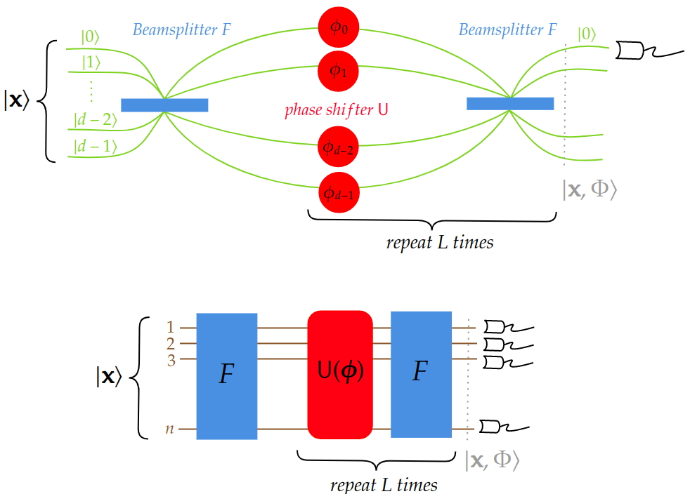
Figure 1: The top and bottom pictures show an INN and its equivalent PQC in the case of $d=2^{n}$, respectively. The INN is a sequence of $L$ interferometers, where the output from one is fed to the next. Each interferometer has $d$ distinct paths colored in green, beamsplitters (or fiber couplers) exhibited by blue-colored slabs, and a phase shifter shown by red disks in the top picture. In the bottom picture, brown wires depict $n$ qubits, and the beamsplitter and phase shifter are displayed by blue and red-rounded rectangles, respectively. An input to the INN or to the PQC is a ket ${|\textbf{x}\rangle}$ from (2), the beamsplitter $F$ and phase shifters $U(\bm{\phi}^{l})$ are given in (II), and the output ${|\textbf{x},\Phi\rangle}$ is read by the detectors shown in black. The whole setup is summarized in (II).

As shown in Fig. 1 following Englert96 ; Englert08 ; Coles16 ; Weihs16 , an interferometer has two essential elements: beamsplitters (or fiber couplers) and a phase shifter, which, in our case, are mathematically described by the unitary operators

$$F =\frac{1}{\sqrt{d}}\sum_{k=0}^{d-1}\sum_{j=0}^{d-1}\omega^{\,kj}\,|k\rangle\langle j|\quad\mbox{and}$$

$$U(\bm{\phi}) =\sum_{j=0}^{d-1}\text{e}^{\texttt{i}\phi_{j}}|j\rangle\langle j|\,,$$ (3)

respectively. In (II), ${\omega=\text{e}^{\texttt{i}\frac{2\pi}{d}}}$ is a $d$th root of unity, $\texttt{i}=\sqrt{-1}$, and $\bm{\phi}=(\phi_{0},\cdots,\phi_{d-1})\in\mathbb{R}^{d}$ carry phases. Here the discrete Fourier transformation $F$ acts as a generalization of a symmetric $50/50$ beamsplitter for a $2$-path interferometer. It turns a single path $|j\rangle$ into an equal superposition of all the paths of $\mathcal{B}$. The phase shifter $U(\bm{\phi})$ shifts the phase by $\phi_{j}$ in the $j$th path. By the way, using the operators from (II), one can realize a phase encoding $|\textbf{x}\rangle_{\text{ph}}=U(\textbf{x})F|0\rangle$ of the data, which might be useful in some applications. We want to emphasize that two layers of the Hadamard and diagonal unitary operations like $U$ are used in Havlicek19 to present a feature map that is hard to simulate classically. Additionally, parameterized diagonal unitary operations such as $U(\bm{\phi})$ have been employed to make a quantum simulation faster in Cirstoiu20 ; Gibbs21 (see also Kivlichan18 ).

For every problem, we have executed $F$ in Arun_GitHub , utilizing the fast Fourier transform available in PyTorch. However, its implementation can reach exponential speedup on a quantum computer due to Shor’s algorithm for quantum Fourier transforms Shor96 . The phase shifter can be decomposed as a product of controlled-phase gates Kivlichan18 :

$$U(\bm{\phi}) =\prod_{j=0}^{d-1}\textsc{cp}(\phi_{j})\,,\quad\mbox{where}$$

$$\textsc{cp}(\phi_{j}) =\text{e}^{\texttt{i}\phi_{j}}|j\rangle\langle j|+\big{(}I-|j\rangle\langle j|\,\big{)}=\text{e}^{\texttt{i}\phi_{j}|j\rangle\langle j|}$$ (4)

and $I$ is the identity operator. In the case of $d=2^{n}$, with the binary representation of integers $j=\sum_{\mu=1}^{n}2^{n-\mu}j_{\mu}$ and association $|j\rangle\equiv\otimes_{\mu=1}^{n}|j_{\mu}\rangle$, one can show that cp is indeed a controlled-phase gate with $n-1$ control qubits. Although there are exponentially many cp gates relative to $n$ in the decomposition, they can all, in principle, be simultaneously realized due to their commutativity. By the way, for $\phi_{j}=\pi$, $\textsc{cp}(\phi_{j})$ becomes a quantum oracle of Grover’s algorithm Grover97 .

Now, we have all the elements to describe the INN of Fig. 1. The INN is made of $L$ layers of interferometers, where the output from one is fed to the next. An input to the first interferometer is $|\textbf{x}\rangle$ from (2), the output from the last one is

$$|\textbf{x},\Phi\rangle =\left(\prod_{l=1}^{L}FU(\bm{\phi}^{l})\right)F\,|\textbf{x}\rangle\,,\quad\mbox{and}$$

$$p =|\langle 0|\textbf{x},\Phi\rangle|^{2}$$ (5)

is the probability of getting $0$th outcome (that is, detecting quantum particles in the $0$th path). Equivalently, in the case of $n$ qubits, we have to perform measurements on all the qubits to get $p$ as $|0\rangle\equiv|0\cdots 0\rangle$ in the binary representation. Equations in (II) completely specify the INN in Fig. 1, and all its learnable parameters are denoted by $\Phi=(\bm{\phi}^{1},\cdots,\bm{\phi}^{L})\in\mathbb{R}^{L\times d}$, which carries $L$ phase-vectors, one for each interferometer.

One can view the INN as a differentiable function $p:\mathbb{R}^{L\times d}\rightarrow[0,1]$ on the parameter space. In optimization or machine-learning tasks, PyTorch automatically manages the gradient computation of an energy or a loss function [given in (8), (11), and (III)] of $p$ with respect to parameter updates. Without such a framework, we would need to compute derivatives such as

$$\frac{\partial p}{\partial\phi^{l}_{j}}=\langle\textbf{x}|\cdots\partial_{j}U^{\dagger}(\bm{\phi}^{l})\cdots|0\rangle\langle 0|\cdots U(\bm{\phi}^{l})\cdots|\textbf{x}\rangle\ +\quad$$

$$\qquad\quad\,\langle\textbf{x}|\cdots U^{\dagger}(\bm{\phi}^{l})\cdots|0\rangle\langle 0|\cdots\partial_{j}U(\bm{\phi}^{l})\cdots|\textbf{x}\rangle\,,\ \mbox{where}$$

$$\partial_{j}U(\bm{\phi}^{l})=\frac{\partial U}{\partial\phi^{l}_{j}}=\texttt{i}\,\text{e}^{\texttt{i}\phi^{l}_{j}}|j\rangle\langle j|=\frac{\partial\textsc{cp}(\phi^{l}_{j})}{\partial\phi^{l}_{j}}\,.$$ (6)

The second equation in (II) expresses the derivative of the $l$th phase shifter with respect to the phase $\phi^{l}_{j}$, and it also turns out to be the derivative of the cp operator. Similarly, one can get the derivative $\partial_{j}U^{\dagger}(\bm{\phi}^{l})$ of the adjoint (denoted by $\dagger$) of $U$.

Now, we demonstrate applications of the INN first for quadratic unconstrained binary optimization (QUBO) and then for classification. A $n$-variable QUBO problem is equivalent to finding a minimum energy eigenstate of an associated $n$-qubit Hamiltonian (for many such problems, see Lucas14 )

$$H=\sum_{\mu,\nu=1}^{n}\mathsf{Q}_{\mu\nu}P_{\mu}P_{\nu}\,,$$ (7)

where $\mathsf{Q}$ is a $n\times n$ real matrix that defines the problem, and the projector $P_{\mu}$ acts on the $\mu$th qubit as $P_{\mu}|j_{\mu}\rangle=j_{\mu}|j_{\mu}\rangle\,,j_{\mu}\in\{0,1\}$. By the binary representation $j=\sum_{\mu}2^{n-\mu}j_{\mu}$ and $|j\rangle\equiv\otimes_{\mu}|j_{\mu}\rangle$, $H$ is diagonal in the computational basis $\mathcal{B}$ of (1). The global minimum will be $E_{j}=\langle j|H|j\rangle$ for some $j\in\{0,\cdots,d-1\}$. Since $\{E_{j}\}$ does not have any structure like convex functions, finding the minimum out of exponentially ($d=2^{n}$) many possibilities is an NP-hard problem.

Several successful VQAs, including the VQE Peruzzo14 ; McClean16 and QAOA Farhi14 , have been proposed to find good approximate solutions. Their basic structure involves preparing a parametric state (referred as ansatz), computing and minimizing the energy expectation value, and obtaining an approximate solution from the optimized ansatz. A QAOA ansatz is constructed by sequentially applying the problem and a mixer unitary operators, whereas the VQE ansatz is generated by applying unitary coupled cluster operators to an initialized state (for more details, see McClean16 ; Cerezo21 ; Bharti22 ). Our approach is similar as narrated next, with the key distinction being that our ansatz is derived from the INN of Fig. 1.

We start with the input ket $|\textbf{x}\rangle=|0\rangle$ and reach the output ket $|0,\Phi\rangle\equiv|\Phi\rangle$ as per (II). Then we perform measurements to compute the energy expectation value $\mathcal{E}(\Phi)$ to minimize it over the parameter space and obtain

$$\Phi_{\text{sol}} =\underset{\Phi}{\text{argmin}}\ \mathcal{E}(\Phi)\,,$$ (8)

$$\mathcal{E}(\Phi) =\langle\Phi|H|\Phi\rangle=\sum_{j=0}^{d-1}E_{j}|\langle j|\Phi\rangle|^{2}=\sum_{\mu,\nu=1}^{n}\mathsf{Q}_{\mu\nu}\langle P_{\mu}P_{\nu}\rangle\,\,.$$

Usually, quantum and classical computers are put in a loop to compute and minimize $\mathcal{E}$, respectively. To compute $\mathcal{E}$, one needs only $n^{2}$ expectation values $\langle P_{\mu}P_{\nu}\rangle$ of local observables. After (8), we perform measurements on the optimized ansatz $|\Phi_{\text{sol}}\rangle$ in the computational basis $\mathcal{B}$ to get the most probable outcome

$$j_{\text{sol}}=\underset{j}{\text{argmax}}\ |\langle j|\Phi_{\text{sol}}\rangle|^{2}$$ (9)

as our solution. If the global minimum $E_{\text{min}}=\min_{j}\{E_{j}\}$ is known then one can compute

$$\text{optimality gap}=\left|\frac{E_{j_{\text{sol}}}-E_{\text{min}}}{E_{\text{min}}}\right|\times 100\,,$$ (10)

where $E_{j_{\text{sol}}}=\langle j_{\text{sol}}|H|j_{\text{sol}}\rangle$ corresponds to the obtained solution via the INN.

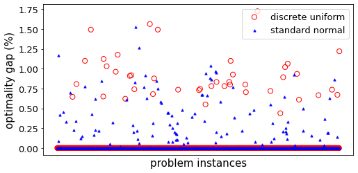
Figure 2: The plot illustrates optimality gaps for two distinct sets of QUBO problem instances, each containing one thousand instances for $n=17$ qubits. The red circles $({\color[rgb]{1,0,0}\circ})$ and blue triangles $({\color[rgb]{0,0,1}\blacktriangle})$ represent the gaps for the two sets where the $\mathsf{Q}$ matrix is sampled from the discrete uniform and standard normal distributions, respectively. The INN consistently yields the global minimum, achieving a success rate of $95\%$ and $89\%$ for the uniform and normal distributions, respectively. In both cases, the optimality gaps remain under $2\%$.

For $n=17$ qubits, to generate QUBO instances, we sampled $\mathsf{Q}$ from one of the two distributions: the uniform distribution over the set $\{-10,\cdots,10\}$ of integers and the standard normal distribution. From each distribution, we generated one thousand QUBO instances. For each instance, we obtained $E_{\text{min}}$ through an exhaustive search over $d=2^{17}=131072$ possibilities and reported the optimality gap in Fig. 2. In the case of discrete uniform distribution, we achieved the global minimum in ${958}$ out of ${1000}$ instances, meaning that the gap was $\leq 10^{-10}$. Over all the instances, the mean and maximum gaps were $0.04\%$ and $1.72\%$, respectively. When using the standard normal distribution, we reached the global minimum in ${894}$ instances, and the mean and maximum gaps were $0.04\%$ and $1.52\%,$ respectively. For each instance, we maintained a consistent configuration with a number of layers, $L=2$, and carried out $201$ epochs of training with a learning rate of $0.05$ and $\text{betas}=(0.5,0.9)$ for the Adam optimizer. Further details can be found in Arun_GitHub .

It will be interesting to see how the INN will perform if we increase the system size $n$. For this, we need quantum hardware that can store ${|\Phi\rangle}$ and return $\mathcal{E}(\Phi)$. Beyond certain $n$, classical hardware cannot store exponentially many numbers $\langle j|\Phi\rangle$ for $j=0,\cdots,2^{n}-1$. It is a true power for a quantum computer Peruzzo14 . We are not exploring this direction any further but moving to the next problem.

In a $C$-class classification problem, our goal is to predict the true label $y=(y_{1},\cdots,y_{C})\in\{0,1\}^{C}$ for a data point based on its features provided in x. When the true class is $c$, $y_{c}=1$, and the remaining components of $y$ are set to zero. During the training process of a NN for the problem, the objective is to minimize a specific loss function, such as the cross-entropy (negative log-likelihood)

$$\mathcal{L}=-\frac{1}{N}\sum_{i=1}^{N}\sum_{c=1}^{C}y^{[i]}_{c}\ln(p^{[i]}_{c})$$ (11)

within the parameter space. The outer summation in (11) is performed over a mini-batch $\{\textbf{x}^{[i]},y^{[i]}\}_{i=1}^{N}$ containing $N$ data points.

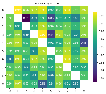
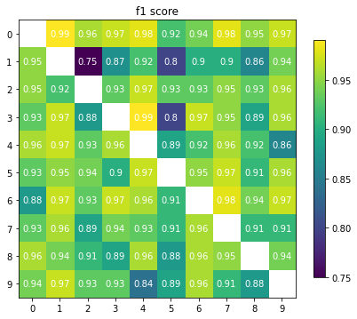
Figure 3: The top and bottom matrices display the accuracy and $\text{f}_{1}$ scores of trained INNs for binary classification problems. The entry in $a$th row and $b$th column corresponds to the image classification task of digit $a$ (negative class) against digit $b$ (positive class). It can be observed that the INN achieves accuracy ranging from $0.81$ to $0.99$ and $\text{f}_{1}$ scores between $0.75$ and $0.99$.

Suppose the dataset contains only $C=2$ classes, then one can interpret $p$ of (II) as the probability of a data point belonging to the positive class ($c=1$) and ${1-p}$ as the probability of it belonging to the negative class ($c=0$). Consequently, the INN exhibited in Fig. 1 can be employed for binary classification. To illustrate this, we have utilized the MNIST dataset MNIST , which contains images of 0 to 9 handwritten digits. To create a 2-class classification problem, we gathered all the images of only two specific digits, denoted as $a$ and $b$, which are respectively labeled as the negative class $y=(1,0)$ and the positive class $y=(0,1)$. After the training of the INN, we evaluate its performance by using

accuracy $$=\frac{\text{TP}+\text{TN}}{\text{TP}+\text{TN}+\text{FP}+\text{FN}}\quad\text{and}$$

$$\text{f}_{1} =\frac{2\,\text{TP}}{2\,\text{TP}+\text{FP}+\text{FN}}$$ (12)

on the test set. The results are presented in Fig. 3 for every $a,b\in\{0,\cdots,9\}$ provided $a\neq b$. Here, TP, TN, FP, and FN represent the counts of true positives, true negatives, false positives, and false negatives, respectively. Note that if we were to interchange the labels of $a$ and $b$, then $\mathcal{L}$, the trained INN, accuracy, and $\text{f}_{1}$ score will be different. As a result, the matrices in Fig. 3 are not symmetric around their diagonals. Various binary classifications have been carried out on the MNIST dataset in Farhi18 ; Franken20 ; Huggins19 ; Grant18 ; Schuld20 employing diverse PQCs. In our case, we achieve comparable performance, as illustrated in Fig. 3.

An image consists of $d=\mathsf{C}\times\mathsf{H}\times\mathsf{W}$ pixel values, where $\mathsf{C}$, $\mathsf{H}$, and $\mathsf{W}$ denote the number of channels, height, and width in pixels, respectively. Since the MNIST dataset contains black and white images, $\mathsf{C}=1$. To get the results of Fig. 3, we have pre-processed the data, setting $\mathsf{H}=\mathsf{W}=2^{4}$, and scaled all pixel values to the range of $-1$ to $1$. After flattening an image, we obtain a $d=2^{8}$ component feature vector x, which is then transformed into $|\textbf{x}\rangle$ following (2). Subsequently, we pass $|\textbf{x}\rangle$ through the INN shown in Fig. 1, utilizing $L=2$ layers. Other hyperparameters, including the learning rate, betas, batch size, and number of epochs, are set to $0.01$, $(0.5,0.9)$, $2^{6}$, and $10$, respectively (for additional details, refer to Arun_GitHub ). For every $(a,b)$, we maintain the same settings as described above to obtain the results presented in Fig. 3. In every case, the INN achieves an accuracy of more than $80\%$ and $\text{f}_{1}$ score more than $75\%$. These scores can potentially be further improved by modifying the INN architecture and fine-tuning the hyperparameters.

To classify images of the MNIST dataset into the $C=10$ classes, we need a NN that takes a $d_{\text{in}}$-dimensional input and provides a $d_{\text{out}}$-dimensional output, where $d_{\text{out}}$ is not necessarily the same as $d_{\text{in}}$. Let us take $d_{\text{in}}=3$, $d_{\text{out}}=2$, and compare

$$\textbf{x}^{\prime}=W\textbf{x}=\begin{pmatrix}w_{00}&w_{01}&w_{02}\\ w_{10}&w_{11}&w_{12}\\ \end{pmatrix}\begin{pmatrix}x_{0}\\ x_{1}\\ x_{2}\end{pmatrix}\quad\text{with}$$ (13)

$$FU(\bm{\phi})|\textbf{x}\rangle\equiv\frac{1}{\sqrt{3}}\begin{pmatrix}\text{e}^{\texttt{i}\phi_{0}}&\text{e}^{\texttt{i}\phi_{1}}&\text{e}^{\texttt{i}\phi_{2}}\\ \text{e}^{\texttt{i}\phi_{0}}&\text{e}^{\texttt{i}(\phi_{1}+\frac{2\pi}{3})}&\text{e}^{\texttt{i}(\phi_{2}+\frac{4\pi}{3})}\\ \text{e}^{\texttt{i}\phi_{0}}&\text{e}^{\texttt{i}(\phi_{1}+\frac{4\pi}{3})}&\text{e}^{\texttt{i}(\phi_{2}+\frac{2\pi}{3})}\end{pmatrix}\begin{pmatrix}x_{0}\\ x_{1}\\ x_{2}\end{pmatrix}.$$

The above equations represent a single linear layer of a classical NN (multi-layer perceptron) LeCun15 ; Goodfellow16 ; Aggarwal23 and a single layer of INN of Fig. 1, respectively. Here, we have used amplitude encoding (2) by assuming $\|\textbf{x}\|=1$. The linear layer combines the input features from x in a weighted manner to generate new features in $\textbf{x}^{\prime}$, while the INN layer creates interference among the input features to generate new features.

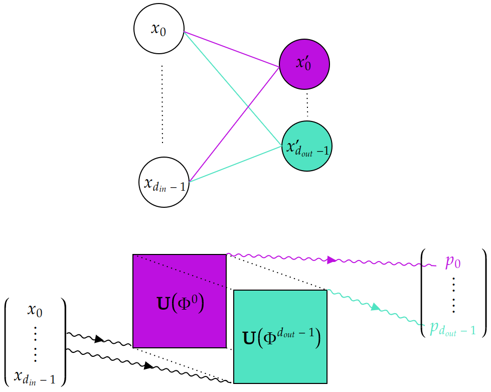
Figure 4: The top and bottom pictures exhibit a linear layer [for example, given in (13)] of a classical NN and an interferometric block [specified by (II)] of an INN, respectively. By the color coding one can see a similar parallel structure in both cases. The linear layer and INN block turn the input $\textbf{x}\in\mathbb{R}^{d_{\text{in}}}$ into the outputs $\textbf{x}^{\prime}\in\mathbb{R}^{d_{\text{out}}}$ and $\textbf{p}\in[0,1]^{\times d_{\text{out}}}$, respectively. In the bottom picture, the squares represent $d_{\text{in}}\times d_{\text{in}}$ independent unitary matrices $\textbf{U}(\Phi^{t})$, each of which is a sequence of interferometers as depicted in Fig. 1.

Two more differences can be observed through (13). Firstly, the output dimension is 2 in the case of the linear layer, while it is $3$ (not equal to the desired $d_{\text{out}}$) for the INN layer. Secondly, each row of $W$ is unrelated to the others, whereas the rows of any unitary matrix must follow the orthogonality relation. As a result, we get distinct new features $\sum_{j}w_{0j}x_{j}$ and $\sum_{j}w_{1j}x_{j}$ from the linear layer. Whereas, from the INN layer, the new features like $\sum_{j}\text{e}^{\texttt{i}\phi_{j}}x_{j}$ and $\sum_{j}\text{e}^{\texttt{i}\phi_{j}}x_{j}\,\omega^{j}$ represent very similar functions (machine learning modes) of the same set $\bm{\phi}$ of parameters, and $\omega=\text{e}^{\texttt{i}\frac{2\pi}{3}}$ is a constant. Furthermore, their derivatives with respect to a parameter only differ by a constant. So, to get $d_{\text{out}}$ distinct features, we put $d_{\text{out}}$ distinct INNs of Fig. 1 in parallel and obtain

$$|\textbf{x},\Phi^{t}\rangle =\textbf{U}(\Phi^{t})|\textbf{x}\rangle\,,\quad\mbox{where}$$

$$\textbf{U}(\Phi^{t}) =\left(\prod_{l=1}^{L}FU(\bm{\phi}^{tl})\right)F\quad\mbox{and}$$

$$p_{t} =|\langle 0|\textbf{x},\Phi^{t}\rangle|^{2}$$ (14)

for $t=0,\cdots,d_{\text{out}}-1$. Similar to how (II) represents a sequence of interferometers, (II) portrays a block of sequences of interferometers, as displayed in Fig. 4. In the figure, we also illustrate the similarity of (II) to a linear layer that represents $d_{\text{out}}$ linear regression models in parallel. One can observe that, from the same ${|\textbf{x}\rangle}$, we get $d_{\text{out}}$ distinct probabilities $p_{t}$ through $d_{\text{out}}$ mutually independent unitary operators $\textbf{U}(\Phi^{t})$, each of which represents a sequence of $L$ interferometers. Since these probabilities are independent of each other, they are not required to sum up to 1. If their normalization is needed, one can apply the function

$$\text{softmax}\,(p_{t})=\frac{\text{e}^{\,p_{t}}}{\sum_{t=0}^{d_{\text{out}}-1}\text{e}^{\,p_{t}}}$$ (15)

to every component of $\textbf{p}=(p_{0},\cdots,p_{d_{\text{out}}-1})$. Essentially, the INN block (II) creates distinct new features p from the old x through independent interferences. The vector p can serve as a final output or an input to the next INN block as shown in Fig. 5.

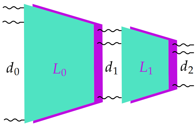
Figure 5: The diagram illustrates an INN composed of two interferometric blocks, depicted as trapezoids. Each block shares a similar structure as shown in Fig. 4. From left to right, the INN transforms the dimensions as $d_{0}\rightarrow d_{1}\rightarrow d_{2}.$ The number of layers in the first and second blocks are denoted as $L_{0}$ and $L_{1}$, respectively. The architecture of this INN is characterized by $\textbf{d}=(d_{0},d_{1},d_{2})$ and $\textbf{L}=(L_{0},L_{1})$.

Figure 5 shows an INN whose architecture is defined by $\textbf{d}=(d_{0},\cdots,d_{M-1},d_{M})$ and $\textbf{L}=(L_{0},\cdots,L_{M-1})$, where the number of blocks $M$ is 2. Its $m$th block takes $d_{m}$-dimensional input and gives $d_{m+1}$-dimensional output. Within the block, there are $d_{m+1}$ parallel sequences of interferometers represented by $\otimes_{t=0}^{d_{m+1}-1}\textbf{U}(\Phi^{t})$, and the length of each sequence is $L_{m}$.

While the INN in Fig. 5 draws inspiration from multilayer perceptrons (NNs) LeCun15 ; Goodfellow16 ; Aggarwal23 like the quantum NNs (QNNs) in Farhi18 ; Altaisky01 ; Beer20 , it differs in the following aspects. A single quantum preceptron in Altaisky01 is a sum of single-qubit unitary operators, whereas it is a product of unitary operators in the case of INN as shown in (II). Compared to Farhi18 ; Beer20 , the INN has a parallel structure of unitary operators, as depicted in Fig. 4. In contrast to the QNNs from Farhi18 ; Altaisky01 ; Beer20 , where each node represents a qubit, INNs do not necessitate a qubit system. INNs are applicable in any dimension and explicitly incorporate Fourier transformations.

Table 1: For the two datasets, we present the accuracy and average $\text{f}_{1}$ score achieved on their test sets by two separately trained INNs specified by the L values. Both the INNs have, same $\textbf{d}=(2^{8},2^{6},C)$, a $M=2$ blocks architecture as depicted in Fig. 5. Notably, as we increase the number of layers, both metrics show improvement for both datasets.

dataset	metric	$\textbf{L}=(1,1)$	$\textbf{L}=(2,2)$
MNIST	accuracy	0.89	0.93
	average $\text{f}_{1}$	0.89	0.93
FashionMNIST	accuracy	0.78	0.83
	average $\text{f}_{1}$	0.77	0.83

We have employed INNs, as illustrated in Fig. 5, for image classification on both the MNIST and FashionMNIST Xiao17 datasets, each with $C=10$ classes. The FashionMNIST dataset, like MNIST, consists of images representing clothing items from ten (labeled 0 to 9) different categories. In both cases, we have adopted $\textbf{d}=(2^{8},2^{6},C)$, the amplitude encoding of $16\times 16$ images, $0.01$ learning rate, $2^{5}$ batch size, and 3 epochs (for further details, refer to Arun_GitHub ). Their performances on the test sets are presented in Table 1 for $\textbf{L}=(1,1)$ and $(2,2)$. As we increase the number of layers, the performance—measured by the accuracy and average $\text{f}_{1}$—of the INN improves for both datasets. In summary, we have attained accuracies and average $\text{f}_{1}$ scores of ${93\%}$ and ${83\%}$ on the MNIST and FashionMNIST datasets, respectively.

The $\text{f}_{1}$ score in (II) pertains to the positive class. We can utilize a similar formula to calculate the $\text{f}_{1}$ score for each class and then derive the average $\text{f}_{1}$ score. It is also possible to extend the accuracy formula presented in (II) from $C=2$ to $C=10$ classes. In the case of the cross-entropy loss function described in (11), it is essential to ensure that the probabilities are appropriately normalized. This can be accomplished by employing the softmax function outlined in (15).

We conclude this section with the following two observations: (i) It is of interest to investigate whether the pair $\{U(\bm{\phi}),F\}$ from (II) constitutes a universal set—capable of generating any unitary operation through multiplications—for quantum computation with a $d$-level system. Notably, for $d=2$, it is a known universal set Nielsen_Chuang . Moreover, $U(\bm{\phi})$ encompasses all diagonal unitary operations and can be expressed as a linear combination of different powers of $Z=\sum_{j=0}^{d-1}\omega^{j}|j\rangle\langle j|$. Through multiplication, $Z$ and $X=F^{3}ZF$ can generate the Heisenberg-Weyl group Durt10 , whose elements constitute the unitary operator bases Schwinger60 .

(ii) As a black and white image is a two-dimensional (2D) object, instead of (2), one can use

$$|\textbf{x}\rangle_{\text{2D}}=\frac{1}{\|\textbf{x}\|}\sum_{j=0}^{\mathsf{H}-1}\sum_{j^{\prime}=0}^{\mathsf{W}-1}x_{jj^{\prime}}\,|j\rangle\otimes|j^{\prime}\rangle\,,$$ (16)

to encode an image x into two quantum subsystems with dimensions $\mathsf{H}$ and $\mathsf{W}$, where $d=1\times\mathsf{H}\times\mathsf{W}$. Then, one can use the tensor product $F_{\mathsf{H}}\otimes F_{\mathsf{W}}$ and $U(\bm{\phi})=\sum_{k}\sum_{k^{\prime}}\text{e}^{\texttt{i}\phi_{kk^{\prime}}}|k\rangle\langle k|\otimes|k^{\prime}\rangle\langle k^{\prime}|$ at the place of (II). The tensor product performs a 2D discrete Fourier transform on the matrix $x_{jj^{\prime}}$, with $F_{\mathsf{H}}$ and $F_{\mathsf{W}}$ operating exclusively on their respective subsystems. Afterward, $U(\bm{\phi})$ executes a componentwise multiplication between the phase matrix (filter) $\text{e}^{\texttt{i}\phi_{kk^{\prime}}}$ and the Fourier-transformed matrix $\widehat{x}_{kk^{\prime}}$. As per the convolution theorem, such multiplication in the frequency domain is linked to convolution in the spatial domain through Fourier transforms. Fourier transforms are fundamental components of digital image processing, particularly for designing various filters in the frequency domain Gonzalez02 .

III IGAN

In this section, we introduce IGANs, and our primary contributions are summarized as follows: Tables 2 and 3 detail the architectures and hyperparameters of IGANs, Algorithm 1 outlines the training process, and the implementation can be found in Arun_GitHub . Figure 9 offers insights into how losses and probabilities evolve during the training. And, Figs. 7 and 8 display sample images generated after the training process.

In 2014, Ian Goodfellow and colleagues introduced the generative adversarial networks (GANs) Goodfellow14 , comprising two NNs: the generator $G$ and the discriminator $D$. The generator takes random noise vectors z and endeavors to produce outputs $G(\textbf{z})$ that closely resemble real data. Meanwhile, the discriminator, acting as a binary classifier, distinguishes between real data x labeled as 1 and fake data ${G(\textbf{z})}$ labeled as 0. It assesses both real and generated data and provides a probability score for an input being real.

To enhance classification accuracy, the discriminator aims to drive $D(\textbf{x})$ closer to 1 through maximization and $D(G(\textbf{z}))$ closer to 0 through minimization. Both objectives are accomplished by minimizing the discriminator’s loss

$$\mathcal{L}_{D} =-\frac{1}{2N}\sum_{i=1}^{N}\left[\ln(D(\textbf{x}^{[i]}))+\ln(1-D(G(\textbf{z}^{[i]})))\right]\,,$$

$$\mathcal{L}_{G} =-\frac{1}{N}\sum_{i=1}^{N}\ln(D(G(\textbf{z}^{[i]})))$$ (17)

serves as a guide for the generator. It encourages the generator to produce increasingly realistic data, thereby pushing $D(G(\textbf{z}))$ closer to 1. In (III), every summation is over a mini-batch, where $\{\textbf{x}^{[i]}\}_{i=1}^{N}$ originates from the given data and $\{\textbf{z}^{[i]}\}_{i=1}^{N}$ is drawn from a prior (in our case, the standard normal) distribution.

The two networks are trained simultaneously as described in Algorithm 1 inspired from Goodfellow14 . Initially, $\mathcal{L}_{D}$ is minimized with respect to the discriminator’s parameters, followed by minimizing $\mathcal{L}_{G}$ with respect to the generator’s parameters within a single iteration (epoch). The two networks compete with each other and seek the Nash equilibrium point, where the discriminator is unable to distinguish between real and fake data. There both the probabilities $D(\textbf{x})$ and $D(G(\textbf{z}))$ attain a value of $\frac{1}{2}$, resulting in $\mathcal{L}_{D}=\ln(2)=\mathcal{L}_{G}$.

Training a GAN can be a challenging and unstable process. Therefore, several GAN variants, such as Deep Convolutional GANs Radford15 and Wasserstein GANs Arjovsky17 ; Gulrajani17 , have been developed. Deep Convolutional GANs introduced architectural guidelines for generator and discriminator networks, leading to more stable training and the generation of realistic and detailed images. Wasserstein GANs introduced the Wasserstein distance as a more stable and meaningful loss function for GAN training, effectively addressing issues like mode collapse.

Input: batch size $N$, number of epochs, learning rate, Adam hyperparameters $(\beta_{1},\beta_{2})$ from Table 3.

$\bullet$ Initialize parameters of discriminator $\bm{\Phi}_{D}$ and of generator $\bm{\Phi}_{G}$ with the Xavier initialization Glorot10 .

for number of epochs do

       for number of mini-batches do

             $\bullet$ Sample mini-batch $\{\textbf{z}^{[i]}\}_{i=1}^{N}$ from the standard normal distribution ${\mathcal{N}(0,1)}$.

            $\bullet$ Sample mini-batch $\{\textbf{x}^{[i]}\}_{i=1}^{N}$ from the training dataset.

            $\bullet$ Update $\bm{\Phi}_{D}\leftarrow\text{Adam}(\nabla_{\bm{\Phi}_{D}}\mathcal{L}_{D},\beta_{1},\beta_{2})$

            $\bullet$ Update $\bm{\Phi}_{G}\leftarrow\text{Adam}(\nabla_{\bm{\Phi}_{G}}\mathcal{L}_{G},\beta_{1},\beta_{2})$

       end for

      

end for

Algorithm 1 IGAN training algorithm

Table 2: The table presents the architecture of INNs for the discriminator $D$ and generator $G$ of separate IGANs trained on the two datasets. In both cases, every INN is of the structure depicted in Fig. 5.

dataset	INN	d	L
MNIST	$D$	$(20^{2},2^{6},1)$	$(3,3)$
	$G$	$(2^{3},2^{6},20^{2})$	$(3,3)$
CelebA	$D$	$(32^{2},2^{7},1)$	$(3,3)$
	$G$	$(2^{5},2^{7},32^{2})$	$(3,3)$

Table 3: The table presents the hyperparameters utilized in Algorithm 1 for training separate IGANs on the two datasets.

dataset	data size	batch size	epochs	rate	$(\beta_{1},\beta_{2})$
MNIST	$5000$	$2^{7}$	10	$0.01$	$(0.5,0.9)$
CelebA	$50000$	$2^{9}$	10	$0.01$	$(0.5,0.9)$

In the quantum domain, several models have been employed for image generation, including the quantum GANs Huang21 ; Tsang22 ; Zhou23 ; Stein21 ; Chu22 , Born machines Liu18 ; Benedetti19b ; Rudolph22 , matrix product states Han18 , and quantum variational autoencoder Khoshaman19 . In quantum GANs, described in Huang21 ; Tsang22 , images are created from multiple patches generated in parallel by sub-generators from a product state, which encodes the components of z into rotation angles. The loss function in Tsang22 is inspired by Wasserstein GANs Gulrajani17 . In contrast, quantum GANs in Stein21 ; Chu22 leverage quantum state fidelity-based loss functions and incorporate principal component analysis for input image compression. In the case of hybrid quantum-classical GANs discussed in Zhou23 , a specific remapping method is employed to enhance the quality of generated images. The generative models in Liu18 ; Benedetti19b ; Han18 are built using datasets of binary images. In Rudolph22 ; Benedetti18 ; Khoshaman19 , quantum models are employed for producing noise vectors z. Similar to our IGAN, the MNIST dataset is utilized in all the generative models introduced in Huang21 ; Tsang22 ; Zhou23 ; Stein21 ; Chu22 ; Han18 ; Rudolph22 ; Benedetti18 ; Khoshaman19 .

Now, we introduce our IGANs, where both the generator $G$ and discriminator $D$ are INNs as shown in Fig. 5. It is important to note that our approach does not involve principal component analysis for input compression, binary images for training, or the inclusion of any classical layers within our INNs. For input loading, we always use amplitude encoding (2) for classical vectors such as x, z, and p. An output from an interferometric block is always a classical vector p as illustrated in Fig. 4. From the generator, we get $\textbf{p}\in[0,1]^{\times d}$ with an image size of $d=\mathsf{C}\times\mathsf{H}\times\mathsf{W}$, which, after the componentwise transformation

$$\textbf{p}\rightarrow\tanh(2\,\textbf{p}-1)=G(\textbf{z})\in[-1,1]^{\times d}\,,$$ (18)

is fed to the discriminator during training. The discriminator’s output, $D(\textbf{x})$ or $D(G(\textbf{z}))$, represents the probability, $p\in[0,1]$, of the input being real, where the corresponding $\textbf{p}=(1-p\,,p)$. The training process for our IGANs is outlined in Algorithm 1 and its complete implementation is given in Arun_GitHub .

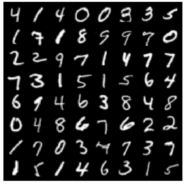
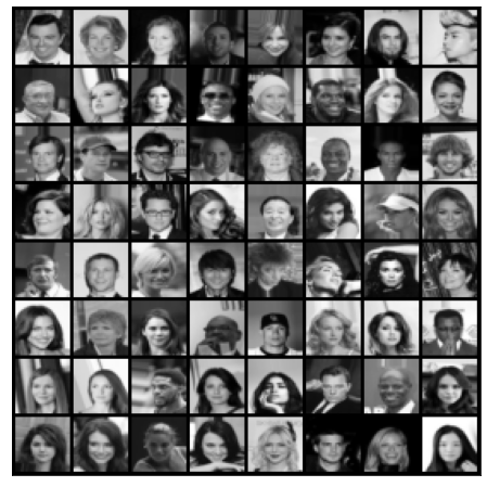
Figure 6: The top and bottom panels showcase samples of 64 real images from the MNIST MNIST and CelebA CelebA datasets, respectively.

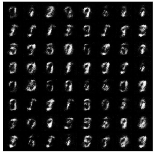
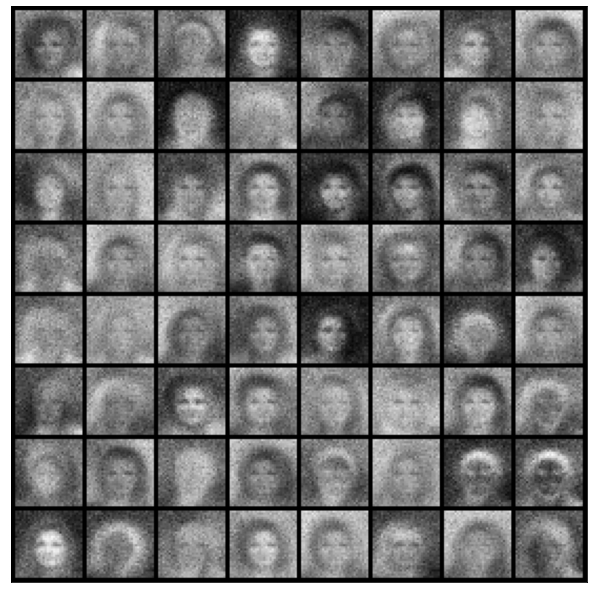
Figure 7: After separately training IGANs on the MNIST MNIST and CelebA CelebA datasets, the top and bottom panels showcase 64 fake images generated by their respective generators. To enhance contrast, we have employed the transformation $\textbf{p}\rightarrow\tanh(3(2\,\textbf{p}-1))$ at the place of (18) exclusively for image generation in the top panel and Fig. 8.

Separate IGANs were trained on the MNIST dataset MNIST and CelebA datasets CelebA , which consists of images featuring celebrities’ faces as displayed in Fig. 6. Subsequently, samples of generated images from their respective $G$s are presented in Fig. 7. In both cases, black and white images were used for training, and 2-block INNs were employed for both $D$ and $G$. For the two datasets, we have adopted slightly different architectures for the INNs, as detailed in Table 2, and slightly varied hyperparameters, as specified in Table 3.

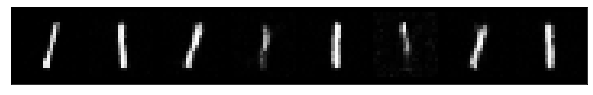
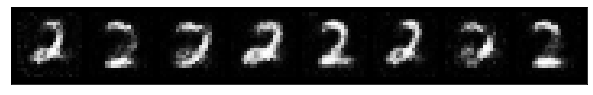
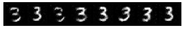
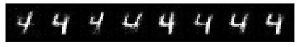
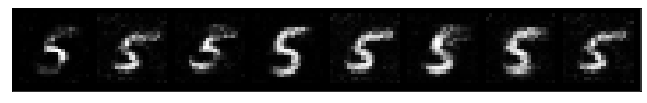
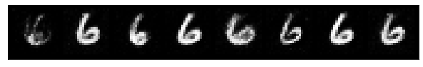
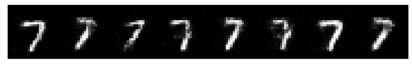
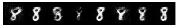
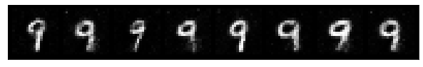
Figure 8: From top to bottom, each row displays eight fake images generated by the $G$ network trained separately on real images of digits $0,\cdots,9$. For each digit, we maintained consistent architecture and hyperparameters (with the exception of data size) as those presented in Tables 2 and 3 for the MNIST dataset. The training data was sourced from the MNIST training set.

In the case of the MNIST dataset, we have randomly taken 5000 images of 0 to 9 digits for the training as specified in the “data size” column of Table 3. Each image has dimensions $d=\mathsf{C}\times\mathsf{H}\times\mathsf{W}=1\times 20\times 20$, as evident from the first and last components of ds for $D$ and $G$ in Table 2. In the top panel of generated images in Fig. 7, clear representations of numbers 0, 1, 3, 5, and 9 are easily noticeable. However, the images of 2, 4, and 6 appear less distinct, while those of 7 and 8 do not seem to be present. In another set of experiments, we trained the same IGAN using images of a single digit at a time and achieved the results depicted in Fig. 8. These results demonstrate our capability to generate images corresponding to all ten digits, from 0 to 9. One can visually assess the quality of generated images by comparing them to real images through Figs. 6–8.

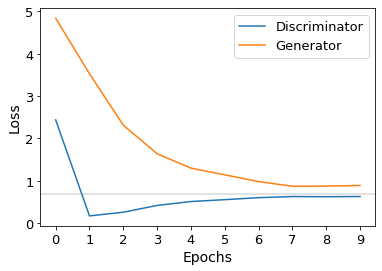
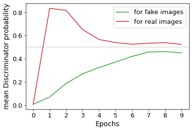
Figure 9: At the top, we present the evolution of $\mathcal{L}_{D}$ and $\mathcal{L}_{G}$ at various epochs, represented by orange and blue curves, respectively. Meanwhile, at the bottom, we illustrate the changes in $\mathcal{P}_{\text{real}}$ and $\mathcal{P}_{\text{fake}}$ over different epochs, denoted by red and green graphs, respectively. The definitions of these loss functions and average probabilities can be found in (III) and (19), respectively. In the top and bottom plots, the gray horizontal lines denote the values $\ln(2)$ and $\frac{1}{2}$, respectively. Both the plots pertain to the IGAN trained on the CelebA dataset.

In the case of the CelebA dataset, we randomly selected 50000 images for training. These images were converted from color to black and white and resized to the dimensions of $d=1\times 32\times 32$, as detailed in Table 2. With the table, one can also compute that the INNs for $D$ and $G$ have a total of 393600 and 405504 trainable parameters (phases), respectively. In Fig. 9, we depict how the discriminator and generator losses converge toward $\ln(2)$ as training progresses. Additionally, we illustrate how the average discriminator probabilities

$$\mathcal{P}_{\text{real}}=\frac{1}{N}\sum_{i=1}^{N}D(\textbf{x}^{[i]})\quad\mbox{and}\quad\mathcal{P}_{\text{fake}}=\frac{1}{N}\sum_{i=1}^{N}D(G(\textbf{z}^{[i]}))$$ (19)

approach $\tfrac{1}{2}$. After the training, we got the ability to generate images featuring human faces, as showcased in Fig. (7). By the way, with the average probabilities, one can define $\mathcal{L}^{\prime}_{D}=-\mathcal{P}_{\text{real}}+\mathcal{P}_{\text{fake}}$ and $\mathcal{L}^{\prime}_{G}=-\mathcal{P}_{\text{fake}}$, inspired from the Wasserstein loss functions Arjovsky17 ; Gulrajani17 ; Tsang22 , at place of (III).

IV conclusion and outlook

We have introduced INNs, which are artificial neural networks composed of interferometers. An INN is a sequence of interferometric blocks, with each block containing parallel sequences of interferometers. While one could, in principle, use an INN with classical waves, it can be regarded as a quantum model, devoid of any classical layers.

We have shown that INNs are useful for optimization as well as supervised or unsupervised machine learning tasks. For the QUBO problems, we achieve the global minimum approximately ${90\%}$ of the time, with the remaining instances typically falling within a range of ${2\%}$ from the global minimum. In the context of multi-class image classification problems, we achieved accuracies of ${93\%}$ and ${83\%}$ on the MNIST and FashionMNIST datasets, respectively. While our accuracy falls short in comparison to state-of-the-art classical NNs, which provide ${99.87\%}$ accuracy on the MNIST dataset Byerly20 , and ${96.91\%}$ accuracy on the FashionMNIST dataset Tanveer20 , it is important to note that INNs exhibit a simpler architecture. Nonetheless, our work represents a significant step forward in the development of more advanced quantum NNs.

We have introduced IGANs, made of INNs, for image generation. These IGANs have successfully generated images of 0 to 9 digits and human faces. While our image quality may currently lag behind that of classical GANs Goodfellow14 ; Radford15 ; Arjovsky17 ; Gulrajani17 , there is potential for enhancement through network modifications, architectural adjustments, and fine-tuning of hyperparameters. Last but not least, it is crucial to analyze the robustness of our INNs against noise and qubit errors, which will be the focus of future research.

References

- (1) Y. LeCun, Y. Bengio, and G. Hinton, Nature 521, 436 (2015).
- (2) I. Goodfellow, Y. Bengio, and A. Courville, Deep Learning (MIT Press, 2016).
- (3) C. C. Aggarwal, Neural Networks and Deep Learning : A Textbook (Springer Nature Switzerland AG, 2023).
- (4) Y. LeCun, B. Boser, J. S. Denker, D. Henderson, R. E. Howard, W. Hubbard, and L. D. Jackel, Neural Comput. 1, 541 (1989).
- (5) Y. Lecun, L. Bottou, Y. Bengio, and P. Haffner, Proc. IEEE 86, 2278 (1998).
- (6) A. Krizhevsky, I. Sutskever, and G. E. Hinton, in Proc. Advances in Neural Information Processing Systems 25, 1090 (2012).
- (7) I. J. Goodfellow, J. Pouget-Abadie, M. Mirza, B. Xu, D. Warde-Farley, S. Ozair, A. Courville, and Y. Bengio, in Proceedings of the 27th International Conference on Neural Information Processing Systems (MIT Press, 2014), Vol. 2, pp. 2672–2680.
- (8) A. Radford, L. Metz, and S. Chintala, arXiv:1511.06434 [cs.LG] (2015).
- (9) M. Arjovsky, S. Chintala, and L. Bottou, in Proceedings of the 34th International Conference on Machine Learning, PMLR 70, 214 (2017).
- (10) I. Gulrajani, F. Ahmed, M. Arjovsky, V. Dumoulin, and A. Courville, in Proceedings of the 31st International Conference on Neural Information Processing Systems 2017, pp. 5769–5779.
- (11) R. P. Feynman, R. B. Leighton, and M. Sands, The Feynman Lectures on Physics (Addison-Wesley, 1964) Vol. 3.
- (12) W. K. Wootters and W. H. Zurek, Phys. Rev. D 19, 473 (1979).
- (13) D. M. Greenberger and A. Yasin, Phys. Lett. A 128, 391 (1988).
- (14) B.-G. Englert, Phys. Rev. Lett. 77, 2154 (1996).
- (15) S. Dürr, T. Nonn, and G. Rempe, Nature 395, 33 (1998).
- (16) S. Dürr, T. Nonn, and G. Rempe, Phys. Rev. Lett. 81, 5705 (1998).
- (17) B.-G. Englert, D. Kaszlikowski, L. C. Kwek, and W. H. Chee, Int. J. Quantum Inf. 6, 129 (2008).
- (18) P. J. Coles, Phys. Rev. A 93, 062111 (2016).
- (19) T. Qureshi and M. A. Siddiqui, Ann. Phys. 385, 598 (2017).
- (20) G. Weihs, M. Reck, H. Weinfurter, and A. Zeilinger, Opt. Lett. 21, 302 (1996).
- (21) Peter W. Shor, SIAM J. Comput. 26, 1484 (1997).
- (22) M. Benedetti, E. Lloyd, S. Sack, and M. Fiorentini, Quantum Sci. Technol. 4, 043001 (2019).
- (23) A. Peruzzo, J. McClean, P. Shadbolt, M.-H. Yung, X.-Q. Zhou, P. J. Love, A. Aspuru-Guzik, and J. L. O’Brien, Nat. Commun. 5, 4213 (2014).
- (24) J. R. McClean, J. Romero, R. Babbush, and A. Aspuru-Guzik, New J. Phys. 18, 023023 (2016).
- (25) P. J. J. O’Malley et al., Phys. Rev. X 6, 031007 (2016).
- (26) M. Motta, E. Ye, J. R. McClean, Z. Li, A. J. Minnich, R. Babbush, and G. K.-L. Chan, npj Quantum Inf. 7, 83 (2021).
- (27) J. Lee, W. J. Huggins, M. Head-Gordon, and K. B. Whaley, J. Chem. Theory Comput. 15, 311 (2019).
- (28) Y. Matsuzawa and Y. Kurashige, J. Chem. Theory Comput. 16, 944 (2020).
- (29) E. Farhi, J. Goldstone, and S. Gutmann, arXiv:1411.4028 [quant-ph] (2014).
- (30) A. Lucas, Front. Phys. 2, 5 (2014).
- (31) J. Preskill, Quantum 2, 79 (2018).
- (32) O. Higgott, D. Wang, and S. Brierley, Quantum 3, 156 (2019).
- (33) K. M. Nakanishi, K. Mitarai, and K. Fujii, Phys. Rev. Research 1, 033062 (2019).
- (34) Y. Li and S. C. Benjamin, Phys. Rev. X 7, 021050 (2017).
- (35) X. Yuan, S. Endo, Q. Zhao, Y. Li, and S. C. Benjamin, Quantum 3, 191 (2019).
- (36) I. D Kivlichan, J. McClean, N. Wiebe, C. Gidney, A. Aspuru-Guzik, G. K.-L. Chan, and R. Babbush, Phys. Rev. Lett. 120, 110501 (2018).
- (37) C. Cîrstoiu, Z. Holmes, J. Iosue, L. Cincio, P. J. Coles, and A. Sornborger, npj Quantum Inf. 6, 82 (2020).
- (38) J. Gibbs, K. Gili, Z. Holmes, B. Commeau, A. Arrasmith, L. Cincio, P. J. Coles, and A. Sornborger, arXiv:2102.04313 [quant-ph] (2021).
- (39) C. Bravo-Prieto, R. LaRose, M. Cerezo, Y. Subasi, L. Cincio, and P. J Coles, arXiv:1909.05820 [quant-ph] (2019).
- (40) H.-Y. Huang, K. Bharti, and P. Rebentrost, arXiv:1909.07344 [quant-ph] (2019).
- (41) X. Xu, J. Sun, S. Endo, Y. Li, S. C. Benjamin, and X. Yuan, Sci. Bull. 66, 2181 (2021).
- (42) M. Lubasch, J. Joo, P. Moinier, M. Kiffner, and D. Jaksch, Phys. Rev. A 101, 010301(R) (2020).
- (43) O. Kyriienko, A. E. Paine, and V. E. Elfving, Phys. Rev. A 103, 052416 (2021).
- (44) E. Farhi and H. Neven, arXiv:1802.06002 [quant-ph] (2018).
- (45) W. Huggins, P. Patil, B. Mitchell, K. B. Whaley, and E. M. Stoudenmire, Quantum Sci. Technol. 4, 024001 (2019).
- (46) E. Grant, M. Benedetti, S. Cao, A. Hallam, J. Lockhart, V. Stojevic, A. G. Green, and S. Severini, npj Quantum Inf. 4, 65 (2018).
- (47) K. Mitarai, M. Negoro, M. Kitagawa, and K. Fujii, Phys. Rev. A 98, 032309 (2018).
- (48) V. Havlíček, A. D. Córcoles, K. Temme, A. W. Harrow, A. Kandala, J. M. Chow, and J. M. Gambetta, Nature 567, 209 (2019).
- (49) L. Franken and B. Georgiev, Explorations in quantum neural networks with intermediate measurements, in Proceedings of ESANN (2020).
- (50) M. Schuld and N. Killoran, Phys. Rev. Lett. 122, 040504 (2019).
- (51) M. Schuld, A. Bocharov, K. M. Svore, and N. Wiebe, Phys. Rev. A 101, 032308 (2020).
- (52) J. Romero, J. P. Olson, and A. Aspuru-Guzik, Quantum Sci. Technol. 2, 045001 (2017).
- (53) S. Lloyd and C. Weedbrook, Phys. Rev. Lett. 121, 040502 (2018).
- (54) P.-L. Dallaire-Demers and N. Killoran, Phys. Rev. A 98, 012324 (2018).
- (55) C. Zoufal, A. Lucchi, and S. Woerner, npj Quantum Inf. 5, 103 (2019).
- (56) J. Romero and A. Aspuru-Guzik, arXiv:1901.00848 [quant-ph] (2019).
- (57) M. Y. Niu, A. Zlokapa, M. Broughton, S. Boixo, M. Mohseni, V. Smelyanskyi, and H. Neven, arXiv:2105.00080 [quant-ph] (2021).
- (58) H.-L. Huang, Y. Du, M. Gong, Y. Zhao, Y. Wu, C. Wang, S. Li, F. Liang, J. Lin, Y. Xu, R. Yang, T. Liu, M.-H. Hsieh, H. Deng, H. Rong, C.-Z. Peng, C.-Y. Lu, Y.-A. Chen, D. Tao, X. Zhu, and J.-W. Pan, Phys. Rev. Applied 16, 024051 (2021).
- (59) S. L. Tsang, M. T. West, S. M. Erfani, and M. Usman, arXiv:2212.11614 [quant-ph] (2022).
- (60) N.-R. Zhou, T.-F. Zhang, X.-W. Xie, and J.-Y. Wu, Signal Process. Image Commun. 110, 116891 (2023).
- (61) S. A. Stein, B. Baheri, D. Chen, Y. Mao, Q. Guan, A. Li, B. Fang, and S. Xu, in 2021 IEEE Int. Conf. on Quantum Comput. and Eng. (Broomfield, CO, USA, 2021), pp. 71–81.
- (62) C. Chu, G Skipper, M. Swany, and F. Chen, arXiv:2210.16857 [quant-ph] (2022).
- (63) J.-G. Liu and L. Wang, Phys. Rev. A 98, 062324 (2018).
- (64) M. Benedetti, D. Garcia-Pintos, O. Perdomo, V. Leyton-Ortega, Y. Nam, and A. Perdomo-Ortiz, npj Quantum Inf. 5, 45 (2019).
- (65) B. Coyle, D. Mills, V. Danos, and E. Kashefi, npj Quantum Inf. 6, 60 (2020).
- (66) M. S. Rudolph, N. B. Toussaint, A. Katabarwa, S. Johri, B. Peropadre, and A. Perdomo-Ortiz, Phys. Rev. X 12, 031010 (2022).
- (67) J. Tian, X. Sun, Y. Du, S. Zhao, Q. Liu, K. Zhang, W. Yi, W. Huang, C. Wang, X. Wu, M.-H. Hsieh, T. Liu, W. Yang, and D. Tao, arXiv:2206.03066 [quant-ph] (2022).
- (68) M. Cerezo, A. Arrasmith, R. Babbush, S. C. Benjamin, S. Endo, K. Fujii, J. R. McClean, K. Mitarai, X. Yuan, L. Cincio, and P. J. Coles, Nat. Rev. Phys. 3, 625 (2021).
- (69) K. Bharti, A. Cervera-Lierta, T. H. Kyaw, T. Haug, S. Alperin-Lea, A. Anand, M. Degroote, H. Heimonen, J. S. Kottmann, T. Menke, W.-K. Mok, S. Sim, L.-C. Kwek, and A. Aspuru-Guzik, Rev. Mod. Phys. 94, 015004 (2022).
- (70) https://github.com/ArunSehrawat/Interferometric-Neural-Networks
- (71) A. Paszke, S. Gross, F. Massa, A. Lerer, J. Bradbury, G. Chanan, T. Killeen, Z. Lin, N. Gimelshein, L. Antiga, A. Desmaison, A. Köpf, E. Yang, Z. DeVito, M. Raison, A. Tejani, S. Chilamkurthy, B. Steiner, L. Fang, J. Bai, and S. Chintala, arXiv:1912.01703 [cs.LG] (2019).
- (72) D. P. Kingma and J. Ba, arXiv:1412.6980 [cs.LG] (2014).
- (73) L. K. Grover, Phys. Rev. Lett. 79, 325 (1997).
- (74) Y. LeCun, C. Cortes, and C. J. Burges, The MNIST Database of Handwritten Digits, [Online] Available: http://yann.lecun.com/exdb/mnist/
- (75) M. V. Altaisky, arXiv:quant-ph/0107012 (2001).
- (76) K. Beer, D. Bondarenko, T. Farrelly, T. J. Osborne, R. Salzmann, D. Scheiermann, and R. Wolf, Nat. Commun. 11, 808 (2020).
- (77) H. Xiao, K. Rasul, and R. Vollgraf, arXiv:1708.07747 [cs.LG] (2017).
- (78) M. A. Nielsen and I. L. Chuang, Quantum Computation and Quantum Information (Cambridge University Press, 2010), Chapter 4.
- (79) T. Durt, B.-G. Englert, I. Bengtsson, and K. Życzkowski, Int. J. Quantum Inf. 8, 535 (2010).
- (80) J. Schwinger, Proc. Natl. Acad. Sci. U. S. A. 46, 570 (1960).
- (81) R. C. Gonzalez and R. E. Woods, Digital Image Processing, (Prentice-Hall, 2002).
- (82) X. Glorot and Y. Bengio, in Proceedings of the Thirteenth International Conference on Artificial Intelligence and Statistics, PMLR 9, 2010, pp. 249–256.
- (83) Z.-Y. Han, J. Wang, H. Fan, L. Wang, and P. Zhang, Phys. Rev. X 8, 031012 (2018).
- (84) A. Khoshaman, W. Vinci, B. Denis, E. Andriyash, H. Sadeghi, and M. H. Amin, Quantum Sci. Technol. 4, 014001 (2019).
- (85) M. Benedetti, J. Realpe-Gómez, and A. Perdomo-Ortiz, Quantum Sci. Technol. 3, 034007 (2018).
- (86) Z. Liu, P. Luo, X. Wang, and X. Tang, in 2015 IEEE International Conference on Computer Vision (ICCV), 2015, pp. 3730–3738.
- (87) A. Byerly, T. Kalganova, and I. Dear, arXiv:2001.09136 [cs.CV] (2020).
- (88) M. S. Tanveer, M. U. K. Khan, and C.-M. Kyung, arXiv:2006.09042 [cs.CV] (2020).