Harmonic model predictive control for tracking periodic references

Abstract

Harmonic model predictive control (HMPC) is a recent model predictive control (MPC) formulation for tracking piece-wise constant references that includes a parameterized artificial harmonic reference as a decision variable, resulting in an increased performance and domain of attraction with respect to other MPC formulations. This article presents an extension of the HMPC formulation to track periodic harmonic references and discusses its use to track arbitrary references. The proposed formulation inherits the benefits of its predecessor, namely its good performance and large domain of attraction when using small prediction horizons, and that the complexity of its optimization problem does not depend on the period of the periodic reference. We show closed-loop results discussing its performance and comparing it to other MPC formulations.

I Introduction

The use of model predictive control (MPC) [1, 2] to control periodic references is a widely studied problem in the control literature since it has many practical applications, such as repetitive control [3], control of periodic systems [4, 5, 6], or economic MPC [7].

In [8], an MPC for tracking periodic references was presented as an extension of the tracking MPC formulation for piece-wise affine references from [9]. This formulation makes use of an artificial periodic reference trajectory, which becomes part of the optimization problem, whose period coincides with that of the reference. The benefits of using this artificial reference are that the resulting MPC controller is recursively feasible even in the event of a reference change, and that the closed-loop system converges to the periodic trajectory that is “closest” to the periodic reference, where the distance is measured by the terminal cost of the MPC controller. Thus, the formulation inherently deals with references that cannot be perfectly tracked. Additionally, the use of the artificial reference results in a domain of attraction that is typically significantly larger than the ones obtained from classical MPC formulations [10]. The issue, however, is that the number of decision variables of the artificial periodic reference grows with its period.

In [11], an MPC formulation heavily inspired by [9] was presented. This formulation, named harmonic model predictive control (HMPC), also tracks piece-wise constant references by including an artificial reference in the optimization problem. The difference, however, is that the artificial reference is in the form of a harmonic signal, instead of the constant one used in [9]. The authors show that this modification may lead to a significantly larger domain of attraction and performance when working with small prediction horizons, which is a desirable property for its implementation in embedded systems, where the use of a small prediction horizon is desirable to reduce the computational and memory requirements of the controller. The downside of the formulation is that the use of a harmonic artificial reference comes at the cost of the inclusion of second-order cone constraints, resulting in an optimization problem which is no longer a quadratic programming (QP) problem. However, in [12] the authors presented an efficient solver for the HMPC formulation, showing that its solution-time is comparable to state-of-the-art QP solvers applied to alternative MPC formulations.

In this paper, we present an extension of HMPC for tracking harmonic references, instead of the piece-wise constant references considered in [11]. This is a natural extension, given the fact that the HMPC formulation uses a harmonic artificial reference. The benefit of the formulation is that the complexity of the optimization problem does not depend on the period of the reference, thus being applicable to arbitrarily long periodic references. The formulation also inherently deals with non-admissible references, resulting in a closed-loop behavior which may differ from the typical one obtained from other periodic MPC formulations due to the terminal ingredients partly measuring the “distance” to the reference in terms of it “shape”, as we show in the numerical case study. This may be useful in various applications, such as power electronics or spacecraft rendezvous [4, 13]. The optimization problem of the proposed extension can be solved using a very minor modification of the solver from [12], which is available in [14]. Additionally, the proposed formulation retains the recursive feasibility and asymptotic stability of the original HMPC as well as its main benefits, namely its increased performance and domain of attraction when using small prediction horizons and the fact that the complexity of its optimization problem does not depend on the period of the periodic reference. Finally, we discuss the application of the proposed formulation to track arbitrary references, i.e., not necessarily harmonic, showing that a proper selection of the ingredients of the controller can lead to a good tracking performance, even when the complete reference signal is not known before-hand.

Notation

Given two vectors $x$ and $y$, $x\leq(\geq)\;y$ denotes componentwise inequalities. Given two integers $i$ and $j$ with ${j\geq i}$, $\mathbb{Z}_{i}^{j}$ denotes the set of integer numbers from $i$ to $j$, i.e. ${\mathbb{Z}_{i}^{j}\doteq\{i,i+1,\dots,j-1,j\}}$. We denote by $\mathbb{S}_{+}^{n}$ ($\mathbb{D}_{+}^{n}$) the set of (diagonal) positive definite matrices in $\mathbb{R}^{n\times n}$. For vectors $x_{1}$ to $x_{N}$, $(x_{1},x_{2},\dots,x_{N})$ denotes the column vector formed by their concatenation. Given a vector $x\in\mathbb{R}^{n}$, we denote its $i$-th component using a parenthesized subindex $x_{(i)}$. Given two vectors $x\in\mathbb{R}^{n}$ and $y\in\mathbb{R}^{n}$, their standard inner product is denoted by $\langle x,y\rangle\doteq\sum_{i=1}^{n}x_{(i)}y_{(i)}$. For $x\in\mathbb{R}^{n}$ and $A\in\mathbb{S}_{+}^{n}$, $\|x\|\doteq\sqrt{\langle x,x\rangle}$ and $\|x\|_{A}\doteq\sqrt{\langle x,Ax\rangle}$. The identity matrix of dimension $n$ is denoted by $I_{n}$. Given scalars and/or matrices $M_{1},M_{2},\dots,M_{N}$ (not necessarily of the same dimensions), we denote by $\texttt{diag}(M_{1},M_{2},\dots,M_{N})$ the block diagonal matrix formed by the concatenation of $M_{1}$ to $M_{N}$.

II Admissible harmonic signals

Definition 1 (Harmonic signal).

A trajectory $v(t)\in\mathbb{R}^{m}$ is a harmonic signal if it satisfies

$$v(t)=v_{e}+v_{s}\sin(wt)+v_{c}\cos(wt),\\$$ (1)

for some parameters $v_{e},v_{s},v_{c}\in\mathbb{R}^{m}$ and frequency $w>0$.

Consider a system described by a controllable linear time-invariant state-space model

$$x(t+1)=Ax(t)+Bu(t),$$ (2)

where $x(t)\in\mathbb{R}^{n_{x}}$ and $u(t)\in\mathbb{R}^{n_{u}}$ are the state and control input at the discrete time instant $t$, respectively, subject to

$$\underline{y}\leq Ex(t)+Fu(t)\leq\overline{y},$$ (3)

where we assume that the bounds $\underline{y},\overline{y}\in\mathbb{R}^{n_{y}}$ satisfy $\underline{y}<\overline{y}$.

Definition 2 (Admissible harmonic signals).

The harmonic signals $\hat{x}(t)$ and $\hat{u}(t)$ with frequency $w>0$, parametrized by ${\rm\bf{\hat{x}}}\doteq(\hat{x}_{e},\hat{x}_{s},\hat{x}_{c})$ and ${\rm\bf{\hat{u}}}\doteq(\hat{u}_{e},\hat{u}_{s},\hat{u}_{c})$, are admissible if they satisfy ${\hat{x}(t+1)}=A\hat{x}(t)+B\hat{u}(t)$ and $\underline{y}\leq E\hat{x}(t)+F\hat{u}(t)\leq\overline{y}$, $\forall t$, where if the inequalities are strictly satisfied $\forall t$ we say that they are strictly admissible.

The following propositions provide sufficient conditions for admissibility of the harmonic signal $(\hat{x}(t),\hat{u}(t))$, where we use the following notation for clarity of presentation:

$$\hat{y}_{e}\doteq E\hat{x}_{e}+F\hat{u}_{e},\;\hat{y}_{s}\doteq E\hat{x}_{s}+F\hat{u}_{s},\;\hat{y}_{c}\doteq E\hat{x}_{c}+F\hat{u}_{c}.$$

Proposition 1.

Let $\hat{x}(t)$ and $\hat{u}(t)$ be harmonic signals with the same frequency $w$ parametrized by ${\rm\bf{\hat{x}}}\doteq(\hat{x}_{e},\hat{x}_{s},\hat{x}_{c})$ and ${\rm\bf{\hat{u}}}\doteq(\hat{u}_{e},\hat{u}_{s},\hat{u}_{c})$, and

$${\mathcal{D}}\doteq\left\{({\rm\bf{\hat{x}}},{\rm\bf{\hat{u}}}):\begin{array}[]{@{}l@{}}\hat{x}_{e}=A\hat{x}_{e}+B\hat{u}_{e}\\ \hat{x}_{s}\cos(w)-\hat{x}_{c}\sin(w)=A\hat{x}_{s}+B\hat{u}_{s}\\ \hat{x}_{s}\sin(w)+\hat{x}_{c}\cos(w)=A\hat{x}_{c}+B\hat{u}_{c}\end{array}\right\}.$$

Then, $({\rm\bf{\hat{x}}},{\rm\bf{\hat{u}}})\in{\mathcal{D}}$ implies $\hat{x}(t+1)=A\hat{x}(t)+B\hat{u}(t)$, $\forall t$.

Proof.

The proposition follows from [11, Property 2]. ∎

Proposition 2.

Let $\hat{x}(t)$ and $\hat{u}(t)$ be harmonic signals with the same frequency $w$ parametrized by ${\rm\bf{\hat{x}}}\doteq(\hat{x}_{e},\hat{x}_{s},\hat{x}_{c})$ and ${\rm\bf{\hat{u}}}\doteq(\hat{u}_{e},\hat{u}_{s},\hat{u}_{c})$, and

$${\mathcal{C}}_{\sigma}\doteq\left\{(\hat{x},\hat{u}):\begin{array}[]{@{}l@{}}(\hat{y}_{e(i)},\hat{y}_{s(i)},\hat{y}_{c(i)})\in\overline{{\mathcal{Y}}}_{i}\cap\underline{{\mathcal{Y}}}_{i},\,i\in\mathbb{Z}_{1}^{n_{y}}\end{array}\right\},$$

where sets $\overline{{\mathcal{Y}}}_{i}$ and $\underline{{\mathcal{Y}}}_{i}$ are defined as

$${}\mkern-4.0mu\overline{{\mathcal{Y}}}_{i} =\left\{y=(y_{0},y_{1})\in\mathbb{R}\times\mathbb{R}^{2}:\|y_{1}\|\leq\overline{y}_{(i)}-\sigma-y_{0}\right\},$$

$${}\mkern-4.0mu\underline{{\mathcal{Y}}}_{i} =\left\{y=(y_{0},y_{1})\in\mathbb{R}\times\mathbb{R}^{2}:\|y_{1}\|\leq y_{0}-\underline{y}_{(i)}-\sigma\right\},$$

and $\sigma\geq 0$. Then, $({\rm\bf{\hat{x}}},{\rm\bf{\hat{u}}})\in{\mathcal{C}}_{\sigma}$ implies that $\hat{x}(t)$ and $\hat{u}(t)$ satisfy $\underline{y}\leq E\hat{x}(t)+F\hat{u}(t)\leq\overline{y}$, $\forall t$, where the implication follows with strict inequality if $\sigma>0$.

Proof.

The proposition follows from [11, Property 3]. ∎

Corollary 1.

A harmonic signal $(\hat{x}(t),\hat{u}(t))$ satisfying the conditions of Propositions 1 and 2 is an admissible harmonic signal of system (2) subject to (3). Furthermore, it is a strict admissible harmonic signal if the conditions of Proposition 2 are satisfied for some $\sigma>0$.

The key point of Propositions 1 and 2 is that they provide conditions for admissibility of the harmonic signal $(\hat{x}(t),\hat{u}(t))$ that only depend on the parameters ${\rm\bf{\hat{x}}}$ and ${\rm\bf{\hat{u}}}$, but not on their frequency $w$. Satisfaction of the state dynamics is guaranteed by the satisfaction of the linear constraints in ${\mathcal{D}}$, whereas satisfaction of the system constraints is guaranteed by the satisfaction of the second order cone constraints defined by sets $\overline{{\mathcal{Y}}}_{i}$ and $\underline{{\mathcal{Y}}}_{i}$.

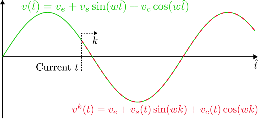
Figure 1: Harmonic signal expressed in the relative time $k$.

In the following, we will be interested in expressing harmonic signals in terms of a relative time $k$ with respect to the current time $t$. That is, for a fixed time $t$, we want to obtain an expression (1) for $v^{k}(t)\doteq v(t+k)\in\mathbb{R}^{m}$ in the form

$$v^{k}(t)=v_{e}(t)+v_{s}(t)\sin(wk)+v_{c}(t)\cos(wk)$$ (4)

for some time-varying parameters $v_{e}(t),v_{s}(t),v_{c}(t)\in\mathbb{R}^{m}$. Expression (4) is simply a time-shift of the underlying harmonic signal $v(t)$, as illustrated in Figure 1, where the current time $t$ is taken as the “initial time” of the periodic signal $v^{k}(t)$, i.e., $v^{0}(t)=v(t)$. At each time $t$, the parameters ${\rm\bf{v}}(t)\doteq(v_{e}(t),v_{s}(t),v_{c}(t))$ of (4) are obtained from the recursion $v_{e}(0)=v_{e}$, $v_{s}(0)=v_{s}$, $v_{c}(0)=v_{c}$,

$${\rm\bf{v}}(t+1)=\mathcal{T}_{h}^{m}{\rm\bf{v}}(t),\,\forall t\geq 0,$$ (5)

where $\mathcal{T}_{h}^{m}\doteq\mathtt{diag}(I_{m},\mathcal{T}_{w}^{m})$ and

$$\mathcal{T}_{w}^{m}\doteq\begin{bmatrix}I_{m}\cos(w)&-I_{m}\sin(w)\\ I_{m}\sin(w)&I_{m}\cos(w)\end{bmatrix}\in\mathbb{R}^{2m\times 2m}$$ (6)

is an orthogonal matrix. We do not provide a proof of (5), since it is a standard result (c.f., [11, Property 1]).

Henceforth, we will distinguish between trajectories and sequences: we will refer to a time-series $v(t)$ evolving in the discrete time $t$ as a trajectory, and we will use the term sequence to refer to its related signal $\{v^{k}(t)\}$ evolving in the relative time $k$ with respect to some fixed $t$, where we may drop the $(t)$ from the notation and simply write $v^{k}$ if the value of $t$ is clear from the context.

III HMPC for harmonic reference tracking

The idea behind HMPC [11] is to introduce an artificial harmonic reference in the optimization problem whose discrepancy with the desired reference is penalized in the objective function. Additionally, the objective function penalizes the discrepancy between the predicted system trajectory and this artificial reference, as is typical in MPC. In [11], HMPC was used to track set-point references, i.e., piecewise affine references $(x_{r},u_{r})\in\mathbb{R}^{n_{x}}\times\mathbb{R}^{n_{u}}$. In this article, however, the control objective is to track a harmonic reference trajectory $(x_{r}(t),u_{r}(t))$, instead of a piecewise constant reference. At each sample time $t$, this reference trajectory can be expressed by its relative-time signals

$$x_{r}^{k}(t) =x_{re}+x_{rs}(t)\sin(wk)+x_{rc}(t)\cos(wk),$$ (7a)

$$u_{r}^{k}(t) =u_{re}+u_{rs}(t)\sin(wk)+u_{rc}(t)\cos(wk),$$ (7b)

with suitable values of ${\rm\bf{x}}_{r}(t)\doteq(x_{re},x_{rs}(t),x_{rc}(t))$ and ${\rm\bf{u}}_{r}(t)\doteq(u_{re},u_{rs}(t),u_{rc}(t))$, as discussed in Section II. Notice that we make no assumption on the admissibility of the reference. If is is an admissible harmonic signal (see Definition 2) then we wish to converge to it. Otherwise, we wish to converge to its closest admissible harmonic trajectory, for a criterion of proximity that will be apparent further ahead.

HMPC, as is typical in MPC, uses the notion of receding horizon, where at each sample time $t$ we consider a window of future predictions indexed by $k\in\mathbb{Z}_{0}^{N}$, where $N>0$ is the prediction horizon and $k=0$ corresponds to the current time $t$. The artificial harmonic reference has the same form as the reference (7), i.e., sequences $\{x_{h}^{k}\}\in\mathbb{R}^{n_{x}}$ and $\{u_{h}^{k}\}\in\mathbb{R}^{n_{u}}$ whose values at each prediction time $k\in\mathbb{Z}_{0}^{N}$ are given by

$$x_{h}^{k} =x_{e}+x_{s}\sin(wk)+x_{c}\cos(wk),$$ (8a)

$$u_{h}^{k} =u_{e}+u_{s}\sin(wk)+u_{c}\cos(wk),$$ (8b)

where the parameters ${\rm\bf{x}}_{h}\doteq(x_{e},x_{s},x_{c})$ and ${\rm\bf{u}}_{h}\doteq(u_{e},u_{s},u_{c})$ are decision variables of the HMPC’s optimization problem, which, at each sample time $t$ and for a given choice of the prediction horizon $N$ and a reference parameterized by ${\rm\bf{x}}_{r}(t)$ and ${\rm\bf{u}}_{r}(t)$, is denoted by $\mathbb{H}(x(t);{\rm\bf{x}}_{r}(t),{\rm\bf{u}}_{r}(t))$ and given by

$${}\mkern-14.0mu\min\limits_{\begin{subarray}{c}{\rm\bf{x}},{\rm\bf{u}},\\ {\rm\bf{x}}_{h},{\rm\bf{u}}_{h}\end{subarray}}\; V_{h}({\rm\bf{x}}_{h},{\rm\bf{u}}_{h};{\rm\bf{x}}_{r}(t),{\rm\bf{u}}_{r}(t))+\sum\limits_{k=0}^{N-1}\ell_{h}(x^{k},u^{k},x_{h}^{k},u_{h}^{k})$$ (9a)

$${\rm s.t.}\; x^{0}=x(t)$$ (9b)

$$x^{k+1}=Ax^{k}+Bu^{k},\;k\in\mathbb{Z}_{0}^{N-1}$$ (9c)

$$\underline{y}\leq Ex^{k}+Fu^{k}\leq\overline{y},\;k\in\mathbb{Z}_{0}^{N-1}$$ (9d)

$$x^{N}=x_{e}+x_{s}\sin(wN)+x_{c}\cos(wN)$$ (9e)

$$({\rm\bf{x}}_{h},{\rm\bf{u}}_{h})\in{\mathcal{D}}$$ (9f)

$$({\rm\bf{x}}_{h},{\rm\bf{u}}_{h})\in{\mathcal{C}}_{\sigma},$$ (9g)

where ${\rm\bf{x}}=(x^{0},\dots,x^{N-1})$, ${\rm\bf{u}}=(u^{0},\dots,u^{N-1})$, the two terms of the cost function are given by the stage cost function

$$\ell_{h}(x,u,x_{h},u_{h})=\|x-x_{h}\|_{Q}^{2}+\|u-u_{h}\|_{R}^{2},$$

with $Q\in\mathbb{S}_{+}^{n_{x}}$, $R\in\mathbb{S}_{+}^{n_{u}}$, and the offset cost function

$$V_{h}(\cdot) =\|x_{e}-x_{re}\|_{T_{e}}^{2}+\|x_{s}-x_{rs}(t)\|_{T_{h}}^{2}+\|x_{c}-x_{rc}(t)\|_{T_{h}}^{2}$$

$$+\|u_{e}-u_{re}\|_{S_{e}}^{2}+\|u_{s}-u_{rs}(t)\|_{S_{h}}^{2}+\|u_{c}-u_{rc}(t)\|_{S_{h}}^{2},$$

with $T_{e}\in\mathbb{S}_{+}^{n_{x}}$, $T_{h}\in\mathbb{D}_{+}^{n_{x}}$, $S_{e}\in\mathbb{S}_{+}^{n_{u}}$, and $S_{h}\in\mathbb{D}_{+}^{n_{u}}$; and $\sigma>0$ is taken as an arbitrarily small scalar to avoid a possible controllability loss in the presence of active constraints at an equilibrium point [9].

Constraints (9b)-(9d) impose the typical MPC constraints, namely, the initial state, system dynamics and system constraints. Constraint (9e) imposes that the predicted state $x^{N}$ reaches the value of the artificial harmonic reference at $k=N$. The equality constraints (9f) impose the satisfaction of the system dynamics (2) on the artificial harmonic reference, as shown in Property 1, whereas the second order cone constraints (9g) impose the strict satisfaction of the system constraints (3) on the artificial harmonic reference, as shown in Property 2. The satisfaction of (9f) and (9g) implies that the artificial harmonic reference is a strictly admissible harmonic signal of system (2) subject to (3), where strict satisfaction of the constraints is attained due to the inclusion of the scalar $\sigma>0$ in (2), as stated in Corollary 1.

The cost function of the HMPC formulation penalizes, on one hand, the discrepancy between the predicted states $x^{k}$ and inputs $u^{k}$ with the values $x_{h}^{k}$ and $u_{h}^{k}$ of the artificial harmonic reference at prediction time $k$, respectively, and on the other hand, the discrepancy between the parameters $({\rm\bf{x}}_{h},{\rm\bf{u}}_{h})$ with $({\rm\bf{x}}_{r}(t),{\rm\bf{u}}_{r}(t))$. The effect is that the artificial harmonic reference will tend towards the reference, while in turn the predicted states will tend towards the artificial harmonic reference. Let ${\rm\bf{x}}^{*}$, ${\rm\bf{u}}^{*}$, ${\rm\bf{x}}_{h}^{*}$ and ${\rm\bf{u}}_{h}^{*}$ be the optimal solution of (9). The control input $u(t)$ is taken as the first move in the sequence of optimal inputs ${\rm\bf{u}}^{*}$.

Remark 1.

Note that the information of the reference is provided to the HMPC formulation with the parameters ${\rm\bf{x}}_{r}(t)$ and ${\rm\bf{u}}_{r}(t)$, which is independent of the value of its period (determined by $w$). This, along with the way in which the system dynamics and constraints are imposed on the artificial harmonic reference, i.e., by means of (9f) and (9g), leads to an optimization problem whose complexity does not depend on the value of $w$. This is not the case in other periodic MPC formulations [8], where the number of constraints grows with the period of the reference trajectory.

In [12], the authors present a method for efficiently solving the HMPC formulation for set-point tracking from [11] which is applied to the alternating direction method of multipliers (ADMM) algorithm [15] to obtain a sparse solver that is available in the open-source Matlab toolbox SPCIES [14]. The results in [12] show that the HMPC formulation can be solved in times comparable to other MPC formulations using state-of-the-art solvers. The same ADMM-based solver can be applied to the HMPC formulation (9) by making very minor changes, since the reference only affects a submatrix of the Hessian of (9). In fact, the solver for (9) is also available in [14, v0.3.8], where we refer the reader to [12] for details about the solver.

In the following we formally establish the convergence, stability and recursive feasibility guarantees of the HMPC formulation (9). We start by presenting a key concept of the formulation that we label the optimal artificial harmonic reference, which plays a mayor role in the convergence results.

Definition 3 (Optimal artificial harmonic reference).

At sample time $t$, we define the optimal artificial harmonic reference sequence of the HMPC formulation (9) for the given reference $(x_{r}(t),u_{r}(t))$ as the harmonic sequences $\{\mathring{x}^{k}\}$, $\{\mathring{u}^{k}\}$ parameterized by the unique solution $\mathring{{\rm\bf{x}}}(t)=(\mathring{x}_{e}(t),\mathring{x}_{s}(t),\mathring{x}_{c}(t))$ and $\mathring{{\rm\bf{u}}}(t)=(\mathring{u}_{e}(t),\mathring{u}_{s}(t),\mathring{u}_{c}(t))$ of

$$(\mathring{{\rm\bf{x}}}(t),\mathring{{\rm\bf{u}}}(t))=\arg\min\limits_{{\rm\bf{x}}_{h},{\rm\bf{u}}_{h}}\; V_{h}({\rm\bf{x}}_{h},{\rm\bf{u}}_{h},{\rm\bf{x}}_{r}(t),{\rm\bf{u}}_{r}(t))$$ (10a)

$${\rm s.t.}\; ({\rm\bf{x}}_{h},{\rm\bf{u}}_{h})\in{\mathcal{D}}\cap{\mathcal{C}}_{\sigma}.$$ (10b)

The following lemma establishes the relation between the parameters characterizing the optimal artificial harmonic sequences of two consecutive time instants.

Lemma 1.

Assume that ${\rm\bf{x}}_{r}(t+1)=\mathcal{T}_{h}^{n_{x}}{\rm\bf{x}}_{r}(t)$ and ${\rm\bf{u}}_{r}(t+1)=\mathcal{T}_{h}^{n_{u}}{\rm\bf{u}}_{r}(t)$. Then, $\mathring{{\rm\bf{x}}}(t+1)=\mathcal{T}_{h}^{n_{x}}\mathring{{\rm\bf{x}}}(t)$, $\mathring{{\rm\bf{u}}}(t+1)=\mathcal{T}_{h}^{n_{u}}\mathring{{\rm\bf{u}}}(t),\forall t$.

Proof.

See the appendix. ∎

The main consequence of Lemma 1 is that the optimal artificial harmonic reference is in fact a unique trajectory $(\mathring{x}(t),\mathring{u}(t))$ for each reference trajectory $(x_{r}(t),u_{r}(t))$. We formalize this in the following corollary.

Corollary 2.

The optimal artificial harmonic reference sequences obtained at subsequent times $t$ define a unique trajectory $(\mathring{x}(t),\mathring{u}(t))$ given by

$$\mathring{x}(t) =\mathring{x}_{e}+\mathring{x}_{s}\sin(wt)+\mathring{x}_{c}\cos(wt),$$

$$\mathring{u}(t) =\mathring{u}_{e}+\mathring{u}_{s}\sin(wt)+\mathring{u}_{c}\cos(wt),$$

where $\mathring{x}_{e}=\mathring{x}_{e}(0)$, $\mathring{x}_{s}=\mathring{x}_{s}(0)$, $\mathring{x}_{c}=\mathring{x}_{c}(0)$, $\mathring{u}_{e}=\mathring{u}_{e}(0)$, $\mathring{u}_{s}=\mathring{u}_{s}(0)$ and $\mathring{u}_{c}=\mathring{u}_{c}(0)$.

The following theorems state the recursive feasibility and asymptotic stability of the HMPC formulation (9), where recursive stability is maintained even if the reference trajectory $(x_{r}(t),u_{r}(t))$ is changed between sample times and asymptotic stability is satisfied with respect to the optimal artificial harmonic reference trajectory $\mathring{x}(t)$, i.e., the closed-loop system will converge, under nominal conditions, to $x_{r}(t)$ if $(x_{r}(t),u_{r}(t))\in{\mathcal{D}}\cap{\mathcal{C}}_{\sigma}$ and to the “closest” harmonic trajectory to $(x_{r}(t),u_{r}(t))$ otherwise, where “closeness” is defined in terms of the offset cost function $V_{h}(\cdot)$.

Theorem 1 (Recursive feasibility).

Suppose that $x(t)$ belongs to the feasibility region of the HMPC controller (9) for some fixed choice of $N>0$ and that ${\rm\bf{x}}$, ${\rm\bf{u}}$, ${\rm\bf{x}}_{h}$, ${\rm\bf{u}}_{h}$ constitute a feasible solution of (9) for $x(t)$ and the reference $({\rm\bf{x}}_{r}(t),{\rm\bf{u}}_{r}(t))$. Then, the successor state ${x(t+1)=Ax(t)+Bu^{0}}$ belongs to the feasibility region of (9) for any $(\tilde{{\rm\bf{x}}}_{r}(t+1),\tilde{{\rm\bf{u}}}_{r}(t+1))$ not necessarily equal to $(\mathcal{T}_{h}^{n_{x}}{\rm\bf{x}}_{r}(t),\mathcal{T}_{h}^{n_{u}}{\rm\bf{u}}_{r}(t))$.

Proof.

See the appendix. ∎

Theorem 2 (Asymptotic stability).

Consider a controllable system (2) subject to (3) controlled with the HMPC formulation (9) with $N$ greater or equal to the controllability index of the system. Then, for any given harmonic reference trajectory $(x_{r}(t),u_{r}(t))$ and initial state $x(0)$ belonging to the feasibility region of the HMPC formulation (9), the closed-loop system trajectory $x(t)$ is stable, satisfies the system constraints for all $t$, and asymptotically converges to the optimal artificial harmonic reference trajectory $\mathring{x}(t)$ given by Corollary 2.

Proof.

See the appendix. ∎

Remark 2.

An interesting consequence of the parametrization of the reference is the effect it has on the optimal artificial harmonic reference, i.e., on the reference to which the closed-loop system converges to, particularly when the reference $(x_{r}(t),u_{r}(t))$ is non-admissible. The terms $\|x_{e}-x_{re}\|_{T_{e}}^{2}$ and $\|u_{e}-u_{re}\|_{S_{e}}^{2}$ of the offset cost function $V_{h}$ penalize the distance between the “centers” of both references, whereas the other terms penalize the discrepancy between the parameters that characterize the sine and cosine terms, which intuitively can be seen as a penalization on the discrepancy between the “shapes” of the references. Therefore, if $T_{h}$ and $S_{h}$ are significantly larger that $T_{e}$ and $S_{e}$, the closed-loop system will converge to the harmonic trajectory that is closest to the given reference but that retains its shape, as shown in Section V-A.

IV Tracking arbitrary references

The problem of tracking generic references using MPC has received some attention from the control community [16]. In this section we discuss the application of the proposed HMPC formulation to this paradigm, where we no longer assume that the reference $(x_{r}(t),u_{r}(t))$ describes a harmonic signal (see Definition 1), although we do assume that is satisfies the system dynamics i.e., $x_{r}(t+1)=Ax_{r}(t)+Bu_{r}(t)$, $\forall t$.

In general, the HMPC formulation will not be able to track the reference $x_{r}$ due to the use of a single-harmonic artificial reference, i.e., a harmonic signal with a single frequency $w$. However, we find that it is often able to track a suitably selected output $y_{r}=Cx_{r}$. To do so, we propose the following method: at each sample time, a local harmonic approximation $(\tilde{x}_{r}(t),\tilde{u}_{r}(t))$ of the reference $(x_{r}(t),u_{r}(t))$ is computed, which is used as the reference for the HMPC formulation. The local harmonic approximation $(\tilde{x}_{r},\tilde{u}_{r})$ is computed to satisfy

$$\tilde{x}_{r}(t)=x_{r}(t),\;\tilde{x}_{r}^{\prime}(t)=x_{r}^{\prime}(t),$$

$$\tilde{x}_{r}(t+N)=x_{r}(t+N),\;\tilde{x}_{r}^{\prime}(t+N)=x_{r}^{\prime}(t+N),$$

$$\tilde{u}_{r}(t)=u_{r}(t),\;\tilde{u}_{r}^{\prime}(t)=u_{r}^{\prime}(t),$$

$$\tilde{u}_{r}(t+N)=u_{r}(t+N),\;\tilde{u}_{r}^{\prime}(t+N)=u_{r}^{\prime}(t+N),$$

where $a^{\prime}(t)$ is the time-derivative of $a$ evaluated at time $t$. That is, the value and time-derivatives of the reference and its local approximation coincide at the current time $t$ and in $N$ sample times, where we recall that $N$ is the prediction horizon of the HMPC formulation. We find that the best choice of $w$ in this paradigm is to follow the guidelines from [11, §VI], i.e., $w$ is selected to provide a sufficiently large input-to-state gain on the elements of $y_{r}$.

V Case study

We show various numerical results of the application of the HMPC formulation to control the ball and plate system described in [11, §V.A]. The control objective of this system is to control the position of a solid ball that rests on a horizontal plate whose inclination on its two main axis can be manipulated with two independent motors.

To improve the numerical conditioning of the solvers, we scale the inputs by a factor of $50$. We take the HMPC ingredients as $Q=\mathtt{diag}(10,5,5,5,10,5,5,5)$, $R=0.5I_{2}$, $T_{e}=50Q$, $T_{h}=0.1T_{e}$, $S_{e}=10I_{2}$, $S_{h}=0.5S_{e}$, $N=8$, and include an additional constraint on the position of the ball on the plate in the form of a regular hexagon with vertices at a distance of $1$ meter from the origin.

We compare the HMPC formulation (9) with two other MPC formulations from the literature:

• The periodic MPCT formulation from [8], whose offset cost function matrices we take as the cost function matrices $T_{e}$ and $S_{e}$ of the HMPC formulation, cost function matrices $Q$ and $R$ as the ones of the HMPC formulation, and prediction horizon also as $N=8$.

• The standard MPC formulation from [17, Eq. (9)], which we label stdMPC, but considering a trajectory reference instead of a steady-state reference. We take $N=15$, the cost function matrices $Q$ and $R$ as the ones of the HMPC formulation, and the terminal cost function matrix as the solution of the discrete Riccati equation.

V-A Tracking a harmonic reference

		Admissible reference								Non-admissible reference
		Computation time [ms]				Number of iterations				Computation time [ms]				Number of iterations
	MPC (solver)	Avrg.	Med.	Max.	Min.	Avrg.	Med.	Max.	Min.	Avrg.	Med.	Max.	Min.	Avrg.	Med.	Max.	Min.
Harmonic ref.	HMPC (SPCIES)	0.28	0.27	0.48	0.25	28.45	29.0	29	25	4.26	5.68	6.82	0.32	476.45	644.0	733	32
	HMPC (SCS)	3.08	2.13	6.56	1.72	193.75	125.0	400	125	6.54	5.46	19.52	4.02	419.14	350.0	1150	325
	MPCT (OSQP)	4.78	3.10	23.15	2.97	150.78	100.0	725	100	7.34	4.81	37.48	3.97	218.36	150.0	1200	125
	stdMPC (OSQP)	0.75	0.51	2.99	0.16	109.38	50.0	450	25	6.59	3.04	69.55	0.17	923.05	437.5	10225	25
Arb. ref.	HMPC (SPCIES)	0.23	0.18	2.05	0.14	18.20	16.0	188	12	0.96	0.58	3.48	0.14	102.29	46.0	361	14
	HMPC (SCS)	4.44	1.83	149.72	1.71	263.37	125.0	7825	125	3.14	2.27	15.43	1.71	205.81	150.0	1000	125
	MPCT (OSQP)	19.14	18.12	32.51	8.29	304.26	275.0	550	150	48.52	46.57	85.69	32.70	886.05	805.0	1600	600

TABLE I: Computational results of the simulations shown in Figures 2-5.

We show results comparing the three aforementioned formulations to track a harmonic reference with base frequency $w=\pi/16$, whose period is therefore of $T=32$ samples.

We solve the HMPC formulation (9) using the solver presented in [12], available in the SPCIES toolbox [14, v0.3.8], taking its parameter $\rho=150$. We also solve (9) using version 3.2.3 of the SCS solver [18]. We solve the periodic MPCT and stdMPC formulations using the OSQP solver v0.6.2 [19]. We take the exit tolerances of SPCIES and OSQP as $10^{-4}$, and the ones of SCS as $10^{-6}$, since its the largest tolerance for which we got reasonable suboptimal solutions. The tests are performed on an Intel Core i5-8250U operating at $1.60$GHz in Matlab using the C-MEX interface of the solvers.

Figure 2 shows the closed-loop trajectory of the system, depicted in blue, when tracking an admissible harmonic reference, depicted in red. We show the result of simulating $2T=64$ samples using the HMPC, MPCT and stdMPC controllers in Figures 2(a), 2(b) and 2(c), respectively. The results indicate that the HMPC controller behaves similarly to the MPCT controller. However, the performance, measured as $\sum\limits_{t=0}^{63}\|x(t)-x_{r}(t)\|_{Q}^{2}+\|u(t)-u_{r}(t)\|_{R}^{2}$, of the HMPC controller is $91.30$, whereas the one obtained with the MPCT formulation is $99.81$. The higher performance of the HMPC formulation when working with small prediction horizons was reported in [11] for the case of tracking constant references. The result indicates that this may also be the case when tracking harmonic references.

Figure 3 is analogous to Figure 2 but taking a non-admissible harmonic reference. Figure 3(a) shows the result using the HMPC described above, where $T_{h}=0.1T_{e}$. Figure 3(b) shows the results if we instead take $T_{h}=100T_{e}$. Finally, Figure 3(c) shows the results when using the MPCT controller. Comparing Figures 3(a) and 3(c) we see that when the $T_{e}$ and $S_{e}$ terms are dominant, HMPC behaves similarly to MPCT. However, when $T_{h}$ and $S_{h}$ are dominant, the behavior of the closed-loop system changes drastically, as shown in Figure 3(b). The reason behind this behavior is the offset cost function $V_{h}$, which does not penalize the discrepancy between the artificial reference with the reference, but instead between the parameters that characterize them, as discussed in Remark 2. This behavior differs from the one expected from classical MPC formulations, including classical periodic MPC formulations. However, it might be very interesting for those applications in which maintaining the shape of the trajectory is more important than being closer to the reference at each individual sample time. Some potential applications are power electronics, where we want the output to be as close as possible to a perfect harmonic signal, possibly at the cost of decreasing the power-output, or aerospace rendezvous applications.

V-B Tracking an arbitrary periodic reference

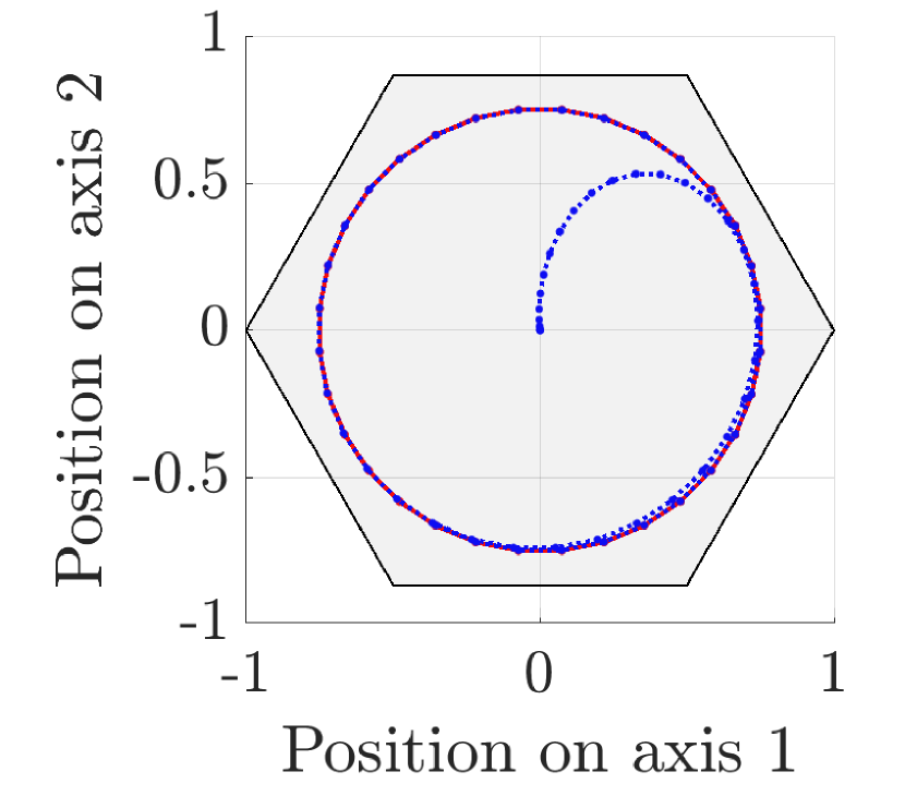
(a) HMPC (SPCIES).

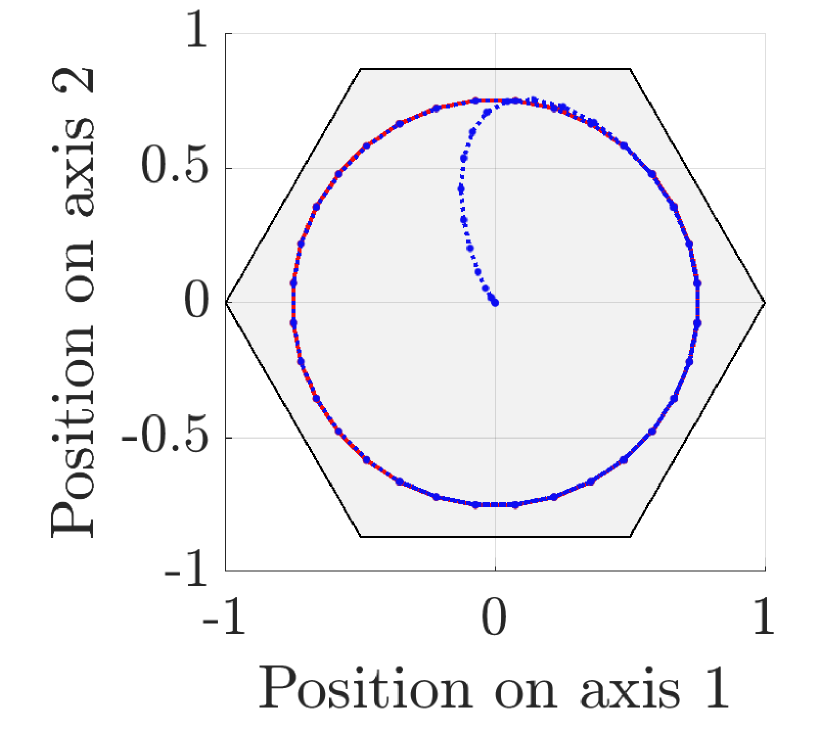
(b) MPCT (OSQP).

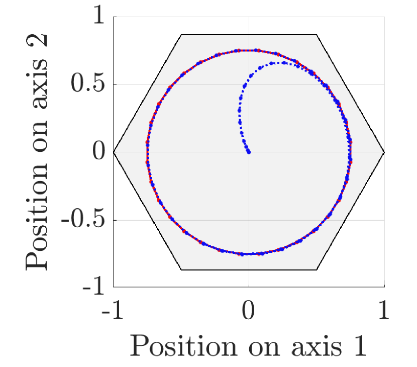
(c) stdMPC (OSQP).

Figure 2: Tracking an admissible harmonic reference.

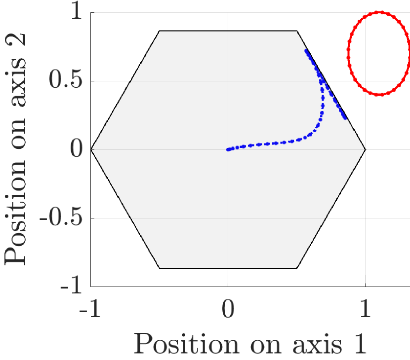
(a) HMPC (SPCIES).

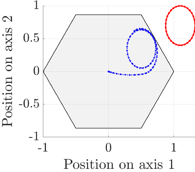
(b) HMPC with increased $T_{h}$ (SPCIES).

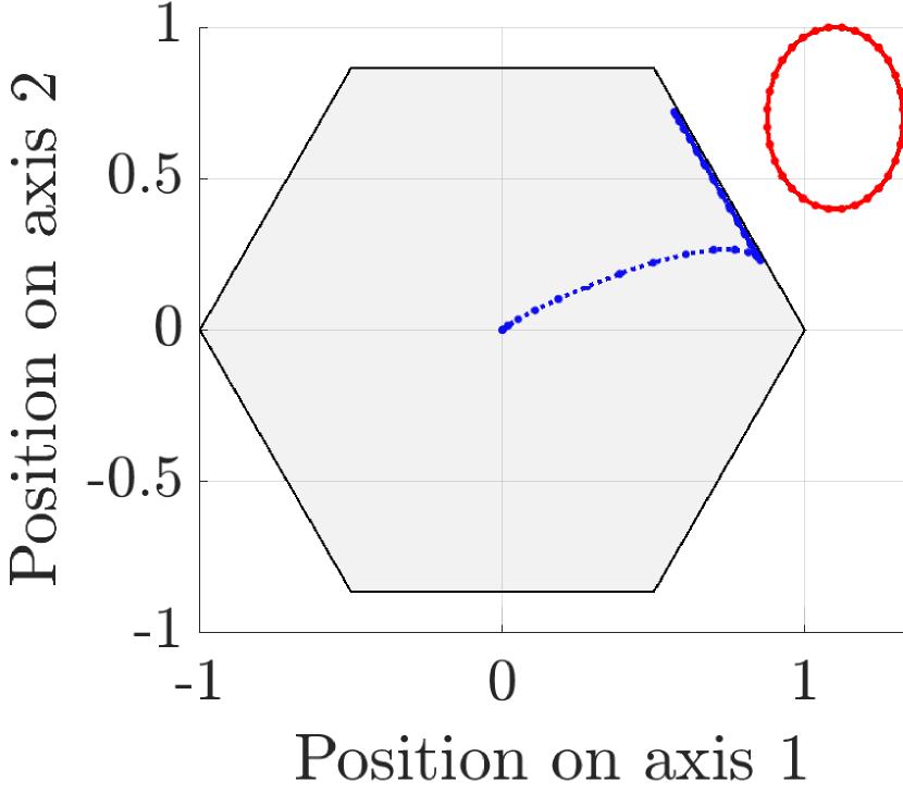
(c) MPCT (OSQP).

Figure 3: Tracking a non-admissible harmonic reference.

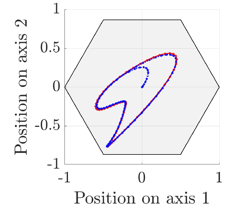
(a) Ball position on the plate.

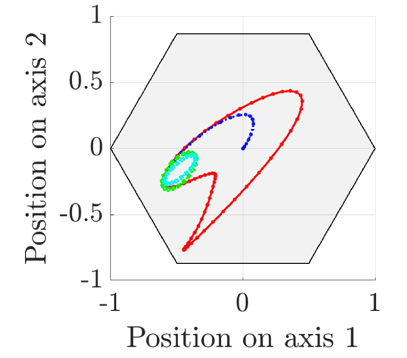
(b) $t=20$: Position on the plate.

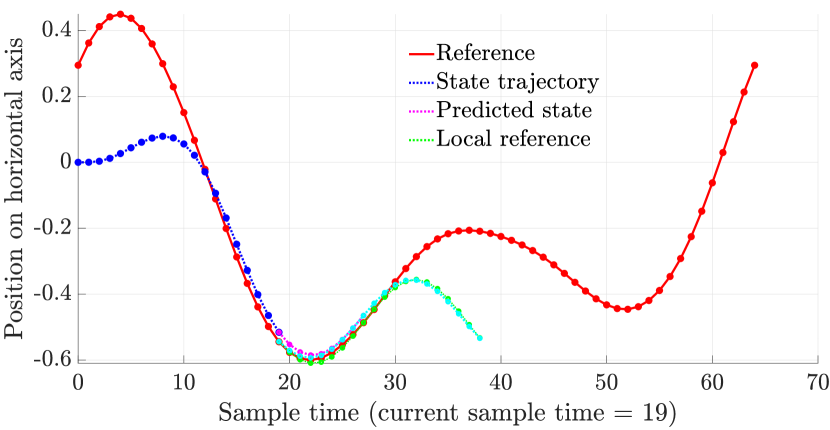
(c) $t=20$: Horizontal axis.

Figure 4: Tracking an admissible arbitrary reference using HMPC (solved using SPCIES).

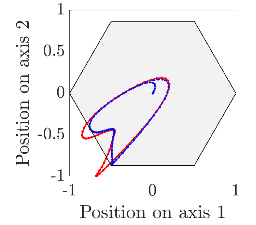
(a) Ball position on the plate.

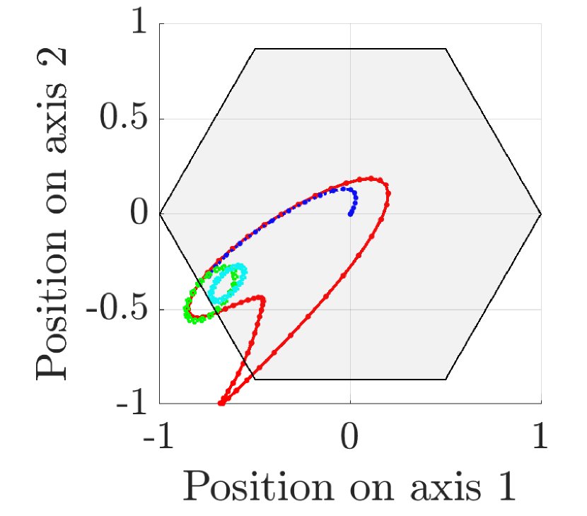
(b) $t=20$: Position on the plate.

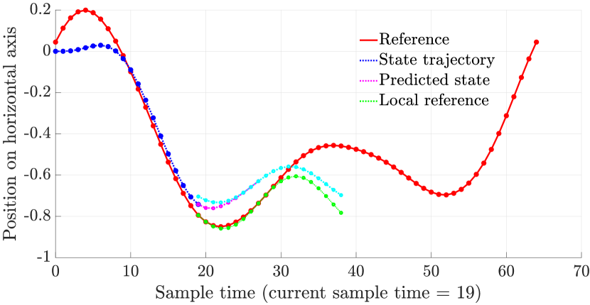
(c) $t=20$: Horizontal axis.

Figure 5: Tracking a non-admissible arbitrary reference using HMPC (solved using SPCIES).

We now show the results when controlling a reference which is not given by a harmonic signal. Instead, we take a multiple harmonic signal on the form

$$x_{r}(t) =x_{re}+\sum\limits_{i=1}^{p}x_{rs,i}\sin(iw_{r}t)+x_{rc,i}\cos(iw_{r}t),$$

$$u_{r}(t) =u_{re}+\sum\limits_{i=1}^{p}u_{rs,i}\sin(iw_{r}t)+u_{rc,i}\cos(iw_{r}t)$$

satisfying $x_{r}(t+1)=Ax_{r}(t)+Bu_{r}(t)$, $\forall t$, where we select the base frequency of the reference as $w_{r}=\pi/32$ and the number of harmonics as $p=6$. The main control objective is to control the position of the ball on the plate, which is given by two of the elements of the state vector. We maintain the same cost function matrices and prediction horizon used in the results of the previous subsection, with the exception of $T_{e}$ and $T_{h}$, which we find need to be significantly larger in this paradigm; we instead take $T_{e}=80Q$ and $T_{h}=T_{e}$. Additionally, following the guidelines of [11, §VI], we take the base frequency of the HMPC formulation as $w=0.3254$.

Figure 4 shows the closed-loop results. Figure 4(a) shows the trajectory of the ball on the plate for two periods of the reference. Figure 4(b) shows a snapshot of the trajectory at sample time $t=20$, showing the approximation of the reference described in Section IV and the artificial harmonic reference obtained from the solution of the HMPC optimization problem. Figure 4(c) shows the same snapshot but for the evolution of the position on the horizontal axis. Finally, Figure 5 shows analogous results to Figure 4 but shifting the reference so that it is (partially) non-admissible.

The results show that the HMPC formulation tracks the admissible reference reasonably well. When the reference is non-admissible, the approximation reference and the artificial reference are no longer close to each other in the areas in which the reference is non-admissible. In this case, the closed-loop trajectory resembles the desired reference in the areas in which it is non-admissible, although in the case of generic references this resemblance is no longer guaranteed, even if $T_{h}$ and $S_{h}$ are dominant. In fact, we find that the behavior of HMPC in the case of dominant $T_{h}$ and $S_{h}$ terms can be rather nonintuitive when tracking arbitrary references.

One of the potential applications of this paradigm is to track (possibly non-periodic) reference trajectories that are not completely known before hand, since the proposed approach only required knowledge of the following $N$ elements of the reference. The advantage of the HMPC controller in this case is its guaranteed recursive feasibility.

V-C Computational results

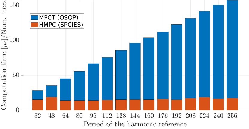
Figure 6: Results increasing the period of the reference.

Table I shows the computational results obtained with the difference MPC formulations and solvers for the tests shown in Figures 2-5. Results for Figures 2-3 are in the rows labeled with “Harmonic ref.”, and the ones for Figures 4-5 in the rows labeled with “Arb. ref.”. The table includes the computational results obtained using stdMPC for the test in Figure 3 and well as the computation times of MPCT for the tests in Figures 4-5. The computation times for HMPC related to Figure 3 are for the simulation shown in Figure 3(a).

Figure 6 shows the computation times per iteration of HMPC using SPCIES and of the periodic MPCT formulation using OSQP for increasing values of the period of the harmonic reference signal. As already discussed, the results show that the complexity of the HMPC formulation does not depend on the period of the reference. Therefore, for large reference periods, the HMPC formulation may be preferable over other alternative periodic MPC formulations whose solver iteration complexity grows with the period.

VI Conclusions

This article has presented an extension of the HMPC formulation [11] for tracking harmonic references and has discussed its application for tracking arbitrary reference trajectories. In the case of tracking harmonic references, we showed that the terminal ingredients can be chosen to penalize deviations with respect to the “shape” of the reference, which is an interesting property that may have useful practical applications. Preliminary simulations indicate that the HMPC formulation can provide good tracking of arbitrary references if its ingredients are chosen appropriately. An interesting application of this paradigm is when only the future $N$ reference values are known at any given instant. Computational results indicate that the HMPC solver proposed in [12] provides computational times that are competitive with state-of-the-art solvers. Moreover, the computation time per iteration of the solver does not depend on the period of the reference, making it an ideal candidate when working with references with large periods.

This appendix contains the proofs of Lemma 1, Theorem 1 and Theorem 2. The proofs of Theorem 1 and Theorem 2 follow the proofs of [11, Theorem 1] and [11, Theorem 3], respectively, with the modifications required for the extension to harmonic references. In the case of Theorem 1, the modifications are due to the terminal constraint (9e), which is different than the one used in [11]. As for Theorem 2, the modifications are due to the difference between the offset cost functions $V_{h}$ used in this article and in [11], as well as for the time-varying nature of the reference (7).

Proof of Lemma 1.

By definition, at $t+1$, $(\mathring{{\rm\bf{x}}}(t+1),\mathring{{\rm\bf{u}}}(t+1))$ is the optimal solution of

$$\min\limits_{{\rm\bf{x}}_{h},{\rm\bf{u}}_{h}}\; V_{h}({\rm\bf{x}}_{h},{\rm\bf{u}}_{h},\mathcal{T}_{h}^{n_{x}}{\rm\bf{x}}_{r}(t),\mathcal{T}_{h}^{n_{u}}{\rm\bf{u}}_{r}(t))$$ (11a)

$${\rm s.t.}\; ({\rm\bf{x}}_{h},{\rm\bf{u}}_{h})\in{\mathcal{D}}\cap{\mathcal{C}}_{\sigma},$$ (11b)

where we recall that $\mathcal{T}_{h}^{m}\doteq\mathtt{diag}(I_{m},\mathcal{T}_{w}^{m})$ and $\mathcal{T}_{w}^{m}$ is defined in (6). By taking the change of variables ${\rm\bf{x}}_{h}=\mathcal{T}_{h}^{n_{x}}\hat{{\rm\bf{x}}}_{h}$ and ${{\rm\bf{u}}_{h}=\mathcal{T}_{h}^{n_{u}}\hat{{\rm\bf{u}}}_{h}}$, we can recover the optimal solution of (11) from the optimal solution of

$$\min\limits_{\hat{{\rm\bf{x}}}_{h},\hat{{\rm\bf{u}}}_{h}}\;\left\{\tilde{V}_{h},\;{\rm s.t.}\,(\mathcal{T}_{h}^{n_{x}}\hat{{\rm\bf{x}}}_{h},\mathcal{T}_{h}^{n_{u}}\hat{{\rm\bf{u}}}_{h})\in{\mathcal{D}}\cap{\mathcal{C}}_{\sigma}\right\},$$ (12)

where $\tilde{V}_{h}\doteq V_{h}(\mathcal{T}_{h}^{n_{x}}\hat{{\rm\bf{x}}}_{h},\mathcal{T}_{h}^{n_{u}}\hat{{\rm\bf{u}}}_{h},\mathcal{T}_{h}^{n_{x}}{\rm\bf{x}}_{r}(t),\mathcal{T}_{h}^{n_{u}}{\rm\bf{u}}_{r}(t))$.

From Propositions 1 and 2, we have that the set ${\mathcal{D}}\cap{\mathcal{C}}_{\sigma}$ is closed under the transform $(\mathcal{T}_{h}^{n_{x}},\mathcal{T}_{h}^{n_{u}})$, i.e.,

$$(\mathcal{T}_{h}^{n_{x}}\hat{x}_{h},\mathcal{T}_{h}^{n_{u}}\hat{u}_{h})\in{\mathcal{D}}\cap{\mathcal{C}}_{\sigma}\iff(\hat{x}_{h},\hat{u}_{h})\in{\mathcal{D}}\cap{\mathcal{C}}_{\sigma}.$$

Additionally, the cost function satisfies the equality ${\tilde{V}_{h}=V_{h}(\hat{{\rm\bf{x}}}_{h},\hat{{\rm\bf{u}}}_{h},{\rm\bf{x}}_{r}(t),{\rm\bf{u}}_{r}(t))}$. Indeed, first note that the $x_{e}$ and $u_{e}$ terms of $V_{h}$ are equal due to the identity matrices in $\mathcal{T}_{h}^{n_{x}}$ and $\mathcal{T}_{h}^{n_{u}}$. Next, for the $x_{s}$, $x_{c}$, $u_{s}$, and $u_{c}$ terms, we have that for any two vectors $z,v\in\mathbb{R}^{2m}$ and $D=\mathtt{diag}(\tilde{D},\tilde{D})$, with $\tilde{D}\in\mathbb{D}_{+}^{m}$,

$$\|\mathcal{T}_{w}^{m}(z-v)\|^{2}_{D} =(z-v)^{\top}(\mathcal{T}_{w}^{m})^{\top}D\mathcal{T}_{w}^{m}(z-v)$$

$$\stackrel{{\scriptstyle\scriptstyle\mkern-1.5mu(*)\mkern-1.5mu}}{{=}}(z-v)^{\top}D(z-v)=\|z-v\|^{2}_{D},$$

where $(*)$ follows from the definition of $\mathcal{T}_{w}^{m}$ (6) and the well known identity $\sin^{2}(w)+\cos^{2}(w)=1$. The equality then follows from the fact that $T_{h}\in\mathbb{D}_{+}^{n_{x}}$ and $S_{h}\in\mathbb{D}_{+}^{n_{u}}$. Therefore, (12) is equivalent to (10), whose solution is $(\mathring{{\rm\bf{x}}}(t),\mathring{{\rm\bf{u}}}(t))$ by definition, thus $\hat{{\rm\bf{x}}}_{h}^{*}=\mathring{{\rm\bf{x}}}(t)$ and $\hat{{\rm\bf{u}}}_{h}^{*}=\mathring{{\rm\bf{u}}}(t)$. Finally, undoing the change of variables leads to $\mathring{{\rm\bf{x}}}(t+1)=\mathcal{T}_{h}^{n_{x}}\hat{{\rm\bf{x}}}_{h}^{*}=\mathcal{T}_{h}^{n_{x}}\mathring{{\rm\bf{x}}}(t)$ and $\mathring{{\rm\bf{u}}}(t+1)=\mathcal{T}_{h}^{n_{u}}\hat{{\rm\bf{u}}}_{h}^{*}=\mathcal{T}_{h}^{n_{u}}\mathring{{\rm\bf{u}}}(t)$. ∎

Proof of Theorem 1.

We show that $\tilde{{\rm\bf{x}}}$, $\tilde{{\rm\bf{u}}}$, $\tilde{{\rm\bf{x}}}_{h}$, $\tilde{{\rm\bf{u}}}_{h}$ satisfying

$$\tilde{u}^{k}=u^{k+1},\;k\in\mathbb{Z}_{0}^{N-2}$$ (13a)

$$\tilde{u}^{N-1}=u_{e}+u_{s}\sin(wN)+u_{c}\cos(wN)$$ (13b)

$$\tilde{x}^{0}=Ax(t)+Bu^{0}$$ (13c)

$$\tilde{x}^{k+1}=A\tilde{x}^{k}+B\tilde{u}^{k},\;k\in\mathbb{Z}_{0}^{N-1}$$ (13d)

$$\tilde{u}_{e}=u_{e}$$ (13e)

$$\tilde{u}_{s}=u_{s}\cos(w)-u_{c}\sin(w)$$ (13f)

$$\tilde{u}_{c}=u_{s}\sin(w)+u_{c}\cos(w)$$ (13g)

$$\begin{bmatrix}\tilde{x}_{e}&\tilde{x}_{s}&\tilde{x}_{c}\end{bmatrix}=\begin{bmatrix}A&B\end{bmatrix}\begin{bmatrix}x_{e}&x_{s}&x_{c}\\ u_{e}&u_{s}&u_{c}\end{bmatrix}$$ (13h)

is a feasible solution of problem (9) for the successor state $Ax(t)+Bu^{0}$ by showing that (13) satisfies (9b)-(9g). That is, we prove in what follows that

$$\tilde{x}^{0}=Ax(t)+Bu^{0}$$ (14a)

$$\tilde{x}^{k+1}=A\tilde{x}^{k}+B\tilde{u}^{k},\;k\in\mathbb{Z}_{0}^{N-1}$$ (14b)

$$\underline{y}\leq E\tilde{x}^{k}+F\tilde{u}^{k}\leq\overline{y},\;k\in\mathbb{Z}_{0}^{N-1}$$ (14c)

$$\tilde{x}^{N}=\tilde{x}_{e}+\tilde{x}_{s}\sin(wN)+\tilde{x}_{c}\cos(wN)$$ (14d)

$$\tilde{x}_{e}=A\tilde{x}_{e}+B\tilde{u}_{e}$$ (14e)

$$\tilde{x}_{s}\cos(w)-\tilde{x}_{c}\sin(w)=A\tilde{x}_{s}+B\tilde{u}_{s}$$ (14f)

$$\tilde{x}_{s}\sin(w)+\tilde{x}_{c}\cos(w)=A\tilde{x}_{c}+B\tilde{u}_{c}$$ (14g)

$$\sqrt{\tilde{y}_{s(i)}^{2}+\tilde{y}_{c(i)}^{2}}\leq\overline{y}_{(i)}-\sigma-\tilde{y}_{e(i)},\;i\in\mathbb{Z}_{1}^{n_{y}},$$ (14h)

$$\sqrt{\tilde{y}_{s(i)}^{2}+\tilde{y}_{c(i)}^{2}}\leq\tilde{y}_{e(i)}-\underline{y}_{(i)}-\sigma,\;i\in\mathbb{Z}_{1}^{n_{y}},$$ (14i)

where $\tilde{y}_{e}$, $\tilde{y}_{s}$ and $\tilde{y}_{c}$ are given by

$$\tilde{y}_{e}\doteq E\tilde{x}_{e}+F\tilde{u}_{e},\;\tilde{y}_{s}\doteq E\tilde{x}_{s}+F\tilde{u}_{s},\;\tilde{y}_{c}\doteq E\tilde{x}_{c}+F\tilde{u}_{c}.$$

Equalities (14a) and (14b) are trivially satisfied by construction, see (13c) and (13d). From (13a) and $\tilde{x}^{0}=Ax(t)+Bu^{0}=x^{1}$, we have

$$\tilde{x}^{k}=x^{k+1},\;\tilde{u}^{k}=u^{k+1},\;k\in\mathbb{Z}_{0}^{N-2}.$$ (15)

Therefore, from (9d) we obtain

$$\underline{y}\leq E\tilde{x}^{k}+F\tilde{u}^{k}\leq\overline{y},\;k\in\mathbb{Z}_{0}^{N-2}.$$ (16)

Let $\tilde{y}^{k}\doteq E\tilde{x}^{k}+F\tilde{u}^{k}$. Using (9e), we have that

$$\tilde{x}^{N-1} =A\tilde{x}^{N-2}+B\tilde{u}^{N-2}=Ax^{N-1}+Bu^{N-1}$$ (17)

$$=x^{N}=x_{e}+x_{s}\sin(wN)+x_{c}\cos(wN).$$

Thus, using (13b), we obtain

$$\tilde{y}^{N-1}=y_{e}+y_{s}\sin(wN)+y_{c}\cos(wN),$$

which, making use of Proposition 2 along with (9g) and the fact that $\sigma>0$, leads to $\underline{y}\leq\tilde{y}^{N-1}\leq\overline{y}$, i.e.,

$$\underline{y}\leq E\tilde{x}^{N-1}+F\tilde{u}^{N-1}\leq\overline{y}.$$

This, along with (16), proves (14c). The value of $\tilde{x}^{N}$ can be computed from $\tilde{x}^{N-1}=x^{N}$ and $\tilde{u}^{N-1}$ as follows:

$$\tilde{x}^{N} =A\tilde{x}^{N-1}+B\tilde{u}^{N-1}=Ax^{N}+B\tilde{u}^{N-1}$$

$$=A(x_{e}+x_{s}\sin(wN)+x_{c}\cos(wN))$$

$$\quad+B(u_{e}+u_{s}\sin(wN)+u_{c}\cos(wN))$$

$$=\tilde{x}_{e}+\tilde{x}_{s}\sin(wN)+\tilde{x}_{c}\cos(wN),$$

which proves (14d). From $\tilde{x}_{e}=Ax_{e}+Bu_{e}=x_{e}$ and $\tilde{u}_{e}=u_{e}$ we have $\tilde{x}_{e}=A\tilde{x}_{e}+B\tilde{u}_{e}$, which proves (14e). We now prove (14f) and (14g) as follows:

$$A\tilde{x}_{s}+B\tilde{u}_{s} =A(Ax_{s}+Bu_{s})+B(u_{s}\cos(w)-u_{c}\sin(w))$$

$$=(Ax_{s}+Bu_{s})\cos(w)-(Ax_{c}+Bu_{c})\sin(w)$$

$$=\tilde{x}_{s}\cos(w)-\tilde{x}_{c}\sin(w),$$

$$A\tilde{x}_{c}+B\tilde{u}_{c} =A(Ax_{c}+Bu_{c})+B(u_{s}\sin(w)+u_{c}\cos(w))$$

$$=(Ax_{s}+Bu_{s})\sin(w)+(Ax_{c}+Bu_{c})\cos(w)$$

$$=\tilde{x}_{s}\sin(w)+\tilde{x}_{c}\cos(w).$$

Next, we express $\tilde{y}_{e}$, $\tilde{y}_{s}$ and $\tilde{y}_{c}$ in terms of $y_{e}$, $y_{s}$ and $y_{c}$:

$$\tilde{y}_{e} =E\tilde{x}_{e}+F\tilde{u}_{e}=Ex_{e}+Fu_{e}=y_{e},$$

$$\tilde{y}_{s} =E\tilde{x}_{s}+F\tilde{u}_{s}=E(Ax_{s}+Bu_{s})+F\tilde{u}_{s}$$

$$=E(x_{s}\cos(w)-x_{c}\sin(w))+F(u_{s}\cos(w)-u_{c}\sin(w))$$

$$=(Ex_{s}+Fu_{s})\cos(w)-(Ex_{c}+Fu_{c})\sin(w)$$

$$=y_{s}\cos(w)-y_{c}\sin(w),$$

$$\tilde{y}_{c} =E\tilde{x}_{c}+F\tilde{u}_{c}=E(Ax_{c}+Bu_{c})+F\tilde{u}_{c}$$

$$=E(x_{s}\sin(w)+x_{c}\cos(w))+F(u_{s}\sin(w)+u_{c}\cos(w))$$

$$=(Ex_{s}+Fu_{s})\sin(w)+(Ex_{c}+Fu_{c})\cos(w)$$

$$=y_{s}\sin(w)+y_{c}\cos(w).$$

Therefore, for every $i\in\mathbb{Z}_{1}^{n_{y}}$ we have $\tilde{y}_{e(i)}=y_{e(i)}$,

$$\tilde{y}_{s(i)}=y_{s(i)}\cos(w)-y_{c(i)}\sin(w),$$

$$\tilde{y}_{c(i)}=y_{s(i)}\sin(w)+y_{c(i)}\cos(w),$$

which in view of [11, Property 1] leads to

$$\sqrt{\tilde{y}_{s(i)}^{2}+\tilde{y}_{c(i)}^{2}}=\sqrt{y_{s(i)}^{2}+y_{c(i)}^{2}},\;i\in\mathbb{Z}_{1}^{n_{y}},$$

from where we conclude that (14h) and (14i) are directly inferred from (9g).∎

The proof of Theorem 2 relies on the following lemma, which revisits [11, Lemma 2] to problem (9), i.e., to account for the time-varying nature of the harmonic reference (7).

Lemma 2.

Consider a system (2) subject to (3) and assume that $N$ is greater or equal to its controllability index. Let $(x_{r}(t),u_{r}(t))$ be a given harmonic reference, $x(t)$ be a state belonging to the feasibility region of the HMPC controller (9), and ${\rm\bf{x}}^{*}$, ${\rm\bf{u}}^{*}$, ${\rm\bf{x}}_{h}^{*}$ and ${\rm\bf{u}}_{h}^{*}$ be its corresponding optimal solution. Then, $x(t)=x_{e}^{*}+x_{c}^{*}$ if and only if $x(t)=\mathring{x}(t)$.

Proof.

For space considerations, we drop the dependency w.r.t. $({\rm\bf{x}}_{r}(t),{\rm\bf{u}}_{r}(t))$ from the notation. First, we show the implication $x(t)=x_{e}^{*}+x_{c}^{*}\implies x(t)=\mathring{x}(t)$.

Assume that $x(t)=x_{e}^{*}+x_{c}^{*}$ and let $V_{h}^{*}\doteq V_{h}({\rm\bf{x}}_{h}^{*},{\rm\bf{u}}_{h}^{*})$, $V_{h}^{\circ}\doteq V_{h}(\mathring{{\rm\bf{x}}}(t),\mathring{{\rm\bf{u}}}(t))$, and $\mathbb{H}^{*}(x(t))$ be the optimal value of (9) for $x(t)$. We now shown that $\mathbb{H}^{*}(x(t))=V_{h}^{*}$, i.e., that the optimal solution of (9) is given by

$$x_{*}^{k}=x_{h*}^{k},\quad u_{*}^{k}=u_{h*}^{k},\quad\forall k\in\mathbb{Z}_{0}^{N-1},$$ (18)

where $\{x_{*}^{k}\}$, $\{u_{*}^{k}\}$, $\{x_{h*}^{k}\}$ and $\{u_{h*}^{k}\}$ are the optimal sequences parameterized by the optimal solution ${\rm\bf{x}}^{*}$, ${\rm\bf{u}}^{*}$, ${\rm\bf{x}}_{h}^{*}$ and ${\rm\bf{u}}_{h}^{*}$ of problem (9). Indeed, the stage cost of (18) is $\ell_{h}(x_{*}^{k},u_{*}^{k},x_{h*}^{k},u_{h*}^{k})=0$, $k\in\mathbb{Z}_{0}^{N-1}$, which is its smallest possible value, and it is easy to show that (18) is a feasible solution of (9). Taking this into account, we prove that $V_{h}^{*}=V_{h}^{\circ}$ by contradiction. Assume that $V_{h}^{*}>V_{h}^{\circ}$. Since $(\mathring{{\rm\bf{x}}}(t),\mathring{{\rm\bf{u}}}(t))$ is the unique minimizer of $V_{h}(\cdot)$ for all $({\rm\bf{x}}_{h},{\rm\bf{u}}_{h})\in{\mathcal{D}}\cap{\mathcal{C}}_{\sigma}$, this implies that $({\rm\bf{x}}_{h}^{*},{\rm\bf{u}}_{h}^{*})\neq(\mathring{{\rm\bf{x}}}(t),\mathring{{\rm\bf{u}}}(t))$. Let $\hat{{\rm\bf{x}}}_{h}$ be defined as

$$\hat{{\rm\bf{x}}}_{h} =(\hat{x}_{e},\hat{x}_{s},\hat{x}_{c})=\lambda{\rm\bf{x}}_{h}^{*}+(1-\lambda)\mathring{{\rm\bf{x}}}(t)$$

$$=\lambda(x_{e}^{*},x_{s}^{*},x_{c}^{*})+(1-\lambda)(\mathring{x}_{e}(t),\mathring{x}_{s}(t),\mathring{x}_{c}(t)),\;\lambda\in[0,1],$$

and $\hat{{\rm\bf{u}}}_{h}$ similarly. Let

$${\mathcal{Y}}\doteq\left\{(x,u)\in\mathbb{R}^{n_{x}}\times\mathbb{R}^{n_{u}}:\underline{y}\leq Ex+Fu\leq\overline{y}\right\}.$$ (19)

From Proposition 2 and the fact that $({\rm\bf{x}}_{h}^{*},{\rm\bf{u}}_{h}^{*})$ satisfies (9g), we have that $(x_{h*}^{k},u_{h*}^{k})\in{\rm ri}({\mathcal{Y}})$ for all $k\in\mathbb{Z}$. This, along with the assumption that $N$ is greater or equal to the controllability index of the system, implies the existence of a $\hat{\lambda}\in[0,1)$ such that for any $\lambda\in[\hat{\lambda},1]$ there is a dead-beat control law ${\rm\bf{u}}_{\text{db}}$ for which the predicted trajectory ${\rm\bf{x}}_{\text{db}}$ satisfying $x_{\text{db}}^{0}=x_{h*}^{0}=x_{e}^{*}+x_{c}^{*}$ and $x_{\text{db}}^{N}=\hat{x}_{h}^{N}$ is a feasible solution $({\rm\bf{x}}_{\text{db}},{\rm\bf{u}}_{\text{db}},\hat{{\rm\bf{x}}}_{h},\hat{{\rm\bf{u}}}_{h})$ of problem $\mathbb{H}(x_{e}^{*}+x_{c}^{*})$. Taking into account the optimality of (18), and noting that there exists a matrix $P\in\mathbb{S}_{+}^{n}$ such that

$$\sum\limits_{k=0}^{N-1}\|x_{\text{db}}^{k}-\hat{x}_{h}^{k}\|^{2}_{Q}+\|u_{\text{db}}^{k}-\hat{u}_{h}^{k}\|^{2}_{R}\leq\|x_{\text{db}}^{0}-\hat{x}_{h}^{0}\|^{2}_{P},$$

we have that

$$V_{h}^{*} \leq\|x_{h*}^{0}-\hat{x}_{h}^{0}\|^{2}_{P}+V_{h}(\hat{{\rm\bf{x}}}_{h},\hat{{\rm\bf{u}}}_{h})$$

$$\stackrel{{\scriptstyle\scriptstyle\mkern-1.5mu(*)\mkern-1.5mu}}{{=}}(1-\lambda)^{2}\|x_{h*}^{0}-\mathring{x}(t)\|^{2}_{P}+V_{h}(\hat{{\rm\bf{x}}}_{h},\hat{{\rm\bf{u}}}_{h}),$$ (20)

where step $(*)$ is using

$$x_{h*}^{0}-\hat{x}_{h}^{0}=x_{h*}^{0}{-}(\lambda x_{h*}^{0}-(1{-}\lambda)\mathring{x}(t))=(1{-}\lambda)(x_{h*}^{0}-\mathring{x}(t)).$$

From the convexity of $V_{h}(\cdot)$ we have that

$$V_{h}(\hat{{\rm\bf{x}}}_{h},\hat{{\rm\bf{u}}}_{h})\leq\lambda V_{h}^{*}+(1-\lambda)V_{h}^{\circ},\;\lambda\in[0,1],$$

which combined with (VI) leads to,

$$V_{h}^{*}\leq\theta(\lambda),\,\lambda\in[\hat{\lambda},1],$$ (21)

where

$$\theta(\lambda)\doteq(1-\lambda)^{2}\|x_{h*}^{0}-\mathring{x}(t)\|^{2}_{P}+\lambda(V_{h}^{*}-V_{h}^{\circ})+V_{h}^{\circ}.$$

The derivative of $\theta(\lambda)$ (w.r.t. $\lambda$) is

$$\theta^{\prime}(\lambda)=-2(1-\lambda)\|x_{h*}^{0}-\mathring{x}(t)||^{2}_{P}+(V_{h}^{*}-V_{h}^{\circ}).$$

Taking into account the initial assumption $V_{h}^{*}-V_{h}^{\circ}>0$, we have that $\theta^{\prime}(1)>0$. Therefore, there exists a $\lambda\in[\hat{\lambda},1)$ such that $\theta(\lambda)<\theta(1)=V_{h}^{*}$, which together with (21) leads to the contradiction $V_{h}^{*}<V_{h}^{*}$. Therefore, we have that $V_{h}^{*}\leq V_{h}^{\circ}$. Moreover, since $(\mathring{{\rm\bf{x}}},\mathring{{\rm\bf{u}}})$ is the unique minimizer of $V_{h}({\rm\bf{x}}_{h},{\rm\bf{u}}_{h})$ for all $({\rm\bf{x}}_{h},{\rm\bf{u}}_{h})$ satisfying $({\rm\bf{x}}_{h},{\rm\bf{u}}_{h})\in{\mathcal{D}}\cap{\mathcal{C}}_{\sigma}$, we conclude that $x_{h*}^{0}=x_{e}^{*}+x_{c}^{*}=\mathring{x}(t)$.

The reverse implication is straightforward. Assume now that ${x(t)=\mathring{x}(t)}$. Then,

$${\rm\bf{x}}_{h}^{*}=\mathring{{\rm\bf{x}}}(t),\,{\rm\bf{u}}_{h}^{*}=\mathring{{\rm\bf{u}}}(t),\,x_{*}^{k}=\mathring{x}^{k},\,u_{*}^{k}=\mathring{u}^{k},\,k\in\mathbb{Z}_{0}^{N-1},$$ (22)

is a feasible solution of $\mathbb{H}(x(t))$, since $(\mathring{{\rm\bf{x}}}(t),\mathring{{\rm\bf{u}}}(t))\in{{\mathcal{D}}\cap{\mathcal{C}}_{\sigma}}$ and $(\mathring{x}^{k},\mathring{u}^{k})$ satisfies the system dynamics and constraints (c.f., [11]). Moreover, (22) is the optimal solution of $\mathbb{H}(x(t))$. Indeed, $\ell_{h}(x_{*}^{k},u_{*}^{k},x_{h*}^{k},u_{h*}^{k})=0$, $k\in\mathbb{Z}_{0}^{N-1}$, and $V_{h}^{*}=V_{h}^{\circ}$, which is, once again, its minimum value for all $({\rm\bf{x}}_{h},{\rm\bf{u}}_{h})\in{\mathcal{D}}\cap{\mathcal{C}}_{\sigma}$. Therefore, due to the strict convexity of $V_{h}(\cdot)$, we conclude that ${\rm\bf{x}}_{h}^{*}=\mathring{{\rm\bf{x}}}(t)$, implying $x_{h*}^{0}=x_{e}^{*}+x_{c}^{*}=\mathring{x}(t)$. ∎

The proof of Theorem 2 is based on finding a function that satisfies the Lyapunov conditions for asymptotic stability given in the following theorem [2, Appendix B.3].

Theorem 3 (Lyapunov asymptotic stability).

Consider an autonomous system $z(t+1)=f(z(t))$ with states $z(t)\in\mathbb{R}^{n}$ and where the function $f:\mathbb{R}^{n}\rightarrow\mathbb{R}^{n}$ is continuous and satisfies $f(0)=0$. Let $\Gamma$ be a positive invariant set and $\Omega\subseteq\Gamma$ be a compact set, both including the origin as an interior point. If there exists a function $W:\mathbb{R}^{n}\rightarrow\mathbb{R}_{+}$ and suitable ${\mathcal{K}}_{\infty}$-class functions $\alpha_{1}(\cdot)$ and $\alpha_{2}(\cdot)$ such that,

1. $W(z(t))\geq\alpha_{1}(\|z(t)\|),\;\forall z_{k}\in\Gamma,$

2. $W(z(t))\leq\alpha_{2}(\|z(t)\|),\;\forall z_{k}\in\Omega,$

3. $W(z(t+1))<W(z(t)),\forall z(t)\in\Gamma\setminus\{0\},$
   and $W(z(t+1))=W(z(t))$ if $z(t)=0$,

then $W$ is a Lyapunov function for $z(t+1)=f(z(t))$ in $\Gamma$ and the origin is asymptotically stable for all initial states in $\Gamma$.

Proof of Theorem 2.

Let us consider a state $x(t)$ belonging to the domain of attraction of the HMPC controller and a harmonic reference parameterized by $({\rm\bf{x}}_{r}(t),{\rm\bf{u}}_{r}(t))$. Due to space considerations, in this proof we will drop the dependency w.r.t. $({\rm\bf{x}}_{r}(t),{\rm\bf{u}}_{r}(t))$ from the notation of the functions. Let ${\rm\bf{x}}^{*}$, ${\rm\bf{u}}^{*}$, ${\rm\bf{x}}_{h}^{*}$, ${\rm\bf{u}}_{h}^{*}$ be the optimal solution of $\mathbb{H}(x(t))$, $\mathbb{H}^{*}(x(t))$ be its optimal value, $V_{h}^{*}\doteq V_{h}({\rm\bf{x}}_{h}^{*},{\rm\bf{u}}_{h}^{*})$ and $V_{h}^{\circ}\doteq V_{h}(\mathring{{\rm\bf{x}}}(t),\mathring{{\rm\bf{u}}}(t))$. Furthermore, let $\{x_{*}^{k}\}$, $\{u_{*}^{k}\}$, $\{x_{h*}^{k}\}$ and $\{u_{h*}^{k}\}$ be the optimal sequences parameterized by the optimal solution ${\rm\bf{x}}^{*}$, ${\rm\bf{u}}^{*}$, ${\rm\bf{x}}_{h}^{*}$ and ${\rm\bf{u}}_{h}^{*}$. We will now show that the function

$$W(z(t))=\mathbb{H}^{*}(x(t))-V_{h}^{\circ}$$

is a Lyapunov function for $z(t)=x(t)-\mathring{x}(t)$ by finding suitable $\alpha_{1}(\|x(t)-\mathring{x}(t)\|)$ and $\alpha_{2}(\|x(t)-\mathring{x}(t)\|)$ ${\mathcal{K}}_{\infty}$-class functions such that the conditions of Theorem 3 are satisfied.

We now prove that there exists $\mu>0$ such that Theorem 3.(i) is satisfied for any state $x(t)$ belonging to the domain of attraction of the HMPC controller. Indeed,

$$W(z(t)) =\sum\limits_{k=0}^{N-1}\|x_{*}^{k}-x_{h*}^{k}\|_{Q}^{2}+\|u_{*}^{k}-u_{h*}^{k}\|_{R}^{2}+V_{h}^{*}-V_{h}^{\circ}$$

$$\stackrel{{\scriptstyle\scriptstyle\mkern-1.5mu(*)\mkern-1.5mu}}{{\geq}}\|{x_{*}^{0}}{-}{x_{h*}^{0}}\|_{Q}^{2}+\frac{\mu}{4}\|x_{h*}^{0}-\mathring{x}(t)\|^{2}$$

$$\geq\min\{\underline{\lambda}(Q),\frac{\mu}{4}\}\left(\|x(t)-x_{h*}^{0}\|^{2}+\|x_{h*}^{0}-\mathring{x}(t)\|^{2}\right)$$

$$\stackrel{{\scriptstyle\scriptstyle\mkern-1.5mu(\dagger)\mkern-1.5mu}}{{\geq}}\frac{1}{2}\min\{\underline{\lambda}(Q),\frac{\mu}{4}\}\|x(t)-\mathring{x}(t)\|^{2},$$ (23)

where $\underline{\lambda}(Q)$ is the minimum eigenvalue of $Q$, $(\dagger)$ is due to the parallelogram law, which states that for any two vectors $v_{1},v_{2}\in\mathbb{R}^{n_{v}}$,

$$\|v_{1}\|^{2}+\|v_{2}\|^{2}=\frac{1}{2}\|v_{1}+v_{2}\|^{2}+\frac{1}{2}\|v_{1}-v_{2}\|^{2},$$ (24)

and $(*)$ follows from the fact that

$$V_{h}^{*}-V_{h}^{\circ}\geq\frac{\mu}{4}\|x_{h*}^{0}-\mathring{x}(t)\|^{2}$$ (25)

for some $\mu>0$. To show this, note that $V_{h}(\cdot)$ is a strongly convex function. Therefore, it satisfies for some $\mu>0$ [20, Theorem 5.24], [21, §9.1.2],

$$V_{h}(z)-V_{h}(y)\geq\langle\nabla V_{h}(y),z-y\rangle+\frac{\mu}{2}\|z-y\|^{2},$$

for all $z,y$, which, when particularized to $z=({\rm\bf{x}}_{h}^{*},{\rm\bf{u}}_{h}^{*})$ and $y=(\mathring{{\rm\bf{x}}}(t),\mathring{{\rm\bf{u}}}(t))$, leads to

$$V_{h}^{*}-V_{h}^{\circ} \geq\langle\nabla V_{h}^{\circ},({\rm\bf{x}}_{h}^{*},{\rm\bf{u}}_{h}^{*})-(\mathring{{\rm\bf{x}}}(t),\mathring{{\rm\bf{u}}}(t))\rangle$$

$$\quad+\frac{\mu}{2}\|({\rm\bf{x}}_{h}^{*},{\rm\bf{u}}_{h}^{*})-(\mathring{{\rm\bf{x}}}(t),\mathring{{\rm\bf{u}}}(t))\|^{2}.$$

From the optimality of $(\mathring{{\rm\bf{x}}}(t),\mathring{{\rm\bf{u}}}(t))$ we have that [22, Proposition 5.4.7], [21, §4.2.3],

$$\langle\nabla V_{h}^{\circ},({\rm\bf{x}}_{h},{\rm\bf{u}}_{h})-(\mathring{{\rm\bf{x}}}(t),\mathring{{\rm\bf{u}}}(t))\rangle\geq 0$$

for all $({\rm\bf{x}}_{h},{\rm\bf{u}}_{h})\in{\mathcal{D}}\cap{\mathcal{C}}_{\sigma}$. Since $({\rm\bf{x}}_{h}^{*},{\rm\bf{u}}_{h}^{*})\in{\mathcal{D}}\cap{\mathcal{C}}_{\sigma}$, we have

$$V_{h}^{*}-V_{h}^{\circ}\geq\frac{\mu}{2}\|({\rm\bf{x}}_{h}^{*},{\rm\bf{u}}_{h}^{*})-(\mathring{{\rm\bf{x}}}(t),\mathring{{\rm\bf{u}}}(t))\|^{2}$$

$$=\frac{\mu}{2}\left(\|{\rm\bf{x}}_{h}^{*}-\mathring{{\rm\bf{x}}}(t)\|^{2}+\|{\rm\bf{u}}_{h}^{*}-\mathring{{\rm\bf{u}}}(t)\|^{2}\right)$$

$$\geq\frac{\mu}{2}(\|x_{e}^{*}-\mathring{x}_{e}(t)\|^{2}+\|x_{s}^{*}-\mathring{x}_{s}(t)\|^{2}+\|x_{c}^{*}-\mathring{x}_{c}(t)\|^{2})$$

$$\geq\frac{\mu}{2}(\|x_{e}^{*}-\mathring{x}_{e}(t)\|^{2}+\|x_{c}^{*}-\mathring{x}_{c}(t)\|^{2}).$$

Finally, using (24), inequality (25) follows from

$$\frac{\mu}{2}(\|x_{e}^{*}-\mathring{x}_{e}(t)\|^{2}+\|x_{c}^{*}-\mathring{x}_{c}(t)\|^{2})$$

$$\geq\frac{\mu}{4}\|x_{e}^{*}-\mathring{x}_{e}(t)+x_{c}^{*}-\mathring{x}_{c}(t)\|^{2}=\frac{\mu}{4}\|x_{h*}^{0}-\mathring{x}(t)\|^{2}.$$

Since $(\mathring{x}(t),\mathring{u}(t))\in{\rm ri}({\mathcal{Y}})$, where ${\mathcal{Y}}$ is defined in (19), the system is controllable and $N$ is greater than its controllability index, there exists a sufficiently small compact set $\Omega$ containing the origin in its interior such that, for all states $x(t)$ that satisfy $x(t)-\mathring{x}(t)\in\Omega$, the dead-beat control law

$$u_{\text{db}}^{k}=K_{\text{db}}(x_{\text{db}}^{k}-\mathring{x}(t))+\mathring{u}(t)$$

provides an admissible predicted trajectory ${\rm\bf{x}}_{\text{db}}$ of system (2) subject to (3), where $x_{\text{db}}^{k+1}=Ax_{\text{db}}^{k}+Bu_{\text{db}}^{k},\;k\in\mathbb{Z}_{0}^{N-1}$, ${x_{\text{db}}^{0}=x(t)}$ and ${x_{\text{db}}^{N}=\mathring{x}^{N}}$. Then, taking into account the optimality of ${\rm\bf{x}}^{*}$, ${\rm\bf{u}}^{*}$, ${\rm\bf{x}}_{h}^{*}$, ${\rm\bf{u}}_{h}^{*}$, we have that,

$$W(z(t)) =\sum\limits_{k=0}^{N-1}\ell_{h}(x^{k}_{*},u^{k}_{*},x_{h*}^{k},u_{h*}^{k})+V_{h}({\rm\bf{x}}_{h}^{*},{\rm\bf{u}}_{h}^{*})-V_{h}^{\circ}$$

$$\leq\sum\limits_{k=0}^{N-1}\ell_{h}(x^{k}_{\text{db}},u^{k}_{\text{db}},\mathring{x}^{k},\mathring{u}^{k})+V_{h}(\mathring{{\rm\bf{x}}}(t),\mathring{{\rm\bf{u}}}(t))-V_{h}^{\circ}$$

$$=\sum\limits_{k=0}^{N-1}\|x_{\text{db}}^{k}-\mathring{x}^{k}\|^{2}_{Q}+\|u_{\text{db}}^{k}-\mathring{u}^{k}\|^{2}_{R}.$$

Therefore, there exists a matrix $P\in\mathbb{S}_{+}^{n}$ such that

$$W(z(t))\leq\overline{\lambda}(P)\|x^{0}_{\text{db}}-\mathring{x}^{0}\|^{2}=\overline{\lambda}(P)\|x(t)-\mathring{x}(t)\|^{2}$$

for any $x(t)-\mathring{x}(t)\in\Omega$, where $\overline{\lambda}(P)$ is the maximum eigenvalue of $P$. This shows the satisfaction of Theorem 3.(ii).

Let $x(t+1)\doteq Ax(t)+B\tilde{u}_{*}^{0}$ be the successor state and consider the shifted sequence $\tilde{{\rm\bf{x}}}$, $\tilde{{\rm\bf{u}}}$, $\tilde{{\rm\bf{x}}}_{h}$, $\tilde{{\rm\bf{u}}}_{h}$ be defined as in (13) but taking ${\rm\bf{x}}^{*}$, ${\rm\bf{u}}^{*}$, ${\rm\bf{x}}_{h}^{*}$, ${\rm\bf{u}}_{h}^{*}$ in the right-hand-side of the equations. It is clear from the proof of Theorem 1 that this shifted sequence is a feasible solution of $\mathbb{H}(x(t+1))$.

Let $\Delta W(z(t))\doteq W(z(t+1))-W(z(t))$ and note that, as shown by (13b), (13h), (15), (17) and [11, Property 1], we have that ${\tilde{x}^{k}=x^{k+1}_{*}}$ for $k\in\mathbb{Z}_{0}^{N-1}$, $\tilde{u}^{k}=u^{k+1}_{*}$ for $k\in\mathbb{Z}_{0}^{N-2}$, and that $\tilde{x}_{h}^{k}=x_{h*}^{k+1}$ and $\tilde{u}_{h}^{k}=u_{h*}^{k+1}$ for $k\in\mathbb{Z}$. Then,

$$\Delta W(z(t)) =\mathbb{H}^{*}(x(t+1))-V_{h}^{\circ}-\mathbb{H}^{*}(x(t))+V_{h}^{\circ}$$

$$\leq\mathbb{H}(x(t+1))-\mathbb{H}^{*}(x(t))$$

$$=\sum\limits_{k=0}^{N-1}\|\tilde{x}^{k}-\tilde{x}_{h}^{k}\|_{Q}^{2}+\|\tilde{u}^{k}-\tilde{u}_{h}^{k}\|_{R}^{2}$$

$$-\sum\limits_{k=0}^{N-1}\|x_{*}^{k}-x_{h*}^{k}\|_{Q}^{2}+\|u_{*}^{k}-u_{h*}^{k}\|_{R}^{2}$$

$$+V_{h}(\tilde{{\rm\bf{x}}}_{h},\tilde{{\rm\bf{u}}}_{h})-V_{h}({\rm\bf{x}}_{h}^{*},{\rm\bf{u}}_{h}^{*})$$

$$\stackrel{{\scriptstyle\scriptstyle\mkern-1.5mu(*)\mkern-1.5mu}}{{=}}\sum\limits_{k=1}^{N-1}\|x_{*}^{k}-x_{h*}^{k}\|_{Q}^{2}+\|u_{*}^{k}-u_{h*}^{k}\|_{R}^{2}$$

$$-\sum\limits_{k=0}^{N-1}\|x_{*}^{k}-x_{h*}^{k}\|_{Q}^{2}+\|u_{*}^{k}-u_{h*}^{k}\|_{R}^{2}$$

$$+\|x_{*}^{N}-x_{h*}^{N}\|_{Q}^{2}+\|\tilde{u}^{N-1}-u_{h*}^{N}\|_{R}^{2}$$

$$=-\|x_{*}^{0}-x_{h*}^{0}\|_{Q}^{2}-\|u_{0}^{*}-u_{h*}^{0}\|_{R}^{2}$$

$$\leq-\underline{\lambda}(Q)\|x(t)-x_{h*}^{0}\|^{2},$$

where in step $(*)$ we are making use of the fact that $V_{h}(\tilde{{\rm\bf{x}}}_{h},\tilde{{\rm\bf{u}}}_{h})=V_{h}({\rm\bf{x}}_{h}^{*},{\rm\bf{u}}_{h}^{*})$, which is proven using the same arguments used in the proof of Lemma 1 taking into account that the reference is assumed to be a harmonic signal with the same base frequency as the artificial harmonic reference, and $\|x_{*}^{N}-x_{h*}^{N}\|_{Q}^{2}+\|\tilde{u}^{N-1}-u_{h*}^{N}\|_{R}^{2}=0$ due to (9e) and (13b). The satisfaction of Theorem 3.(iii) now follows from noting that $W(z(t+1))-W(z(t))\leq-\underline{\lambda}(Q)\|x(t)-(x_{e}^{*}+x_{c}^{*})\|^{2}$ along with Lemma 2 leads to

$$W(z(t+1))<W(z(t)),\;\forall x(t)\neq\mathring{x}(t),$$

$$W(z(t+1))=W(z(t)),\;\text{if}\;x(t)=\mathring{x}(t).\qed$$

References

• [1] E. F. Camacho and C. B. Alba, Model Predictive Control, 2nd ed.   London, UK: Springer-Verlag, 2007.
• [2] J. B. Rawlings, D. Q. Mayne, and M. Diehl, Model predictive control: theory, computation, and design, 2nd ed.   Madison, Wisconsin: Nob Hill Publishing, 2017.
• [3] M. Gupta and J. H. Lee, “Period-robust repetitive model predictive control,” Journal of Process Control, vol. 16, no. 6, p. 545–555, 2006.
• [4] M. Leomanni, G. Bianchini, A. Garulli, and R. Quartullo, “Sum-of-norms MPC for linear periodic systems with application to spacecraft rendezvous,” in 2020 59th IEEE Conference on Decision and Control (CDC).   IEEE, 2020, p. 4665–4670.
• [5] R. Gondhalekar and C. N. Jones, “MPC of constrained discrete-time linear periodic systems — A framework for asynchronous control: Strong feasibility, stability and optimality via periodic invariance,” Automatica, vol. 47, no. 2, p. 326–333, 2011.
• [6] R. Gondhalekar, F. Oldewurtel, and C. N. Jones, “Least-restrictive robust periodic model predictive control applied to room temperature regulation,” Automatica, vol. 49, no. 9, p. 2760–2766, 2013.
• [7] M. J. Risbeck and J. B. Rawlings, “Economic model predictive control for time-varying cost and peak demand charge optimization,” IEEE Transactions on Automatic Control, vol. 65, no. 7, p. 2957–2968, 2020.
• [8] D. Limon, M. Pereira, D. M. de la Peña, T. Alamo, C. N. Jones, and M. N. Zeilinger, “MPC for tracking periodic references,” IEEE Transactions on Automatic Control, vol. 61, no. 4, pp. 1123–1128, 2016.
• [9] D. Limon, I. Alvarado, T. Alamo, and E. Camacho, “MPC for tracking piecewise constant references for constrained linear systems,” Automatica, vol. 44, no. 9, p. 2382–2387, 2008.
• [10] A. Ferramosca, D. Limon, I. Alvarado, T. Alamo, and E. Camacho, “MPC for tracking with optimal closed-loop performance,” Automatica, vol. 45, no. 8, p. 1975–1978, 2009.
• [11] P. Krupa, D. Limon, and T. Alamo, “Harmonic based model predictive control for set-point tracking,” IEEE Transactions on Automatic Control, vol. 67, no. 1, p. 48–62, 2022.
• [12] P. Krupa, D. Limon, A. Bemporad, and T. Alamo, “Efficiently solving the harmonic model predictive control formulation,” IEEE Transactions on Automatic Control, vol. 68, no. 9, pp. 5568–5575, 2023.
• [13] K. Dong, J. Luo, and D. Limon, “A novel stable and safe model predictive control framework for autonomous rendezvous and docking with a tumbling target,” Acta Astronautica, vol. 200, p. 176–187, 2022.
• [14] P. Krupa, V. Gracia, D. Limon, and T. Alamo, “SPCIES: Suite of predictive controllers for industrial embedded systems,” https://github.com/GepocUS/Spcies, 2020.
• [15] S. Boyd, N. Parikh, E. Chu, B. Peleato, and J. Eckstein, “Distributed optimization and statistical learning via the alternating direction method of multipliers,” Foundations and Trends in Machine Learning, vol. 3, no. 1, pp. 1–122, 2011.
• [16] J. Kohler, M. A. Muller, and F. Allgower, “A nonlinear model predictive control framework using reference generic terminal ingredients,” IEEE Transactions on Automatic Control, vol. 65, no. 8, p. 3576–3583, 2020.
• [17] P. Krupa, D. Limon, and T. Alamo, “Implementation of model predictive control in programmable logic controllers,” IEEE Transactions on Control Systems Technology, vol. 29, no. 3, p. 1117–1130, 2021.
• [18] B. O’Donoghue, “Operator splitting for a homogeneous embedding of the linear complementarity problem,” SIAM Journal on Optimization, vol. 31, pp. 1999–2023, 2021.
• [19] B. Stellato, G. Banjac, P. Goulart, A. Bemporad, and S. Boyd, “OSQP: An operator splitting solver for quadratic programs,” Mathematical Programming Computation, vol. 12, no. 4, p. 637–672, 2020.
• [20] A. Beck, First-Order Methods in Optimization.   Society for Industrial and Applied Mathematics, 2017.
• [21] S. P. Boyd and L. Vandenberghe, Convex optimization.   Cambridge University Press, 2004.
• [22] D. P. Bertsekas, Convex Optimization Theory.   Athena Scientific, 2009.