Non-reciprocity permits edge states and strong localization in stochastic topological phases

Abstract

Topological phases of matter exhibit edge responses with the attractive property of robustness against deformations and defects. Such phases have recently been realized in stochastic systems, which model a large class of biological and chemical phenomena. However, general theoretical principles are lacking for these systems, such as the relation between the bulk topological invariant and observed edge responses, i.e. the celebrated bulk-edge correspondence. We show that contrary to established topological phases, stochastic systems require non-reciprocal (or non-Hermitian) transitions to have edge responses. In both 1D and 2D models with different edge states, we demonstrate that stochastic topological responses grow dramatically with non-reciprocity while the quantum version plateaus. We further present a novel mechanism by which non-reciprocity engenders robust edge currents in stochastic systems. Our work establishes the crucial role of non-reciprocal interactions in permitting robust responses in soft and living matter.

I Introduction

The characteristic feature of topological phases is that their physical response comes only from the system edge, as opposed to the entire bulk [1, 2, 3]. The edge response is remarkably stable under external deformations, defects and impurities. Such robustness comes from topological protection by an underlying topological invariant and persists as long as the invariant is unchanged. Topological phases have been realized in a variety of platforms, such as quantum electronic systems [1, 2, 3], photonic crystals [4, 5, 6], acoustic crystals [7, 8], mechanical lattices [9, 7, 10], electrical circuits [11, 12, 13], active matter [14, 15, 16] and population dynamics[17, 18]. Due to their attractive properties, it would be desirable to realize these phases in a broader class of everyday platforms, such as out-of-equilibrium and biological systems.

Recently, topological phases were mapped to stochastic systems. Several works showed that one-dimensional networks have topologically protected edge-localized responses [19, 15, 20]. Later, two-dimensional networks were shown to have an even richer behavior of edge currents [21] and were used to model the circadian rhythm [22], cytoskeletal dynamics and synchronization [21]. Importantly, these stochastic topological phases are also robust against disorder [19, 20], defects and missing states [21]. Such robustness makes stochastic topological systems a promising platform for modeling biological processes, which are often stochastic [23, 24, 25, 26, 27] and should be robust against environmental changes or defects [28, 29, 30, 31].

However, our understanding of stochastic topological phases is based on isolated examples [19, 15, 21, 20, 22] with little general theory thus far. Specifically, despite the presence of edge states and currents in previous works, it is unclear how and under which conditions topological invariants in stochastic systems lead to robust edge responses. This lack of general theory prevents a deeper understanding or application of stochastic topological models despite the advantage of robustness. Meanwhile, edge responses have been well-studied in quantum systems, where they are caused by bulk topological invariants – a principle known as the bulk-edge correspondence [32, 33, 34]. This gap demands a systematic comparison between quantum and stochastic topological systems with the same pattern of connectivity, in order to understand if stochastic topological phases are governed by similar principles and criteria as quantum topological phases. More broadly, the distinction between quantum and stochastic operators on the same network is precisely the distinction between adjacency and Laplacian matrices – both of which are widely used in graph theory and dynamical systems [35]. Hence, knowledge of the differences between specific quantum and stochastic topological models is relevant for characterizing many other systems and their dynamics [36, 37].

A key result of this work is that contrary to quantum systems, stochastic topological systems must be non-reciprocal to have an edge response. As the stochastic transitions are real-valued, non-reciprocity in stochastic systems is equivalent to non-Hermiticity, which has been of great recent interest. Non-Hermitian physics is used to describe driven and active systems, both quantum and classical [38, 39, 16], and can exhibit anomalous behavior which does not exist in passive systems, such as non-Hermitian skin effect [40, 41, 42, 43, 44], exceptional points [45, 46, 47, 48], active phase separation and active topological defects [39, 16]. Our work highlights the crucial role of non-reciprocity, or non-Hermiticity, for edge responses in stochastic topological systems and, hence, for robust behavior in soft and living matter.

In this paper, we develop new analyses to compare quantum and stochastic systems defined on the same network. The effects of non-reciprocity are investigated in a one-dimensional model exhibiting localized probability and a two-dimensional model with steady state currents. We find that the quantum response depends very weakly on non-reciprocity, while the stochastic response grows dramatically with non-reciprocity. Lastly, we propose a unique mechanism by which spectrum in complex space generates the edge response in stochastic systems, where the spread of the spectrum decreases edge-bulk hybridization.

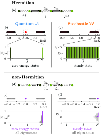
Figure 1: Non-Hermiticity is necessary for topological edge localization in stochastic systems. We contrast the behavior of Hermitian (top half) and non-Hermitian (bottom half) Su-Schriefer-Heeger (SSH) models [49, 50] describing quantum (left column) and stochastic (right column) systems. (a) Hermitian SSH model has reciprocal transition rates. (b) Top: spectrum of the quantum Hermitian topological model demonstrates two degenerate edge-localized states (red) inside the gap. These states are displayed in the bottom panel, with vector components colored as the corresponding sites. (c) On contrary, the spectrum of the stochastic Hermitian model, with the same topological invariant, has no edge-localized states, and the steady state presented in the bottom panel is homogeneous. Hence, Hermitian stochastic networks violate the bulk-edge correspondence. (d) Transition rates in the non-Hermitian SSH model are non-reciprocal. (e, f) Both quantum and stochastic non-Hermitian models have all eigenstates localized on the right edge. Localization is also present for the zero-energy quantum state (e) and stochastic steady state (f), highlighted with purple. All plots are made with open boundary conditions and panels (b, c) are plotted for $\gamma_{\textnormal{in}}=0.2$, $\gamma_{\textnormal{ex}}=0.8$, $N=20$, and panels (e, f) for $\gamma_{\textnormal{ex}}=0.64$, $\gamma_{\textnormal{ex}}^{\prime}=\gamma_{\textnormal{in}}=0.16$, $\gamma_{\textnormal{in}}^{\prime}=0.04$.

II Non-Hermiticity is necessary in stochastic models for topological edge localization

We study a stochastic system on a network, described by a master equation $\partial_{t}p=\mathcal{W}p$, where $p_{j}$ is the probability of finding the system at site $j$, and the transition rates from site $j$ to site $i$ form the transition matrix $\mathcal{W}_{ij}$. The master equation is similar to the Schrödinger equation of the quantum dynamics $i\partial_{t}\psi=\mathcal{H}\psi$: observe that one operator can be mapped onto the other using $\mathcal{H}=i\mathcal{W}$ [21, 20]. Since this mapping preserves the eigenvectors, topological invariants, that are defined in terms of eigenvectors of the quantum Hamiltonian $\mathcal{H}$ [1, 3], can also be defined for stochastic systems.

However, the same topological invariant can have different physical manifestations in quantum and stochastic systems. Topological invariants are typically computed under periodic boundary conditions (PBC). We consider quantum and stochastic networks with the same topological invariant, which is satisfied for regular networks, where the sum of outgoing rates from each site is the same across the whole network [51, 52, 36], $\sum_{i\neq j}\mathcal{W}_{ij}=\mathrm{Const}$ $\forall$ $j$. More precisely, to conserve the total probability over time, the stochastic transition matrix takes the form $\mathcal{W}=\mathcal{A}-\mathcal{D}$ [53]. Here, $\mathcal{A}_{ij}=\bra{i}\ket{j}$ describes the transition rates between different sites $i\neq j$, and the diagonal matrix $\mathcal{D}_{ij}=\delta_{ij}\sum_{k\neq j}\mathcal{A}_{kj}$ encodes the sum of the rates leaving each site. Both matrices are real and non-negative. We observe that the off-diagonal matrix $\mathcal{A}$ takes a similar form to a tight-binding Hamiltonian of a quantum system with the same network. In regular periodic networks the matrix $\mathcal{D}$ is proportional to the identity matrix, and hence the PBC spectra of $\mathcal{A}$ and $\mathcal{W}$ differ only by a constant shift. In this case, the quantum matrix $\mathcal{A}$ has the same eigenvectors as the stochastic matrix $\mathcal{W}$, and hence the same topological invariant.

Given that stochastic and quantum systems can share the same topological invariant under periodic boundary conditions, i.e. in the bulk, we examine how this invariant is reflected on the edge. We expect a bulk topological invariant to give rise to a physical response on the edge, due to the bulk-edge correspondence [32, 33, 34], a celebrated principle in quantum topological systems. We illustrate this principle using the 1D Su-Schrieffer-Heeger (SSH) model [49, 54] (see Fig. 1(a)), whose Hamiltonian under periodic boundary conditions is given by

$$\mathcal{A}(k)=\begin{pmatrix}0&\gamma_{\textnormal{in}}+\gamma_{\textnormal{ex}}e^{ik}\\ \gamma_{\textnormal{in}}+\gamma_{\textnormal{ex}}e^{-ik}&0\end{pmatrix}.$$ (1)

The alternating internal rates $\gamma_{\textnormal{in}}$ and external rates $\gamma_{\textnormal{ex}}$ determine the value of the Zak phase topological invariant [55, 56] (details in Appendix A.1), which is non-zero when $\gamma_{\textnormal{ex}}>\gamma_{\textnormal{in}}$. In this case, the zero-energy eigenstates are localized on the system edge (see Fig. 1(b)), as expected from the bulk-edge correspondence. We denote the eigenvalues and eigenstates of $\mathcal{A}$ with $E$ and $\psi$ respectively. Despite that the Zak phase topological invariant can be defined in both quantum and stochastic models, we find that the stochastic steady state is homogeneous without edge localization (see Fig. 1(c)), which appears to break the bulk-edge correspondence. We denote the eigenvalues and eigenstates of $\mathcal{W}$ with $E$ and $p$ respectively.

To understand why the bulk-edge correspondence has broken, we note two differences when considering quantum and stochastic systems. First, open boundaries cause the elements of the matrix $\mathcal{D}$ to vary, resulting in different quantum and stochastic open boundary spectra. As this difference is concentrated near the edge, it mostly affects the edge response of the stochastic system and can render it drastically different from the quantum system. Second, the typical states of interest in quantum and stochastic systems can be found in different regions of the spectrum. In the quantum case, the states near the Fermi energy are the most relevant, while in the stochastic case, it is the steady state $\bar{p}$ which satisfies $\mathcal{W}\bar{p}=0$. Each of these states is highlighted in Figs. 1(b) and (c) respectively, using a dashed rectangle. These differences contribute to the striking difference in edge response despite the same bulk invariant, that we saw previously.

We prove that the homogeneous steady state is a more general result that holds for networks of any geometry and dimension, so long as they are Hermitian (aka reciprocal). Combining probability conservation $\sum_{i}\mathcal{W}_{ij}=0$ with Hermiticity $\mathcal{W}_{ij}=\mathcal{W}_{ji}$, we obtain that the sum of rates leaving site $j$ is equal to the sum of rates arriving to this site $-\mathcal{W}_{jj}=\sum_{i\neq j}\mathcal{W}_{ji}$. Hence, equal probability on each site $\bar{p}_{i}=1/N$ will produce a zero net probability flow $\sum_{i}\mathcal{W}_{ji}\bar{p}_{i}=0$, i.e. the condition for the steady state. Since the steady state is unique according to the Perron–Frobenius theorem [57, 58], we have proved that the steady state is homogeneous in any reciprocal network.

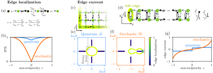
Figure 2: Edge localization grows dramatically with non-reciprocity in stochastic systems but plateaus in quantum systems. (a) In a non-Hermitian SSH chain, we reduce its parameter space to two parameters: ratio between external and internal rates $r=(\gamma_{\textnormal{ex}}-\gamma_{\textnormal{in}})/(\gamma_{\textnormal{ex}}+\gamma_{\textnormal{in}})$ and non-reciprocity or chirality $c$; the latter controls the strength of non-Hermiticity. (b) The inverse participation ratio (IPR) quantifies localization of the stochastic steady state (orange line) and the quantum zero-energy state (blue line). As the system transitions from the reciprocal $c=0$ to the fully non-reciprocal limit $c=\pm 1$, the IPR grows in the stochastic case but plateaus in the quantum case. (c) We verify that this effect also holds for an edge current in a 2D non-Hermitian SSH model [21]. (d) The fully finite network is approximated by a ribbon with open boundary condition along the $x$-axis and periodic boundary condition along the $y$-axis, described with external rates multiplied by $e^{\pm ik_{y}}$ (curved arrows). We focus on currents on the left edge of the ribbon (highlighted with yellow). (e) In the quantum spectrum, where shades of purple-to-yellow indicate degree of edge localization, the persistent current is calculated in the occupied state with the largest $\imaginary E$, indicated with a dashed rectangle for a system at $1/4$ filling. (f) In the stochastic spectrum, the current is calculated in the steady state (indicated with a dashed rectangle), that is a mixture of the bulk and edge-localized states. (g) Again, the stochastic edge current (orange) grows with non-reciprocity $c$, while the quantum current (blue) plateaus, just as in the 1D model. Panel (b) is plotted for $r=0.6$, panel (g) for $r=0.5$, panels (e, f) for $r=0.5$, $c=0.9$.

Seeing that Hermitian stochastic systems break the bulk-edge correspondence sheds light on why all stochastic topological models to date have needed non-reciprocity [21, 22, 19, 20]. Indeed, non-reciprocal transitions can restore edge-localization in the steady state as we show by going to the non-Hermitian SSH model (Fig. 1(d)), where we introduce the backward rates $\gamma_{\textnormal{in}}^{\prime}$ and $\gamma_{\textnormal{ex}}^{\prime}$ in addition to each forward rate $\gamma_{\textnormal{in}}$ and $\gamma_{\textnormal{ex}}$. Thus the quantum Hamiltonian under periodic boundary conditions takes the form

$$\mathcal{A}(k)=\begin{pmatrix}0&\gamma_{\textnormal{in}}^{\prime}+\gamma_{\textnormal{ex}}e^{ik}\\ \gamma_{\textnormal{in}}+\gamma_{\textnormal{ex}}^{\prime}e^{-ik}&0\end{pmatrix},$$ (2)

and the stochastic transition matrix on the same network acquires additional diagonal terms $\mathcal{D}=\mathrm{diag}(\gamma_{\textnormal{in}}+\gamma_{\textnormal{ex}}^{\prime},\gamma_{\textnormal{in}}^{\prime}+\gamma_{\textnormal{ex}})$.

To simplify the parameter space, we express the four rates in terms of two parameters and an overall scaling factor $\gamma_{\textnormal{in}}=\gamma_{\textnormal{tot}}(1-r)(1+c)/4$, $\gamma_{\textnormal{in}}^{\prime}=\gamma_{\textnormal{tot}}(1-r)(1-c)/4$, $\gamma_{\textnormal{ex}}=\gamma_{\textnormal{tot}}(1+r)(1+c)/4$ and $\gamma_{\textnormal{ex}}^{\prime}=\gamma_{\textnormal{tot}}(1+r)(1-c)/4$. The ratio $r$ determines the balance between external and internal rates, where $r=0$ is the transition between the topological and trivial phases in the Hermitian limit. The non-reciprocity $c$ determines the balance between forward and backward rates, where $c=0$ is the Hermitian limit and $c=\pm 1$ is fully chiral or non-Hermitian. When $c\neq 0$, both quantum and stochastic models carry the non-Hermitian topological invariant given by the spectral winding in the PBC spectrum [50, 59, 60, 61, 20] (details in App. A.2). In this regime, the zero-energy quantum state and the stochastic steady state, along with all the other states, become localized on the edge (Fig. 1(e, f)).

III Edge localization grows dramatically with non-reciprocity in stochastic systems but plateaus in quantum systems

Having seen that non-Hermiticity is necessary for stochastic edge states, we ask whether these states are similar to edge states in non-Hermitian quantum systems. To quantify a state localization we calculate its inverse participation ratio [62] as $\mathrm{IPR}(\psi)=\sum_{j=1}^{N}|\psi_{j}|^{4}/\bra{\psi}\ket{\psi}^{2}$. For the non-Hermitian SSH chain (Fig. 2(a)), we calculate the IPR for the quantum zero-energy state and the stochastic steady state as a function of non-reciprocity $c$ (see Appendix A.3 for derivation of IPR). We observe that in the quantum system, localization depends weakly on non-reciprocity, while in the stochastic system, it grows with non-reciprocity and peaks in a fully non-reciprocal chain at $c=\pm 1$ (Fig. 2(b)). To understand this behavior we note that in the Hermitian quantum model at $c=0$, the states are edge-localized due to the Zak phase. Therefore, the non-Hermitian spectral winding [59] modifies localization only weakly. In the stochastic case, we showed that there is no localization in the Hermitian limit and hence localization grows steadily as non-reciprocity increases.

However, we would like to understand if this different dependence on non-reciprocity in stochastic and quantum edge states holds more generally, i.e., outside of states with PBC spectral winding. Hence, we turn to a model with a qualitatively different physical response, that of edge currents [21, 22]. This is a 2D non-Hermitian SSH model with a similar rate parametrization (see Fig. 2(c) and Appendix B.1 for details). As the network is regular, both quantum and stochastic systems have the same topological invariant – the vectored Zak phase [63, 64]. To simplify the analysis, we approximate the model with all open boundaries by a ribbon with an open boundary condition in the $x$ direction and a periodic boundary condition in the $y$ direction, which guarantees a well-defined momentum $k_{y}$ (Fig. 2(d)). As we show in Appendix B.1, the fully open and the ribbon models have similar spectra for large enough systems. We study persistent currents flowing along the left edge of the ribbon.

Quantum and stochastic persistent currents originate from different areas of the spectrum. This demands different methods to calculate the current in each case, which we outline below. Quantum persistent current can only exist in a band with non-zero spectral winding, as argued in Ref. [43]. In such a band, two states with opposite group velocities $v_{g}=\partial_{k_{y}}\real E$ will have different imaginary energies, which determine their growth or decay rate during time evolution [65, 66, 67]. Therefore, at long timescales, the system develops a current, that is equal to the group velocity of the occupied state with the largest $\imaginary E$. In the 2D SSH model, the vectored Zak phase protects edge-localized bands inside the spectral gap [63, 64] (see Appendix B.2 for details). These bands acquire a spectral winding when transition rates become non-reciprocal $c\neq 0$ (see Fig. 2(e)). This spectrum is an example of a topologically protected edge spectral winding, discussed in Ref. [68]. Assuming that the quantum SSH model has one electron per unit cell, the persistent current is calculated in the state indicated with a dashed rectangle in Fig. 2(e). Note that edge localization is calculated as the sum over squared magnitudes for all vector components lying on the edge $\sum_{j\in\textnormal{edge}}|\psi_{j}|^{2}$.

In the stochastic model, the diagonal terms $\mathcal{D}=\mathcal{A}-\mathcal{W}$ shift the edge band such that it overlaps with the bulk. The steady state, indicated with a dashed rectangle in Fig. 2(f), is therefore a mixture of bulk distributed and edge localized probability. The persistent current is calculated as a steady state probability flow along the network edge [21] and has a non-zero contribution only from the edge localized portion of the steady state (see Appendix B.3 for details).

Having identified the quantum and stochastic persistent currents, we track in Fig. 2(g) how their values change with non-reciprocity $c$. Again, the stochastic current grows dramatically with non-reciprocity, while the quantum current plateaus, just as in the 1D model. These trends can be understood by observing that non-reciprocity mainly affects the imaginary component of the edge band, much more than the real component. As the quantum current depends on the momentum derivative of this real component, it is not strongly altered by non-reciprocity. Instead, the edge localized portion of the steady state grows with non-reciprocity [21], which strongly affects the stochastic current.

Interestingly, we have found that stochastic edge localization differs from quantum edge localization in a similar manner in both 1D and 2D systems (Figs. 2(b) and (g) respectively), despite that the physical mechanisms in each case are very different. We discuss the reasons for localization in both cases in the following section.

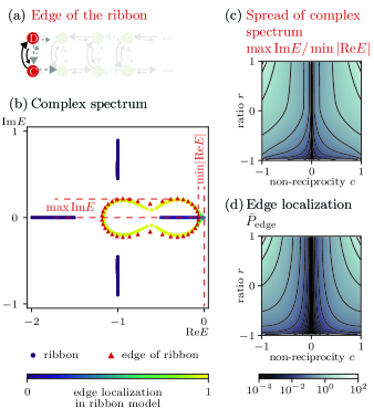
Figure 3: In stochastic systems, spread of the complex spectrum induces edge localization, which is necessary for the edge current. (a) To characterize the spread of the edge band, we introduce an auxiliary 1D model, that emulates the edge of the stochastic 2D SSH ribbon presented in Fig. 2(d). (b) To confirm that the two models are close, we plot the spectra of the 2D SSH model (purple vs. yellow dots denoting bulk distributed vs. edge localized states), and of the edge model (red triangles) at $r=0.5$ and $c=0.9$. We characterize the edge model spectrum by the largest imaginary component among all eigenvalues $\max\imaginary E$ and the smallest magnitude among all real components $\min|\real E|$. We observe that (c) the overall complex spread of the edge model, expressed as $\max\imaginary E/\min|\real E|$, is similar in shape to (d) total excess of probability on the edge of the 2D model $\bar{P}_{\textnormal{edge}}$. This similarity indicates that spread in the complex spectrum leads to edge localization and hence the steady-state current.

IV Non-reciprocity restores the bulk-edge correspondence in stochastic systems

We showed that in the 1D SSH chain, non-reciprocity localizes all eigenstates on one edge (Fig. 1(f)). Such behavior in quantum models has been attributed to the non-Hermitian skin effect [69, 41, 42, 70], and this skin effect is also likely responsible for localization in stochastic models [20]. However, in the 2D SSH model discussed above, the skin effect is absent as the bulk spectrum has zero spectral area [71]. How then does non-reciprocity produces edge currents in such systems without the skin effect? One clue comes from Fig. 2(f), where we see that the bulk (purple) and edge (yellow) states become hybridized (green) close to the steady state, in contrast to the quantum system in Fig. 2(e) where the bulk and edge states remain distinct. This suggests that hybridization is what prevents edge localization in the reciprocal case, even in the presence of a bulk topological invariant. Non-reciprocity may provide a mechanism to minimize such hybridization by causing the spectrum to become complex and allowing eigenvalues to spread out.

To investigate this, we quantify the complex shape of the edge band and compare it to the steady state localization. We note that directly characterizing the shape of the edge band is not possible as it mixes with the bulk band in the vicinity of the steady state. Hence, we introduce a 1D edge model that emulates the edge of the 2D model (see Fig. 3(a)). It consists of sites and transition rates that are closest to the edge of the 2D model, as well as the rates that go from the edge to the bulk ($\gamma_{\textnormal{in}}^{\prime}$ and $\gamma_{\textnormal{in}}$), as described by the transition matrix

$$\mathcal{W}_{\textnormal{1D edge}}=\begin{pmatrix}-\gamma_{\textnormal{in}}-\gamma_{\textnormal{in}}^{\prime}-\gamma_{\textnormal{ex}}^{\prime}&\gamma_{\textnormal{in}}^{\prime}+\gamma_{\textnormal{ex}}e^{ik}\\ \gamma_{\textnormal{in}}+\gamma_{\textnormal{ex}}^{\prime}e^{-ik}&-\gamma_{\textnormal{in}}-\gamma_{\textnormal{in}}^{\prime}-\gamma_{\textnormal{ex}}\end{pmatrix}.$$ (3)

The spectrum of the 1D edge model, shown in Fig. 3(b), overlaps with the edge-localized band of the 2D model in the topological phase (see Appendix B.4). We characterize the shape of this 1D edge spectrum by generalizing the ratio between imaginary and real components of the first non-zero eigenvalue, which is the coherence of stochastic oscillations [72]. Here, for the numerator we use the largest imaginary component among all eigenvalues $\max\imaginary E$, which quantifies the spread in imaginary space. For the denominator, we use the smallest magnitude among real components $\min|\real E|$, whose inverse $(\min|\real E|)^{-1}$ is the longest lifetime among all the modes. Hence, we use the ratio $\max\imaginary E/\min|\real E|$ as a measure of the spread of the complex spectrum weighted by its lifetime, which is plotted in Fig. 3(c).

We calculate the edge-localization in the 2D model as the total excess of probability on the edge over the homogeneous bulk value $\bar{P}_{\textnormal{edge}}=\sum_{i}(\bar{p}_{i}-\bar{p}_{\textnormal{bulk}})/\bar{p}_{\textnormal{bulk}}$ [21] (see Appendix B.3) and plot it in Fig. 3(d). We observe that the two quantities in Figs. 3(c) and (d) have a similar shape as a function of model parameters. They both grow from zero in the reciprocal limit $c=0$ to their peak values in the fully non-reciprocal limit $c=\pm 1$ and also grow with the ratio $r$. This suggests that the spread in the complex spectrum leads to edge localization by reducing hybridization between the edge and bulk eigenstates. Hence non-reciprocity, which allows edge states to be distinct from the bulk states in the complex plane, restores the bulk-edge correspondence even in the absence of the skin effect.

V Discussion

Our understanding of stochastic topological systems and their efficient use for biological applications requires the development of general theoretical principles for these systems. In this work, we laid the foundation for such principles by showing that stochastic topological systems require non-reciprocal transition rates for a robust edge response. Moreover, edge localization in stochastic networks grows with non-reciprocity, distinguishing them from quantum models defined on the same networks. Interestingly, such localization growth resembles a similar behavior in the quantum Hatano-Nelson model [73], and further study is necessary to refine the similarities and differences between non-reciprocal quantum and stochastic systems.

The necessity of a non-Hermitian description raises further questions about how various non-Hermitian phenomena affect the behavior of stochastic networks. While the non-Hermitian skin effect provides edge localization in a 1D stochastic system, future studies will show how multi-dimensional generalizations of the skin effect [74, 71, 75] help localization in a broader set of stochastic models. Furthermore, exceptional points, that are unique to non-Hermitian systems [45, 46, 48], were shown to protect edge-localized states in quantum and hydrodynamic materials [47]. Finding a stochastic system with exceptional points may realize a new mechanism of steady state localization. A more systematic approach to stochastic topological systems, similar to the topological classification of non-Hermitian quantum Hamiltonians in 38 symmetry classes [76, 45], requires further identification of possible symmetries in stochastic models and development of a complete topological classification for stochastic transition matrices. As stochastic models have to be real, the method of mapping complex-valued quantum dynamics to real-valued stochastic dynamics on an enlarged network [77] will open an avenue towards new stochastic topological phenomena.

Besides fundamental questions about stochastic topology, our work provides insights into biological applications. Stochastic networks are known to describe various processes in biological organisms, such as cyclic biochemical reactions [22] or signaling pathways [19]. Localized steady state in these networks restricts the system to a region of its configuration space where it performs a biological function [19]. We show that non-reciprocal transition rates are necessary for such localization and hence for stable functioning. It agrees with the fact that a system with reciprocal rates obeys the principle of microscopic reversibility and can not develop any asymmetry in information flow, as discussed in Ref. [78]. These results of specific and targeted responses that can be tuned by non-reciprocity provides design principles for synthetic biological systems with robust behavior [79, 80], such as biochemical oscillators [81, 82] or ring attractors [83, 84]. Overall, our work provides general principles towards our understanding of non-equilibrium systems and their robust function.

Appendix A Su-Schriefer-Heeger model

In this appendix, we provide more details about the 1D Su-Schriefer-Heeger (SSH) model and its topological classification. Section A.1 deals with the Hermitian model, while section A.2 with the non-Hermitian model. We derive the zero eigenstates of the non-Hermitian SSH model in section A.3.

A.1 Hermitian SSH model

Hermitian SSH model is shown in Fig. 1(a) in the main text. Due to translational symmetry, under periodic boundary conditions this model is described by a matrix defined over reciprocal space. The quantum Hamiltonian as a function of momentum $k\in[-\pi,\pi]$ is given by

$$\mathcal{A}=\begin{pmatrix}0&\gamma_{\textnormal{in}}+\gamma_{\textnormal{ex}}e^{ik}\\ \gamma_{\textnormal{in}}+\gamma_{\textnormal{ex}}e^{-ik}&0\end{pmatrix}.$$ (4)

The corresponding stochastic transition matrix includes additional diagonal terms that account for probability conservation:

$$\mathcal{W}=\begin{pmatrix}-\gamma_{\textnormal{in}}-\gamma_{\textnormal{ex}}&\gamma_{\textnormal{in}}+\gamma_{\textnormal{ex}}e^{ik}\\ \gamma_{\textnormal{in}}+\gamma_{\textnormal{ex}}e^{-ik}&-\gamma_{\textnormal{in}}-\gamma_{\textnormal{ex}}\end{pmatrix}.$$ (5)

With periodic boundary conditions, the quantum and stochastic matrices differ merely by a constant shift and therefore have the same topological classification. Namely, they exist in two different phases, determined by the Zak phase topological invariant [55, 56] protected by the inversion symmetry $\sigma_{x}\mathcal{M}(k)\sigma_{x}=\mathcal{M}(-k)$ for $\mathcal{M}=\mathcal{A},\mathcal{W}$. The Zak phase takes the form

$$\Phi=\int_{-\pi}^{\pi}dk\bra{\psi_{1}(k)}\partial_{k}\ket{\psi_{1}(k)}\in\{0,\pi\},$$ (6)

where $\ket{\psi_{1}(k)}$ is the eigenvector of both quantum $\mathcal{A}(k)$ and stochastic $\mathcal{W}(k)$ matrices, corresponding to the lower eigenvalue. The Zak phase is non-zero when $\gamma_{\textnormal{ex}}>\gamma_{\textnormal{in}}$.

In the main text we showed that under open boundary conditions, the quantum and stochastic models have different behavior: the quantum model has zero-energy eigenstates localized on the edge, while the stochastic steady state is homogeneously distributed over the bulk. In the main text, this result was proven generally for any Hermitian model. Here we provide an additional model-specific explanation for the absence of edge-localized stochastic modes. We know that the stochastic SSH model is different from the quantum SSH model by the diagonal terms $\mathcal{W}=\mathcal{A}-\mathcal{D}$. We notice that under open boundary conditions, the diagonal terms are decomposed into a constant diagonal and an edge-localized matrix $\mathcal{D}=(\gamma_{\textnormal{in}}+\gamma_{\textnormal{ex}})I-\mathcal{P}$. Here $I$ is the identity matrix and

$$\mathcal{P}_{ij,\alpha\beta}=(\delta_{i1}\delta_{j1}\delta_{\alpha 1}\delta_{\beta 1}+\delta_{iN}\delta_{jN}\delta_{\alpha 2}\delta_{\beta 2})\gamma_{\textnormal{ex}},$$ (7)

with $i,j=1,..N$ being unit cell indices and $\alpha,\beta=1,2$ indicating a site within the unit cell. The edge-localized term $\mathcal{P}$ breaks the sublattice symmetry $\sigma_{z}\mathcal{A}(k)\sigma_{z}=-\mathcal{A}(-k)$, which protects the zero-energy states in the quantum model [54]. Therefore, edge-localized states do not exist in the gap of the stochastic model due to the symmetry-breaking edge terms.

A.2 Non-Hermitian SSH model

The non-Hermitian SSH model is illustrated in Fig. 2(a) in the main text and generalizes the Hermitian SSH model by allowing non-reciprocal transition rates. The quantum model under periodic boundary conditions is given by

$$\mathcal{A}=\begin{pmatrix}0&\gamma_{\textnormal{in}}^{\prime}+\gamma_{\textnormal{ex}}e^{ik}\\ \gamma_{\textnormal{in}}+\gamma_{\textnormal{ex}}^{\prime}e^{-ik}&0\end{pmatrix}.$$ (8)

where $\gamma_{\textnormal{in}}^{\prime}$ and $\gamma_{\textnormal{ex}}^{\prime}$ are backwards rates corresponding to the forward rates $\gamma_{\textnormal{in}}$ and $\gamma_{\textnormal{ex}}$, respectively. The stochastic model is given by

$$\mathcal{W}=\begin{pmatrix}-\gamma_{\textnormal{in}}-\gamma_{\textnormal{ex}}^{\prime}&\gamma_{\textnormal{in}}^{\prime}+\gamma_{\textnormal{ex}}e^{ik}\\ \gamma_{\textnormal{in}}+\gamma_{\textnormal{ex}}^{\prime}e^{-ik}&-\gamma_{\textnormal{in}}^{\prime}-\gamma_{\textnormal{ex}}\end{pmatrix},$$ (9)

To reduce the parameter space, the four rates are parameterized using the overall scaling factor $\gamma_{\textnormal{tot}}$, ratio $r$ and non-reciprocity $c$:

$$\gamma_{\textnormal{ex}}=\gamma_{\textnormal{tot}}(1+c)(1+r)/4,$$

$$\gamma_{\textnormal{ex}}^{\prime}=\gamma_{\textnormal{tot}}(1-c)(1+r)/4,$$

$$\gamma_{\textnormal{in}}=\gamma_{\textnormal{tot}}(1+c)(1-r)/4,$$

$$\gamma_{\textnormal{in}}^{\prime}=\gamma_{\textnormal{tot}}(1-c)(1-r)/4.$$ (10)

Both the quantum and stochastic models possess a non-Hermitian topological invariant – the spectral winding number

$$\nu(E_{0})=\frac{1}{2\pi i}\int_{-\pi}^{\pi}\partial_{k}\log(\det(\mathcal{M}(k)-E_{0}))dk,$$ (11)

with $\mathcal{M}=\mathcal{A}$ in the quantum case and $\mathcal{M}=\mathcal{W}$ in the stochastic case. $E_{0}$ is a reference energy around which the spectrum winds. For all parameters away from $r=\pm 1$ or $c=0$, both quantum and stochastic bands produce a non-zero winding. This means that both systems exhibit the skin effect [42, 20] and have their states (including the zero-energy states) localized on one edge.

A.3 Zero eigenstates and inverse participation ratio

We proceed to derive the zero-energy eigenstates of the quantum and stochastic SSH models and compute their inverse participation ratio. We follow the formalism presented for the quantum SSH model in Ref. [60].

A.3.1 Quantum zero-energy eigenstates

First, consider the quantum model and reproduce the derivation from Ref. [60]. We represent the system in real space and write the wavefunctions in the basis of vectors $\ket{n}\otimes\ket{\xi}$, with $\ket{n}$ encoding a state in the $n$-th unit cell, and $\ket{\xi}=(\xi_{1},\xi_{2})^{T}$ specifying the state distribution over sublattice $1$ and $2$. The quantum SSH Hamiltonian in real space is given by

$$\hat{\mathcal{A}}= \sum_{n}\begin{pmatrix}0&\gamma_{\textnormal{in}}^{\prime}\\ \gamma_{\textnormal{in}}&0\end{pmatrix}\ket{n}\bra{n}$$

$$+\begin{pmatrix}0&\gamma_{\textnormal{ex}}\\ 0&0\end{pmatrix}\ket{n}\bra{n-1}+\begin{pmatrix}0&0\\ \gamma_{\textnormal{ex}}^{\prime}&0\end{pmatrix}\ket{n}\bra{n+1}$$ (12)

To focus on a single edge, we assume that the chain is semi-infinite with only left edge. We search for an edge-localized eigenstate using the ansatz

$$\ket{\psi_{l}}=\frac{1}{\mathcal{N}}\sum_{n=1}^{N}\beta^{n-1}\ket{n}\otimes\ket{\xi},$$ (13)

with the size of the system $N\to\infty$. This state is a zero-energy eigenstate of the Hamiltonian if $\mathcal{A}\ket{\psi_{l}}=0$. We also search for a corresponding right eigenstate $\mathcal{A}^{\dagger}\ket{\phi_{l}}=0$, using the ansztz

$$\ket{\phi_{l}}=\frac{1}{\mathcal{N}}\sum_{n=1}^{N}\beta^{\prime n-1}\ket{n}\otimes\ket{\xi}.$$ (14)

We require that the two states form a biorthogonal pair $\bra{\phi_{l}}\ket{\psi_{l}}=1$.

Substituting the anzatz (13) to the eigenstate equation, we get the following equation in the bulk of the chain

$$\begin{pmatrix}0&\gamma_{\textnormal{in}}^{\prime}+\gamma_{\textnormal{ex}}\beta^{-1}\\ \gamma_{\textnormal{in}}+\gamma_{\textnormal{ex}}^{\prime}\beta&0\end{pmatrix}\ket{\xi}=0.$$ (15)

On the left edge the same vector $\ket{\xi}$ must satisfy the boundary condition

$$\begin{pmatrix}0&\gamma_{\textnormal{in}}^{\prime}\\ \gamma_{\textnormal{in}}+\gamma_{\textnormal{ex}}^{\prime}\beta&0\end{pmatrix}\ket{\xi}=0.$$ (16)

These equations are solved by $\beta=-\gamma_{\textnormal{in}}/\gamma_{\textnormal{ex}}^{\prime}$ and $\ket{\xi}=(1,0)^{T}$. Similarly, from the right eigenstate equation we get $\beta^{\prime}=-\gamma_{\textnormal{in}}^{\prime}/\gamma_{\textnormal{ex}}$. Biorthogonality of the two states specifies the normalization factor to be $\mathcal{N}=\sqrt{(1-(\beta^{\prime}\beta)^{N})/(1-\beta^{\prime}\beta)}$. For the zero-energy state to exist in a semi-infinite chain, the normalization factor must be finite in the limit of $N\to\infty$, which is true if $|\beta\beta^{\prime}|<1$. The zero-energy state forms a decaying solution when $|\beta|<1$. Expressing the rates in terms of the ratio $r$ and non-reciprocity $c$, as in Eq. (10), the left-localized zero-energy state exists for $r>0$ (e.g. when external rates are larger than internal) and $r>c$.

Following the same procedure, we derive the right-localized zero-energy state in a semi-infinite chain with the right edge. It is given by

$$\ket{\psi_{r}}=\frac{1}{\mathcal{N}}\sum_{n=0}^{N-1}\beta^{\prime n}\ket{N-n}\otimes\ket{\xi^{\prime}},$$ (17)

with $\ket{\xi^{\prime}}=(0,1)^{T}$. This state exists and has a finite normalization factor $\mathcal{N}$ when $r>0$ and $r>-c$. In Fig. 4 we illustrate parameter regions, in which a semi-infinite model has a left- or right-localized eigenstate with green and purple filling, respectively.

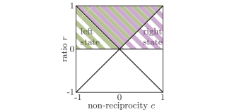
Figure 4: Green vs. purple filling indicates parameter values $c$ and $r$, for which left- vs. right-localized zero-energy state is present in a semi-infinite quantum SSH chain.

In a finite chain with both left and right edges, the eigenstates close to the zero energy are formed by a linear combination of right- and left-localized eigenstates [60]. The contribution of the right (left) eigenstate decays exponentially with the chain length $N$ for $c<0$ ($c>0$). Therefore, in the following we assume that when $c<0$, $r>0$ the model has a left-localized zero-energy state (13), and when $c>0$, $r>0$ a right-localized state (17). For $r<0$ no normalized zero-energy state can be found.

Next, to quantify the degree of localization of these states we compute their inverse participation ratio as defined in the main text

$$\mathrm{IPR}^{\mathrm{q}}_{l} =\frac{\sum_{j=1}^{N}|\psi_{l,j}|^{4}}{\bra{\psi_{l}}\ket{\psi_{l}}^{2}}$$

$$=\sum_{n=1}^{\infty}\frac{|\beta^{n-1}|^{4}}{\left(\sum_{n=1}^{\infty}|\beta^{n-1}|^{2}\right)^{2}}$$

$$=\frac{\left(1-(\gamma_{\textnormal{in}}/\gamma_{\textnormal{ex}}^{\prime})^{2}\right)^{2}}{1-(\gamma_{\textnormal{in}}/\gamma_{\textnormal{ex}}^{\prime})^{4}}$$

$$=\frac{(1-c)^{2}(1+r)^{2}-(1+c)^{2}(1-r)^{2}}{(1-c)^{2}(1+r)^{2}+(1+c)^{2}(1-r)^{2}}.$$ (18)

$$\mathrm{IPR}^{\mathrm{q}}_{r}=\dots=\frac{(1+c)^{2}(1+r)^{2}-(1-c)^{2}(1-r)^{2}}{(1+c)^{2}(1+r)^{2}+(1-c)^{2}(1-r)^{2}}.$$ (19)

We further define a directional inverse participation ratio (dIPR) whose sign indicates whether state is localized on the left or on the right

$$\mathrm{dIPR}=\begin{cases}-\mathrm{IPR}_{l},&c<0\\ \mathrm{IPR}_{r},&c>0\end{cases}$$ (20)

In Figure 5(a) we show dIPR for the full range of parameters $c$ and $r$.

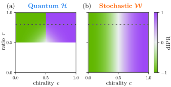
Figure 5: Directional inverse participation ratio in a long non-Hermitian SSH chain for a range of ratio $r$ and non-reciprocity $c$. (a) dIPR computed for the zero-energy quantum state. (b) dIPR computed for the stochastic steady state. Dashed line indicates the line, along which the inverse participation ratio is plotted in the main text in Fig. 2(b).

A.3.2 Stochastic steady state

We proceed to derive the steady state in the stochastic model. In real space, the transition matrix takes the form

$$\hat{\mathcal{W}}= \sum_{n}\begin{pmatrix}-\gamma_{\textnormal{in}}-\gamma_{\textnormal{ex}}^{\prime}&\gamma_{\textnormal{in}}^{\prime}\\ \gamma_{\textnormal{in}}&-\gamma_{\textnormal{in}}^{\prime}-\gamma_{\textnormal{ex}}\end{pmatrix}\ket{n}\bra{n}$$

$$+\begin{pmatrix}0&\gamma_{\textnormal{ex}}\\ 0&0\end{pmatrix}\ket{n}\bra{n-1}+\begin{pmatrix}0&0\\ \gamma_{\textnormal{ex}}^{\prime}&0\end{pmatrix}\ket{n}\bra{n+1}.$$ (21)

Similar to the quantum case, we search for a left-localized zero eigenstate of the transition matrix $\hat{\mathcal{W}}\ket{p_{l}}=0$ in the form

$$\ket{p_{l}}=\frac{1}{\mathcal{N}}\sum_{n=1}^{N}\delta^{n-1}\ket{n}\otimes\ket{\chi}$$ (22)

In the bulk this state must fulfill

$$\begin{pmatrix}-\gamma_{\textnormal{in}}-\gamma_{\textnormal{ex}}^{\prime}&\gamma_{\textnormal{in}}^{\prime}+\gamma_{\textnormal{ex}}\delta^{-1}\\ \gamma_{\textnormal{in}}+\gamma_{\textnormal{ex}}^{\prime}\delta&-\gamma_{\textnormal{in}}^{\prime}-\gamma_{\textnormal{ex}}\end{pmatrix}\ket{\chi}=0,$$ (23)

while the left boundary condition reads

$$\begin{pmatrix}-\gamma_{\textnormal{in}}&\gamma_{\textnormal{in}}^{\prime}\\ \gamma_{\textnormal{in}}+\gamma_{\textnormal{ex}}^{\prime}\delta&-\gamma_{\textnormal{in}}^{\prime}-\gamma_{\textnormal{ex}}\end{pmatrix}\ket{\chi}=0.$$ (24)

The state that satisfies this condition is given by $\delta=\gamma_{\textnormal{in}}\gamma_{\textnormal{ex}}/\gamma_{\textnormal{in}}^{\prime}\gamma_{\textnormal{ex}}^{\prime}$ and $\ket{\chi}=(\gamma_{\textnormal{in}}^{\prime},\gamma_{\textnormal{in}})^{T}$. This state decays from the left edge if $|\gamma_{\textnormal{in}}\gamma_{\textnormal{ex}}|<|\gamma_{\textnormal{in}}^{\prime}\gamma_{\textnormal{ex}}^{\prime}|$, which in terms of paramters $c$ and $r$ means $c<0$. Computing the corresponding right eigenvector $\mathcal{W}^{\dagger}\ket{p_{l}^{\prime}}=0$, we find that the binormalization factor $\mathcal{N}$ is finite for all $r\neq\pm 1$ and $c\neq 0$.

Similarly, the right-localized eigenstate can be found using the ansatz

$$\ket{p_{r}}=\frac{1}{\mathcal{N}}\sum_{n=0}^{N-1}\delta^{\prime n}\ket{N-n}\otimes\ket{\chi^{\prime}}.$$ (25)

Substituting it to the eigenstate equation we get $\delta^{\prime}=\delta^{-1}$ and $\ket{\chi^{\prime}}=\ket{\chi}$, which decays from the right edge when $c>0$.

Finally, we compute the IPR for these eigenstates. When $c<0$, IPR of the left-localized eigenstate is

$$\mathrm{IPR}_{l}^{\mathrm{st}} =\frac{\sum_{j=1}^{N}|p_{l,j}|^{4}}{\bra{p_{l}}\ket{p_{l}}^{2}}$$

$$=\sum_{n=1}^{\infty}\frac{|\delta^{n-1}|^{4}(|\chi_{1}|^{4}+|\chi_{2}|^{4})}{\left(\sum_{n=1}^{\infty}|\delta^{n-1}|^{2}(|\chi_{1}|^{2}+|\chi_{2}|^{2})\right)^{2}}$$

$$=\frac{((1-c)^{4}+(1+c)^{4})\left(1-(1+c)^{4}/(1-c)^{4}\right)^{2}}{((1-c)^{2}+(1+c)^{2})^{2}\left(1-(1+c)^{8}/(1-c)^{8}\right)}$$

$$=\frac{(1-c)^{2}-(1+c)^{2}}{(1-c)^{2}+(1+c)^{2}}=-\frac{2c}{1+c^{2}}.$$ (26)

Similarly, when $c>0$, the IPR of the right localized eigenstate is

$$\mathrm{IPR}_{r}^{\mathrm{st}}=\frac{2c}{1+c^{2}}.$$ (27)

We plot the corresponding dIPR for a range of parameters $c$ and $r$ in Fig. 5(b). In the main text, the absolute value of dIPR for the quantum and stochastic models is shown along a one-dimensional cut $r=0.6$, indicated with a dashed line in Fig. 5(a) and (b).

Appendix B 2D SSH model

In this Appendix, we provide more details about the 2D non-Hermitian Su-Schrieffer-Heeger model. In Sec. B.1 we specify the quantum Hamiltonian and the stochastic transition matrix. We discuss their topological classification in Sec. B.2. In Sec. B.3, we introduce the stochastic steady state probability and the edge current in a ribbon geometry. Finally, in Sec. B.4, we describe the 1D edge model that emulates the edge of the 2D model.

B.1 Transition matrices

The 2D SSH network [21] is shown in Fig. 2(d) and consists of four sites per unit cell. The sites are connected by internal transition rates $\gamma_{\textnormal{in}}$, which form a unidirectional cycle. Each forward rate is complemented with the corresponding backward rate $\gamma_{\textnormal{in}}^{\prime}$. The unit cells are connected by external transition rates $\gamma_{\textnormal{ex}}$, that form a cycle in the opposite direction with respect to the internal cycle. The corresponding backward rates are $\gamma_{\textnormal{ex}}^{\prime}$. In momentum space, the quantum 2D SSH model is described by the following Hamiltonian

$$\mathcal{A}= \left(\begin{matrix}0&\gamma_{\textnormal{in}}+\gamma^{\prime}_{\textnormal{ex}}e^{-ik_{y}}\\ \gamma^{\prime}_{\textnormal{in}}+\gamma_{\textnormal{ex}}e^{ik_{y}}&0\\ 0&\gamma^{\prime}_{\textnormal{in}}+\gamma_{\textnormal{ex}}e^{ik_{x}}\\ \gamma_{\textnormal{in}}+\gamma^{\prime}_{\textnormal{ex}}e^{ik_{x}}&0\end{matrix}\right.$$ (28)

$$\qquad\qquad\left.\begin{matrix}0&\gamma^{\prime}_{\textnormal{in}}+\gamma_{\textnormal{ex}}e^{-ik_{x}}\\ \gamma_{\textnormal{in}}+\gamma^{\prime}_{\textnormal{ex}}e^{-ik_{x}}&0\\ 0&\gamma_{\textnormal{in}}+\gamma^{\prime}_{\textnormal{ex}}e^{ik_{y}}\\ \gamma^{\prime}_{\textnormal{in}}+\gamma_{\textnormal{ex}}e^{-ik_{y}}&0\end{matrix}\right).$$

The stochastic transition matrix on the same network is given by

$$\mathcal{W}=\mathcal{A}-\gamma_{\textnormal{tot}}I,$$ (29)

where $I$ is the identity matrix, and $\gamma_{\textnormal{tot}}=\gamma_{\textnormal{in}}+\gamma_{\textnormal{in}}^{\prime}+\gamma_{\textnormal{ex}}+\gamma_{\textnormal{ex}}^{\prime}$. The second term ensures probability conservation in the stochastic model. In the following we assume the transition rates to be parameterized by non-reciprocity $c$ and ratio $r$, as in Eq. (10).

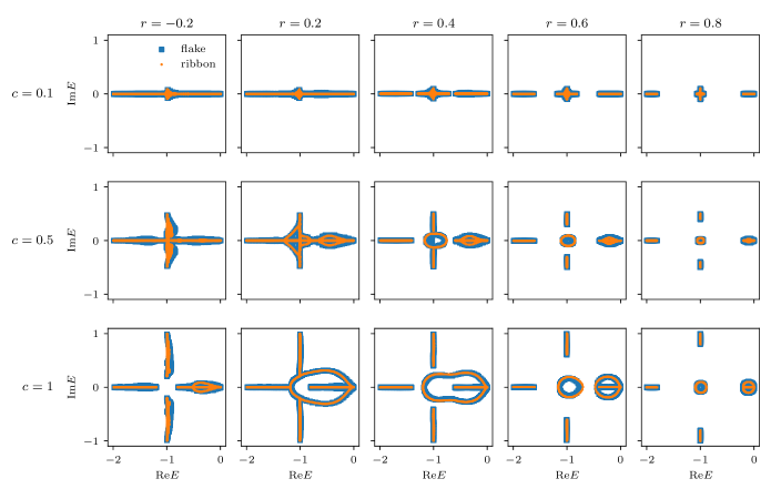
Figure 6: Comparison of the 2D SSH spectrum in the flake geometry with all open boundaries (blue squares) and in the ribbon geometry with periodic boundary condition along the $y$-axis (orange dots) for a number of model parameters $c$ and $r$. The spectra are similar, indicating that the ribbon geometry is a good approximation for a fully open system.

In the main text, we study how this model behaves on the edge. We stated that a model with open boundary conditions in both $x$ and $y$ directions can be approximated with a model in ribbon geometry with periodic boundary conditions in the $y$ direction. To justify this approximation, we plot in Fig. 6 the spectra of the fully open model (with blue squares) and the ribbon model (with orange dots) for a range of parameters $c$ and $r$. All models have 10 unit cells in the directions with open boundary conditions. We observe that the spectra of these models are close to each other, justifying our approximation.

B.2 Topological classification

In this section, we discuss topological invariants in the 2D SSH model. We start from the Hermitian case, when the rates are reciprocal $c=0$, and follow Ref. [63, 64] to characterize the topology of our model with a vectored Zak phase $\bm{\phi}=(\phi_{x},\phi_{y})$

$$\phi_{x} =\int_{-\pi}^{\pi}dk_{x}\bra{\psi_{1}(\bm{k})}\partial_{k_{x}}\ket{\psi_{1}(\bm{k})}\in\{0,\pi\},$$ (30)

$$\phi_{y} =\int_{-\pi}^{\pi}dk_{y}\bra{\psi_{1}(\bm{k})}\partial_{k_{y}}\ket{\psi_{1}(\bm{k})}\in\{0,\pi\},$$ (31)

where $\ket{\psi_{1}(\bm{k})}$ is the lowest eigenvector of both the quantum and the stochastic matrix. For external rates being larger than internal rates $r>0$, the model is in a topological phase with $\bm{\phi}=(\pi,\pi)$. When moving away from the Hermitian limit $c\neq 0$, the band structure becomes complex, as illustrated in Fig. 2(e) of the main text for parameters $c=0.9$, $r=0.5$. If the absolute value of ratio remains larger than the critical value $|r|>r^{*}(c)$ [21], the gap between the lower and the middle bulk bands remains open, and the system stays in the same topological phase as the Hermitian model.

We further discuss how this topological phase manifests on the edge of the quantum 2D SSH model. The Zak phase causes edge-localized states inside of the bulk gap. In the Hermitian limit, stability of these edge states was analyzed in Ref. [63], which stated that the edge states remain inside of the gap for perturbations with magnitude smaller than the gap size. Non-reciprocal rates cause the edge states to have a spectral winding, which is demonstrated for the left-localized band in Fig. 7, with momentum $k_{y}$ indicated by color to help visualizing the spectral winding. The winding number around the zero energy amounts to $\nu(E=0)=-1$. The right-localized bands are degenerate with the left-localized bands and have the opposite winding, as shown in the inset of Fig. 7. As discussed in the main text, the winding of the edge bands leads to persistent currents on the edge of the quantum model. We plot this current for the full range of parameters $r$ and $c$, at which the model is in the insulating phase (Fig. 8(a)). The critical ratio $\pm r^{*}(c)$, at which the model transitions to a semimetal is shown with a gray line.

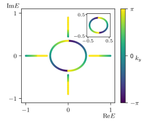
Figure 7: Spectrum of the quantum 2D non-Hermitian SSH ribbon with color denoting momentum $k_{y}$ of each eigenenergy. Momentum resolution helps to clearly see the winding of the edge bands in the middle. The main figure shows the left-localized band, while the right-localized band is shown in the inset and winds in the opposite direction. The plot is made at $r=0.9$ and $c=0.5$.

B.3 Stochastic edge observables

In this section, we summarize the edge quantities computed in the stochastic 2D SSH model: the steady state probability and the edge-localized current. These quantities were derived in Ref. [21] in Appendix D using the transfer matrix formalism, while here we reproduce the results.

The transfer matrix that acts on the probability vector in the $n$-th unit cell $[p_{D}^{n},p_{C}^{n},p_{A}^{n}.p_{B}^{n}]$ is given by

$$M =\begin{pmatrix}U_{1}&U_{2}\\ U_{4}U_{1}&U_{4}U_{2}+U_{3}\end{pmatrix},$$ (32)

$$U_{1} =\begin{pmatrix}-\gamma_{\textnormal{in}}^{\prime}/\gamma_{\textnormal{ex}}&0\\ 0&-\gamma_{\textnormal{in}}/\gamma_{\textnormal{ex}}^{\prime}\end{pmatrix},$$

$$U_{2} =\begin{pmatrix}\frac{\gamma_{\textnormal{in}}+\gamma_{\textnormal{ex}}+\gamma_{\textnormal{in}}^{\prime}+\gamma_{\textnormal{ex}}^{\prime}}{\gamma_{\textnormal{ex}}}&-\frac{\gamma_{\textnormal{in}}+\gamma_{\textnormal{ex}}^{\prime}}{\gamma_{\textnormal{ex}}}\\[5.69046pt] -\frac{\gamma_{\textnormal{in}}^{\prime}+\gamma_{\textnormal{ex}}}{\gamma_{\textnormal{ex}}^{\prime}}&\frac{\gamma_{\textnormal{in}}+\gamma_{\textnormal{ex}}+\gamma_{\textnormal{in}}^{\prime}+\gamma_{\textnormal{ex}}^{\prime}}{\gamma_{\textnormal{ex}}^{\prime}}\end{pmatrix},$$

$$U_{3} =\begin{pmatrix}-\gamma_{\textnormal{ex}}^{\prime}/\gamma_{\textnormal{in}}&0\\ 0&-\gamma_{\textnormal{ex}}/\gamma_{\textnormal{in}}^{\prime}\end{pmatrix},$$

$$U_{4} =\begin{pmatrix}\frac{\gamma_{\textnormal{in}}+\gamma_{\textnormal{ex}}+\gamma_{\textnormal{in}}^{\prime}+\gamma_{\textnormal{ex}}^{\prime}}{\gamma_{\textnormal{in}}}&-\frac{\gamma_{\textnormal{in}}^{\prime}+\gamma_{\textnormal{ex}}}{\gamma_{\textnormal{in}}}\\[5.69046pt] -\frac{\gamma_{\textnormal{in}}+\gamma_{\textnormal{ex}}^{\prime}}{\gamma_{\textnormal{in}}^{\prime}}&\frac{\gamma_{\textnormal{in}}+\gamma_{\textnormal{ex}}+\gamma_{\textnormal{in}}^{\prime}+\gamma_{\textnormal{ex}}^{\prime}}{\gamma_{\textnormal{in}}^{\prime}}\end{pmatrix}.$$ (33)

The transfer matrix has four eigenvectors corresponding to the steady state. Two of them are homogeneously distributed $\bm{V}_{1}=[1,1,1,1]^{T}$. One eigenvector is localized on the left edge $\bm{V}_{\alpha}$ with a decay constant given by the transfer matrix eigenvalue $\alpha$, while another is localized on the right with the same decay length. On the left edge, the following linear combination satisfies the boundary conditions:

$$\bm{P}_{0}=\bar{p}_{\textnormal{bulk}}(\bm{V}_{1}+\xi\bm{V}_{\alpha}),$$ (34)

where $\bar{p}_{\textnormal{bulk}}$ is the probability value in the bulk and $\xi$ is determined from the boundary conditions. Away from the left edge, the bulk portion of probability remains constant, while the edge-localized portion decays with the exponent $\alpha$. Then the steady state near the left edge is given by

$$\ket{\bar{p}}=\bar{p}_{\textnormal{bulk}}\sum_{n=0}(\bm{V}_{1}+\alpha^{n}\xi\bm{V}_{\alpha})\otimes\ket{n}.$$ (35)

Here, $\ket{n}$ encodes a state in the $n$-th unit cell along the $x$ direction. In the main text, we analyze edge-localization in the 2D SSH model by computing the total excess of probability on the edge over the homogeneous bulk value

$$\bar{P}_{\textnormal{edge}} =\sum_{i}(\bar{p}_{i}-\bar{p}_{\textnormal{bulk}})/\bar{p}_{\textnormal{bulk}}$$

$$=\sum_{n=0}\alpha^{n}\xi[1,1,1,1]\cdot\bm{V}_{\alpha}$$

$$=\frac{\xi}{1-\alpha}[1,1,1,1]\cdot\bm{V}_{\alpha}.$$ (36)

This quantity is plotted in Fig. 3(d).

In the steady state given by Eq. 35, the probability flow along the left edge is computed as

$$J_{\textnormal{st.}} =\sum_{n=0}[\gamma_{\textnormal{in}},-\gamma_{\textnormal{in}}^{\prime},\gamma_{\textnormal{in}}^{\prime},-\gamma_{\textnormal{in}}]\cdot\ket{\bar{p}}_{n},$$

$$=\bar{p}_{\textnormal{bulk}}\frac{\xi}{1-\alpha}[\gamma_{\textnormal{in}},-\gamma_{\textnormal{in}}^{\prime},\gamma_{\textnormal{in}}^{\prime},-\gamma_{\textnormal{in}}]\cdot\bm{V}_{\alpha}.$$ (37)

The edge-localized current is plotted in Fig. 2(g) in the units of $\bar{p}_{\textnormal{bulk}}\cdot\gamma_{\textnormal{tot}}$ as a function of non-reciprocity $c$. Stochastic edge current for the full range of ratio $r$ and non-reciprocity $c$ is plotted in Fig. 8(b).

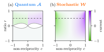
Figure 8: Persistent current flowing along the edge of the 2D SSH model as a function of ratio $r$ and non-reciprocity $c$. (a) The quantum current is computed as the group velocity of the state with the largest imaginary energy at quarter filling. Gray lines show the phase transition from an insulating to a semimetal phase. The current is calculated only in the insulating phase. (b) The stochastic current is computed using Eq. 37 and is shown in the units of $\bar{p}_{\textnormal{bulk}}\cdot\gamma_{\textnormal{tot}}$. The dashed line indicates parameter values at which the currents are plotted in Fig. 2(g) in the main text.

B.4 1D edge model

In this section, we provide more details about the 1D edge model, emulating the edge of the 2D SSH model in the ribbon geometry. Its transition matrix reads

$$\mathcal{W}_{\textnormal{1D edge}}=\begin{pmatrix}-\gamma_{\textnormal{in}}-\gamma_{\textnormal{in}}^{\prime}-\gamma_{\textnormal{ex}}^{\prime}&\gamma_{\textnormal{in}}^{\prime}+\gamma_{\textnormal{ex}}e^{ik}\\ \gamma_{\textnormal{in}}+\gamma_{\textnormal{ex}}^{\prime}e^{-ik}&-\gamma_{\textnormal{in}}-\gamma_{\textnormal{in}}^{\prime}-\gamma_{\textnormal{ex}}\end{pmatrix}.$$ (38)

We show the similarity between the spectrum of the 1D edge model and the edge-localized band of the 2D spectrum for a number of parameters in Fig. 9. Note that the 1D edge model does not conserve probability and hence does not necessarily have the steady state. We observe that deep in the topological phase when $r>r^{*}$, the two spectra are similar, making the 1D edge model a good approximation of the 2D edge band. Close to the phase transition and in the trivial phase $r\leq r^{*}$, the 1D edge model does not resemble the edge band of the 2D model. However, even in this regime, the complex spread of the 1D edge spectrum $\max\imaginary E/\min|\real E|$ resembles the 2D edge localization $\bar{P}_{\textnormal{edge}}$ (Fig. 3(c) vs (d)). To understand this, note that in the trivial phase the 2D localization vanishes, but so does the lifetime $(\min|\real E|)^{-1}$ of the 1D edge model, and hence the two functions still have a similar shape.

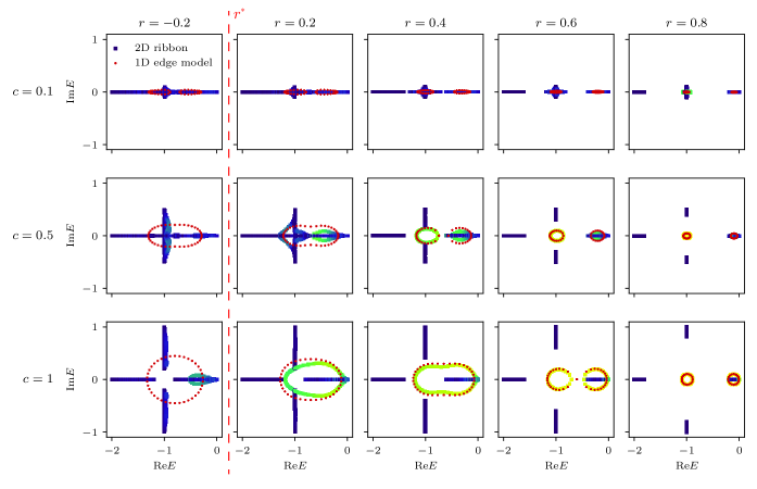
Figure 9: Comparison of the 2D SSH spectrum (purple-to-yellow squares) and the 1D edge model spectrum (red dots) for a number of model parameters $c$ and $r$. The edge-localized band of the 2D model (yellow color) can be approximated with the 1D edge model when the system is deep in the topological phase ($r>r^{*}$). The critical value $r^{*}$ with respect to the presented ratios $r$ is shown with a red dashed line.

References

- Hasan and Kane [2010] M. Z. Hasan and C. L. Kane, Colloquium : Topological insulators, Reviews of Modern Physics 82, 3045 (2010).
- Qi and Zhang [2011] X.-L. Qi and S.-C. Zhang, Topological insulators and superconductors, Reviews of Modern Physics 83, 1057 (2011).
- Bansil et al. [2016] A. Bansil, H. Lin, and T. Das, Colloquium : Topological band theory, Reviews of Modern Physics 88, 021004 (2016).
- Lu et al. [2014] L. Lu, J. D. Joannopoulos, and M. Soljačić, Topological photonics, Nature Photonics 8, 821 (2014).
- Ozawa et al. [2019] T. Ozawa, H. M. Price, A. Amo, N. Goldman, M. Hafezi, L. Lu, M. C. Rechtsman, D. Schuster, J. Simon, O. Zilberberg, and I. Carusotto, Topological photonics, Reviews of Modern Physics 91, 015006 (2019).
- Tang et al. [2022] G. Tang, X. He, F. Shi, J. Liu, X. Chen, and J. Dong, Topological Photonic Crystals: Physics, Designs, and Applications, Laser & Photonics Reviews 16, 2100300 (2022).
- Ma et al. [2019] G. Ma, M. Xiao, and C. T. Chan, Topological phases in acoustic and mechanical systems, Nature Reviews Physics 1, 281 (2019).
- Xue et al. [2022] H. Xue, Y. Yang, and B. Zhang, Topological acoustics, Nature Reviews Materials 7, 974 (2022).
- Mao and Lubensky [2018] X. Mao and T. C. Lubensky, Maxwell Lattices and Topological Mechanics, Annual Review of Condensed Matter Physics 9, 413 (2018).
- Zheng et al. [2022] S. Zheng, G. Duan, and B. Xia, Progress in Topological Mechanics, Applied Sciences 12, 1987 (2022).
- Lee et al. [2018] C. H. Lee, S. Imhof, C. Berger, F. Bayer, J. Brehm, L. W. Molenkamp, T. Kiessling, and R. Thomale, Topolectrical Circuits, Communications Physics 1, 39 (2018).
- Imhof et al. [2018] S. Imhof, C. Berger, F. Bayer, J. Brehm, L. W. Molenkamp, T. Kiessling, F. Schindler, C. H. Lee, M. Greiter, T. Neupert, and R. Thomale, Topolectrical-circuit realization of topological corner modes, Nature Physics 14, 925 (2018).
- Hofmann et al. [2019] T. Hofmann, T. Helbig, C. H. Lee, M. Greiter, and R. Thomale, Chiral Voltage Propagation and Calibration in a Topolectrical Chern Circuit, Physical Review Letters 122, 247702 (2019).
- Shankar et al. [2017] S. Shankar, M. J. Bowick, and M. C. Marchetti, Topological Sound and Flocking on Curved Surfaces, Physical Review X 7, 031039 (2017).
- Dasbiswas et al. [2018] K. Dasbiswas, K. K. Mandadapu, and S. Vaikuntanathan, Topological localization in out-of-equilibrium dissipative systems, Proceedings of the National Academy of Sciences 115, 10.1073/pnas.1721096115 (2018).
- Shankar et al. [2022] S. Shankar, A. Souslov, M. J. Bowick, M. C. Marchetti, and V. Vitelli, Topological active matter, Nature Reviews Physics 4, 380 (2022).
- Knebel et al. [2020] J. Knebel, P. M. Geiger, and E. Frey, Topological Phase Transition in Coupled Rock-Paper-Scissors Cycles, Physical Review Letters 125, 258301 (2020).
- Yoshida et al. [2021] T. Yoshida, T. Mizoguchi, and Y. Hatsugai, Chiral edge modes in evolutionary game theory: A kagome network of rock-paper-scissors cycles, Physical Review E 104, 025003 (2021).
- Murugan and Vaikuntanathan [2017] A. Murugan and S. Vaikuntanathan, Topologically protected modes in non-equilibrium stochastic systems, Nature Communications 8, 13881 (2017).
- Sawada et al. [2023] T. Sawada, K. Sone, Y. Ashida, and T. Sagawa, Role of Topology in Relaxation of One-dimensional Stochastic Processes (2023), arXiv:2301.09832 [cond-mat].
- Tang et al. [2021] E. Tang, J. Agudo-Canalejo, and R. Golestanian, Topology Protects Chiral Edge Currents in Stochastic Systems, Physical Review X 11, 031015 (2021).
- Zheng and Tang [2023] C. Zheng and E. Tang, A topological mechanism for robust and efficient global oscillations in biological networks (2023), arXiv:2302.11503 [cond-mat, physics:physics].
- Reid [1953] A. T. Reid, On Stochastic Processes in Biology, Biometrics 9, 275 (1953).
- Allen [2010] L. J. S. Allen, An Introduction to Stochastic Processes with Applications to Biology, 0th ed. (Chapman and Hall/CRC, 2010).
- Hahl and Kremling [2016] S. K. Hahl and A. Kremling, A Comparison of Deterministic and Stochastic Modeling Approaches for Biochemical Reaction Systems: On Fixed Points, Means, and Modes, Frontiers in Genetics 7, 10.3389/fgene.2016.00157 (2016).
- Hespanha and Khammash [2020] J. P. Hespanha and M. Khammash, Stochastic Description of Biochemical Networks, in Encyclopedia of Systems and Control, edited by J. Baillieul and T. Samad (Springer London, London, 2020) p. 2160.
- Qian and Ge [2021] H. Qian and H. Ge, Stochastic Chemical Reaction Systems in Biology (Springer, 2021).
- Barkai and Leibler [1997] N. Barkai and S. Leibler, Robustness in simple biochemical networks, Nature 387, 913 (1997).
- Kitano [2004] H. Kitano, Biological robustness, Nature Reviews Genetics 5, 826 (2004).
- Blanchini and Franco [2011] F. Blanchini and E. Franco, Structurally robust biological networks, BMC Systems Biology 5, 74 (2011).
- Félix and Barkoulas [2015] M.-A. Félix and M. Barkoulas, Pervasive robustness in biological systems, Nature Reviews Genetics 16, 483 (2015).
- Haldane [1988] F. D. M. Haldane, Model for a Quantum Hall Effect without Landau Levels: Condensed-Matter Realization of the ”Parity Anomaly”, Physical Review Letters 61, 2015 (1988).
- Kane and Mele [2005] C. L. Kane and E. J. Mele, Z 2 Topological Order and the Quantum Spin Hall Effect, Physical Review Letters 95, 10.1103/PhysRevLett.95.146802 (2005).
- Rhim et al. [2018] J.-W. Rhim, J. H. Bardarson, and R.-J. Slager, Unified bulk-boundary correspondence for band insulators, Physical Review B 97, 115143 (2018).
- Newman [2018] M. Newman, Networks (OUP Oxford, 2018).
- Wong et al. [2016] T. G. Wong, L. Tarrataca, and N. Nahimov, Laplacian versus adjacency matrix in quantum walk search, Quantum Information Processing 15, 4029 (2016).
- Mirzaev and Gunawardena [2013] I. Mirzaev and J. Gunawardena, Laplacian Dynamics on General Graphs, Bulletin of Mathematical Biology 75, 2118 (2013).
- Ashida et al. [2020] Y. Ashida, Z. Gong, and M. Ueda, Non-Hermitian physics, Advances in Physics 69, 249 (2020).
- Hosaka and Komura [2022] Y. Hosaka and S. Komura, Nonequilibrium Transport Induced by Biological Nanomachines, Biophysical Reviews and Letters 17, 51 (2022).
- Yao and Wang [2018] S. Yao and Z. Wang, Edge States and Topological Invariants of Non-Hermitian Systems, Physical Review Letters 121, 086803 (2018).
- Borgnia et al. [2020] D. S. Borgnia, A. J. Kruchkov, and R.-J. Slager, Non-Hermitian Boundary Modes and Topology, Physical Review Letters 124, 056802 (2020).
- Okuma et al. [2020] N. Okuma, K. Kawabata, K. Shiozaki, and M. Sato, Topological Origin of Non-Hermitian Skin Effects, Physical Review Letters 124, 086801 (2020).
- Zhang et al. [2020] K. Zhang, Z. Yang, and C. Fang, Correspondence between Winding Numbers and Skin Modes in Non-Hermitian Systems, Physical Review Letters 125, 126402 (2020).
- Zhang et al. [2022a] X. Zhang, T. Zhang, M.-H. Lu, and Y.-F. Chen, A review on non-Hermitian skin effect, Advances in Physics: X 7, 2109431 (2022a).
- Kawabata et al. [2019a] K. Kawabata, T. Bessho, and M. Sato, Classification of Exceptional Points and Non-Hermitian Topological Semimetals, Physical Review Letters 123, 066405 (2019a).
- Ding et al. [2022] K. Ding, C. Fang, and G. Ma, Non-Hermitian topology and exceptional-point geometries, Nature Reviews Physics 4, 745 (2022).
- Sone et al. [2020] K. Sone, Y. Ashida, and T. Sagawa, Exceptional non-Hermitian topological edge mode and its application to active matter, Nature Communications 11, 5745 (2020).
- Heiss [2012] W. D. Heiss, The physics of exceptional points, Journal of Physics A: Mathematical and Theoretical 45, 444016 (2012).
- Su et al. [1980] W. Su, J. R. Schrieffer, and A. J. Heeger, Soliton Excitations in Polyacetylene, Physical Review B 22, 2099 (1980).
- Lieu [2018] S. Lieu, Topological phases in the non-Hermitian Su-Schrieffer-Heeger model, Physical Review B 97, 045106 (2018).
- Chartrand [1977] G. Chartrand, Introductory Graph Theory (Dover: New York, 1977).
- Childs and Goldstone [2004] A. M. Childs and J. Goldstone, Spatial search by quantum walk, Physical Review A 70, 022314 (2004).
- Schnakenberg [1976] J. Schnakenberg, Network theory of microscopic and macroscopic behavior of master equation systems, Reviews of Modern Physics 48, 571 (1976).
- Asbóth et al. [2016] J. K. Asbóth, L. Oroszlány, and A. Pályi, A short course on topological insulators: band structure and edge states in one and two dimensions, Lecture notes in physics No. volume 919 (Springer, Cham Heidelberg New York Dordrecht London, 2016) oCLC: 942849465.
- Berry [1983] M. V. Berry, Quantal phase factors accompanying adiabatic changes, Proceedings of the Royal Society A 392, 45 (1983).
- Zak [1989] J. Zak, Berry’s phase for energy bands in solids, Physical Review Letters 62, 2747 (1989).
- Perron [1907] O. Perron, Zur Theorie der Matrices, Mathematische Annalen 64, 248 (1907).
- Frobenius [1912] G. Frobenius, Ueber Matrizen aus nicht negativen Elementen, Sitzungsberichte der Koeniglich Preussischen Akademie der Wissenschaften 26, 456 (1912).
- Yin et al. [2018] C. Yin, H. Jiang, L. Li, R. Lü, and S. Chen, Geometrical meaning of winding number and its characterization of topological phases in one-dimensional chiral non-Hermitian systems, Physical Review A 97, 052115 (2018).
- Jiang et al. [2020] H. Jiang, R. Lü, and S. Chen, Topological invariants, zero mode edge states and finite size effect for a generalized non-reciprocal Su-Schrieffer-Heeger model, The European Physical Journal B 93, 125 (2020).
- Zhu et al. [2021] W. Zhu, W. X. Teo, L. Li, and J. Gong, Delocalization of topological edge states, Physical Review B 103, 195414 (2021).
- Thouless [1974] D. Thouless, Electrons in disordered systems and the theory of localization, Physics Reports 13, 93 (1974).
- Liu and Wakabayashi [2017] F. Liu and K. Wakabayashi, Novel Topological Phase with a Zero Berry Curvature, Physical Review Letters 118, 076803 (2017).
- Obana et al. [2019] D. Obana, F. Liu, and K. Wakabayashi, Topological edge states in the Su-Schrieffer-Heeger model, Physical Review B 100, 075437 (2019).
- Lee et al. [2019] J. Y. Lee, J. Ahn, H. Zhou, and A. Vishwanath, Topological Correspondence between Hermitian and Non-Hermitian Systems: Anomalous Dynamics, Physical Review Letters 123, 206404 (2019).
- Longhi [2022] S. Longhi, Non-Hermitian skin effect and self-acceleration, Physical Review B 105, 245143 (2022).
- Kawabata et al. [2023] K. Kawabata, T. Numasawa, and S. Ryu, Entanglement Phase Transition Induced by the Non-Hermitian Skin Effect, Physical Review X 13, 021007 (2023), arXiv:2206.05384 [cond-mat, physics:quant-ph].
- Ou et al. [2023] Z. Ou, Y. Wang, and L. Li, Non-Hermitian boundary spectral winding, Physical Review B 107, L161404 (2023).
- Lee and Thomale [2019] C. H. Lee and R. Thomale, Anatomy of skin modes and topology in non-Hermitian systems, Physical Review B 99, 201103 (2019).
- Okuma and Sato [2023] N. Okuma and M. Sato, Non-Hermitian Topological Phenomena: A Review, Annual Review of Condensed Matter Physics 14, 83 (2023).
- Zhang et al. [2022b] K. Zhang, Z. Yang, and C. Fang, Universal non-Hermitian skin effect in two and higher dimensions, Nature Communications 13, 2496 (2022b).
- Barato and Seifert [2017] A. C. Barato and U. Seifert, Coherence of biochemical oscillations is bounded by driving force and network topology, Physical Review E 95, 062409 (2017).
- Zeng and Lü [2022] Q.-B. Zeng and R. Lü, Real spectra and phase transition of skin effect in nonreciprocal systems, Physical Review B 105, 245407 (2022).
- Hu [2023] H. Hu, Non-Hermitian band theory in all dimensions: uniform spectra and skin effect (2023), arXiv:2306.12022 [cond-mat, physics:math-ph, physics:quant-ph].
- Jiang and Lee [2023] H. Jiang and C. H. Lee, Dimensional Transmutation from Non-Hermiticity, Physical Review Letters 131, 076401 (2023).
- Kawabata et al. [2019b] K. Kawabata, K. Shiozaki, M. Ueda, and M. Sato, Symmetry and Topology in Non-Hermitian Physics, Physical Review X 9, 041015 (2019b).
- Prodan [2023] E. Prodan, Quantum versus population dynamics over Cayley graphs, Annals of Physics 457, 169430 (2023).
- Ohga et al. [2023] N. Ohga, S. Ito, and A. Kolchinsky, Thermodynamic bound on the asymmetry of cross-correlations (2023), arXiv:2303.13116 [cond-mat].
- Schwille et al. [2018] P. Schwille, J. Spatz, K. Landfester, E. Bodenschatz, S. Herminghaus, V. Sourjik, T. J. Erb, P. Bastiaens, R. Lipowsky, A. Hyman, P. Dabrock, J. Baret, T. Vidakovic‐Koch, P. Bieling, R. Dimova, H. Mutschler, T. Robinson, T. D. Tang, S. Wegner, and K. Sundmacher, MaxSynBio: Avenues Towards Creating Cells from the Bottom Up, Angewandte Chemie International Edition 57, 13382 (2018).
- Doudna et al. [2017] J. Doudna, R. Bar-Ziv, J. Elf, V. Noireaux, J. Berro, L. Saiz, D. Vavylonis, J.-L. Faulon, and P. Fordyce, How Will Kinetics and Thermodynamics Inform Our Future Efforts to Understand and Build Biological Systems?, Cell Systems 4, 144 (2017).
- Novák and Tyson [2008] B. Novák and J. J. Tyson, Design principles of biochemical oscillators, Nature Reviews Molecular Cell Biology 9, 981 (2008).
- Li and Yang [2018] Z. Li and Q. Yang, Systems and synthetic biology approaches in understanding biological oscillators, Quantitative Biology 6, 1 (2018).
- Churchland et al. [2012] M. M. Churchland, J. P. Cunningham, M. T. Kaufman, J. D. Foster, P. Nuyujukian, S. I. Ryu, and K. V. Shenoy, Neural population dynamics during reaching, Nature 487, 51 (2012).
- Khona and Fiete [2022] M. Khona and I. R. Fiete, Attractor and integrator networks in the brain, Nature Reviews Neuroscience 23, 744 (2022).