Performative Prediction: Past and Future

Abstract

Predictions in the social world generally influence the target of prediction, a phenomenon known as performativity. Self-fulfilling and self-negating predictions are examples of performativity. Of fundamental importance to economics, finance, and the social sciences, the notion has been absent from the development of machine learning. In machine learning applications, performativity often surfaces as distribution shift. A predictive model deployed on a digital platform, for example, influences consumption and thereby changes the data-generating distribution. We survey the recently founded area of performative prediction that provides a definition and conceptual framework to study performativity in machine learning. A consequence of performative prediction is a natural equilibrium notion that gives rise to new optimization challenges. Another consequence is a distinction between learning and steering, two mechanisms at play in performative prediction. The notion of steering is in turn intimately related to questions of power in digital markets. We review the notion of performative power that gives an answer to the question how much a platform can steer participants through its predictions. We end on a discussion of future directions, such as the role that performativity plays in contesting algorithmic systems.

1 Introduction

Long before his work with Von Neumann that founded the field of game theory, economist Oskar Morgenstern studied what he called one of the most difficult and most central problems in prediction. Emboldened by the advances of statistics in the 1920s, many of Morgenstern’s contemporaries were eager to apply the new statistical machinery to the problem of charting the course of the economy. Morgenstern believed that this was a fool’s errand. Economic forecasting, he argued in his century-old habiliation, was impossible with the tools of economic theory and statistics alone (Morgenstern, 1928, p. 112).

Morgenstern had identified a compelling reason for his pessimistic outlook on prediction. Any economic forecast, published with authority and reach, would necessarily cause economic activity that would influence the outcomes that the forecast aimed to predict. This causal relationship between a prediction and its target, Morgenstern held, necessarily invalidated economic forecasts. In his argument, Morgenstern emphasized the difference between forecasting natural events and forecasting social events. He believed the problem that clouded economic forecasts was fundamental to predictions about the social world at large.

We call the phenomenon Morgenstern so accurately described performativity. It refers to a causal influence that predictions have on the target of prediction. The empirical reality of this phenomenon is not limited to the economy. The predictions of a content recommendation model on a digital platform are a good example. If the model predicts that a visitor will like a video and thus displays it prominently, the visitor is more likely to click and watch the video. Content recommendations, therefore, can be self-fulfilling prophecies. Traffic predictions, on the other hand, can be self-negating. If the service predicts that traffic is low on a certain route, drivers will switch over and increase traffic.

Does Morgenstern’s argument doom prediction in the social world to guesswork with unforeseeable consequences? An attempt at a formal counterpoint to Morgenstern’s argument came thirty years later in a paper by Emile Grunberg and Franco Modigliani, and in a contemporaneous work by Herbert Simon. Grunberg and Modigliani (1954) studied prices, whereas Simon (1954) turned to bandwagon and underdog effects in election forecasts. The three scholars argued that it is in principle possible to find a prediction that equals the outcome caused by the prediction. All that is needed is the continuity of the function that relates predictions to outcomes.

The work of Grunberg and Modigliani marked the start of a revolution in economic theory that some hoped would solve the issue of performativity altogether (Muth, 1961, p. 316); (Sent et al., 1998, pp. 51–52). But the economic theorizing around performativity was lost on the development of statistics and machine learning. Until recently, the theoretical foundations of statistics and machine learning excluded the kind of feedback loop between model and data that characterizes performativity. The predominant risk minimization formulation of machine learning assumes an immutable data-generating process impervious to any model’s predictions.

1.1 Contributions and outline

This article surveys the emerging area of performative prediction founded by Perdomo et al. (2020). Performative prediction allows a chosen model to have an influence on the data-generating process. It retains all other aspects of the familiar risk formulation of supervised learning. Our goal is to put the many individual contributions to the area of performative prediction into a broader unified perspective.

We motivate the technical sections with a simple exposition of the results by Grunberg, Modigliani, and Simon from the 1950s. Section 3 presents the main framework of performative prediction. Sections 4–6 give a simplified exposition of key optimization results in the area, distinguishing between model-free and model-based results. Starting with Section 7 we consider the fundamental role that power plays in the context of performative prediction. We discuss the notion of performative power and its potential to inform ongoing antitrust investigations. Section 8 presents the recently studied problem of algorithmic collective action, where we add a novel result connecting performative power and collective action.

Acknowledgments

The primary content of this survey is based on several joint works with Meena Jagadeesan, Juan Carlos Perdomo, and Tijana Zrnic.

2 Motivation: The GMS Theorem

Grunberg and Modigliani (1954) distinguished between private and public predictions. Private predictions have no causal powers, whereas public predictions can alter the course of events. They raise a fundamental question: “under what conditions will a public prediction, although it influences behavior, still be confirmed?”

To study this formally, assume we aim to predict an outcome $y$. Assume $y$ is bounded, and without loss of generality, let $y\in[0,1]$. Denote the prediction by $\hat{y}$. A perfect prediction corresponds to the case $\hat{y}=y$. We express the relationship between the prediction and the outcome it causes through the response function

$$y=R(\hat{y})\,.$$ (1)

Thus, the question of whether public prediction is possible amounts to asking whether there exists a prediction for which $\hat{y}=R(\hat{y})$. Grunberg, Modigliani, and Simon were the first to provide a positive answer. They identified continuity of $R$ as a sufficient condition for the feasibility of correct public prediction under performativity. Their result follows from Brouwer’s fixed point theorem. The one-dimensional case relevant here is just the intermediate value theorem from calculus. Let us illustrate the key argument in Figure 1.

Figure 1: Simon’s argument for the existence of stable points.

First, draw a point anywhere on the $y$-axis, representing the realized outcome $R(0)$ when the prediction is $\hat{y}=0$. Then, mark a second point on the vertical line $\hat{y}=1$, representing the realized outcome $R(1)$. Under the constraint that your pencil may not leave the square it is impossible to connect the two points without touching the dashed line or lifting the pencil. Thus, for any continuous relationship between $y$ and $\hat{y}$ there must be at least one point $y^{*}$ for which $y^{*}=R(y^{*})$.

3 Performative Prediction

Perdomo et al. (2020) proposed a framework to reason about performativity in the context of machine learning. Here predictions are obtained through a predictive model $f_{\theta}$ parameterized by a vector $\theta\in\Theta$. The predictive model takes a feature vector $x\in\mathcal{X}$ as input and maps it to a prediction $\hat{y}=f_{\theta}(x)\in\mathcal{Y}$. Let $\mathcal{X}\subseteq\mathbb{R}^{d}$ denote the feature space and $\mathcal{Y}\subseteq\mathbb{R}$ denote the output space. We assume model parameters are chosen from a closed and convex parameter space $\Theta\subseteq\mathbb{R}^{d}$. The setting applies to both regression and classification problems. A predictive model is generally deployed across a population to simultaneously make predictions for multiple individuals.

When learning or evaluating a machine learning model, we assess its quality by how well it is able to predict an outcome variable $y$ from features $x$ on a given target population. We denote by $\Delta(\mathcal{X}\times\mathcal{Y})$ the simplex of probability distributions over the domain $\mathcal{X}\times\mathcal{Y}.$ For a given distribution $\mathcal{D}\in\Delta(\mathcal{X}\times\mathcal{Y})$ the risk of a model $\theta$ for a loss function $\ell$ is given as

$$\mathrm{Risk}(\theta,\mathcal{D})=\operatorname*{\mathbb{E}}_{z\sim\mathcal{D}}\left[\ell(\theta;z)\right]\,.$$

3.1 Distribution map

In machine learning data represents the interface to the world. As a result, we express performative effects as a shift in the observed data-generating distribution. The core conceptual device in the performative prediction framework is the notion of a distribution map

$$\mathcal{D}\colon\Theta\to\Delta(\mathcal{X}\times\mathcal{Y})\,,$$

which expresses the dependence of the data-generating distribution $\mathcal{D}(\theta)\in\Delta(\mathcal{X}\times\mathcal{Y})$ on the model parameters $\theta$. For every parameter vector $\theta\in\Theta$, the distribution $\mathcal{D}(\theta)$ describes the data-generating distribution over data instances $z=(x,y)$ that results from deploying the predictor specified by the parameters $\theta$.

The distribution map gives a general way to describe distribution shifts in response to model deployment. It exposes model deployment as the only cause of distribution shift, ignoring all other reasons for why the data-generating distribution might change. The formal setup is abstract in how it does not posit any specific mechanism for the distribution shift.

We often work with a definition of sensitivity to quantify the strength of the distribution shift as a function of the model parameters.

Definition 1 (Sensitivity).

We say the distribution map $\mathcal{D}(\cdot)$ is $\epsilon$-sensitive if for all $\theta,\theta^{\prime}\in\Theta$ it holds that

$$\mathcal{W}(\mathcal{D}(\theta),\mathcal{D}(\theta^{\prime}))\leq\epsilon\|\theta-\theta^{\prime}\|_{2}\,,$$

where $\mathcal{W}$ denotes the Wasserstein-1 distance.

Sensitivity amounts to a Lipschitz condition and quantifies how much the distribution map is a away from being constant. The special case where $\epsilon=0$ implies that $\mathcal{D}(\theta)=\mathcal{D}(\theta^{\prime})$ for all $\theta,\theta^{\prime}\in\Theta$, recovering a static, non-performative setting.

3.2 Solution concepts

Given the concept of a distribution map, it is natural to assess a model’s risk with respect to the distribution that manifests from its deployment. This gives rise to two natural notions of optimality.

Performative stability.

We first define an equilibrium notion, termed performative stability. It requires that the model looks optimal on the distribution it entails. More formally, a model ${\theta_{\mathrm{PS}}}$ is called performatively stable if it satisfies the fixed point condition

$${\theta_{\mathrm{PS}}}\in\operatorname*{arg\,min}_{\theta\in\Theta}\;\mathrm{Risk}(\theta,\mathcal{D}({\theta_{\mathrm{PS}}}))\,.$$ (2)

This means, based on data collected after the deployment of ${\theta_{\mathrm{PS}}}$, there is no incentive to deviate from the model. It is optimal on the static problem defined by $\mathcal{D}({\theta_{\mathrm{PS}}})$. In other words, the data we see at a stable point do not refute the optimality of the model. Echo chambers are therefore an apt metaphor for stable points: what we hear doesn’t challenge our beliefs. That is not to say that there is no model of smaller loss.

Performative optimality.

We say that a predictive model with parameters ${\theta_{\mathrm{PO}}}$ is performatively optimal if it satisfies

$${\theta_{\mathrm{PO}}}\in\operatorname*{arg\,min}_{\theta\in\Theta}\;\mathrm{Risk}(\theta,\mathcal{D}(\theta))\,.$$ (3)

In contrast with the stable point condition, the objective here is a moving target. A performatively optimal model must minimize risk after the distribution shift surfacing from its deployment. In general, performatively stable points need not be optimal and optimal points need not be stable. However, it always holds that $\mathrm{PR}({\theta_{\mathrm{PO}}})\leq\mathrm{PR}({\theta_{\mathrm{PS}}})$ for any performative optimum ${\theta_{\mathrm{PO}}}$ and stable point ${\theta_{\mathrm{PS}}}.$

There is a simple empirical check for stability. Collect data in current conditions, solve a risk minimization problem on the data, and check if the model is at least as good as the risk minimizer. Performative optimality has no such straightforward empirical check. The data available to us, in general, do not tell us anything about the performance of any given model post deployment.

We call the risk of a model on the distribution it entails performative risk, defined as

$$\mathrm{PR}(\theta):=\mathrm{Risk}(\theta,\mathcal{D}(\theta))\,.$$ (4)

Performatively optimal models minimize performative risk by definition.

3.3 Revisiting economic forecasting

It’s worth delineating performative prediction from its 1950s ancestry in economics. There are at least three important differences.

1. In macroeconomics it’s a central forecast about the aggregate economy that has the causal powers to change the course of events. In performative prediction, it’s the individual predictions output by a predictive model that have the causal powers to change individual behavior. In aggregate, this causes a change in response to the predictive model.

2. In machine learning predictions come from parametric models. The function class is not necessarily fully expressive; we do not presuppose the possibility of perfect prediction. This gives rise to the distinction between stability and optimality, because stable points are no longer necessarily simultaneously optimal.

3. In machine learning we have features and labels. Performativity can surface in both. This increases the expressivity of the performative prediction framework, allowing for different sources of performativity.

4 Retraining under performativity

This section discusses retraining as a natural equilibrium dynamic in performative prediction. We present a constructive proof for the existence of performatively stable points, together with several natural algorithms for finding them.

4.1 Repeated risk minimization

Consider a conceptual algorithm formalizing the idea of model retraining. In every iteration the algorithm finds the minimizer on the distribution surfacing from the previous deployment. We term this strategy repeated risk minimization (RRM). More formally, for an arbitrary initialization $\theta_{0}\in\Theta$, RRM defines an iterate sequence as follows:

$$\theta_{k+1}:=\operatorname*{arg\,min}_{\theta\in\Theta}\;\mathrm{Risk}(\theta,\mathcal{D}(\theta_{k}))\,.$$ (5)

We resolve the issue of the minimizer not being unique by setting $\theta_{k+1}$ to an arbitrary point in the argmin set. It is not hard to see that performatively stable points are fixed points of RRM. A fundamental theorem in performative prediction provides conditions for the existence of stable points and establishes that RRM converges to a stable point at a linear rate.

The result relies on the strong convexity of the loss function in $\theta$, as well as a generalized smoothness condition. We say the loss $\ell(\theta;z)$ is $\beta$-jointly smooth if the gradient is $\beta$-Lipschitz in $\theta$ and in $z$. That is

$$\|\nabla\ell(\theta;z)-\nabla\ell(\theta^{\prime};z)\| \leq\beta\|\theta-\theta^{\prime}\|$$

$$\|\nabla\ell(\theta;z)-\nabla\ell(\theta;z^{\prime})\| \leq\beta\|z-z^{\prime}\|$$

for all $\theta,\theta^{\prime}\in\Theta$ and $z,z^{\prime}\in\mathcal{Z}$ with $\mathcal{Z}:=\cup_{\theta\in\Theta}\mathrm{supp}(\mathcal{D}(\theta)).$

Throughout, we use the notation $\nabla\ell$ to denote the gradient of the loss with respect to the model parameters $\theta$ and $\|\cdot\|$ denotes the $L_{2}$-norm.

Theorem 2 (Perdomo et al. (2020)).

Suppose that the loss function $\ell(\theta,z)$ is $\gamma$-strongly convex and $\beta$-jointly smooth. Then, repeated retraining defined in (5) converges to a unique stable point as long as the sensitivity of the distribution map $\mathcal{D}(\cdot)$ satisfies $\epsilon<\frac{\gamma}{\beta}$. Furthermore, the rate of convergence is linear, and for $k\geq 1$ the iterates satisfy

$$\|\theta_{k}-{\theta_{\mathrm{PS}}}\|\leq\left(\frac{\epsilon\beta}{\gamma}\right)^{k}\|\theta_{0}-{\theta_{\mathrm{PS}}}\|\,.$$

Proof.

The key step in the proof is to show that the mapping $G(\theta):=\operatorname*{arg\,min}_{\theta^{\prime}\in\Theta}\mathrm{Risk}(\theta^{\prime},\mathcal{D}(\theta))$ satisfies the following inequality

$$\|G(\theta)-G(\phi)\|\leq\frac{\epsilon\beta}{\gamma}\|\theta-\phi\|\,.$$ (6)

Then, for $\epsilon<\frac{\gamma}{\beta}$ it follows that $G$ is a contractive map. This implies the existence of a unique stable point by Banach’s fixed point theorem. Furthermore, the linear convergence rate follows by replacing $\phi$ with ${\theta_{\mathrm{PS}}}$ and applying the bound recursively.

It remains to derive the inequality in (6) from the assumptions of the theorem. Therefore, consider the static optimization problem induced by the deployment of a model $\theta$ with minimizer at $G(\theta)$. From strong convexity it follows that for any $\theta,\theta^{\prime}\in\Theta$

$$\operatorname*{\mathbb{E}}_{z\sim\mathcal{D}(\theta)}\nabla\ell(\theta^{\prime};z)^{\top}(\theta^{\prime}-G(\theta))\geq\gamma\|\theta^{\prime}-G(\theta)\|^{2}\,.$$

To obtain a corresponding upper bound on the left-hand-side we note that $\nabla\ell(\theta^{\prime};z)^{\top}v$ is a $\beta\|v\|$-Lipschitz function in $z$ for any $v$ and we can apply the Kantorovich-Rubinstein duality to relate the expected function value across $\mathcal{D}(\theta)$ and $\mathcal{D}(\phi)$.

More, formally, for any $v$ and $\theta,\theta^{\prime}\in\Theta$ it holds that

$$\Big{(}\operatorname*{\mathbb{E}}_{z\sim\mathcal{D}(\theta)}\nabla\ell(\theta^{\prime};z)-\operatorname*{\mathbb{E}}_{z\sim\mathcal{D}(\phi)}\nabla\ell(\theta^{\prime};z)\Big{)}^{\top}v \leq\beta\|v\|\cdot\mathcal{W}(\mathcal{D}(\theta),\mathcal{D}(\phi))$$ (7)

$$\leq\epsilon\beta\|v\|\cdot\|\theta-\phi\|\,.$$

Finally, we instantiate the first bound with $\theta^{\prime}=G(\phi)$, such that $\mathbb{E}_{z\sim\mathcal{D}(\phi)}\nabla\ell(\theta^{\prime};z)=0$ and choose $v=G(\phi)-G(\theta)$. Then, comparing the two bounds completes the proof. ∎

Perdomo et al. (2020) showed that with any of the three assumptions removed RRM no longer converges. In particular, convexity is not sufficient for finding stable points. The reason is that the per-step reduction in risk achieved on any fixed distribution needs to overcome the effect of the distribution shift caused by deploying the update. The latter can potentially induce an error that is quadratic in the magnitude of the parameter change.

The result in Theorem 2 provides an algorithmic analog to the GMS Theorem in the context of risk minimization. It gives a condition for when a model remains optimal even under the distribution shift that surfaces from its deployment. Notably this result does not require that that problem is realizable, nor that perfect private prediction is possible. Instead, it focuses on local optimality with respect to a risk function alone.

The concept of performative stability as a fixed point of retraining has been generalized to several extensions of the performative prediction framework. Brown et al. (2022) formulated a time-dependent performative prediction problem where the decision-maker seeks to optimize the reward under the fixed point distribution induced by the deployment of their model. They prove convergence of retraining to stable points under a generalized notion of sensitivity. Li et al. (2022) considered a collaborative learning setting where each agent only observes and influences parts of the distribution. They show that in this setting the existence of stable points depends on the average sensitivity across the local distributions. Narang et al. (2023) proposed a game-theoretic setting where the population data reacts to competing decision makers’ actions. They show that under appropriate conditions on the loss function simultaneous retraining converges to stable points in this multi-player setting. Similarly, in Piliouras and Yu (2023) the learning problems of multiple agents are coupled through the data distribution that depends on the actions of all agents. They identified conditions for convergence to stable points in a setting where stable points are simultaneously optimal.

4.2 Gradient-based optimization

Let us replace the optimization oracle in RRM with a gradient step. This defines the following repeated gradient descent (RGD) procedure

$$\theta_{k+1}:=\theta_{k}-\eta\operatorname*{\mathbb{E}}_{z\sim\mathcal{D}(\theta_{k})}\nabla\ell(\theta_{k};z)\,.$$

From classical results in convex optimization we know that in the static setting repeated gradient descent makes progress towards the risk minimizer in each step which guarantees convergence as $k\rightarrow\infty$. What differentiates the performative prediction setting is that the progress in each step is made on a moving sequence of distributions determined by the trajectory of the algorithm. By carefully choosing the step size to control for the shift induced by the update, it can be shown that in the regime $\epsilon<\frac{\gamma}{\beta}$ RGD can achieve linear convergence to stability, similar to RRM, although at a slower rate.

The RGD algorithm was first studied by Perdomo et al. (2020); Mendler-Dünner et al. (2020) refined the analysis. We refer to the latter reference for a formal proof and an exact statement of the rate. Here we present an illustrative argument by Drusvyatskiy and Xiao (2023) for why we can expect RGD to converge despite distribution shift along the trajectory. To this end, we show that RGD can be seen as solving the equilibrium problem $\mathrm{Risk}(\theta,\mathcal{D}({\theta_{\mathrm{PS}}}))$ using biased gradients. We use the shorthand notation

$$g_{\mathrm{PS}}(\theta)\,:=\,\operatorname*{\mathbb{E}}_{z\sim\mathcal{D}({\theta_{\mathrm{PS}}})}\nabla\ell(\theta;z)$$

to denote the gradient at $\theta$ evaluated on the equilibrium distribution $\mathcal{D}({\theta_{\mathrm{PS}}})$. Similarly, we write $g_{k}(\theta)$ to denote the gradient on the problem induced at step $k$. We inspect how $g_{k}(\theta)$ relates to $g_{\mathrm{PS}}(\theta)$. To do so, we recall the contraction argument from the previous section. From (7) with $v$ being the unit vector we can bound the deviation of $g_{k}$ from $g_{\mathrm{PS}}$ as

$$\|g_{k}(\theta_{k})-g_{\mathrm{PS}}(\theta_{k})\| \leq\epsilon\beta\|\theta_{k}-{\theta_{\mathrm{PS}}}\|\,.$$ (8)

To interpret this bound, note that $\gamma$-strong convexity of the loss allows us to relate the parameter distance back to the gradient norm as $\|\theta_{k}-{\theta_{\mathrm{PS}}}\|\leq\frac{1}{\gamma}\|g_{\mathrm{PS}}(\theta_{k})\|$. Combined with a geometric argument this implies

$$\cos\big{(}\angle(g_{k}(\theta_{k}),g_{\mathrm{PS}}(\theta_{k}))\big{)}\leq\sqrt{1-\left(\frac{\epsilon\beta}{\gamma}\right)^{2}}\,.$$

Hence, in the regime $\epsilon<\frac{\gamma}{\beta}$ the gradients computed on $\mathcal{D}(\theta_{k})$ and $\mathcal{D}({\theta_{\mathrm{PS}}})$ are aligned and span an angle strictly smaller than $90^{\circ}$. Thus, the bias caused by performativity along the trajectory is never making update steps point against the gradient flow on the equilibrium problem, achieving convergence eventually.

For quantifying the rate of convergence it is important to note that according to (8) the bias diminishes as the stable point is approached, and it does so linearly in parameter distance. This is the reason why the linear rate of gradient descent for smooth and strongly convex functions can be preserved under performativity, given the appropriate regularity condition on the shift. Characterizing similar conditions for the convergence of retraining under weaker notions of strong convexity (e.g., Polyak, 1963; Necoara et al., 2015) offers interesting open questions.

4.3 Stochastic Optimization

The algorithms we discussed so far have been largely conceptual since they assume knowledge of the data distribution for every update step. In this section we focus on retraining algorithms that can access the distribution only through samples. This adds another technical step to the convergence analysis since stochastic variance propagates into the distribution.

Stochastic gradient descent.

Consider stochastic gradient descent (SGD) in performative settings. In each step a single sample is drawn from the distribution induced by the most recently deployed model. The sample is then used to update the model before performing the next deployment. Formally, we can write the update step as

$$\theta_{k+1}\,:=\,\theta_{k}-\eta_{k}\nabla\ell(\theta_{k};z)\qquad\text{with }z\sim\mathcal{D}(\theta_{k})\,,$$ (9)

where $\eta_{k}>0$ denotes the stepsize chosen at step $k$.

The central difference to stochastic optimization in a static setting is that the distribution from which samples are drawn depends on the trajectory of the learning algorithm. Thus, not only the deviation from the gradient due to stochasticity needs to be controlled, but also the effect it has on the induced distribution. Mendler-Dünner et al. (2020) showed that the sublinear convergence of SGD can be preserved in the regime $\epsilon<\frac{\gamma}{\beta}$ with a decreasing stepsize schedule that accounts for the variance of the gradients and the size of the shift it induces.

As in the static setting, the result relies on a bounded variance assumption on the stochastic updates that is assumed to be preserved under distribution shift. Mendler-Dünner et al. (2020) use the following $(\sigma,L)$-boundedness assumption which is assumed to hold for all $\theta,\theta^{\prime}\in\Theta$

$$\operatorname*{\mathbb{E}}_{z\sim\mathcal{D}(\theta)}\|\nabla\ell(\theta^{\prime};z)\|^{2}\leq\sigma^{2}+L^{2}\cdot\|\theta^{\prime}-G(\theta)\|^{2}\,.$$ (10)

Note that for $L=\beta$ this bound is implied by the more classical $\sigma^{2}$ bounded variance assumption on the expected deviation of the stochastic gradients from the mean $\mathbb{E}_{z\sim\mathcal{D}(\theta)}\nabla\ell(\theta^{\prime};z)$. For $L=0$ it recovers the stronger textbook assumption of bounded gradient norm.

Relying on (10) the following convergence guarantee proves that even stochastic retraining methods that have access to only a single sample can converge to stability in the regime $\epsilon<\frac{\gamma}{\beta}$.

Theorem 3 (Mendler-Dünner et al. (2020)).

Suppose that the loss $\ell(\theta,z)$ is $\gamma$-strongly convex, $\beta$-jointly smooth, and the variance of the gradient is $(\sigma,L)$-bounded. Assume the distribution map is $\epsilon$-sensitive with $\epsilon<\frac{\gamma}{\beta}$. Then, for a stepsize sequence chosen as $\eta_{k}=\left((\gamma-\epsilon\beta)k+8L^{2}/(\gamma-\epsilon\beta)\right)^{-1}$ the iterates satisfy

$$\operatorname*{\mathbb{E}}{\|\theta_{k+1}-{\theta_{\mathrm{PS}}}\|^{2}}\leq\frac{M}{(\gamma-\epsilon\beta)^{2}k+8\beta^{2}}\,,$$

where $M:=\max\big{(}2\sigma^{2},8L^{2}\|\theta_{1}-{\theta_{\mathrm{PS}}}\|^{2}\big{)}$.

Proof Sketch.

The proof relies on the intuition that SGD can be analyzed as a method solving the static risk minimization problem at equilibrium. Since in every step a sample $z$ is drawn iid from $\mathcal{D}(\theta_{k})$ the SGD update step is unbiased with respect to $g_{k}(\theta_{k})$. From the previous section we know that we can control the bias of $g_{k}$ with respect to $g_{\mathrm{PS}}$, and repeated gradient descent converges to the performative stability. Thus, it remains to show that the variance of the stochastic gradients decreases sufficiently quickly as we approach ${\theta_{\mathrm{PS}}}$.

To this end, we use the $(\sigma,L)$-boundedness assumption together with the fact that $G$ is a contractive map with Lipschitz constant $\frac{\epsilon\beta}{\gamma}$ to get

$$\operatorname*{\mathbb{E}}_{z\sim\mathcal{D}(\theta_{k})}\|\nabla\ell(\theta_{k};z)\|^{2} \leq\sigma^{2}+L^{2}\left(1+\frac{\epsilon\beta}{\gamma}\right)^{2}\Delta_{\mathrm{PS}}^{2}(\theta_{k})\,,$$

where $\Delta_{\mathrm{PS}}^{2}(\theta_{k}):=\mathbb{E}\|\theta_{k}-{\theta_{\mathrm{PS}}}\|^{2}$. Combining this bound with the analysis of repeated gradient descent yields the following key recursion

$$\operatorname*{\mathbb{E}}{\|\theta_{k+1}-{\theta_{\mathrm{PS}}}\|^{2}}\leq \,\eta_{k}^{2}\sigma^{2}+\left[1-2(\gamma-\epsilon\beta)\eta_{k}+\eta_{k}^{2}L^{2}\Big{(}1+\tfrac{\epsilon\beta}{\gamma}\Big{)}^{2}\right]\operatorname*{\mathbb{E}}{\|\theta_{k}-{\theta_{\mathrm{PS}}}\|^{2}}\,.$$ (11)

The decreasing stepsize schedule proposed in Theorem 3 defines a trade-off between the progress on the static problem and the bias induced with respect to the equilibrium problem. Given the recursion, a simple inductive argument suffices to show the claimed bound. See Mendler-Dünner et al. (2020) for technical details. ∎

It is illustrative to compare the bound in Theorem 3 to classical results on SGD (see, e.g., Bottou et al. (2018)). Therefore, let us focus on the key recursion in (11). The recursion recovers classical results for SGD in the static case by setting $\epsilon=0$. Furthermore, for the special case of $L=0$ the recursion recovers those of classical SGD analyses in the static setting where the typical strong convexity parameter $\gamma$ is replaced by $\gamma-\epsilon\beta$. From this analogy it directly follows that sublinear convergence at the rate $O(\frac{1}{k})$ for decreasing stepsize $\eta_{k}=\frac{\eta}{k}$ can be achieved as long as $\eta<(2(\gamma-\epsilon\beta))^{-1}$. The result in Theorem 3 provides a stronger guarantee by more carefully trading-off between the progress on the static problem and the bias induced with respect to the equilibrium problem.

Beyond SGD.

The idea that stochastic algorithms in the presence of performative distribution shift are implicitly solving the static problem $\mathrm{Risk}(\theta;\mathcal{D}({\theta_{\mathrm{PS}}}))$ corrupted by a vanishing bias can be generalized beyond SGD. Drusvyatskiy and Xiao (2023) applied this principle to various popular online learning algorithm to translate their rate of convergence from the static setting to the dynamic setting. This includes proximal point methods, inexact optimization methods, accelerated variants, and clipped gradient methods. We refer to their paper for the formal statements.

4.4 Practical considerations

So far we assumed that the updated model is deployed after every stochastic update, immediately causing a shift in the data distribution. We refer to this strategy as greedy deploy. However, in practice, model deployments may come with high costs. Thus, it might be beneficial to collect additional samples from any given distribution and further refine the model update before deployment. Adapting the terminology from Grunberg and Modigliani (1954), we call updates that are deployed public model updates, and updates that are done offline private model updates. This distinction between public and private updates adds a new dimension to stochastic learning, not typically found in static settings. As with every sample that arrives the learner has to decide whether to deploy the updated model and trigger a distribution shift or continuing to collect more sample from the current distribution.

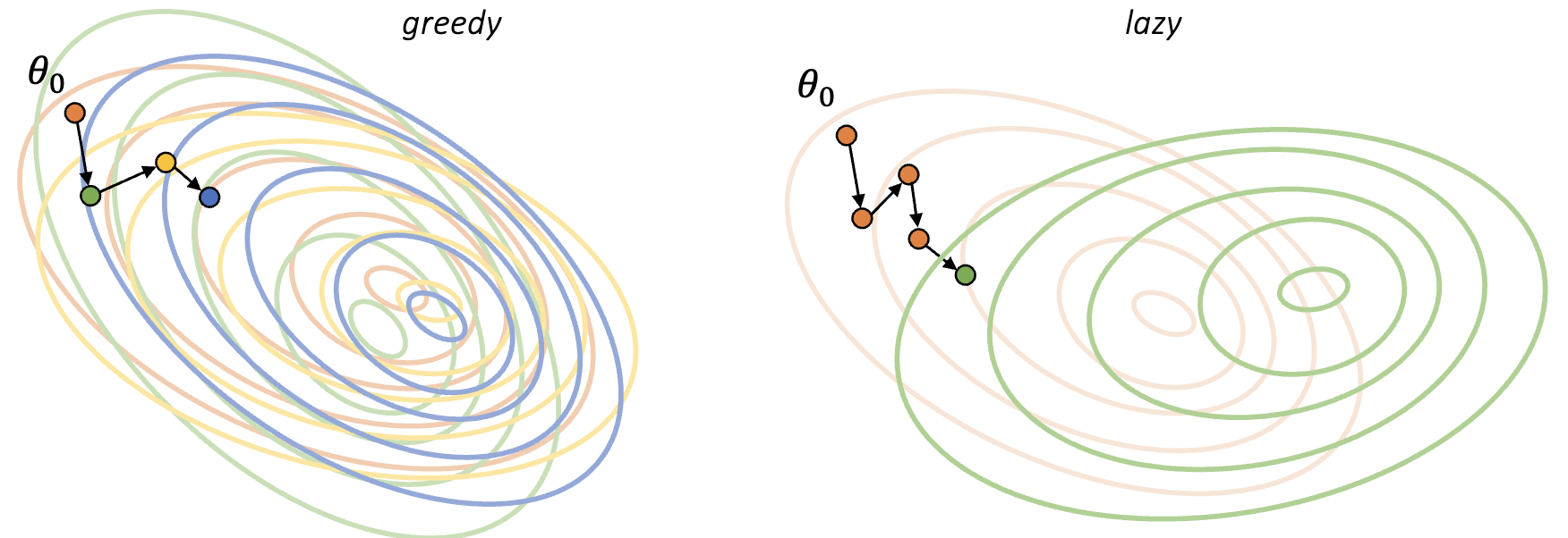
Figure 2: Greedy deploy vs. lazy deploy

To illustrate this trade-off, let us consider a natural variant of SGD that performs $n(k)$ stochastic update steps in between deployment $k$ and $k+1$ based on repeated sampling from $\mathcal{D}(\theta_{k})$. We call such a strategy lazy deploy. Mendler-Dünner et al. (2020) studied the convergence properties of lazy deploy for the case where

$$n(k)\propto k^{\alpha}$$

for $\alpha>0$. In their algorithm, the optimization problem in each step $k\geq 1$ is treated as an independent, static optimization problem and SGD with a decaying stepsize schedule is used to solve it. Thus, conceptually, the lazy deploy algorithm can be viewed as an approximation to the RRM procedure, where the approximation error decreases as $k$ grows.

Bounding the approximation error and analyzing the corresponding effect on the distribution shift, Mendler-Dünner et al. (2020) gave a convergence guarantee for lazy deploy under the same conditions as greedy deploy in Theorem 3. Their result shows that lazy deploy can reduce the number of deployments at a cost of increased sample complexity. More formally, to achieve a suboptimality $\mathrm{E}[\|\theta_{k}-{\theta_{\mathrm{PS}}}\|^{2}]\leq\delta$ the number of deployments scale as

$$\mathrm{greedy:}\;O\big{(}1/\delta\big{)}\rightarrow\mathrm{lazy}:\;O\big{(}1/\delta^{\alpha}\big{)}$$

and the corresponding sample complexity scales as

$$\mathrm{greedy:}\;O\big{(}1/\delta\big{)}\rightarrow\mathrm{lazy}:\;O\big{(}1/\delta^{\frac{1+\alpha}{\alpha}}\big{)}\,.$$

Comparing the asymptotic properties of greedy and lazy deploy illustrates that depending on the cost of sample collection and the cost of model deployment, either of the two strategies can be more desirable. Mendler-Dünner et al. (2020) further found that greedy deploy is particularly effective for weak performative shifts as it behaves like SGD in the static setting, whereas lazy deploy converges faster for larger $\epsilon$ by closely mimicking the behavior of RRM.

Beyond reducing for overheads of model deployments when searching for performatively stable points, approaches to efficiently adjust complex models to the gradually shifting distribution could be interesting to explore in the context of performative prediction. These include practical approaches to transfer learning and domain adaptation in deep learning (Long et al., 2015; Howard and Ruder, 2018) as well as recently popularized parameter-efficient fine-tuning techniques (Houlsby et al., 2019).

5 Optimizing the performative risk

Performatively stable points are not necessarily performatively optimal. Thus, finding optimal points requires different algorithmic approaches since the learner needs to take consequences of performative distribution shifts into account, rather than solely reacting to them. The main challenge of accounting for performative shifts is that the distribution map is typically not known ahead of time and $\mathcal{D}(\theta)$ can only be observed after the model $\theta$ is deployed. Thus, there is inherent uncertainty about the induced distribution of future models. In this section we discuss algorithmic approaches for finding performative optima that deal with this uncertainty by relying on sensitivity as a regularity condition on the distribution shift, without assuming any problem-specific structure of $\mathcal{D}(\theta)$.

5.1 Derivative-free optimization

A natural approach for optimizing the performative risk is to apply gradient-based optimization to the performative risk directly. As the gradient $\nabla\mathrm{PR}(\theta)$ is infeasible to compute without knowledge of the distribution map, a natural starting point is to resort to derivative-free methods. Such methods explore modifications of the current iterate to investigate how they impact the performative risk. Such zero-order local information can be used to determine directions of improvement from finite differences, to then optimize the performative risk directly. Variations of this approach were explored by Izzo et al. (2021); Miller et al. (2021); Izzo et al. (2022) and Ray et al. (2022).

However, a strong requirement for these approaches to efficiently minimize the performative risk from local information is that $\mathrm{PR}(\theta)$ satisfy convexity. Miller et al. (2021) provided sufficient conditions on the structure of the distribution map for which (strong) convexity of the static problem is preserved under performativity. In particular, they showed that if the loss is $\gamma$-strongly convex and the distribution satisfies the following stochastic dominance condition

$$\mathop{\operatorname*{\mathbb{E}}}_{z\sim\mathcal{D}(\alpha\theta_{1}+(1-\alpha)\theta_{2})}\ell(\theta;z)\leq\mathop{\operatorname*{\mathbb{E}}}_{z\sim\alpha\mathcal{D}(\theta_{1})+(1-\alpha)\mathcal{D}(\theta_{2})}\ell(\theta;z),$$

for any $\theta,\theta_{1},\theta_{2}\in\Theta$ and $\alpha\in(0,1)$, then $\mathrm{PR}(\theta)$ is $\gamma^{\prime}=\beta-2\epsilon\gamma$ strongly convex. The condition corresponds to convexity of the risk in the distribution argument. Similar conditions have been extensively studied within the literature on stochastic orders, see Shaked and Shanthikumar (2007). A stronger result holds for certain families of distributions, such as location-scale families.

In general, however, the performative risk might not satisfy any structural properties which would imply that its stationary points have low performative risk. In fact, the performative risk can be non-convex, even for convex losses and simple distribution shifts, as noted in Perdomo et al. (2020). Relying on zero-order gradient methods might help achieve local improvements, but it can lead to suboptimal solutions in many natural cases.

5.2 Bandit optimization

When $\mathrm{PR}(\theta)$ is non-convex, global exploration is necessary for finding performative optima. To this end, Jagadeesan et al. (2022) explored how tools from multi-armed bandits can be applied to guide exploration in performative prediction and find models of low performative risk.

To set up the objective formally, assume at every step a model $\theta_{t}$ is deployed, and after deployment the distribution $\mathcal{D}(\theta_{t})$ can be observed. Given the online nature of this task, we measure the quality of a sequence $\theta_{0},\theta_{1},...,\theta_{T}$ by evaluating the performative regret

$$\mathrm{Reg}(T):=\sum_{t\leq T}\mathrm{PR}(\theta_{t})-\mathrm{PR}({\theta_{\mathrm{PO}}}).$$

A key characteristic of the performative prediction problem is that after each model deployment we get to observe the induced distribution $\mathcal{D}(\theta_{t})$, rather than only bandit feedback about the reward $\mathrm{PR}(\theta_{t})$. Together with knowledge of the loss function and the structure of the reward function this additional information allows for a tighter construction of confidence bounds to guide exploration more effectively. In the following we provide the main intuition for why this leads to an algorithm with a regret bound that primarily scales with the complexity of the distribution shift, rather than the complexity of the reward function.

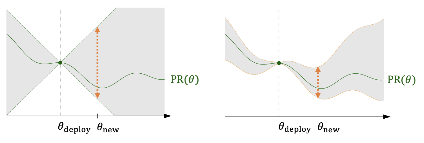
Figure 3: Confidence bounds on the performative risk. Left: using bandit feedback and Lipschitzness of the performative risk. Right: using performative feedback together with sensitivity of the distribution map and Lipschitzness of $\ell$ in $z$.

Performative confidence bounds.

Access to the distribution $\mathcal{D}(\theta_{t})$ allows the learner to infer bandit feedback about the reward $\mathrm{PR}(\theta_{t})$ but also to evaluate the $\mathrm{Risk}(\theta^{\prime};\mathcal{D}(\theta_{t}))$ for any $\theta^{\prime}\in\Theta$. Hence, for constructing confidence bounds on $\mathrm{PR}(\theta^{\prime})$ we can extrapolate from $\mathrm{Risk}(\theta^{\prime};\mathcal{D}(\theta_{t}))$, rather than extrapolating from $\mathrm{PR}(\theta_{t})$. This means it remains to deal with uncertainty due to distribution shift alone, rather than the uncertainty in the reward function. Assuming $L_{z}$-Lipschitzness of the loss in $z$ and $\epsilon$-sensitivity of the distribution map we get the following upper-confidence bound on an unexplored model $\theta^{\prime}\in\Theta$

$$\mathrm{PR}(\theta^{\prime}) \leq\min_{t}\;\mathrm{Risk}(\theta^{\prime};\mathcal{D}(\theta_{t}))+L_{z}\epsilon\|\theta^{\prime}-\theta_{t}\|\,.$$ (12)

The bound follows from the Kantorovich-Rubinstein duality applied to the Lipschitz loss function and then invoking the definition of sensitivity. We refer to Fig. 3 for contrasting the performative confidence bounds with those of classical applications of Lipschitz bandits that follow from extrapolating $\mathrm{PR}(\theta)$ under a Lipschitzness assumption of the reward function.

From the figure it can been seen that performative confidence bounds potentially allow the learner to discard high risk regions of the parameter space without ever exploring them. Furthermore, from the bound in (12) we see that the size of the confidence sets is independent of the dependence of the loss function on $\theta.$ This stands in contrast with a naive application of black box optimization techniques to $\mathrm{PR}(\theta)$. Furthermore, the extrapolation uncertainty diminishes as $\epsilon\rightarrow 0$, recovering a static problem.

Regret bound.

Building on the above construction, taking into account finite sample uncertainty and applying techniques from successive elimination to determine which model to deploy next, Jagadeesan et al. (2022) proposed an algorithm that achieves a regret of the form

$$\mathrm{Reg}(T)=\tilde{O}\left(\sqrt{T}+T^{\frac{d+1}{d+2}}(L_{z}\epsilon)^{\frac{d}{d+2}}\right)$$

where $d$ denotes the zooming dimension of the problem; an instance-dependent notion of dimensionality introduced by Kleinberg et al. (2008) that can be upper-bounded by the dimension of the parameter space for the purpose of this exposition.

Notably, a sensitivity assumption on the distribution shift is sufficient to efficiently find models of small performative risk. The regret bound scales as $\tilde{O}(\sqrt{T})$ in the case of $\epsilon=0$, since only finite sample uncertainty remains. In contrast, the regret of classical applications of Lipschitz bandits that only rely on bandit feedback about the reward would remain exponential in the problem dimension, see e.g., (Kleinberg et al., 2008). This is because in the case of no performativity the Lipschitz constant of the performative risk reduces to the Lipschitz constant of the loss function which is non-zero in general.

The asymmetric dependence of the performative risk on the model parameters together with the rich feedback model exhibits an interesting structure for the application of tools from bandit optimization to efficiently find models of small performative risk. Incorporating additional insights from the literature on multi-armed bandits in performative prediction, such as techniques for constraint and exploration as in Wu et al. (2016); Turchetta et al. (2019), could be an interesting direction for future work. See also García and Fernández (2015) for a starting point on related work in safe reinforcement learning.

6 Model-based approaches to anticipate performativity

So far the only assumption we posed on the distribution map was a mild regularity condition. However, it can be appealing to build a more precise understanding of the distribution shift and learn or posit a model for the distribution map. Such a model of $\mathcal{D}(\theta)$ can then be use to evaluate outcomes across different candidate models $\theta\in\Theta$, assess their performative risk, and compare them alongside different evaluation criteria and loss functions, without the need to further interact with the environment.

In this section we discuss several models for the distribution map from the literature that all postulate a different mechanism by which performativity occurs.

6.1 Outcome performativity

A natural mechanism by which performativity occurs is that predictions directly impact the outcome they aim to forecast. Among others, this has been documented in housing price prediction, education, as well as medical applications where predictions inform treatment decisions. This scenario is described as a special case of performative prediction. Namely, performative effects are mediated by the prediction $\hat{Y}$ and they impact the outcome variable $Y$, while features $X$ are unaffected by prediction. This assumption can be formalized in the following causal diagram for the data generating process:

Let $X=\xi_{X}$ with $\xi_{X}\sim\mathcal{D}_{x}$ denoting the feature vector that is drawn iid. from a static feature distribution. The prediction is determined as $\hat{Y}=f_{\theta}(X)$ and the outcome is determined from $X$ and $\hat{Y}$ as $Y=g(X,\hat{Y},\xi_{Y})$ where $\xi_{Y}$ denotes an exogenous noise variable. In this model the function $g$ in the structural equation for $Y$ encodes the mechanism of performativity.

Mendler-Dünner et al. (2022) were the first to study this model in the context of performative prediction. They used that the prediction $\hat{Y}$ offers a sufficient statistic for the performative distribution shift and proposed an approach they call predicting from predictions to predict $Y$ under outcome performativity. More precisely, they suggest to treat the prediction as an additional input feature when learning a model for the outcome. Thereby they lift the dynamic problem of performative prediction to a supervised learning problem of predicting $Y$ from $(X,\hat{Y})$. They provide conditions on the training data under which such a supervised learning approach can recover the true underlying causal mechanism $g$. In particular, if the training data was collected under the deployment of a prediction function $f_{\mathrm{collect}}$, predicting from predictions can recover $g$ if $f_{\mathrm{collect}}$ was appropriately randomized, it had discrete outputs, or its functional complexity was sufficiently high relative to the true underlying concept. However, if $f_{\mathrm{collect}}$ is a continuous and deterministic prediction function, this is not the case in general. The reason is that the induced training data does not permit causal identifiability.

Perdomo et al. (2023) used a test for performativity from Mendler-Dünner et al. (2022) in a major evaluation of a early warning system for high school dropout used across the state of Wisconsin. If the early warning system were effective, predictions of dropout risk should be predictive of the actual outcome and have an effect that is self-negating.

Kim and Perdomo (2023) studied the task of learning the conditional distribution $P(Y|X,\hat{Y})$ underlying the distribution map through the lens of outcome indistinguishability (Dwork et al., 2021). They call a model for the conditional distribution a performative omnipredictor with respect to a class of loss functions $\mathcal{L}$ and a hypothesis class $\mathcal{F}$ if it allows us to identify the performative optimal model within a model family $\mathcal{F}$ for any $\ell\in\mathcal{L}$. The optimality concept of an omnipredictor is adapted from the supervised learning setting where it was introduced by Gopalan et al. (2021). The structural equation $g$ defining the true data generating process offers such an omnipredictor. However, irrespective of the complexity of $g$, Kim and Perdomo (2023) showed that for sufficiently simple classes $\mathcal{L}$ and $\mathcal{H}$ there exists a simple omnipredictor. Similar to Mendler-Dünner et al. (2022) they suggest finding such as omnipredictor using primitives from supervised learning. Crucially, their approach requires training data collected under the deployment of a randomized predictor to guarantee identifiability; it does not apply to the typical case of a deterministic predictor $f_{\mathrm{collect}}$. This could pose an obstacle in practice when learning from observational data.

Other goals such as testing for performativity from non-experimental data are an interesting direction for future work.

6.2 Strategic classification and microfoundations

A different set of assumptions underlies the model of strategic classification (Brückner and Scheffer, 2011; Hardt et al., 2016a). In this line of work, the response to a predictor derives from standard economic assumptions of a rational, representative agent, maximizing her utility function. These assumption sometimes go by the name of microfoundations. The literature on this topic is vast and interdisciplinary, but see Janssen (2005) for a starting point. The general idea of microfoundations is to derive aggregate response functions from microeconomic principles of utility theory and rational behavior.

Concretely, in this setting individuals strategically modify their features in response to a predictor with the goal of achieving a better outcome. We assume a perfectly rational and utility maximizing agent. We further assume that all individuals strategize in the same way, which justifies considering one representative agent. The firm leads by deploying a predictor. The agent follows by changing her features with full knowledge of the deployed classifier. This sequential two player game is an instance of a Stackelberg game. The agent’s action $x(\theta)$ in response to a model $\theta$ satisfies

$$x(\theta)=\operatorname*{arg\,max}_{x^{\prime}\in\mathcal{X}}f_{\theta}(x^{\prime})-c(x_{\mathrm{orig}},x^{\prime})\,$$ (13)

where $c(x_{\mathrm{orig}},x^{\prime})$ denotes the cost of moving from the original features $x_{\mathrm{orig}}$ to the new features $x^{\prime}$. Thus, the agent engages in feature manipulation so long as the benefit of a positive prediction exceeds the cost of feature manipulation. The distribution map is then determined by aggregating the agent behavior across the population.

This model can capture different types of strategic behavior around machine learning applications. Often described as gaming the classifier, the strategic behavior can also represent attempts at self-improvement (Miller et al., 2020; Kleinberg and Raghavan, 2020).

Due to the precise characterization of the agent’s response function, the model lends itself to mathematical analysis. However, the standard microfoundations of a rational representative agent are the subject of well-known critiques in macroeconomics (Kirman, 1992; Stiglitz, 2018) and sociology (Collins, 1981). Jagadeesan et al. (2021) pointed out important drawbacks in the context of prediction. In particular, standard microfoundations lead to the following problems:

• There are sharp discontinuities in the response to a decision rule that are often not descriptive of the empirical reality.

• If only a positive fraction of agents act non strategically stable points cease to exist.

• Performatively optimal decision rules maximize a measure of negative externality known as social burden (Milli et al., 2019) within a broad class of assumptions about agent behavior.

6.3 Parametric models

Miller et al. (2021) study distribution maps $\mathcal{D}(\theta)$ that can be parameterized by a location-scale family. That is, performative effects are such that samples $z\sim\mathcal{D}(\theta)$ can be expressed as $z=z_{0}+\mu\theta$ where $z_{0}\sim\mathcal{D}_{0}$ is a sub-Gaussian random variable, independent of $\theta$, and $\mu$ denotes the location map. Such a parametric model is particularly appealing as it leads to desirable convexity properties of the performative risk. Izzo et al. (2021) use an exponential family to model the distribution map, motivated by the approximation power of Gaussian mixtures. Concretely, they model the distribution map as a mixture of $K$ normal distributions with means that depends on the deployed model and fixed covariances, such that $\mathcal{D}(\theta)=\sum_{i=1}^{k}\alpha_{i}\mathcal{N}(\mu_{i}(\theta),\Sigma_{i})$ with positive coefficients $\alpha_{i}>0$ summing to one.

Model misspecification.

Lin and Zrnic (2023) characterized regimes where model-based approaches, even if misspecified, can be beneficial for learning under performativity. In particular, they show that in the regime of finite samples, model-based approaches can find near performative optimal points more efficiently compared to structure-agnostic approaches such as discussed in Section 5. To provide intuition for this claim, let $\mathcal{D}_{\beta}(\theta)$ be a parameterized model for the distribution map $\mathcal{D}(\theta)$, and denote $\hat{\theta}_{\mathrm{PO},\beta}$ the performative optima computed under this model. Let $\hat{\beta}$ be a finite sample estimate of $\beta$. Then the excess risk of a model based approach decomposes into a model misspecification term and a statistical error term, and it is bounded by

$$\mathrm{PR}(\hat{\theta}_{\mathrm{PO},{\hat{\beta}}})-\mathrm{PR}({\theta_{\mathrm{PO}}})\leq\mathrm{MisspecErr}+\tilde{O}\Big{(}\frac{1}{\sqrt{n}}\Big{)}$$

While the misspecification error is irreducible, the statistical error vanishes at a rate $\tilde{O}(n^{-\frac{1}{2}})$. In contrast, the bandit algorithm discussed in Section 5.2 does not suffer from model misspecification error, but has an exceedingly slow statistical rate of $\tilde{O}(n^{\frac{1}{1+d}})$. Thus, if the misspecification error is not too large, and $n$ is sufficiently small, model-based approaches can outperform model-free methods.

6.4 Algorithmic fairness and interventions

The specifics of how predictions affect a population is a concern central to the active research area of fairness in machine learning, see Barocas et al. (2023). Researchers in this area have proposed numerous fairness criteria that formalize different notions of equality between different groups in the population, defined along the lines of categories such as race or gender. One criterion, for example, asks to equalize the true positive rate of the predictor in different demographic groups (Cole, 1973; Hardt et al., 2016b).

Such fairness criteria are typically thought of as constraints on a static supervised learning objective. In a departure from this perspective, Liu et al. (2018) proposed a notion of delayed impact that models how decisions affect a population in the long run. As an example, think of how lending practices based on a credit score affect welfare in the population. A default on a loan not only diminishes profit for the lender, it also impoverishes the individual who defaulted. The latter effect is typically not modeled in supervised learning. The results show that standard fairness criteria, when enforced as constraints on optimization, may not have a positive long-term impact on a disadvantaged group, relative to unconstrained optimization.

Delayed impact is an instance of performative prediction. It illustrates the importance of performativity as a criterion in the evaluation of machine learning. Adding further support to this point, Fuster et al. (2022) showed how to introduction of machine learning in lending can have a disparate effect on borrowers of different racial groups. In a similar vein, Hu and Chen (2018) studied the same problem in labor markets. Ensign et al. (2018) studied feedback loops in predictive policing. Taori and Hashimoto (2023) showed how performativity can amplify dataset biases. The celebrated work of Coate and Loury (1993) is an important intellectual precursor of the development of dynamic models in algorithmic fairness.

7 The role of power in prediction

Morgenstern already knew that performativity was a consequence of authority and reach. He recognized that the strength of performativity varied from the case of a monopoly forecast to the case of multiple competing forecasts (Morgenstern, 1928, p.111). Put differently, the extent to which predictions can influence the course of events depends on the power of those who make the prediction. The traffic predictions of a service used by millions of drivers has the ability to significantly shape traffic. Were a competing service to enter the market, its predictions would affect a smaller user base and hence show a lesser effect on traffic patterns.

If power is the cause of performativity, we can ask if it is possible to measure power through the strength of performativity. This idea is the starting point for the definition of performative power by Hardt et al. (2022) that we turn to next.

Our running example is a digital platform that can influence participants on its platform through a set of actions. To make this concrete, think of how a search engine provider can influence what users click on through how content is presented. For instance, ads may be displayed before or after the first organic search results. We’re generally interested in how much a platform can influence participants through its algorithmic actions. Such questions are at the heart of ongoing antitrust investigations into digital platforms (Crémer et al., 2019; Stigler Committee, 2019).

7.1 Performative power

Fix a set $\mathcal{U}$ of participants interacting with a firm under investigation. Each unit $u\in\mathcal{U}$ is associated with a data point $z(u)$. Fix a metric $\mathrm{dist}(z,z^{\prime})$ over the space of data points. Let $\mathcal{F}$ denote the set of actions a firm can take. We typically think of an action $f\in\mathcal{F}$ as the deployment of a specific algorithmic change at a fixed point in time. For each participant $u\in\mathcal{U}$ and action $f\in\mathcal{F}$, we denote by $z_{f}(u)$ the potential outcome random variable representing the counterfactual data of participant $u$ if the firm were to take action $f$.

Definition 4 (Performative Power).

Given a population $\mathcal{U}$, an action set $\mathcal{F}$, potential outcome pairs $(z(u),z_{f}(u))$ for each unit $u\in\mathcal{U}$ and action $f\in\mathcal{F}$, and a metric $\mathrm{dist}$ over the space of data points, we define the performative power of the firm as

$$\mathrm{P}:=\sup_{f\in\mathcal{F}}\;\frac{1}{|\mathcal{U}|}\sum_{u\in\mathcal{U}}\operatorname*{\mathbb{E}}\left[\mathrm{dist}\left(z(u),z_{f}(u)\right)\right]\,,$$

where the expectation is over the randomness in the potential outcomes.

The definition takes a supremum over possible actions a firm can take at a specific point in time. We can therefore lower bound performative power by estimating the causal effect of any given action $f\in\mathcal{F}.$ Put differently, performative power speaks to the potential for influence, not necessarily realized influence.

Performative power is a statistical causal notion. As such it does not require specification of the market in which the firm operates. Digital platforms typically operate in two-sided markets mediating between content creators or service providers and consumers. The definition applies to both sides of the market. We could study how much a change in a ranking algorithm influences the wellbeing of video producers. Or we could study how much the positioning of search results steers visitors toward certain product offerings.

Before we turn to the question of empirical estimation, we collect some useful theoretical properties that the definition enjoys.

7.2 Theoretical properties

Hardt et al. (2022) investigated the theoretical properties of performative power in a simple microfoundations model similar to the one we saw in Section 6.2. They found:

1. A monopoly firm maximizes performative power. Participants are willing to incur a cost equal to utility for the service.

2. A firm’s ability to personalize predictions increases performative power.

3. Outside options decrease performative power.

4. When multiple platforms compete over users with services that are perfect substitutes, then already two firms lead to zero performative power. This result is analogous to the Bertrand competition where two competing firms setting prices for identical goods simultaneously are sufficient for zero profit, i.e., competitive prices. (Bertrand, 1883).

These propositions suggest that the definition is sensitive to some key concepts from the study of competition. The mode of investigation here is to see how the definition squares against familiar economic concepts. An interesting avenue for future work is to deepen the study of performative power in the context of established economic models. For example, it may be insightful to understand how performative power behaves under market entry, mergers and acquisitions, and common ownership. However, a key desideratum for the definition of performative power is to illuminate settings where traditional concepts of market power are difficult to apply. There is extensive discussion about the difficulty of applying classical tools to digital economies (Crémer et al., 2019; Stigler Committee, 2019). The goal is not to replace existing tools where they work fine. Rather performative power is a new notion of power tailored to the challenging case of digital platforms, where existing tools may be insufficient.

Steering.

Performative power is closely related to the notion of steering that we can formalize in the language of performative prediction. To do so, it is helpful to decompose performative risk into two terms. Observe that the model $\theta$ shows up in two places in the definition of performative risk: in the distribution $\mathcal{D}({\theta})$ and in the loss $\ell(\theta;\,z)$. Thus, for any choice of model $\phi$, we can decompose the performative risk $\mathrm{PR}(\theta)$ as:

$$\mathrm{PR}(\theta) =\mathrm{Risk}(\theta,\mathcal{D}(\phi))+\left(\mathrm{Risk}(\theta,\mathcal{D}(\theta))-\mathrm{Risk}(\theta,\mathcal{D}(\phi))\right)$$ (14)

Read this tautology as follows. Suppose we’re currently in a baseline state $\mathcal{D}(\phi)$ given by a currently deployed model $\phi$. Consider moving to a new model $\theta$. The performative risk of $\theta$ depends on two terms. The first expresses how well the model fares in current conditions. It’s just the conventional risk from supervised learning under the baseline distribution. The second term quantifies how much we stand to gain by changing the data-generating distribution to the new state $\mathcal{D}(\theta)$. In other words, there are two ways to be good at performative prediction. One is to optimize well in current conditions. The other is to steer to a new distribution that suits us better. The first mechanism is well known. It’s what we conventionally call learning. The second mechanism of prediction is new and specific to performative prediction. It’s what we call steering.

Performative power bounds the extent to which a firm can, in principle, utilize the mechanism of steering to its own advantage. A firm with zero performative power is confined to optimizing its objective against current conditions. A firm with positive performative power can stand to gain from changing conditions. This dichotomy is analogous to the distinction between a price taker and a price maker in economics.

7.3 Performative power via causal inference

Performative power is a causal notion. Having specified the sets $\mathcal{F}$ and $\mathcal{U}$, estimating performative power amounts to causal inference involving the potential outcome variables $z_{f}(u)$ for unit $u\in\mathcal{U}$ and action $f\in\mathcal{F}$. In an experimental design, the investigator deploys a suitably chosen action to estimate the effect. In an observational design, an investigator is able to identify performative power without an experimental intervention on the platform. Neither route requires understanding the specifics of the market in which the firm operates. It is not even necessary to know the firm’s objective function, how it optimizes its objective, and whether it successfully achieves its objective. In practice, the dynamic process that generates the potential outcome $z_{f}(u)$ may be complex, but this complexity does not enter the definition. Consequently, the definition applies to complex multisided digital economies that defy mathematical specification.

Causal effect of position.

To illustrate the definition, we work through a specific strategy to give lower bounds on performative power using causal inference about the effect of content positioning in digital services. Our running example is that of a digital platform that can choose to place content in one of several positions. Major ongoing antitrust cases allege that platforms used positioning strategically to steer users toward their own product offerings.

To quote from a major antitrust case by the European Commission against Google:

[T]he General Court [of the European Union] finds that, by favouring its own comparison shopping service on its general results pages through more favourable display and positioning, while relegating the results from competing comparison services in those pages by means of ranking algorithms, Google departed from competition on the merits.

Similarly, a recent complaint by the Federal Trade Commission against Amazon includes amongst its allegations the claim that

[…] shoppers consequently face less relevant search results and are steered toward more expensive products.

Further:

Amazon deliberately steers shoppers away from offers that are not featured in the Buy Box.

Note the invocation of the notion of steering to describe Amazon’s practices. Performative power gives a rigorous and effective set of tools to support precisely such claims.

Formal setting.

We assume that there are $c$ pieces of content $\mathcal{C}=\{0,1,2,\dots,c-1\}$ that the platform can present in $m$ display slots. We focus on the case of two display slots ($m=2$) since it already encapsulates the main idea. The first display slot is more desirable as it is more likely to catch the viewer’s attention. Researchers have investigated the causal effect of position on consumption, often via quasi-experimental methods such as regression discontinuity designs, but also through experimentation in the form of A/B tests.

Definition 5 (Causal effect of position).

Let the treatment $T\in\{0,1\}$ be the action of flipping the content in the first and second display slots for a viewer $u$, and let the potential outcome variable $Y_{t}(u)$ indicate whether, under the treatment $T=t$, viewer $u$ consumes the content that is initially in the first display slot. We call the corresponding average treatment effect

$$\beta=\Big{|}\frac{1}{|\mathcal{U}|}\sum_{u\in\mathcal{U}}\mathbb{E}\left[Y_{1}(u)-Y_{0}(u)\right]\Big{|}$$

the causal effect of position in a population of viewers $\mathcal{U}$, where the expectation is taken over the randomness in the potential outcomes.

To give an example, Narayanan and Kalyanam (2015) estimated the causal effect of position in search advertising, where advertisements are displayed across a number of ordered slots whenever a keyword is searched. They measured the causal effect of position on click-through rate of participants.

The following theorem confirms that the causal effect of position lower bounds performative power provided that units don’t interfere. In the context of search advertising, this assumption means that one user’s clicks don’t influence another user’s clicks. Since users generally do not observe each other’s clicks, it’s reasonable to assume that this assumption largely holds within a short time window in the context of search.

Theorem 6 (Hardt et al. (2022)).

Let $\mathrm{P}$ be performative power as instantiated above. Assume no interference between experimental units. Then, performative power is at least as large as the causal effect of position $\beta\leq\mathrm{P}\,.$

The proof idea is to instantiate the definition of performative power such that the action corresponds to flipping the content position from the first to the second position. However, there’s an important hurdle. To show that performative power is large, we need to apply the firm’s action simultaneously to all units in the population. If units were to interfere, then it would not be clear that the causal effect extrapolates from a single unit to the whole population. This is what the no interference assumption takes care of.

In related work, Cheng et al. (2023) proposed an observational design to estimate performative power in a dynamical systems model of digital content recommendation.

8 Algorithmic collective action

Previously we studied how much a firm can steer a population through its predictions. We now turn the question on its head and ask: How can a fraction of the population steer the predictions of a firm?

Hardt et al. (2023) studied this question from the perspective of collective action. A fraction of participants on a platform strategically modify their data so as to influence the behavior of the predictor learned by the platform. One motivation for such collective strategies is to improve the conditions of gig workers on digital platforms (Chen, 2018; Wood et al., 2019; Gray and Suri, 2019; Schor et al., 2020; Schor, 2021).

Hardt et al. (2023) proposed a simple model to study algorithmic collective action in machine learning. The size of the collective is specified by a value $\alpha>0$ that corresponds to the fraction of participating individuals in a population drawn from a base distribution $\mathcal{P}_{0}.$ The firm observes the mixture distribution

$$\mathcal{P}=\alpha\mathcal{P}^{*}+(1-\alpha)\mathcal{P}_{0}\,,$$

where $\mathcal{P}^{*}$ depends on the strategy of the collective, and runs a learning algorithm $\mathcal{A}$ on $\mathcal{P}$. We illustrate the case of an optimal firm that has full knowledge of the distribution $\mathcal{P}$. The firm chooses the Bayes optimal predictor $f=\mathcal{A}(\mathcal{P})$ on the distribution $\mathcal{P}$.

8.1 Effectiveness of signal planting strategy

In the context of classification, a natural objective for the collective is to correlate a hidden signal $g(x)$ applied to a data point $x$ with a target label $y^{*}.$ To do so, given a data point $(x,y),$ the collective applies the signal function $g(\cdot)$ to $x$ and switches the label from $y$ to $y^{*}$ at training time. That is, $\mathcal{P}^{*}$ is the distribution of $(g(x),y^{*})$ for a random draw of a labeled data point $(x,y)$ from $\mathcal{P}_{0}$. In practice, the signal $g(x)$ may correspond to adding a hidden watermark in image and video content, or subtle syntactic changes in text. It is reasonable to assume that individuals are indifferent to such inconsequential changes. Conventional wisdom in machine learning has it that such hidden signals are easy to come by in practice (Liu et al., 2017; Chen et al., 2017; Gu et al., 2019).

At test time, an individual given a data point $(x,y)$ succeeds if $f(g(x))=y^{*}$. We denote the success probability of the strategy by

$$S(\alpha)=\Pr_{x\sim\mathcal{P}_{0}}\left\{f(g(x))=y^{*}\right\}\,.$$

A theorem shows that a collective of vanishing fractional size succeeds with high probability by implementing this strategy, provided that the signal $g(x)$ is unlikely to be encountered in the base distribution $\mathcal{P}_{0}$. We denote the density of the signal set under the base distribution by $\xi=\mathcal{P}_{0}(\{g(x)\colon x\in\mathcal{X}\}).$

Theorem 7 (Hardt et al. (2023)).

Under the above assumptions, the success probability of the collective is lower bounded as:

$$S(\alpha)\geq 1-\frac{1-\alpha}{\alpha}\cdot\xi\,.$$

The theorem has various extensions. The firm need not be optimal. The collective need not be able to change labels. Up to some quantitative loss, the result still holds.

But on its own, the theorem only shows how the collective can influence predictions. It does not speak about actual outcomes, such as monetary rewards for the collective. Surely, the collective is also interested in the latter and not just the former. Performativity provides the necessary link between predictions and outcomes to talk about incentives of the collective. We present this essential idea here.

8.2 Algorithmic collective action under performativity

Consider an outcome variable

$$Y=h(X)+\beta f(X)+Z\,,$$

where $Z$ is exogenous noise (i.e., independent of $X$) of mean $0$. Think of $Y$ as the revenue earned by an offering $X$ on a platform. Here, $f(X)$ is a binary predictor based on which the platform decides whether to promote the offering $X$ in some form. The term $h(X)$ captures the baseline revenue that offering $X$ earns absent the platform intervention.

Assume the collective succeeded in finding a signal function $g$ such that the baseline revenue $h$ is invariant under application of the signal function, i.e., $h(g(x))=h(x)$ for all $x\in\mathcal{X}.$ Let $C$ indicate the event that the drawn data point belongs to an individual participating in the collective. The expected revenue is $\operatorname*{\mathbb{E}}[h(X)],$ whereas the realized revenue for the collective is $\operatorname*{\mathbb{E}}[Y\mid C]$. It is not difficult to show that

$$\operatorname*{\mathbb{E}}\left[Y\mid C\right]-\operatorname*{\mathbb{E}}\left[h(X)\right]\geq S(\alpha)\beta\,.$$ (15)

Assuming a rare enough signal with $\xi\leq\alpha/2,$ Theorem 7 shows that the revenue increase for the collective is lower bounded by $\beta/2.$ In other words, the strength of performativity determines the realized payoff for the collective. To prove Equation 15, note:

$$\operatorname*{\mathbb{E}}\left[Y\mid C\right] =\operatorname*{\mathbb{E}}\left[h(g(X))+\beta f(g(X))+Z\mid C\right]$$

$$=\operatorname*{\mathbb{E}}\left[h(g(X))\right]+\beta\operatorname*{\mathbb{E}}\left[f(g(X))\right]+\operatorname*{\mathbb{E}}\left[Z\mid C\right]$$

$$=\operatorname*{\mathbb{E}}\left[h(X)\right]+\beta\Pr\left\{f(g(X))=1\right\}$$

$$=\operatorname*{\mathbb{E}}\left[h(X)\right]+S(\alpha)\beta$$

This simple observation gives a first indication that there may be a monetary incentive to algorithmic collective action. Incentives and dynamics of collective action have been studied extensively since Olson (1965). It is an interesting direction for future work to study these problems in the context of predictive systems. Better understanding incentives in algorithmic systems may also help move beyond adversarial attack models commonly studied in the machine learning community.

9 Discussion

Performativity is a ubiquitous phenomenon in the context of prediction. We can observe it in many applications of machine learning. Predictions on digital platforms, be it for online recommendation, content moderation, or digital advertising, are one particularly rich class of examples. But the authors would go so far as to conjecture that any significant social prediction problem has some aspect of performativity. While performativity is ubiquitous, the strength of performativity has an important quantifier. It depends on the power, in terms of scale, reach, and visibility, of the predictor. This property of performativity has far-reaching consequences. If power is the cause of performativity, we can measure power through the strength of performativity. This principle forms the basis of a formal notion of power in the context of prediction.

Performativity is also a notion. We can use this notion to think about what machine learning systems do and ought to be doing. As such, the notion becomes a criterion in the design and evaluation of machine learning systems in social contexts. In the same way that we think about machine learning systems in terms of other criteria, such as accuracy or computational efficiency, we propose adding performativity to the principal axes along which we scrutinize predictive systems. When predictions have consequences, the predictor becomes a point of intervention. This cuts two ways. An institution can use predictions toward social and economic objectives they seek. Individuals can leverage their data to influence social outcomes through the predictor trained on the data.

Performative prediction is a framework to study performativity as a phenomenon and to formalize the notion within the context of supervised learning. The framework establishes the necessary formal language and definitions for its dual use in the study of performativity as a phenomenon and a criterion. Compared with traditional supervised learning, there are two ways to be good at performative prediction. One is the familiar mechanism to learn patterns on current data. The other is to steer the data-generating process in a different direction. To appreciate this distinction, recall the tautology we encountered earlier. Suppose we’re in a state of the world resulting from deploying the model $\theta_{0}$ and we consider moving to a new model $\theta$. We can express its performative risk as

$$\mathrm{PR}(\theta)=\mathrm{Risk}(\theta,\mathcal{D}(\theta_{0}))+\big{(}\mathrm{Risk}(\theta,\mathcal{D}(\theta))-\mathrm{Risk}(\theta,\mathcal{D}(\theta_{0}))\big{)}\,.$$

The first term on the right hand side captures how well we optimize in current conditions. The second captures how much we stand to gain from steering the data toward a new distribution.

Our conception of performative prediction excludes some important interdisciplinary perspectives. The celebrated work of Mackenzie (MacKenzie et al., 2007; MacKenzie, 2008), for example, speaks to the performativity of economic theory. Here it is the practice of applying economic theory in financial markets and not the model’s predictions per se that are performative. Another notable form of performativity that is not captured by our framework is Hacking’s looping effect. Hacking (1995) describes how classification creates and changes social categories in an ongoing loop. This effect arises in machine learning applications as well, but is not adequately captured in our formalism. There is a vast literature on performativity in philosophy and sociology starting with the works of Austin (1975), Merton (1948), and Buck (1963) who called the problem reflexive prediction, that we cannot survey here. See Mackinnon (2005); Mäki (2013); Khosrowi (2023) for additional pointers and discussion.

Although the definition of performative prediction is recent, work in this area already spans a remarkable scope. Questions of strategic behavior, algorithmic fairness, prediction as intervention, power in digital economies, and collective action in algorithmic systems, to name a few, all benefit from the perspective of performative prediction. The problems that arise are technically rich and thrive on beautiful connections with optimization, statistics, economics, causal inference, and control theory. We hope that this survey provided a helpful introduction that has enticed the reader to this emerging area.

References

- Austin (1975) John Langshaw Austin. How to do things with words, volume 88. Oxford university press, 1975.
- Barocas et al. (2023) Solon Barocas, Moritz Hardt, and Arvind Narayanan. Fairness and Machine Learning: Limitations and Opportunities. MIT Press, 2023.
- Bertrand (1883) Joseph Bertrand. Théorie mathématique de la richesse sociale. Journal des savants, 67(1883):499–508, 1883.
- Bottou et al. (2018) Léon Bottou, Frank E. Curtis, and Jorge Nocedal. Optimization methods for large-scale machine learning. SIAM Review, 60(2):223–311, 2018.
- Brown et al. (2022) Gavin Brown, Shlomi Hod, and Iden Kalemaj. Performative prediction in a stateful world. In International Conference on Artificial Intelligence and Statistics (AISTATS), volume 151, pages 6045–6061. PMLR, 2022.
- Brückner and Scheffer (2011) Michael Brückner and Tobias Scheffer. Stackelberg games for adversarial prediction problems. In ACM SIGKDD, pages 547–555, 2011.
- Buck (1963) Roger C Buck. Reflexive predictions. Philosophy of Science, 30(4):359–369, 1963.
- Chen (2018) Julie Yujie Chen. Thrown under the bus and outrunning it! The logic of Didi and taxi drivers’ labour and activism in the on-demand economy. New Media & Society, 20(8):2691–2711, 2018.
- Chen et al. (2017) Xinyun Chen, Chang Liu, Bo Li, Kimberly Lu, and Dawn Song. Targeted backdoor attacks on deep learning systems using data poisoning. ArXiv preprint arXiv:1712.05526, 2017.
- Cheng et al. (2023) Gary Cheng, Moritz Hardt, and Celestine Mendler-Dünner. Causal inference out of control: Estimating the steerability of consumption. arXiv preprint arXiv:2302.04989, 2023.
- Coate and Loury (1993) Stephen Coate and Glenn C Loury. Will affirmative-action policies eliminate negative stereotypes? The American Economic Review, pages 1220–1240, 1993.
- Cole (1973) Nancy S Cole. Bias in selection. Journal of educational measurement, 10(4):237–255, 1973.
- Collins (1981) Randall Collins. On the microfoundations of macrosociology. American journal of sociology, 86(5):984–1014, 1981.
- Crémer et al. (2019) Jacques Crémer, Yves-Alexandre de Montjoye, and Heike Schweitzer. Competition Policy for the digital era : Final report. Publications Office of the European Union, 2019.
- Drusvyatskiy and Xiao (2023) Dmitriy Drusvyatskiy and Lin Xiao. Stochastic optimization with decision-dependent distributions. Mathematics of Operations Research, 48(2):954–998, 2023.
- Dwork et al. (2021) Cynthia Dwork, Michael P. Kim, Omer Reingold, Guy N. Rothblum, and Gal Yona. Outcome indistinguishability. In Symposium on Theory of Computing (STOC), page 1095–1108, 2021.
- Ensign et al. (2018) Danielle Ensign, Sorelle A Friedler, Scott Neville, Carlos Scheidegger, and Suresh Venkatasubramanian. Runaway feedback loops in predictive policing. In Conference on fairness, accountability and transparency, pages 160–171. PMLR, 2018.
- Fuster et al. (2022) Andreas Fuster, Paul Goldsmith-Pinkham, Tarun Ramadorai, and Ansgar Walther. Predictably unequal? the effects of machine learning on credit markets. The Journal of Finance, 77(1):5–47, 2022.
- García and Fernández (2015) Javier García and Fernando Fernández. A comprehensive survey on safe reinforcement learning. JMLR, 16(1):1437–1480, 2015.
- Gopalan et al. (2021) Parikshit Gopalan, Adam Tauman Kalai, Omer Reingold, Vatsal Sharan, and Udi Wieder. Omnipredictors. In Innovations in Theoretical Computer Science Conference (ITCS), 2021.
- Gray and Suri (2019) Mary L Gray and Siddharth Suri. Ghost work: How to stop Silicon Valley from building a new global underclass. Eamon Dolan Books, 2019.