AirFL-Mem: Improving Communication-Learning Trade-Off by Long-Term Memory

Abstract

Addressing the communication bottleneck inherent in federated learning (FL), over-the-air FL (AirFL) has emerged as a promising solution, which is, however, hampered by deep fading conditions. In this paper, we propose AirFL-Mem, a novel scheme designed to mitigate the impact of deep fading by implementing a long-term memory mechanism. Convergence bounds are provided that account for long-term memory, as well as for existing AirFL variants with short-term memory, for general non-convex objectives. The theory demonstrates that AirFL-Mem exhibits the same convergence rate of federated averaging (FedAvg) with ideal communication, while the performance of existing schemes is generally limited by error floors. The theoretical results are also leveraged to propose a novel convex optimization strategy for the truncation threshold used for power control in the presence of Rayleigh fading channels. Experimental results validate the analysis, confirming the advantages of a long-term memory mechanism for the mitigation of deep fading.

I Introduction

Over-the-air FL (AirFL) has emerged from information-theoretic studies [1] as a promising approach to enable model aggregation in wireless implementations of federated learning (FL) [2]. A well-known problem with AirFL is that devices experience different fading conditions, causing the aggregated model estimated by the central server to deviate from the desired model average, unless strict power constraints mechanisms are applied.

In the presence of channel state information at the transmitter (CSIT), the typical solution to this problem is to ensure signal alignment through truncated channel inversion [2, 3, 4, 5, 6, 7]. Truncation entails that only a subset of model parameters reach the server, causing the erasure of potentially important information. Reference [7] proposed to mitigate the resulting channel-driven sparsification of model information via error feedback. Specifically, the approach therein applies a short-term memory mechanism that operates across two successive iterations. However, no theoretical guarantees are currently available for this mitigation strategy. This paper aims at addressing this knowledge gap, revealing through theoretical bounds that error feedback based on longer-term memory mechanisms is generally necessary to combat the effect of deep fading on truncated channel inversion.

To provide additional context for this work, other solutions to the problem of deep fading in AirFL in the presence of CSIT include phase-only compensation [8, 9], transmission weight optimization [10], and device selection [11]. Without CSIT, references [12, 13, 14, 15] studied the convergence of AirFL over broadband channels, and improved the performance by exploiting the channel hardening property of massive multiple-input and multiple-output (MIMO) channels. Error-feedback-based transmission has been widely adopted for communication-efficient FL with the aim of compensating losses for model-update information. Such methods compensate for accumulated errors due to artificially induced sparsity or quantization in the next-round transmission [7, 16, 17, 18, 19]. For digital transmission-based FL, the authors of [19] applied a memory vector in digital FL schemes to compensate for both compression and reconstruction errors.

Overall, in this paper, inspired by sparsified stochastic gradient descent (SGD) with memory [16], we introduce AirFL-Mem, an AirFL protocol that implements a long-term memory mechanism for error feedback in truncated channel inversion. Furthermore, we analyze the role of memory in error feedback via convergence bounds. Our contributions are as follows:

• We provide convergence bounds for AirFL-Mem, as well as for the existing variant with short-term memory [7], demonstrating that AirFL-Mem achieves the same convergence rate as FedAvg in perfect communication conditions [20], while a shorter memory may cause an error floor.

• Based on the derived bounds, we introduce a novel convex optimization-based truncation-threshold selection scheme for the implementation of AirFL-Mem.

The rest of the paper is organized as follows. Sec. II introduces system level and preliminaries. Sec. III describes AirFL-Mem, while Sec. IV describes the derived theoretical bounds. Sec. V presents the proposed optimization scheme for the power control thresholds, and Sec. VI covers numerical results, with Sec. VII completing the paper.

II System Model and Preliminaries

In this section, we consider an AirFL system in which a set $[K]\triangleq\{1,\ldots,K\}$ of devices transmit their machine learning models to an edge server over a Gaussian multiple access channel (MAC) fading channel. In this section, we first introduce the vanilla FL protocol premised on ideal and noiseless communications, and then describe the considered communication model accounting for fading and noise.

II-A Learning Protocol (Vanilla FL)

In the FL setup, each device $k\in[K]$, possesses a distinct local dataset denoted as $\mathcal{D}_{k}$. All devices share a machine learning model, e.g., a neural network or a transformer parameterized by a vector $\mbox{\boldmath{$\theta$}}\in\mathbb{R}^{d\times 1}$. The objective of the FL system is to collaboratively solve the empirical loss minimization problem

$$\mathrm{(P0)}: ~{}\mathop{\mathtt{Minimize}}_{\mbox{\boldmath{$\theta$}}}~{}~{}~{}f(\mbox{\boldmath{$\theta$}})\triangleq\frac{1}{K}\sum_{k=1}^{K}f_{k}(\mbox{\boldmath{$\theta$}}),$$

where $f(\mbox{\boldmath{$\theta$}})$ represents the global empirical loss function; and $f_{k}(\mbox{\boldmath{$\theta$}})=1/|\mathcal{D}_{k}|\sum_{\bm{\xi}\in\mathcal{D}_{k}}\mathcal{L}(\mbox{\boldmath{$\theta$}};\bm{\xi})$ represents the local empirical loss function for device $k\in[K]$. The cardinality operation $|\cdot|$ denotes the size of a given set, and the notation $\mathcal{L}(\mbox{\boldmath{$\theta$}};\bm{\xi})$ indicates the loss function evaluated at parameter $\theta$ with respect to (w.r.t) the data sample $\bm{\xi}$.

In the following, we briefly review the standard FedAvg protocol [20]. Let $t\in\{0,\ldots,T-1\}$ denote the index of global communication rounds or, equivalently, of global iterations. At the $t$-th global iteration, individual devices obtain a localized parameter $\mbox{\boldmath{$\theta$}}_{k}^{(t)}$ that approximates the solution $\mbox{\boldmath{$\theta$}}^{(t)}$ to problem ($\mathtt{P0}$) by minimizing the local loss $f_{k}(\mbox{\boldmath{$\theta$}})$. Specifically, during each global iteration $t$, each device executes $Q$ local SGD steps over its private dataset $\mathcal{D}_{k}$, leading to the iterative update of the local model parameter $\mbox{\boldmath{$\theta$}}_{k}^{(t)}$ given by

$$\mbox{\boldmath{$\theta$}}_{k}^{(t,q+1)}\leftarrow\mbox{\boldmath{$\theta$}}_{k}^{(t,q)}-\eta^{(t)}\hat{\nabla}f_{k}(\mbox{\boldmath{$\theta$}}_{k}^{(t,q)}),$$ (1)

where $q\in\{0,\ldots,Q-1\}$ is the local iteration index; $\eta^{(t)}$ denotes the learning rate; and $\hat{\nabla}f_{k}(\mbox{\boldmath{$\theta$}}_{k}^{(t,q)})$ is the estimate of the true gradient $\nabla f_{k}(\mbox{\boldmath{$\theta$}}_{k}^{(t,q)})$ computed from a mini-batch $\mathcal{D}_{k}^{(t)}\subseteq\mathcal{D}_{k}$ of data samples, i.e.,

$$\hat{\nabla}f_{k}(\mbox{\boldmath{$\theta$}}_{k}^{(t,q)})=\frac{1}{|\mathcal{D}_{k}^{(t)}|}\sum\limits_{\bm{\xi}\in\mathcal{D}_{k}^{(t)}}\nabla\mathcal{L}(\mbox{\boldmath{$\theta$}}_{k}^{(t,q)};\bm{\xi}).$$ (2)

The initialization of local model parameters commences with the shared model parameter held by the edge server as $\mbox{\boldmath{$\theta$}}_{k}^{(t,0)}=\mbox{\boldmath{$\theta$}}_{k}^{(t)}\leftarrow\mbox{\boldmath{$\theta$}}^{(t)}$.

At each global iteration $t$, the edge server receives the model differences

$$\mbox{\boldmath{$\Delta$}}_{k}^{(t)}=\mbox{\boldmath{$\theta$}}_{k}^{(t,0)}-\mbox{\boldmath{$\theta$}}_{k}^{(t,Q)},$$ (3)

$k\in[K]$. Subsequently, it aggregates these differences to update the global model parameters as

$$\mbox{\boldmath{$\theta$}}^{(t+1)}\leftarrow\mbox{\boldmath{$\theta$}}^{(t)}-\frac{1}{K}\sum_{k=1}^{K}\mbox{\boldmath{$\Delta$}}_{k}^{(t)}.$$ (4)

This updated model parameter is then broadcast to all $K$ devices, serving as the initialization of their local iterates (c.f. (1)). The above steps are iterated until some convergence criterion is met.

II-B Communication Model

At the $t$-th global communication round, each device $k\in[K]$ uses orthogonal frequency division multiplexing (OFDM) to transmit each entry of the scaled model difference $\mbox{\boldmath{$\Delta$}}_{k}^{(t)}$ in (3) over one of a total of $s$ subcarriers for $\lceil{\frac{d}{s}\rceil}$ OFDM symbols. Specifically, the $d\times 1$ vector of transmitted signal is given by $\mbox{\boldmath{$x$}}_{k}^{(t)}=\mbox{\boldmath{$\Delta$}}_{k}^{(t)}/\eta^{(t)}$ [2, 7]. With $x_{k,j}^{(t)}$ denoting the $j$-th entry of vector $\mbox{\boldmath{$x$}}_{k}^{(t)}\in\mathbb{R}^{d\times 1}$, the edge server receives the signal simultaneously transmitted by all $K$ devices as

$$y_{j}^{(t)}=\sum_{k=1}^{K}\sqrt{\kappa_{k}}h_{k,j}^{(t)}p_{k,j}^{(t)}q_{k,j}^{(t)}x_{k,j}^{(t)}+n_{j}^{(t)},$$ (5)

where $\kappa_{k}$ denotes the large-scale fading induced channel gain between device $k$ and the edge server; $h_{k,j}^{(t)}$ is the small-scale fading coefficient affecting the $j$-th entry at the $t$-th communication round; $p_{k,j}^{(t)}$ represents a power control factor and $q_{k,j}^{(t)}\in\{0,1\}$ binary masking variable, both of which with be explained next; $n_{j}^{(t)}$ is the independent and identically distributed (i.i.d.) additive Gaussian noise with zero mean and variance $\sigma^{2}$. Each device $k$ has per-channel use power constraint $P_{k}$.

Under the assumption of perfect CSIT, truncated channel inversion transmission ensures that model parameters transmitted by all active devices are effectively aligned at the receiver [2]. Accordingly, each device $k$ transmits entry $x_{k,j}^{(t)}$ only if the corresponding channel gain $|h^{(t)}_{k,j}|^{2}$ is larger than a threshold $\epsilon_{k}>0$. This is ensured by choosing the masking variable as

$$q^{(t)}_{k,j}=\begin{cases}1,&|h^{(t)}_{k,j}|^{2}\geq\epsilon_{k}\\ 0&\text{otherwise}\end{cases}$$ (6)

for some device-specific thresholds $\epsilon_{k}$. Furthermore, the power scaling factor $p_{k,j}^{(t)}$, $k\in[K]$, is set as

$$p^{(t)}_{k,j}=\frac{\sqrt{\rho^{(t)}}}{\sqrt{\kappa_{k}}h_{k,j}^{(t)}},$$ (7)

where the common scaling factor $\rho^{(t)}$ is selected to guarantee a per-block power constraint at communication round $t$. Denoting $\mbox{\boldmath{$p$}}_{k}^{(t)}=[p^{(t)}_{k,1},p^{(t)}_{k,2},\cdots,p^{(t)}_{k,d}]^{T}$ and $\mbox{\boldmath{$q$}}_{k}^{(t)}=[q^{(t)}_{k,1},q^{(t)}_{k,2},\cdots,q^{(t)}_{k,d}]^{T}$ as the power scaling and the masking vectors, respectively, the power constraint can be expressed as

$$\frac{1}{d}\mathbb{E}\|\mbox{\boldmath{$p$}}_{k}^{(t)}\odot\mbox{\boldmath{$q$}}_{k}^{(t)}\odot\bm{x}_{k}^{(t)}\|^{2}\leq P_{k}$$ (8)

for all $k\in[K]$, where $\odot$ is the element-wise product.

Finally, upon receiving the vector $\mbox{\boldmath{$y$}}_{k}^{(t)}=[y_{k,1}^{(t)},y_{k,2}^{(t)},\cdots,y_{k,d}^{(t)}]^{T}$, the edge server estimates the aggregated model differences and performs global update as

$$\mbox{\boldmath{$\theta$}}^{(t+1)}=\mbox{\boldmath{$\theta$}}^{(t)}-\frac{\eta^{(t)}}{\sqrt{\rho^{(t)}}K}\mbox{\boldmath{$y$}}^{(t)}.$$ (9)

III AirFL with Long-Term Memory (AirFL-Mem)

1 Input: learning rate $\eta^{(t)}$, power constraints $\{P_{k}\}_{k\in[K]}$, number of global rounds $T$, number of local rounds $Q$

2 Initialize $\mbox{\boldmath{$\theta$}}_{k}^{(0)}=\mbox{\boldmath{$\theta$}}^{(0)}$ and $~{}\mbox{\boldmath{$m$}}_{k}^{(0)}=\mbox{\boldmath{$0$}}$ for all $k\in[K]$ and $t=0$

3 while $t<T$ do

4       On devices $k\in[K]$:

5             $\mbox{\boldmath{$\theta$}}^{(t,0)}_{k}\leftarrow\mbox{\boldmath{$\theta$}}^{(t)}$;

6             for $q=0$ to $Q-1$ do

7                   $\mbox{\boldmath{$\theta$}}^{(t,q+1)}_{k}\leftarrow\mbox{\boldmath{$\theta$}}^{(t,q)}_{k}-\eta^{(t)}\hat{\nabla}f(\mbox{\boldmath{$\theta$}}_{k}^{(t,q)})$

8             end

9            

10            Calculate model difference $\mbox{\boldmath{$\Delta$}}_{k}^{(t)}=\mbox{\boldmath{$\theta$}}_{k}^{(t,0)}-\mbox{\boldmath{$\theta$}}_{k}^{(t,Q)}$

11             Update long-term memory variable $\mbox{\boldmath{$m$}}_{k}^{(t+1)}=\bm{m}^{(t)}_{k}+\bm{\Delta}^{(t)}_{k}-\mbox{\boldmath{$q$}}^{(t)}_{k}\odot(\bm{m}^{(t)}_{k}+\bm{\Delta}^{(t)}_{k})$

12             Transmit $\mbox{\boldmath{$x$}}_{k}^{(t)}=(\bm{m}^{(t)}_{k}+\bm{\Delta}^{(t)}_{k})/\eta^{(t)}$

13            

14       end

15      

16      On Server:

17             Receive $y_{j}^{(t)}=\sum_{k=1}^{K}\sqrt{\kappa_{k}}h_{k,j}^{(t)}p_{k,j}^{(t)}q_{k,j}^{(t)}x_{k,j}^{(t)}+n_{j}^{(t)}$, for $m\in[d]$

18             Global Update: $\mbox{\boldmath{$\theta$}}^{(t+1)}=\mbox{\boldmath{$\theta$}}^{(t)}-\frac{\eta^{(t)}}{\sqrt{\rho^{(t)}}K}\mbox{\boldmath{$y$}}^{(t)}$

19             Broadcast $\mbox{\boldmath{$\theta$}}^{(t+1)}$ to all $K$ devices

20            

21       end

22      

23      $t\leftarrow t+1$

24      

25 end while

Algorithm 1 AirFL-Mem

In this section, we propose a new AirFL scheme, referred to as AirFL-Mem, that utilizes long-term memory to mitigate the learning performance loss due to masking caused by deep fading.

III-A Motivation

When channel conditions are poor for device $k$, the channel gain may satisfy the inequality $|h^{(t)}_{k,j}|^{2}<\epsilon_{k}$. By (5) and (6), this causes the masking of the corresponding model difference $\Delta_{k,j}^{(t)}$ encoded by signal $x_{k,j}^{(t)}$. The discrepancy between the actual model difference vector $\mbox{\boldmath{$\Delta$}}_{k}^{(t)}$ and its truncated version $\mbox{\boldmath{$q$}}_{k}^{(t)}\odot\mbox{\boldmath{$\Delta$}}_{k}^{(t)}$ is given by $(\mbox{\boldmath{$1$}}-\mbox{\boldmath{$q$}}_{k}^{(t)})\odot\mbox{\boldmath{$\Delta$}}_{k}^{(t)}$, where $1$ is the $d\times 1$ all-one vector. In prior art, the authors in [2] treated this error as a form of “dropout”, and they did not perform any compensation. In contrast, a short-term memory mechanism was introduced in [7]. In it, at the current round $t$, device $k$ transmits the compensated signal

$$\mbox{\boldmath{$x$}}_{k}^{(t)}=(\mbox{\boldmath{$\Delta$}}_{k}^{(t)}+\tilde{\mbox{\boldmath{$m$}}}_{k}^{(t)})/\eta^{(t)},$$ (10)

where $\tilde{\mbox{\boldmath{$m$}}}_{k}^{(t)}=(\mbox{\boldmath{$1$}}-\mbox{\boldmath{$q$}}_{k}^{(t-1)})\odot\mbox{\boldmath{$\Delta$}}_{k}^{(t-1)}$, with $\tilde{\mbox{\boldmath{$m$}}}_{k}^{(0)}=\mbox{\boldmath{$0$}}$, accounts for the masking-induced discrepancy at the previous round. We will show in Sec. IV that these two schemes lead to an error floor in terms of convergence to stationary point, and that a long-term memory mechanism can mitigate this problem.

III-B AirFL-Mem

Inspired by error feedback schemes that are widely adopted to mitigate sparsity-induced errors [16, 17, 18], we propose a long-term memory mechanism to partially compensate for the distortion caused by masking due to the power control policy (6). To this end, each device $k\in[K]$ accumulates a long-term error $\mbox{\boldmath{$m$}}_{k}^{(t)}$ variable

$$\mbox{\boldmath{$m$}}_{k}^{(t+1)}=\mbox{\boldmath{$m$}}_{k}^{(t)}+\mbox{\boldmath{$e$}}_{k}^{(t)},$$ (11)

where $\mbox{\boldmath{$m$}}_{k}^{(0)}=\mbox{\boldmath{$0$}}$ and the discrepancy $\mbox{\boldmath{$e$}}_{k}^{(t)}\in\mathbb{R}^{d\times 1}$ at round $t$ is given by

$$\mbox{\boldmath{$e$}}_{k}^{(t)}=\bm{\Delta}^{(t)}_{k}-\bm{q}^{(t)}_{k}\odot(\bm{\Delta}^{(t)}_{k}+\bm{m}^{(t)}_{k}).$$ (12)

In (12), the current model difference $\mbox{\boldmath{$\Delta$}}_{k}^{(t)}$ is corrected by the accumulated error $\mbox{\boldmath{$m$}}_{k}^{(t)}$ prior to the application of masking. Accordingly, each device $k\in[K]$ transmits the compensated model difference

$$\mbox{\boldmath{$x$}}_{k}^{(t)}=(\bm{\Delta}^{(t)}_{k}+\bm{m}^{(t)}_{k})/\eta^{(t)}.$$ (13)

As compared to [7], which compensated only the error due to the previous round of communication, the long-term error variable $\mbox{\boldmath{$m$}}_{k}^{(t)}$ in (11) accounts for the error accumulated from the beginning up to the current round of training. The proposed AirFL-Mem is summarized in Algorithm 1.

IV Convergence analysis of AirFL-Mem

In this section, we study the convergence performance of the proposed AirFL-Mem in general non-convex settings. The main goal is to obtain insights into the role of the long-term memory compensation mechanism (11)-(12) in the convergence of AirFL protocols.

IV-A Assumptions

We make the following assumptions.

Assumption 1 ($L$-smoothness)

For all $k\in[K]$, the local empirical loss function $f_{k}$ is differentiable and $L_{k}$-smooth, i.e., $\text{for all }\mbox{\boldmath{$w$}},\mbox{\boldmath{$u$}}\in\mathbb{R}^{d}$, we have the inequality

$$\left\|\nabla f_{k}(\mbox{\boldmath{$w$}})-\nabla f_{k}(\mbox{\boldmath{$u$}})\right\|\leq L_{k}\|\mbox{\boldmath{$w$}}-\mbox{\boldmath{$u$}}\|.$$ (14)

Assumption 2 (Bounded variance and second moment)

For all $\mbox{\boldmath{$\theta$}}\in\mathbb{R}^{d\times 1}$, the stochastic gradient $\hat{\nabla}f_{k}(\mbox{\boldmath{$\theta$}})$ is unbiased, and has bounded variance and second moment, i.e.,

$$\mathbb{E}\left[\left\|\hat{\nabla}f_{k}(\mbox{\boldmath{$\theta$}})-\nabla f_{k}(\mbox{\boldmath{$\theta$}})\right\|^{2}\right]\leq\sigma_{l}^{2}\text{ and }\mathbb{E}\left[\left\|\hat{\nabla}f_{k}(\mbox{\boldmath{$\theta$}})\right\|^{2}\right]\leq B^{2}_{k},$$ (15)

where the expectation $\mathbb{E}[\cdot]$ is taken over the choice of the mini-batch used to evaluate the stochastic gradient $\hat{\nabla}f_{k}(\mbox{\boldmath{$\theta$}})$.

Assumption 3 (Bounded Heterogeneity)

For all $k\in[K]$ and $\mbox{\boldmath{$\theta$}}\in\mathbb{R}^{d\times 1}$, the gradients of the local empirical functions $f_{k}(\mbox{\boldmath{$\theta$}})$ and of the global loss function $f(\mbox{\boldmath{$\theta$}})=\frac{1}{K}\sum_{k=1}^{K}f_{k}(\mbox{\boldmath{$\theta$}})$ satisfy the inequality

$$\left\|\nabla f_{k}(\mbox{\boldmath{$\theta$}})-\nabla f(\mbox{\boldmath{$\theta$}})\right\|^{2}\leq\sigma_{g}^{2}.$$ (16)

These assumptions are standard and have been considered in prior art (see, e.g., [17]). We also assume the following.

Assumption 4 (i.i.d. channels)

The channel coefficient $h_{k,j}^{(t)}$ are i.i.d. over the rounds $t=1,2,\ldots,T$ and symbols $j=1,2,\ldots,d$ for all devices $k=1,2,\ldots,K$. We denote as

$$\lambda_{k}\triangleq\text{Pr}(|h_{k,j}^{(t)}|^{2}>\epsilon_{k})$$ (17)

the transmission probability for device $k$ when following the power control policy (6).

IV-B Convergence Bound

We study convergence in terms of the average gradient norm $1\mathord{\left/\right.\kern-1.2pt}T\sum_{t=0}^{T-1}\mathbb{E}\|\nabla f(\bm{\theta}^{(t)})\|^{2}$ as in, e.g., [17], and we prove the following theorem.

Theorem      IV.1

Under Assumptions 1-4, if the learning rate $\eta^{(t)}=\eta$ satisfies the inequality

$$45\eta^{3}L^{3}Q^{3}+30\eta^{2}Q^{2}L^{2}+(3\mathord{\left/\right.\kern-1.2pt}2)\eta QL\leq 1\mathord{\left/\right.\kern-1.2pt}8,$$ (18)

the expectation of the square gradient norm satisfies the inequality (19) at the top of the next page, where the expectation $\mathbb{E}[\cdot]$ is over the small-scale channel fading coefficient $h_{k,j}^{(t)}$, the channel noise, and the stochastic gradients. In (19), we have defined the constants $B\triangleq\max_{k}B_{k}$, $L\triangleq\max_{k}L_{k}$, $C_{\lambda_{k}}=4(1-\lambda_{k}^{2})\mathord{\left/\right.\kern-1.2pt}\lambda_{k}^{2}$, and $\tilde{C}_{\lambda_{k}}=4(1-\lambda_{k}^{2})\mathord{\left/\right.\kern-1.2pt}\lambda_{k}^{2}+1$.

$$\frac{1}{T}\sum_{t=0}^{T-1}\mathbb{E}\|\nabla f(\bm{\theta}^{(t)})\|^{2}\leq\underbrace{\frac{8}{\eta QT}\left[f(\bm{\theta}^{(0)})-f^{*}\right]}_{\text{initilization error}}+\underbrace{\frac{12}{K}\sum_{k=1}^{K}\eta^{2}B^{2}Q^{2}L^{2}C_{\lambda_{k}}}_{\text{contraction}}+\underbrace{\frac{8\eta L\sigma^{2}}{K^{2}}\max_{k\in[K]}\frac{\lambda_{k}B^{2}Q\tilde{C}_{\lambda_{k}}}{P_{k}\kappa_{k}\epsilon_{k}}}_{\text{effective channel noise}}\\ +\underbrace{(40\eta^{2}QL^{2}+60\eta^{3}Q^{2}L^{3})(\sigma_{l}^{2}+6Q\sigma_{g}^{2})+12\eta QL\sigma_{l}^{2}}_{\text{SGD \& data heterogeneity}}.$$ (19)

Proof:

A sketch of the proof can be found in Appendix -A. It relies on a perturbed iterate analysis that is widely used in the analysis for error-feedback-based SGD schemes (e.g., [16, 17]). ∎

The bound in (19) takes into account the loss in learning performance in terms of convergence due to the randomness of the local SGD steps, of the deep fading channels, and of the channel noise. By plugging in the learning rate $\eta=1/\sqrt{T}$, which satisfies condition (18), the bound (19) indicates that AirFL-Mem converges to a stationary point at an average rate $\mathcal{O}(1/\sqrt{T})$. As a special case, by removing the effect of the fading channel, i.e., by setting $h_{k,j}^{(t)}=1$, and of the communication noise, i.e., by setting $\sigma^{2}=0$, the result in (19) recovers the standard convergence rate $\mathcal{O}(1/\sqrt{T})$ of FedAvg [21, Theorem 1].

Theorem IV.1 can be used to bring insights into the role of the proposed long-term memory mechanism. To see this, consider AirFL with short-term memory, which uses the memory variable $\tilde{\mbox{\boldmath{$m$}}}_{k}^{(t)}=(\mbox{\boldmath{$1$}}-\mbox{\boldmath{$q$}}_{k}^{(t-1)})\odot\mbox{\boldmath{$\Delta$}}_{k}^{(t-1)}$ to compensate for the distortion caused by truncation via (10) [7]. With this scheme, a counterpart of bound (19) is derived in Appendix -B (see (32)). With a learning rate $\eta=1\mathord{\left/\right.\kern-1.2pt}\sqrt{T}$, this bound exhibits the same $\mathcal{O}(1/\sqrt{T})$ reduction of the average squared norm of the gradient, but it also demonstrates an error floor of order $\mathcal{O}((B^{2}\mathord{\left/\right.\kern-1.2pt}K)\sum_{k=1}^{K}(1-\lambda_{k}^{2}))$. The error floor is caused by deep fading, which causes the term $(1-\lambda_{k}^{2})$, with (17), to be larger than zero. In contrast, as mentioned, AirFL-Mem can converge to a stationary point with an arbitrarily small error. This shows that AirFL-Mem can successfully mitigate the impact of deep fading on the convergence of FL.

V An Optimal Truncation-Threshold Design

In this section, we leverage the bound in (19) to introduce an optimization strategy for the thresholds $\{\epsilon_{k}\}_{k=1}^{K}$ used in the power control policy (6). This optimization entails a non-trivial trade-off, since increasing the threshold $\epsilon_{k}$ implies the transmission of fewer entries in the vector $\mbox{\boldmath{$x$}}_{k}^{(t)}$, while also increasing the power for each transmitted entry. Consequently, decreasing the threshold $\epsilon_{k}$ increases the probability of transmission, $\lambda_{k}$, while decreasing the power available for each transmitted entry.

Plugging $C_{\lambda_{k}}=4(1-\lambda_{k}^{2})\mathord{\left/\right.\kern-1.2pt}\lambda_{k}^{2}$ and $\tilde{C}_{\lambda_{k}}=4(1-\lambda_{k}^{2})\mathord{\left/\right.\kern-1.2pt}\lambda_{k}^{2}+1$ into (19), we formulate the problem of optimizing truncation-thresholds as the minimization of the bound (19), i.e.,

$$\mathrm{(P1)}:{} \mathop{\mathtt{Minimize}}_{\left\{\epsilon_{k}\right\}_{k=1,\ldots,K}}~{}\frac{1}{K}\sum_{k=1}^{K}48\frac{1-\left(\lambda_{k}(\epsilon_{k})\right)^{2}}{\left(\lambda_{k}(\epsilon_{k})\right)^{2}}\eta^{2}B^{2}Q^{2}L^{2}$$ (20)

$$+\frac{8\eta L\sigma^{2}}{K^{2}}\max_{k\in[K]}\frac{\lambda_{k}(\epsilon_{k})B^{2}Q\left(\frac{4(1-\left(\lambda_{k}(\epsilon_{k})\right)^{2})}{\left(\lambda_{k}(\epsilon_{k})\right)^{2}}+1\right)}{P_{k}\kappa_{k}\epsilon_{k}}$$

$$\mathtt{Subject\ to}~{}~{}~{}\epsilon_{h}^{(i)}>0,\quad i=1,\ldots,K.$$

Note that addressing problem (20) requires prior knowledge of the distribution of the channels.

We now study the practical case when the fading coefficients $h_{k,j}^{(t)}$, $k\in[K]$, $j\in[d]$, follow a circular symmetric complex Gaussian distribution with zero mean and unit variance, such that the transmission probability is $\lambda_{k}=\exp(-\epsilon_{k})$. With this choice, problem $\mathrm{(P1)}$ is reformulated as

$$\mathrm{(P1^{\prime})}:~{}\mathop{\mathtt{Minimize}}_{\left\{\lambda_{k}\right\}_{i=1,\ldots,K}}~{}\frac{1}{K}\sum_{k=1}^{K}48\frac{1-\lambda_{k}^{2}}{\lambda_{k}^{2}}\eta^{2}B^{2}Q^{2}L^{2}$$ (21)

$$\quad\quad\quad\quad+\frac{8\eta L\sigma^{2}}{K^{2}}\max_{k\in[K]}\frac{\lambda_{k}B^{2}Q\left(\frac{4(1-\lambda_{k}^{2})}{\lambda_{k}^{2}}+1\right)}{P_{k}\kappa_{k}\ln(1/\lambda_{k})}$$

$$\quad\quad\quad\mathtt{Subject\ to}~{}~{}~{}0<\lambda_{k}<1,\quad i=1,\ldots,K.$$

Proposition V.1

Problem $\mathrm{(P2)}$ is convex.

Proof:

See Appendix -E. ∎

Since problem $\mathrm{(P1^{\prime})}$ is convex, it can be optimally solved by interior point method [22] via off-the-shelf software toolboxes such as CVX [23].

VI Experiments

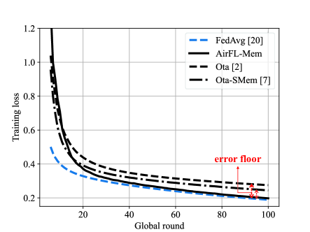
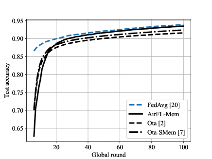
Figure 1: Training loss and test accuracy versus the number of communication rounds, $T$.

In this section, we evaluate the performance of AirFL-Mem in different setups with $K=20$ devices, with the aim of comparing its performance with benchmarks, as well as of showing the effectiveness of the proposed optimization of the truncation thresholds.

We consider the MNIST dataset learning task of classifying handwritten numbers, which is divided into $60,000$ training data samples and $10,000$ test data samples of $28\times 28$ images. The samples are drawn randomly (without replacement) from the training set to form the local data set. All devices train a common DNN model that consists of one input layer with input shape $(28,100)$, and one fully-connect layer of $100$ neurons, with ReLU activation function, and a softmax output layer, yielding a total number $d=79,510$ training parameters. SGD is adopted as an optimizer.

The simulation parameters are set as follows unless otherwise specified: the mini-batch size is $|\mathcal{D}_{k}^{(t)}|=64$; the number of local iterations $Q=1$; the power constraint $P_{k}=2\times 10^{-6}$ W; the AWGN variance $\sigma^{2}=-83$ dBm; the path loss $\kappa_{k}=c^{2}\mathord{\left/\right.\kern-1.2pt}\left(4\pi f_{c}r_{k}\right)^{2}$, where $c$ is the speed of light, $f_{c}=2.4$ GHz the central frequency, and $r_{k}$ the distance between device $k$ and edge server; the cell radius $100$ m, in which the devices are uniformly located $r_{k}\sim\mathcal{U}(0,100)$ and all devices are involved in training; and Rayleigh fading channel is considered. To perform the truncation threshold optimization, we determine the parameters $B=0.1$ and $L=0.1$ via numerical grid search.

We consider the following benchmarks: FedAvg with perfect communications [20]; the truncated channel inversion-based vanilla AirFL scheme [2], referred to as Ota; and AirFL with a short-term memory mechanism [7], which is referred to as Ota-SMem. The thresholds of Ota and Ota-SMem benchmarks are set the same as AirFL-Mem after optimization.

We first compare the training loss and test accuracy of the AirFL-Mem and benchmarks versus the communication round $T$, in Fig. 1. It is observed that the proposed AirFL-Mem approaches the ideal communication case, while Ota and Ota-SMem demonstrate significant error floors.

Finally, we compare the training loss versus the maximum transmit signal-to-noise ratio (SNR) in Fig. 2. For reference we also include the performance for a fixed threshold ($\epsilon=0.01$). The figure confirms that the proposed AirFL-Mem (with optimal thresholds) achieves performance close to FedAvg, as long as the SNR is large enough. In contrast, Ota and Ota-SMem suffer from error floors even in the range of significantly high transmit SNR.

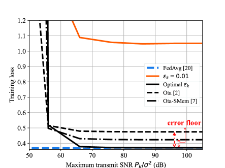
Figure 2: Training loss versus transmit SNR with $T=100$ iterations.

VII Conclusions

In this paper, we have proposed AirFL-Mem, an AirFL scheme that implements a long-term memory mechanism to mitigate the impact of deep fading. For non-convex objectives, we have provided convergence bounds that suggest that AirFL-Mem enjoys the same convergence rate as FedAvg with ideal communications, while existing schemes exhibit error floors. The analysis was also leveraged to introduce a novel convex optimization scheme for the optimization of power control thresholds. Experimental results have demonstrated the effectiveness of the proposed approach.

-A Sketch of the proof of Theorem IV.1

The proof of Theorem IV.1 hinges on the fact that the channel-induced sparsification $\mbox{\boldmath{$q$}}^{(t)}_{k}\odot(\bm{m}^{(t)}_{k}+\bm{\Delta}^{(t)}_{k})$ satisfies the contraction property as rand-$k$ [16], which is demonstrated by the following Lemma .1.

Lemma .1 (Truncated channel inversion as rand-$k$ contraction)

Under Assumption 4, for all $\mbox{\boldmath{$\theta$}}\in\mathbb{R}^{d\times 1}$, we have,

$$\mathbb{E}_{h}\left\|\mbox{\boldmath{$\theta$}}-\mbox{\boldmath{$q$}}_{k}^{(t)}\odot\mbox{\boldmath{$\theta$}}\right\|^{2}=(1-\lambda_{k})\|\mbox{\boldmath{$\theta$}}\|^{2},$$ (22)

where $\mathbb{E}_{h}[\cdot]$ is over the small-scale channel fading $h_{k,j}^{(t)}$’s.

Proof:

See Appendix -C. ∎

With the aid of Lemma .1, we have the following memory bound [17].

Lemma .2 (Bounded memory [17])

Under Assumption 2 and 4, for $\eta_{t}=\eta$, the expectation of the square norm of the long-term memory variable $\mbox{\boldmath{$m$}}_{k}^{(t)}$ for all $k\in[K]$ and $t\in[T]$, we have

$$\mathbb{E}\|\mbox{\boldmath{$m$}}_{k}^{(t)}\|^{2}\leq\frac{4(1-\lambda_{k}^{2})}{\lambda_{k}^{2}}\eta^{2}B^{2}Q^{2}.$$ (23)

Then we apply the perturbed iterate analysis as in [16] to provide the convergence bound of AirFL-Mem. Define the maintained virtual sequence $\{\tilde{\mbox{\boldmath{$\theta$}}}^{(t)}\}_{t=0,\ldots,T-1}$ as follows:

$$\tilde{\mbox{\boldmath{$\theta$}}}^{(t+1)}=\tilde{\mbox{\boldmath{$\theta$}}}^{(t)}-\mbox{\boldmath{$\Delta$}}^{(t)}-\frac{\eta^{(t)}}{\sqrt{\rho^{(t)}}K}\mbox{\boldmath{$n$}}^{(t)},$$ (24)

where $\mbox{\boldmath{$\Delta$}}^{(t)}=\frac{1}{K}\sum_{k=1}^{K}\mbox{\boldmath{$\Delta$}}_{k}^{(t)}$, and $\tilde{\mbox{\boldmath{$\theta$}}}^{(0)}=\mbox{\boldmath{$\theta$}}^{(0)}$. Then we have the following relations: with $\mbox{\boldmath{$m$}}_{k}^{(t+1)}=\bm{\Delta}^{(t)}_{k}+\mbox{\boldmath{$m$}}_{k}^{(t)}-\bm{q}^{(t)}_{k}\odot(\bm{\Delta}^{(t)}_{k}+\bm{m}^{(t)}_{k})$ and $\mbox{\boldmath{$m$}}_{k}^{(0)}=\mbox{\boldmath{$0$}}$, we have

$$\mathbb{E}\left\|\mbox{\boldmath{$\theta$}}^{(t)}-\tilde{\mbox{\boldmath{$\theta$}}}^{(t)}\right\|^{2}=\mathbb{E}\left\|\frac{1}{K}\sum_{k=1}^{K}\mbox{\boldmath{$m$}}_{k}^{(t)}\right\|^{2}\leq\frac{1}{K}\sum_{k=1}^{K}C_{\lambda_{k}}\eta^{2}B^{2}Q^{2},$$ (25)

where $C_{\lambda_{k}}=4(1-\lambda_{k}^{2})\mathord{\left/\right.\kern-1.2pt}\lambda_{k}^{2}$ and the inequality is followed by Jensen’s inequality and Lemma .2.

The proof of convergence of AirFL-Mem begins with the $L$-smoothness of gradient (Assumption 1). We first have

$$f\left(\tilde{\mbox{\boldmath{$\theta$}}}^{(t+1)}\right)\leq f\left(\tilde{\mbox{\boldmath{$\theta$}}}^{(t)}\right)-\left<\nabla f(\tilde{\mbox{\boldmath{$\theta$}}}^{(t)}),\mbox{\boldmath{$\Delta$}}^{(t)}+\frac{\eta^{(t)}}{\sqrt{\rho^{(t)}}K}\mbox{\boldmath{$n$}}^{(t)}\right>\\ +\frac{L}{2}\left\|\mbox{\boldmath{$\Delta$}}^{(t)}+\frac{\eta^{(t)}}{\sqrt{\rho^{(t)}}K}\mbox{\boldmath{$n$}}^{(t)}\right\|^{2}.$$ (26)

With some algebraic manipulations, for $\eta^{(t)}=\eta$, we arrive at (27) at the top of the next page.

$$\mathbb{E}\left[f\left(\tilde{\mbox{\boldmath{$\theta$}}}^{(t+1)}\right)\right]\leq f\left(\tilde{\mbox{\boldmath{$\theta$}}}^{(t)}\right)-\frac{\eta Q}{4}\left\|\nabla f(\mbox{\boldmath{$\theta$}}^{(t)})\right\|^{2}+\frac{3\eta QL^{2}}{2}\mathbb{E}\left\|\mbox{\boldmath{$\theta$}}^{(t)}-\tilde{\mbox{\boldmath{$\theta$}}}^{(t)}\right\|^{2}+\frac{\eta L^{2}}{K}\sum_{k=1}^{K}\sum_{q=0}^{Q-1}\mathbb{E}\left\|\mbox{\boldmath{$\theta$}}_{k}^{(t,q)}-\mbox{\boldmath{$\theta$}}^{(t)}\right\|^{2}+\frac{\eta^{2}\sigma^{2}Ld}{2K^{2}}\frac{1}{\rho^{(t)}}\\ +\frac{3}{K}\sum_{k=1}^{K}\mathbb{E}\left\|\sum_{q=0}^{Q-1}\tilde{\nabla}f_{k}(\mbox{\boldmath{$\theta$}}_{k}^{(t,q)})-\nabla f_{k}\left(\mbox{\boldmath{$\theta$}}_{k}^{(t,q)}\right)\right\|^{2}+\frac{3}{K}\sum_{k=1}^{K}\mathbb{E}\left\|\nabla f_{k}\left(\mbox{\boldmath{$\theta$}}_{k}^{(t,q)}\right)-\nabla f_{k}(\mbox{\boldmath{$\theta$}}_{k})\right\|^{2}+3Q^{2}\left\|\nabla f\left(\mbox{\boldmath{$\theta$}}^{(t)}\right)\right\|^{2}$$ (27)

To bound $1\mathord{\left/\right.\kern-1.2pt}\rho^{(t)}$, we introduce the following lemma.

Lemma .3

Under Assumption 2 and 4, we have

$$\frac{1}{\rho^{(t)}}\leq\max_{k\in[K]}\left\{\frac{2\lambda_{k}B^{2}Q^{2}(C_{\lambda_{k}}+1)}{dP_{k}\kappa_{k}\epsilon_{k}}\right\}.$$ (28)

Proof:

See Appendix -D. ∎

By applying the bound of $\mathbb{E}\|\mbox{\boldmath{$\theta$}}^{(t)}-\tilde{\mbox{\boldmath{$\theta$}}}^{(t)}\|^{2}$ in (25), Assumption 2-3, Lemma .2, Lemma 2 in [21], and Lemma .3, for $45\eta^{3}L^{3}Q^{3}+30\eta^{2}Q^{2}L^{2}+(3\mathord{\left/\right.\kern-1.2pt}2)\eta QL\leq 1\mathord{\left/\right.\kern-1.2pt}8$, we arrive at the inequality (29) at the top of the next page.

$$\mathbb{E}\left[f\left(\tilde{\mbox{\boldmath{$\theta$}}}^{(t+1)}\right)\right]\leq f\left(\tilde{\mbox{\boldmath{$\theta$}}}^{(t)}\right)-\frac{\eta Q}{8}\left\|\nabla f(\mbox{\boldmath{$\theta$}}^{(t)})\right\|^{2}+\frac{3\eta^{3}Q^{3}L^{2}B^{2}}{2}\frac{1}{K}\sum_{k=1}^{K}C_{\lambda_{k}}+\left(5\eta^{3}Q^{2}L^{2}+\frac{15}{2}\eta^{4}Q^{3}L^{3}\right)(\sigma_{l}^{2}+6Q\sigma_{g}^{2})\\ +\frac{3\eta^{2}LQ^{2}}{2}\sigma_{l}^{2}+\frac{\eta^{2}L}{K^{2}}\max_{k\in[K]}\left\{\frac{\lambda_{k}B^{2}Q^{2}(C_{\lambda_{k}}+1)}{P_{k}\kappa_{k}\epsilon_{k}}\right\}$$ (29)

Performing a telescopic sum from $t=0$ to $T-1$, taking an average over all randomness, putting the $\mathbb{E}\|\nabla f(\mbox{\boldmath{$\theta$}}^{(t)})\|^{2}$ to the left, and rearranging at (29), we obtain the inequality (19), which completes the proof of Theorem IV.1.

-B Convergence of AirFL with short-term memory and that without memory

We first consider the convergence of AirFL with short-term memory. Note that the global update is given by (9). By the $L$-smoothness of gradients, we have

$$f\left(\mbox{\boldmath{$\theta$}}^{(t+1)}\right)\leq f\left(\mbox{\boldmath{$\theta$}}^{(t)}\right)\\ -\left<\nabla f(\mbox{\boldmath{$\theta$}}^{(t)}),\frac{1}{K}\sum_{k=1}^{K}\mbox{\boldmath{$g$}}_{k}^{(t)}+\frac{\eta^{(t)}}{\sqrt{\rho^{(t)}}K}\mbox{\boldmath{$n$}}^{(t)}\right>\\ +\frac{L}{2}\left\|\frac{1}{K}\sum_{k=1}^{K}\mbox{\boldmath{$g$}}_{k}^{(t)}+\frac{\eta^{(t)}}{\sqrt{\rho^{(t)}}K}\mbox{\boldmath{$n$}}^{(t)}\right\|^{2}.$$ (30)

where $\mbox{\boldmath{$g$}}_{k}^{(t)}=\mbox{\boldmath{$q$}}_{k}^{(t)}\odot(\mbox{\boldmath{$\Delta$}}^{(t)}_{k}+\mbox{\boldmath{$m$}}^{\prime(t)}_{k})$. With some algebraic manipulations, we arrive at

$$\mathbb{E}\left[f\left(\mbox{\boldmath{$\theta$}}^{(t+1)}\right)\right]\leq f\left(\mbox{\boldmath{$\theta$}}^{(t)}\right)-\frac{\eta Q}{2}\left\|\nabla f(\mbox{\boldmath{$\theta$}}^{(t)})\right\|^{2}\\ +\frac{1}{\eta Q}\mathbb{E}\left\|\frac{1}{K}\sum_{k=1}^{K}\left(\mbox{\boldmath{$g$}}_{k}^{(t)}-\mbox{\boldmath{$\Delta$}}_{k}^{(t)}\right)\right\|^{2}+\frac{L}{2K}\sum_{k=1}^{K}\mathbb{E}\|\mbox{\boldmath{$g$}}_{k}^{(t)}\|^{2}\\ +\frac{\eta L^{2}}{K}\sum_{k=1}^{K}\sum_{q=0}^{Q-1}\mathbb{E}\left\|\mbox{\boldmath{$\theta$}}_{k}^{(t,q)}-\mbox{\boldmath{$\theta$}}^{(t)}\right\|^{2}+\frac{\eta^{2}\sigma^{2}Ld}{2K^{2}}\frac{1}{\rho^{(t)}},$$ (31)

which has the similar structure as (27). We bound the term $\mathbb{E}\left\|\mbox{\boldmath{$g$}}_{k}^{(t)}-\mbox{\boldmath{$\Delta$}}_{k}^{(t)}\right\|^{2}\leq 2(1-\lambda_{k}^{2})\eta^{2}Q^{2}B^{2}$ using Assumption 2 and 4; bound the term $\mathbb{E}\|\mbox{\boldmath{$\theta$}}_{k}^{(t,q)}-\mbox{\boldmath{$\theta$}}^{(t)}\|^{2}$ using Lemma 2 in [21]; and bound the term $\mathbb{E}\|\mbox{\boldmath{$g$}}_{k}^{(t)}\|^{2}\leq 2\lambda_{k}(2-\lambda_{k})\eta^{2}Q^{2}B^{2}$ using Assumption 2 and 4. Moreover, the bound of $1/\rho^{(t)}$ can be easily obtained by the bound of $\mathbb{E}\|\mbox{\boldmath{$g$}}_{k}^{(t)}\|^{2}$ followed by the steps in Appendix -D. Following the same strategy of Appendix -A, for proper choice of $\eta$, we easily obtain the final convergence result as

$$\frac{1}{T}\sum_{t=0}^{T-1}\mathbb{E}\|\nabla f(\bm{\theta}^{(t)})\|^{2}\leq\underbrace{\frac{4}{\eta QT}\left[f(\bm{\theta}^{(0)})-f^{*}\right]}_{\text{initilization error}}\\ +\underbrace{\frac{8B^{2}}{K}\sum_{k=1}^{K}C_{\lambda_{k}}}_{\text{contraction}}+\underbrace{\frac{4\eta L\sigma^{2}}{K^{2}}\max_{k\in[K]}\frac{\lambda_{k}B^{2}Q\tilde{C}_{\lambda_{k}}}{P_{k}\kappa_{k}\epsilon_{k}}}_{\text{effective channel noise}}\\ +20\eta^{2}L^{2}Q(\sigma_{l}^{2}+6Q\sigma_{g}^{2})+\frac{4\eta QB^{2}L}{K}\sum_{k=1}^{K}\lambda_{k}\tilde{C}_{\lambda_{k}},$$ (32)

where $C_{\lambda_{k}}=(1-\lambda_{k}^{2})$ and $\tilde{C}_{\lambda_{k}}=(2-\lambda_{k})$. This completes the convergence proof of AirFL with short-term memory.

For the convergence of AirFL without memory, we only need to change $\mbox{\boldmath{$g$}}_{k}^{(t)}$ to $\mbox{\boldmath{$g$}}_{k}^{(t)}=\mbox{\boldmath{$q$}}_{k}^{(t)}\odot\mbox{\boldmath{$m$}}^{\prime(t)}_{k}$ and follow the same steps, and then we can easily obtain the convergence result of AirFL without memory. Finally, we will obtain the same form as (32) with $C_{\lambda_{k}}=(1-\lambda_{k})$ and $\tilde{C}_{\lambda_{k}}=1/2$.

-C Proof of Lemma .1

For all $\mbox{\boldmath{$\theta$}}\in\mathbb{R}^{d\times 1}$, we have

$$\mathbb{E}_{h}\left\|\mbox{\boldmath{$\theta$}}-\mbox{\boldmath{$q$}}_{k}^{(t)}\odot\mbox{\boldmath{$\theta$}}\right\|^{2}$$ (33)

$$=\mathbb{E}_{h}\left\|\mbox{\boldmath{$\theta$}}\right\|^{2}-2\mathbb{E}_{h}\left<\mbox{\boldmath{$\theta$}},\mbox{\boldmath{$q$}}_{k}^{(t)}\odot\mbox{\boldmath{$\theta$}}\right>+\mathbb{E}_{h}\left\|\mbox{\boldmath{$q$}}_{k}^{(t)}\odot\mbox{\boldmath{$\theta$}}\right\|^{2}$$

$$\overset{(a)}{=}\mathbb{E}_{h}\left\|\mbox{\boldmath{$\theta$}}\right\|^{2}-\mathbb{E}_{h}\left\|\mbox{\boldmath{$q$}}_{k}^{(t)}\odot\mbox{\boldmath{$\theta$}}\right\|^{2},$$

where (a) is due to $\left<\mbox{\boldmath{$\theta$}},\mbox{\boldmath{$q$}}_{k}^{(t)}\odot\mbox{\boldmath{$\theta$}}\right>=\|\mbox{\boldmath{$q$}}_{k}^{(t)}\odot\mbox{\boldmath{$\theta$}}\|^{2}$. Then we calculate the term $\mathbb{E}_{h}\|\mbox{\boldmath{$q$}}_{k}^{(t)}\odot\mbox{\boldmath{$\theta$}}\|^{2}$ as follows.

$$\mathbb{E}_{h}\left\|\mbox{\boldmath{$q$}}_{k}^{(t)}\odot\mbox{\boldmath{$\theta$}}\right\|^{2} =\mathbb{E}_{h}\left[\sum_{m=1}^{d}|\theta_{m}|^{2}q_{k,j}^{(t)}\right]$$ (34)

$$=\sum_{m=1}^{d}\left(|\theta_{m}|^{2}\mathbb{E}_{h}\left[q_{k,j}^{(t)}\right]\right)=\lambda_{k}\|\mbox{\boldmath{$\theta$}}\|^{2},$$

which yields the desired result.

-D Proof of Lemma .3

Record that the power constraint for all $k\in[K]$ is given by

$$\frac{1}{d}\mathbb{E}\left\|\mbox{\boldmath{$p$}}_{k}^{(t)}\odot\mbox{\boldmath{$q$}}_{k}^{(t)}\odot\bm{x}_{k}^{(t)}\right\|^{2}\leq P_{k},$$ (35)

where $\mbox{\boldmath{$x$}}_{k}^{(t)}=(\bm{\Delta}^{(t)}_{k}+\bm{m}^{(t)}_{k})/\eta^{(t)}$ for AirFL-Mem. By (6), we can obtain

$$\mathbb{E}\left\|\mbox{\boldmath{$p$}}_{k}^{(t)}\odot\mbox{\boldmath{$q$}}_{k}^{(t)}\odot\bm{x}_{k}^{(t)}\right\|^{2}$$ (36)

$$=\frac{\rho^{(t)}}{\kappa_{k}\eta^{2}}\mathbb{E}\left[\sum_{j=1}^{d}\left(\frac{q_{k,j}^{(t)}}{|h_{k,j}^{(t)}|^{2}}\left(\Delta^{(t)}_{k,j}+m^{(t)}_{k,j}\right)^{2}\right)\right]$$

$$\leq\frac{\rho^{(t)}}{\kappa_{k}\epsilon_{k}\eta^{2}}\mathbb{E}\left[\sum_{j=1}^{d}\left(q_{k,j}^{(t)}\left(\Delta^{(t)}_{k,j}+m^{(t)}_{k,j}\right)^{2}\right)\right]$$

$$=\frac{\rho^{(t)}}{\kappa_{k}\epsilon_{k}\eta^{2}}\sum_{j=1}^{d}\left(\mathbb{E}[q_{k,j}^{(t)}]\mathbb{E}\left[\left(\Delta^{(t)}_{k,j}+m^{(t)}_{k,j}\right)^{2}\right]\right)$$

$$=\frac{\rho^{(t)}\lambda_{k}}{\kappa_{k}\epsilon_{k}\eta^{2}}\mathbb{E}\|\mbox{\boldmath{$\Delta$}}^{(t)}_{k}+\mbox{\boldmath{$m$}}^{(t)}_{k}\|^{2}$$

$$\leq\frac{\rho^{(t)}\lambda_{k}}{\kappa_{k}\epsilon_{k}\eta^{2}}(2\mathbb{E}\|\mbox{\boldmath{$\Delta$}}^{(t)}_{k}\|^{2}+2\mathbb{E}\|\mbox{\boldmath{$m$}}^{(t)}_{k}\|^{2})$$

$$\leq\underbrace{\frac{\rho^{(t)}\lambda_{k}}{\kappa_{k}\epsilon_{k}}2B^{2}Q^{2}(C_{\lambda_{k}}+1)}_{A(\rho^{(t)})}.$$

where the last inequality is followed by Assumption 2 and Lemma .2. We choose $\tilde{\rho}$ such that $A(\tilde{\rho})\leq dP_{k}$ for all $k\in[K]$ is satisfied, i.e.,

$$\tilde{\rho}\triangleq\min_{k\in[K]}\frac{dP_{k}\kappa_{k}\epsilon_{k}}{2\lambda_{k}B^{2}Q^{2}(C_{\lambda_{k}}+1)}.$$ (37)

By the long-term power constraint and the definition of $\tilde{\rho}$, we have $\rho^{(t)}\geq\tilde{\rho}$, i.e.,

$$\frac{1}{\rho^{(t)}}\leq\frac{1}{\tilde{\rho}}=\max_{k\in[K]}\frac{2\lambda_{k}B^{2}Q^{2}(C_{\lambda_{k}}+1)}{dP_{k}\kappa_{k}\epsilon_{k}},$$ (38)

which yields the desired result.

-E Proof of Proposition V.1

Define functions $g(x)=a\left(1-x^{2}\right)\mathord{\left/\right.\kern-1.2pt}x^{2}$ and $f_{k}(x)=b_{k}\left(4\left(1-x^{2}\right)\mathord{\left/\right.\kern-1.2pt}x+x\right)\mathord{\left/\right.\kern-1.2pt}\log\left(\frac{1}{x}\right)$, where $a$ and $b_{k}$ are some constants, and $\text{dom}f=\text{dom}g=(0,1)$. The function $f(x)$ is convex since

$$f_{k}^{\prime\prime}(x)=\frac{b_{k}\left(\frac{8\left(\log^{2}\left(\frac{1}{x}\right)+1\right)}{x^{3}}+\left(-\frac{12}{x^{3}}-\frac{3}{x}\right)\log\left(\frac{1}{x}\right)-\frac{6}{x}\right)}{\log^{3}\left(\frac{1}{x}\right)}$$ (39)

is positive in $0<x<1$. And $g(x)$ is convex since $g^{\prime\prime}(x)=6a\mathord{\left/\right.\kern-1.2pt}x^{4}>0$ for all $0<x<1$. Then we use the fact that the finite sum of convex functions is convex and $\max_{k}f_{k}$ is convex when $f_{k}$ is convex, which yields the objective in Problem $\mathrm{(P2)}$ is convex in $(0,1)$.

References

• [1] B. Nazer and M. Gastpar, “Computation over multiple-access channels,” IEEE Transactions on information theory, vol. 53, no. 10, pp. 3498–3516, 2007.
• [2] G. Zhu, Y. Wang, and K. Huang, “Broadband analog aggregation for low-latency federated edge learning,” IEEE Trans. Wireless Commun., vol. 19, no. 1, pp. 491–506, 2020.
• [3] T. Sery, N. Shlezinger, K. Cohen, and Y. C. Eldar, “Over-the-air federated learning from heterogeneous data,” IEEE Trans. Signal Process., vol. 69, pp. 3796–3811, 2021.
• [4] X. Cao, G. Zhu, J. Xu, Z. Wang, and S. Cui, “Optimized power control design for over-the-air federated edge learning,” IEEE J. Sel. Areas Commun., vol. 40, no. 1, pp. 342–358, 2021.
• [5] S. M. Shah, L. Su, and V. K. Lau, “Robust federated learning over noisy fading channels,” Internet Things J., vol. 10, no. 9, pp. 7993–8013, 2022.
• [6] J. Yao, Z. Yang, W. Xu, D. Niyato, and X. You, “Imperfect CSI: A key factor of uncertainty to over-the-air federated learning,” arXiv preprint arXiv:2307.12793, 2023.
• [7] M. M. Amiri and D. Gündüz, “Federated learning over wireless fading channels,” IEEE Trans. Wireless Commun., vol. 19, no. 5, pp. 3546–3557, 2020.
• [8] T. Sery and K. Cohen, “On analog gradient descent learning over multiple access fading channels,” IEEE Trans. Signal Process., vol. 68, pp. 2897–2911, 2020.
• [9] R. Paul, Y. Friedman, and K. Cohen, “Accelerated gradient descent learning over multiple access fading channels,” IEEE J. Sel. Areas Commun., vol. 40, no. 2, pp. 532–547, 2021.
• [10] K. Yang, T. Jiang, Y. Shi, and Z. Ding, “Federated learning via over-the-air computation,” IEEE Trans. Wireless Commun., vol. 19, no. 3, pp. 2022–2035, 2020.
• [11] S. Xia, J. Zhu, Y. Yang, Y. Zhou, Y. Shi, and W. Chen, “Fast convergence algorithm for analog federated learning,” in Proc. ICC 2021 - IEEE International Conference on Communications, Montreal, QC, Canada, 2021, pp. 1–6.
• [12] M. M. Amiri, T. M. Duman, D. Gündüz, S. R. Kulkarni, and H. V. Poor, “Blind federated edge learning,” IEEE Trans. Wireless Commun., vol. 20, no. 8, pp. 5129–5143, 2021.
• [13] H. H. Yang, Z. Chen, T. Q. Quek, and H. V. Poor, “Revisiting analog over-the-air machine learning: The blessing and curse of interference,” IEEE J Sel. Top. Signal Process., vol. 16, no. 3, pp. 406–419, 2021.
• [14] X. Wei, C. Shen, J. Yang, and H. V. Poor, “Random orthogonalization for federated learning in massive mimo systems,” IEEE Trans. Wireless Commun., 2023.
• [15] B. Tegin and T. M. Duman, “Federated learning with over-the-air aggregation over time-varying channels,” IEEE Trans. Wireless Commun., 2023.
• [16] S. U. Stich, J.-B. Cordonnier, and M. Jaggi, “Sparsified SGD with memory,” Advances in Neural Information Processing Systems, vol. 31, 2018.
• [17] D. Basu, D. Data, C. Karakus, and S. Diggavi, “Qsparse-local-SGD: Distributed SGD with quantization, sparsification and local computations,” in Proc. Advances in Neural Information Processing Systems (NeurIPS), Vancouver, Canada, Dec. 2019.
• [18] S. P. Karimireddy, Q. Rebjock, S. Stich, and M. Jaggi, “Error feedback fixes signsgd and other gradient compression schemes,” in Proc. International Conference on Machine Learning.   PMLR, 2019, pp. 3252–3261.
• [19] J. Yun, Y. Oh, Y.-S. Jeon, and H. V. Poor, “Communication-efficient federated learning over capacity-limited wireless networks,” arXiv preprint arXiv:2307.10815, 2023.
• [20] B. McMahan, E. Moore, D. Ramage, S. Hampson, and B. A. y Arcas, “Communication-efficient learning of deep networks from decentralized data,” in Proc. Artificial intelligence and statistics.   PMLR, 2017, pp. 1273–1282.
• [21] H. Yang, M. Fang, and J. Liu, “Achieving linear speedup with partial worker participation in non-iid federated learning,” in Proc. International Conference on Learning Representations (ICLR), 2021.
• [22] S. Boyd and L. Vandenberghe, Convex Optimization.   Cambridge Univ. Press, 2004.
• [23] M. Grant and S. Boyd, “CVX: Matlab software for disciplined convex programming, version 2.1,” Mar. 2014. [Online]. Available: http://cvxr.com/cvx