Certifying Bimanual RRT Motion Plans in a Second

Abstract

We present an efficient method for certifying non-collision for piecewise-polynomial motion plans in algebraic reparametrizations of configuration space. Such motion plans include those generated by popular randomized methods including RRTs and PRMs, as well as those generated by many methods in trajectory optimization. Based on Sums-of-Squares optimization, our method provides exact, rigorous certificates of non-collision; it can never falsely claim that a motion plan containing collisions is collision-free. We demonstrate that our formulation is practical for real world deployment, certifying the safety of a twelve degree of freedom motion plan in just over a second. Moreover, the method is capable of discriminating the safety or lack thereof of two motion plans which differ by only millimeters.

I Introduction

Collision-free motion planning is a fundamental problem in the safe and efficient operation of any robotic system. One of the most important subroutines in collision-free motion planning is collision detection, which has been studied extensively in robotics [cameron1985study, he2014efficient], computer graphics [lin1998collision, hubbard1995collision], and computational geometry more broadly [shamos1976geometric, lin2017collision]. Algorithms for checking whether a single configuration is collision free are quite mature and can be performed in microseconds on modern hardware [pan2012fcl].

By contrast, algorithms which are capable of certifying non-collision for the infinite family of configurations along a motion plan are less common. Known as dynamic collision checking, this subroutine is performed hundreds to thousands of times in randomized motion planning methods, and so the speed as well as the correctness of these algorithms is central to their adoption. Due to the speed requirement, it is common practice to heuristically perform dynamic collision checking by sampling a finite number of static configurations along the motion plan. Nevertheless, it is widely recognized that this is insufficient for safety critical robots.

This has motivated a number of more sophisticated algorithms for certifying the safety along a motion plan. These broadly fall into three major families: feature tracking, swept volumes, and trajectory parametrization methods [jimenez20013d].

Both the feature tracking and swept volume methods have effectively scaled to applications in both graphics and robotics. The most successful methods rely on pre-computing a hierarchy of bounding volumes at various resolutions and certifying non-intersection at a finite number of points along the motion plan [jackins1980oct]. The choice of samples is done in an adaptive manner which guarantees non-collision and some algorithms are fast enough for use as dynamic collision checkers during randomized motion planning [schwarzer2004exact].

These methods have two primary drawbacks. The first is that they frequently only consider piecewise linear configuration space motion plans and so cannot generalize to smoother plans. The second drawback can be their conservativeness. Typically, these methods require difficult-to-compute parameters such as an upper bound on the maximum length of a curve along the swept volume [schwarzer2004exact] or bounding the rate of change of the distance between two objects over the course of the trajectory [zhang2007continuous]. If these bounds are too loose, collision-free motion plans in tight configuration spaces cannot be certified, which is arguably the most important regime.

On the other hand, trajectory parametrizaton methods can certify any collision-free motion plan to arbitrary precision. This is because these methods make relatively minimal assumptions to obtain exact guarantees, requiring only knowledge of the forward kinematics of the robot and a concrete, description of the collision geometries [canny1986collision], [schweikard1991polynomial]. Both are often necessary information for the simulation of any robotic system and so are readily available. However, most of these methods rely on exact, algebraic computations such as polynomial root finding, and so are typically too slow for practical deployment.

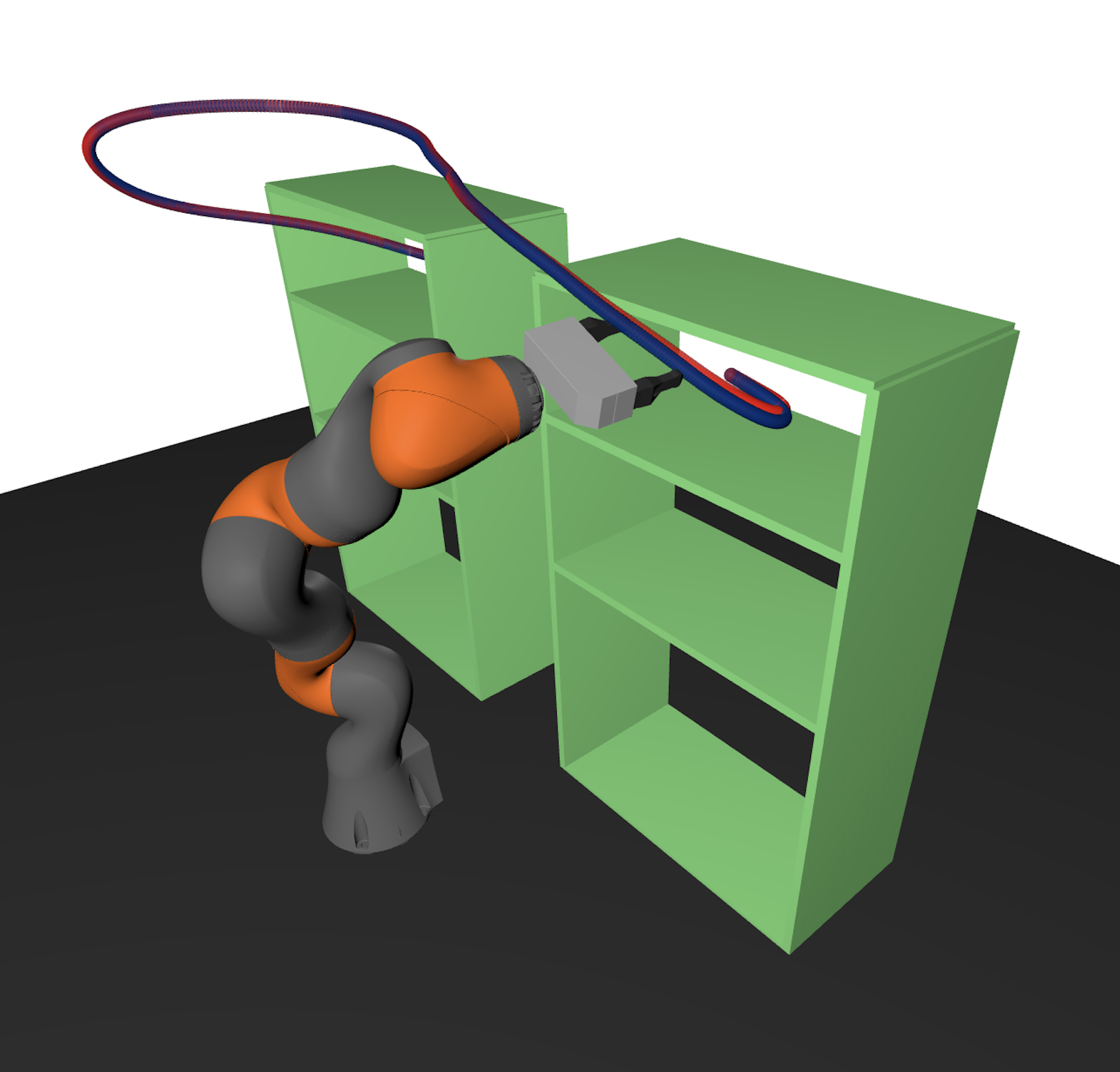
Figure 1: A 7-DOF Kuka iiwa reaching into a pair of shelves. Despite being visually indistinguishable, the blue motion plan is collision-free, while the red motion plan contains minor collision when reaching into each shelf. The proposed certification method is capable of discriminating the safety of these two motion plans.

I-A Contribution

This paper presents a certification method in the family of trajectory parametrization algorithms which is efficient enough for practical deployment on robotic systems. In particular, we employ sums-of-squares (SOS) optimization to provide a rigorous method for certifying motion plans parametrized by polynomials of arbitrary degree.

Our method specializes a technique for certifying non-collision in full-dimensional volumes of configuration space presented in [dai2023certified]. By restricting ourselves to planned motion case, we are able to leverage stronger results in optimization and dramatically reduce computation times.

We deploy our method to certify a piecewise-cubic motion plan for a 7-DOF arm, and a rapidly-exploring random tree (RRT) for a 12-DOF, bimanual manipulation example. As seen in Figure 1, we demonstrate that our method is capable of discriminating between safe and unsafe motion plans which are arbitrarily close together and can be used to certify that a pair of geometries do not collide along a motion plan in at most hundreds of milliseconds. The result is a certifier which can verify the safety of arbitrarily complicated polynomial motion plans in a handful of seconds, or piecewise-linear plans from an RRT in a second.

I-B Notation

Throughout, we use calligraphic letters ($\mathcal{X}$) to denote sets, Roman capitals ($X$) to denote matrices, and Roman lower case ($x$) to denote vectors or scalars. We use $X\succeq 0$ to denote that a symmetric matrix $X$ belongs to the cone of positive semidefinite (PSD) matrices which are denoted as $\mathbb{S}_{+}$ .

For a vector $x$ of $m$ variables, we denote by $[x]_{d}\coloneqq\begin{bmatrix}1,x_{1},\dots,x_{m},x_{1}^{2},x_{1}x_{2},\dots,x_{m}^{d}\end{bmatrix}^{T}$ the vector of all ${{m+d}\choose d}$ monomials in $x_{1},\dots,x_{m}$ of degree less than or equal to $d$. The vector space of real polynomials in $x$ of degree $d$ is written as $\mathbb{R}[x]_{d}$ while $n\times k$ matrices with entries in $\mathbb{R}[x]_{d}$ is are written as $\mathbb{R}[x]^{n\times k}_{d}$. If $d$ is omitted, then $\mathbb{R}[x]$ and $\mathbb{R}[x]^{n\times k}$ are the set of all polynomials of arbitrary degree.

Finally, for $p(x)\in\mathbb{R}[x]$ we denote by $\deg_{x_{i}}(p)$ the degree of the polynomial $p$ in the variable $x_{i}$ and similarly $\deg_{x_{i}}(P)=\displaystyle{\max_{i,j}}\ \deg(P_{i,j}(x))$ for $P(x)\in\mathbb{R}[x]_{d}^{n\times k}$. When the variable is clear, the subscript is suppressed.

II Mathematical Preliminaries

In this section, we introduce the essential mathematical ingredients which we will leverage to provide efficient certification of non-collision along our robot motion plans. Our method relies on well-known results from convex optimization [boyd2004convex], methods from sums-of-squares programming [blekherman2012semidefinite, Chapter 3], and an algebraic reparametrization of the forward kinematics [wampler2011numerical].

II-A Separating Convex Bodies

Figure 2: The closed, convex bodies $\mathcal{A}$ and $\mathcal{B}$ are collision-free if and only if there exists a hyperplane $a^{T}x+b=0$ separating the two. As the bodies move in space, a different hyperplane may be needed to certify their non-collision.

A well-known result from convex optimization is the Separating Hyperplane Theorem [boyd2004convex], which states that two closed, convex bodies $\mathcal{A}$ and $\mathcal{B}$ do not intersect if and only there exists a hyperplane $a^{T}x+b=0$ separating the bodies such as in Figure 2. The search for such a hyperplane can be posed as the optimization program:

$$\textbf{Find }~{}a,b~{}\operatorname{\textbf{subject\ to}}$$ (1a)

$$a^{T}x+b>0,~{}\forall x\in\mathcal{A}$$ (1b)

$$a^{T}x+b<0,~{}\forall x\in\mathcal{B}$$ (1c)

which is convex since $\mathcal{A}$ and $\mathcal{B}$ are convex sets. The hyperplane $\mathcal{H}=\{x\mid a^{T}x+b=0\}$ serves as a rigorous, mathematical proof that $\mathcal{A}$ and $\mathcal{B}$ do not intersect, and so we refer to $\mathcal{H}$ as a separation certificate.

Example 1

If $\mathcal{A}$ is a polytope with vertices $\{v_{1},\dots,v_{N}\}$, we can express (1b) using $N$ linear constraints:

$$a^{T}v_{i}+b\geq 1~{}\forall i\in\{1,\dots,N\}.$$

Example 2

If $\mathcal{A}$ is a sphere with center $c$ and radius $r$, we can express (1b) using the PSD constraint:

$$\begin{bmatrix}(a^{T}c+b)I&ra\\ ra^{T}&a^{T}c+b\end{bmatrix}\succeq 0$$

Further explicit examples of expressing (1b) are available in [dai2023certified].

II-B Polynomial Positivity on Intervals

Our method in Section IV will rely on a generalization of (1) that was first introduced in [amice2022finding, dai2023certified]. This generalization relies heavily on the ability to certify that certain polynomials (resp. matrices) are non-negative (resp. positive semidefinite). Unlike in [amice2022finding, dai2023certified], our polynomials will be univariate and so we will be able to leverage much stronger theory than this prior work.

We begin by recalling the definition of a Sums-of-Squares (SOS) polynomial and a SOS matrix [blekherman2012semidefinite].

Definition 1

A polynomial $p(x)\in\mathbb{R}[x]_{2d}$ is sums-of-squares if it can be expressed as $p(x)=\sum_{i=1}^{N}q_{i}^{2}(x)$ for $q_{i}\in\mathbb{R}[x]_{d}$. Equivalently, $p(x)$ is SOS if it can be expressed as $[x]_{d}^{T}Q[x]_{d}$ for $Q\succeq 0$. The set of all SOS polynomials of degree $2d$ is denoted $\Sigma[x]_{2d}$.

A similar notion exists for SOS matrices.

Definition 2

A symmetric matrix $P(x)\in\mathbb{R}[x]_{2d}^{n\times n}$ is a SOS matrix if there exists a polynomial matrix $\Theta(x)\in\mathbb{R}[x]_{d}^{k\times n}$ such that $P(x)=\Theta(x)^{T}\Theta(x)$. The set of all $n\times n$ SOS matrices of degree $2d$ is denoted $\Sigma[x]^{n\times n}_{2d}$.

A useful characterization relating SOS matrices to SOS polynomials is given by the following theorem.

Theorem 1 ([blekherman2012semidefinite], Lemma 3.78)

Let $P(x)\in\mathbb{R}[x]_{2d}^{n\times n}$ be a symmetric polynomial matrix and let $y=\begin{bmatrix}y_{1}&\dots&y_{n}\end{bmatrix}$ be a vector of monomials. Define the scalar polynomial $p(x,y)=y^{T}P(x)y$. Then $P(x)$ is a SOS matrix if and only if $p(x,y)$ is SOS.

The characterization of SOS polynomials and matrices in terms of the existence of a semidefinite matrix $Q$ is attractive as it allows one to search for certificates of non-negativity using convex optimization, specifically semidefinite programming (SDP) [parrilo2000structured]. This is known as SOS programming.

Finally, we recall two very strong theorems about the non-negativity of univariate polynomials and polynomial matrices on intervals.

Theorem 2 (Markov-Lucasz [roh2006discrete])

A univariate polynomial $p(x)$ is non-negative on the non-empty interval $x\in[a,b]$ if and only if it can be expressed as

$$p(x)=\begin{cases}\lambda(x)+(x-a)(b-x)\nu(x),&\deg(p)=2d\\ (x-a)\lambda(x)+(b-x)\nu(x),&\deg(p)=2d+1\end{cases}$$ (2)

where $\lambda,~{}\nu\in\bm{\Sigma}[x]$. Moreover, if $d=\left\lfloor\frac{\deg(p)}{2}\right\rfloor$ then

$$\deg(\lambda)\leq 2d,~{}~{}\deg(\nu)\leq\begin{cases}2d-2&\text{if }\deg(p)=2d\\ 2d&\text{if }\deg(p)=2d+1\end{cases}.$$ (3)

An analogous theorem holds in the univariate matrix case.

Theorem 3

Let $P(x)\in\mathbb{R}[x]^{m\times m}$ be a symmetric matrix of univariate polynomials. Then $P(x)\succeq 0$ on the non-empty interval $x\in[a,b]$ if and only if $p(x,y)=y^{T}P(x)y$ can be expressed as:

$$p(x,y)=\begin{cases}\lambda(x,y)+(x-a)(b-x)\nu(x,y),&\deg(P)=2d\\ (x-a)\lambda(x,y)+(b-x)\nu(x,y),&\deg(P)=2d+1\end{cases}$$ (4)

where $\lambda,~{}\nu\in\bm{\Sigma}[x,y]$. Moreover, if $d=\left\lfloor\frac{\deg(P)}{2}\right\rfloor$ then

$$\begin{gathered}\deg_{y_{i}}(\lambda)=2,~{}\deg_{y_{i}}(\nu)=2,~{}\deg_{x}(\lambda)\leq 2d\\ \deg_{x}(\nu)\leq\begin{cases}2d-2&\text{if }\deg(P)=2d\\ 2d&\text{if }\deg(P)=2d+1\end{cases}\end{gathered}.$$ (7)

Proof.

This follows by applying a similar argument as used in [roh2006discrete] to prove Theorem 2 to the matrix $P(x)$ and leveraging the result of [choi1980real] that univariate PSD matrices are always SOS matrices. ∎

The polynomials $\lambda$ and $\nu$ in Theorems 2 and 3 are traditionally referred to as multiplier polynomial and serve as a certificate of non-negativity on the interval $[a,b]$.

Remark 1

Analogs of Theorems 2 and 3 exist when the polynomials are allowed to be multivariate and are leveraged in [amice2022finding, dai2023certified]. The main advantage to restricting to the univariate case is the explicit degree bounds on the multiplier polynomials which are not available in the multivariate case.

II-C Algebraic Forward Kinematics

Our approach in Section IV will rely critically on a polynomial parametrization of the forward kinematics of a robot.

Definition 3

A rigid-body robot is called algebraic if all links are connected by a composition of the following two joints:

• Revolute (R): a 1-DOF joint permitting revolution about an axis. An example is a door hinge.

• Prismatic (P): a 1-DOF joint permitting translation along an axis. An example is a linear rail.

In addition to (R) and (P) joints, many common joints such as cylindrical, planar, and spherical joints can be represented as a composition of R and P joints [wampler2011numerical].

In general, the forward kinematics of an algebraic robot can be expressed as multilinear trigonometric polynomials [wampler2011numerical]. Concretely, using the monogram notation from [tedrakeManip], the $w$^th component (for $w\in\{x,y,z\}$) of the position of a point $A$ relative to a frame $F$ and expressed in $F$ is can be written as:

$$\leftidx{{}^{F}}p^{A}_{w}(q)=\sum_{j}c_{jw}\prod_{i}\xi_{ij,w}(q_{i})$$

where $c_{jw}$ are constant coefficients and $\xi_{ij,w}(q_{i})\in\{\cos(\theta_{i}),\sin(\theta_{i})\}$ if the $i$^th joint is associated to an (R) joint or $\xi_{ij,w}(q_{i})=z_{i}$ if the $i$^th joint is associated to a (P) joint. The collection of variables $q=\cup_{i}\{\theta_{i},z_{i}\}$ are referred to as the configuration-space (C-space) variables.

While (II-C) is not a polynomial due to the presence of the trigonometric functions $\sin(q_{i})$ and $\cos(q_{i})$, it admits a rational reparametrization.

Definition 4

Define the substitution $\tau_{i}\coloneqq\tan\left(\frac{\theta_{i}}{2}\right)$. This substitution implies that

$$\cos(\theta_{i})=\frac{1-\tau_{i}^{2}}{1+\tau_{i}^{2}},~{}~{}~{}\sin(\theta_{i})=\frac{2\tau_{i}^{2}}{1+\tau_{i}^{2}}.$$

The collection of variables $s=\cup_{i}\{\tau_{i},z_{i}\}$ are referred to as the tangential-configuration space (TC-space) variables.

This substitution is known as the stereographic projection [spivakCalc] and is bijective for $\theta_{i}\in(-\pi,\pi)$. Under this substitution, (II-C) can be expressed as an rational function with a positive, polynomial denominator:

$$\leftidx{{}^{F}}p^{A}_{w}(s)=\sum_{j}c_{jw}\prod_{i\in\mathcal{I}_{F,A}}\frac{\leftidx{{}^{F}}f_{ij,w}^{A}(s_{i})}{\leftidx{{}^{F}}g_{ij,w}^{A}(s_{i})}=\frac{\leftidx{{}^{F}}f^{A}_{w}(s)}{\leftidx{{}^{F}}g^{A}_{w}(s)}$$ (8)

where

$$\frac{\leftidx{{}^{F}}f_{ij,w}^{A}(s_{i})}{\leftidx{{}^{F}}g_{ij,w}^{A}(s_{i})}\in\left\{\frac{1-\tau_{i}^{2}}{1+\tau_{i}^{2}},\frac{2\tau_{i}}{1+\tau_{i}^{2}},\frac{z_{i}}{1}\right\}.$$

Example 3

We consider the forward kinematics of a pendulum mounted on a moving rail shown in Figure 3. Letting $z$ denote the commanded position from the left wall, and $\theta$ the angle from the vertical, the position $(p_{x},p_{y})$ of the tip of the pendulum in C-space and TC-space coordinates is:

	C-space	TC-space
$p_{x}$	$\displaystyle{l_{1}\sin(\theta)+z}$	$\displaystyle{l_{1}\left(\frac{2\tau}{1+\tau^{2}}\right)+z}$
$p_{y}$	$\displaystyle{l_{1}\cos(\theta)}$	$\displaystyle{l_{1}\left(\frac{1-\tau^{2}}{1+\tau^{2}}\right)}$

Figure 3: The pendulum on rail system.

Notice that the stereographic projection does induce some warping of distances in configuration space. However, in the limited joint range of many standard industrial manipulators, this warping is minor and straight lines in TC-space are approximately straight lines in C-space.

Remark 2

An alternative reparametrization of (II-C) introduces the substitutions $\sigma_{i}\coloneqq\sin(\theta_{i})$ and $c_{i}\coloneqq\cos(\theta_{i})$ with the constraint that $\sigma_{i}^{2}+c_{i}^{2}=1$ and is known as the algebraic-configuration space (AC-space). All results in this paper are easily extended to AC-space with no change in the underlying mathematics. We prefer to use TC-space throughout as it is easier to generate feasible motion plans.

III Problem Formulation

We consider an algebraic, rigid-body robot operating in a known environment. The geometry of the robot and all obstacles in the environment are assumed to have a known decomposition as a union of compact, convex bodies such as spheres, capsules, cylinders, or polytopes. Such collision geometries of our task space are readily available through standard tools such as V-HACD [mamou2009simple] and are often a required step for simulating any given environment. We refer to the pairs of bodies which can collide as the collision pairs. Under these assumption, we introduce the following problem.

Notice that solving PlanCert also covers the case when the plan $\rho$ is a piecewise polynomial, as we can simply certify each piecewise segment individually.

Remark 3

Finitely sampling for collisions along the plan is an algorithm with false optimism. It can return safe when the plan does in fact contain collisions. Our preference is for an algorithm which may sometimes declare a segment is NotSafe when it is in fact safe , but only declares safe when the plan is in fact safe.

IV Proving Non-collision along a Plan

In this section, we provide an efficient solution to PlanCert based on convex optimization, specifically SOS programming. Our method is based on generalizing (1) to handle a motion plan $\rho(t)$ of configurations.

Let $\mathcal{A}(s)$ denote the position of the convex body $\mathcal{A}$ at the TC-space configuration $s$. Recall from Section II-C that we can express any point $x(s)\in\mathcal{A}(s)$ as a rational function with a positive denominator and so $x(\rho(t))$ for $t\in[0,1]$ is again a rational function with a positive denominator (rational functions are closed under composition with polynomials).

Now, as the position of two bodies $\mathcal{A}(t)\coloneqq\mathcal{A}(\rho(t))$ and $\mathcal{B}(t)\coloneqq\mathcal{B}(\rho(t))$ vary over the motion plan, a single, static hyperplane may be insufficient to certify that $\mathcal{A}(t)$ and $\mathcal{B}(t)$ do not collide as in Figure 2. Therefore, we allow the hyperplane parameters $a$ and $b$ to also vary as a polynomial function of $t$.

For every pair of bodies $(\mathcal{A}(t),\mathcal{B}(t))$ which can collide in the environment, we search for a polynomially parametrized family of hyperplanes $(a_{\mathcal{A},\mathcal{B}}(t),b_{\mathcal{A},\mathcal{B}}(t))$ which certify that $(\mathcal{A}(t),\mathcal{B}(t))$ do not collide for $t\in[0,1]$. Concretely:

$${\forall~{}\text{pairs }\mathcal{A},\mathcal{B}}$$

$$~{}\textbf{Find }a_{\mathcal{A},\mathcal{B}}(t),b_{\mathcal{A},\mathcal{B}}(t)~{}~{}\textbf{subject to}$$ (12a)

$$\begin{rcases}a^{T}_{\mathcal{A},\mathcal{B}}(t)x(t)+b_{\mathcal{A},\mathcal{B}}(t)>0,~{}\forall x\in\mathcal{A}(t)\\ a^{T}_{\mathcal{A},\mathcal{B}}(t)x(t)+b_{\mathcal{A},\mathcal{B}}(t)<0,~{}\forall x\in\mathcal{B}(t)\end{rcases}\forall t\in[0,1].$$ (12b)

This is an optimization program over polynomials which can be solved using SDP by transforming (12b) into equivalent linear and semidefinite constraints using Theorems 2 and 3. A feasible solution to (12) is a collection of polynomials

$$\mathcal{C}=\bigcup_{\mathcal{A},\mathcal{B}}\left\{a_{\mathcal{A},\mathcal{B}},b_{\mathcal{A},\mathcal{B}},\lambda_{\mathcal{A}},\nu_{\mathcal{A}},\lambda_{\mathcal{B}},\nu_{\mathcal{B}},\right\}$$

and is a certificate of non-collision. At every time point $t\in[0,1]$, the polynomials $(a_{\mathcal{A},\mathcal{B}}(t),b_{\mathcal{A},\mathcal{B}}(t))$ serve as a separation certificate for $(\mathcal{A}(t),\mathcal{B}(t))$. Meanwhile $\{\lambda_{\mathcal{A}},\nu_{\mathcal{A}},\lambda_{\mathcal{B}},\nu_{\mathcal{B}}\}$ serve as a certificate of positivity that $(a_{\mathcal{A},\mathcal{B}}(t),b_{\mathcal{A},\mathcal{B}}(t))$ are a separation certificate for every ${t\in[0,1]}$.

Example 4

If $\mathcal{A}(t)$ is a polytope with vertices $v_{i}$ at positions $\leftidx{{}^{F}}p^{v_{i}}(t)=\frac{\leftidx{{}^{F}}f^{v_{i}}(\rho(t))}{\leftidx{{}^{F}}g^{v_{i}}(\rho(t))}$ for $i\in\{1,\dots,N\}$, then we can enforce (12b) using $N$ polynomial constraints:

$$a^{T}(t)\leftidx{{}^{F}}f^{v_{i}}(\rho(t))+(b(t)-1)\leftidx{{}^{F}}g^{v_{i}}(\rho(t))\geq 0.$$

This constraint can be enforced using Theorem 2.

Example 5

If $\mathcal{A}$ is a sphere with center $c$ at position $\leftidx{{}^{F}}p^{c}(t)=\frac{\leftidx{{}^{F}}f^{c}(\rho(t))}{\leftidx{{}^{F}}g^{c}(\rho(t))}$ and radius $r$, we can express (12b) using the SOS matrix constraint:

$$\small{\begin{bmatrix}h(t)I&r\left(\leftidx{{}^{F}}g^{c}(\rho(t))\right)a(t)\\ r\left(\leftidx{{}^{F}}g^{c}(\rho(t))\right)a^{T}(t)&h(t)\end{bmatrix}\succeq 0}$$

where $h(t)=a^{T}(t)\leftidx{{}^{F}}f^{c}(\rho(t))+b(t)\leftidx{{}^{F}}g^{c}(\rho(t))$. Such a positivity constraint can be enforced using Theorem 3.

Remark 4

Solving (12) requires choosing a finite degree basis for all polynomials. As Theorems 2 and 3 specify the necessary and sufficient degree for the univariate multiplier polynomials, the only hyperparameter in (12) is the degree of the hyperplanes. This is in contrast to [dai2023certified, amice2022finding] where both the degree of the hyperplane and the degree of the multipliers are difficult to choose hyperparameters due to the multivariate nature of the problem.

V Results

In this section, we evaluate the effectiveness of the proposed trajectory certification program (12) for solving PlanCert . An open source implementation of our method is publicly available and undergoing code review in Drake [drake]. All computations are performed on a laptop computer with an 11th Generation Intel I9 CPU and 64GB of RAM.

V-A Certifying an RRT for A Bimanual Manipulator

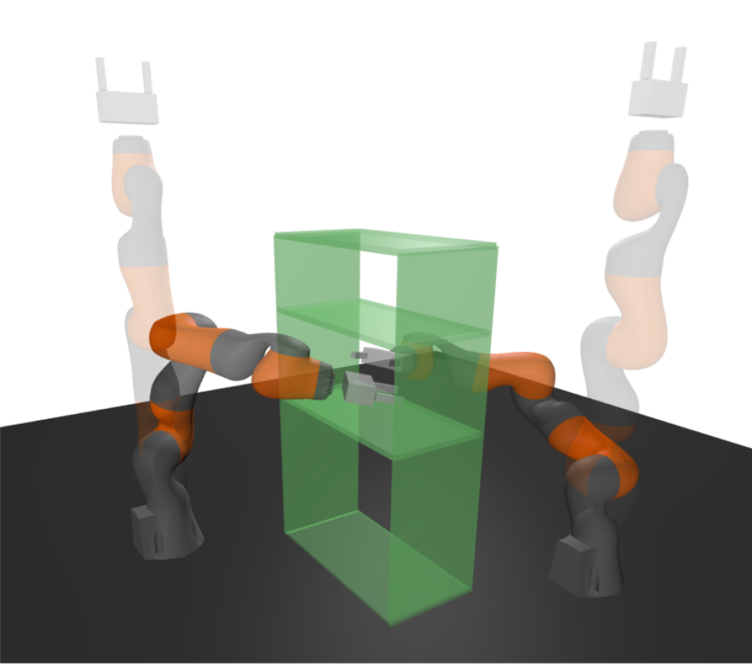
Figure 4: A pair of Kuka iiwa reaching from the straight up start configuration (translucent arms) into the shelf (opaque arms). The close confines of this motion plan make checking safety via finite sampling challenging. An animation of the motion plan is available here.

We consider the task of certifying a motion plan for a 12 degree of freedom (DOF) bimanual KUKA iiwa consisting of reaching into the shelf. The start and end configurations are shown in Figure 4. The environment contains 246 total collision pairs.

An RRT is grown in TC-space, with edges extended by sampling one hundred intermediate points between tree nodes. We grow the RRT until the task and goal are connected and the motion plan between them is certified as safe by (12). This requires 105 edges. Finally, we solve one instance of (12) for each collision pair and each edge for a total of 25830 programs with the hyperplane parameterized by a linear polynomial. All programs are solved in parallel.

In Figure 5(a), we plot the entire distribution of solve times for the 25830 programs. We group the collision geometry pairs by the highest degree condition given by (12). The most expensive program takes 297 ms to solve with Mosek [mosek], while the least expensive program takes 0.66 ms to solve. We note that Figure 5(a) is plotted on a log scale and demonstrates approximately quadratic growth as the degree of the polynomials increase to the right. On the other hand, almost no pattern is observed in the length of time taken to certify an individual edge for a given pair.

In Table I(a), we provide some aggregated statistics on the certification procedure. We recall that an edge of the RRT is considered safe if (12) is feasible for all 246 collision pairs. Due to the very close proximity of the collision geometries, we do not expect every edge to be collision-free. Indeed, we see that just under 30% of the edges in our tree are certified as collision free.

We observe that many of the uncertified edges correspond to motions in the tight confines of the shelf and so may in fact contain collisions. Therefore, if (12) for a given edge is not feasible for every collision pair, then we resample $1e5$, uniformly spaced configurations along that edge. If a collision is found, we confirm that the edge is NotSafe . Otherwise, we cannot confirm or deny the safety of the edge. We see that in 96% of cases, more dense sampling recovers a collision, which verifies that the infeasibility of (12) for these edges is not due to choosing too low a degree for the hyperplane. On the other hand, exactly two edges are neither declared safe , nor confirmed NotSafe . These two examples correspond to motions which undergo very large task space displacement of all links, but do not appear to contain collisions. It is likely the case that a higher degree polynomial could certify these edges.

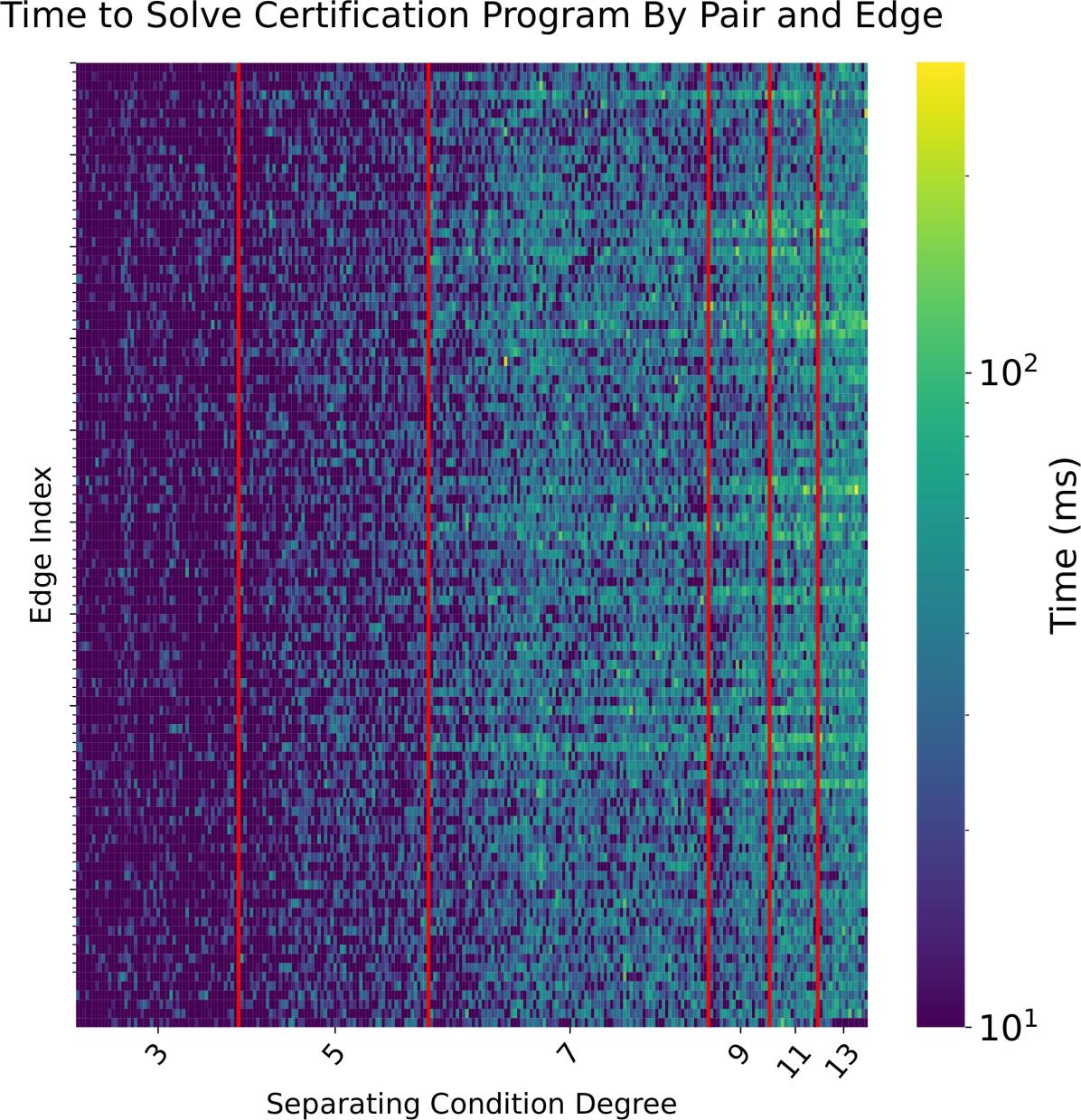
((a)) The time required to certify each edge and each collision pair in an RRT for the bimanual iiwa system. The y-axis is the index of the edge, and the x-axis is the index of the collision pair, grouped by the degree of the separating hyperplane condition (12b). The time taken to solve the certification program for a collision pair scales quadratically in the degree of the separating condition (12b)

Aggregate Statistics For Certifying the Entire RRT
# Instances of (12) Solved	25830
# Of Collision Pairs	246
# Of Edges	105
# Edges safe	31
# Edges Confirmed NotSafe	72
# Edges Unconfirmed NotSafe	2
Average Solver Time to Certify an Edge	299.9 msec.
Total Solver Time to Certify Goal Plan	1.211 sec.
Total Solver Time to Certify RRT	31.5 sec.

((a)) Aggregated statistics for certifying an RRT for the bimanual iiwa system. An edge is safe if all 246 instances of (12) are feasible. If (12) is infeasible, the corresponding edge is densely sampled with $1e5$ to find a collision. If a collision is found, the edge is confirmed NotSafe . We see that in two cases, neither (12) is feasible for all pairs, nor is a collision found. The final RRT plan is certified as safe in just over 1 second, and the whole tree is certified in about 30 seconds.

Figure 5: Timing statistics and aggregated statistics for certifying an RRT for the bimanual iiwa system from Figure 4. An instance of (12) is solved for all 246 collision pairs and all 105 edges in just over $30$ seconds.

V-B Certifying Cubic Polynomial Plans for a 7-DOF iiwa

We demonstrate our method’s ability to certify higher-order motion plans. We consider a 7-DOF Kuka iiwa interacting with a pair of shelves shown in Figure 1 moving along a piecewise polynomial plan with thirty pieces. Each piece is parametrized as a cubic, Hermite spline

We consider two such motion plans. The blue plan in Figure 1 is collision free, while exactly two of the thirty pieces of the red plan contain minor collisions with the shelf. We solve (12) with a linearly parametrized hyperplane for each segment of the plan.

In the case of the blue curve, all thirty pieces of motion plan are certified as safe in 8.99 seconds. Additionally, the twenty-eight pieces of the red plan which are safe are marked as safe . Meanwhile, the optimizer reported that (12) is infeasible for the two unsafe segments. The total time to solve the programs for unsafe plan was 9.21 seconds, which can be reduced to 6.91 seconds if the two unsafe segments are allowed to terminate as soon as one collision pair fails to certify its safety.

This demonstrates the precision of our method, which is capable of discriminating the safety of two visually indistinguishable motion plans.

VI Discussion and Conclusion

We present a method based on SOS programming for certifying non-collision along piecewise polynomial motion plans of arbitrary degree for kinematic systems composed of algebraic joints. These systems include the majority of open kinematic chain robots currently available. The proposed method provides fully rigorous certificates of non-colllision for individual linear motion plans in milliseconds even for high DOF systems and can certify more complicated plans in a handful of seconds.

Though currently not fast enough to fully replace a more rapid, sampling-based collision checker as a subroutine in a sampling-based motion planner, we anticipate that further efficiency improvements are possible. First, the number of instances of (12) can be dramatically reduced by pruning collision pairs which cannot possible collide on the motion plan using, for example, broad-phase collision checking [luque2005broad]. Secondly, all problems are solved using the general-purpose SDP solver Mosek. The formulation (12) has substantial structure for which accelerated solution methods exist [yuan2022polynomial].

The primary drawback to the adoption of our method is the requirement that the motion plans be algebraic, i.e. they must be given in a polynomial reparameterization of the configuration space such as the TC-space or the AC-space forcing the practioner to change their choice of configuration-space variable. In the case of standard randomized motion plans such as PRMs and RRTs, this can be as easy as simply changing the notion of distance and linear interpolation in the extend step of these methods.

While this may be a low barrier for purely kinematic motion plans, it may be more challenging for dynamic plans. The TC-space reparametrization greatly distorts configuration space near the joint angle $\theta_{i}=\pi$. Meanwhile the AC-space requires generating plans which conform to a strict constraint manifold.

Nevertheless, the proposed method is suitable for real world application, providing fully rigorous certificates of non-collision with provable correctness.

VII Acknowledgements

The authors are grateful to Hongkai Dai for his help in improving both the quality of this manuscript and the numerical implementation of this paper.

References

- [1] S. Cameron, “A study of the clash detection problem in robotics,” in Proceedings. 1985 IEEE International Conference on Robotics and Automation, vol. 2. IEEE, 1985, pp. 488–493.
- [2] L. He and J. van den Berg, “Efficient exact collision-checking of 3-d rigid body motions using linear transformations and distance computations in workspace,” in 2014 IEEE International Conference on Robotics and Automation (ICRA). IEEE, 2014, pp. 2059–2064.
- [3] M. Lin and S. Gottschalk, “Collision detection between geometric models: A survey,” in Proc. of IMA conference on mathematics of surfaces, vol. 1, 1998, pp. 602–608.
- [4] P. M. Hubbard, “Collision detection for interactive graphics applications,” IEEE Transactions on Visualization and Computer Graphics, vol. 1, no. 3, pp. 218–230, 1995.
- [5] M. I. Shamos and D. Hoey, “Geometric intersection problems,” in 17th Annual Symposium on Foundations of Computer Science (sfcs 1976). IEEE, 1976, pp. 208–215.
- [6] M. C. Lin, D. Manocha, and Y. J. Kim, “Collision and proximity queries,” in Handbook of discrete and computational geometry. Chapman and Hall/CRC, 2017, pp. 1029–1056.
- [7] J. Pan, S. Chitta, and D. Manocha, “Fcl: A general purpose library for collision and proximity queries,” in 2012 IEEE International Conference on Robotics and Automation. IEEE, 2012, pp. 3859–3866.
- [8] P. Jiménez, F. Thomas, and C. Torras, “3d collision detection: a survey,” Computers & Graphics, vol. 25, no. 2, pp. 269–285, 2001.
- [9] C. L. Jackins and S. L. Tanimoto, “Oct-trees and their use in representing three-dimensional objects,” Computer Graphics and Image Processing, vol. 14, no. 3, pp. 249–270, 1980.
- [10] F. Schwarzer, M. Saha, and J.-C. Latombe, “Exact collision checking of robot paths,” in Algorithmic foundations of robotics V. Springer, 2004, pp. 25–41.
- [11] X. Zhang, S. Redon, M. Lee, and Y. J. Kim, “Continuous collision detection for articulated models using taylor models and temporal culling,” ACM Transactions on Graphics (TOG), vol. 26, no. 3, pp. 15–es, 2007.
- [12] J. Canny, “Collision detection for moving polyhedra,” IEEE Transactions on Pattern Analysis and Machine Intelligence, no. 2, pp. 200–209, 1986.
- [13] A. Schweikard, “Polynomial time collision detection for manipulator paths specified by joint motions,” IEEE Transactions on robotics and automation, vol. 7, no. 6, pp. 865–870, 1991.
- [14] H. Dai, A. Amice, P. Werner, A. Zhang, and R. Tedrake, “Certified polyhedral decompositions of collision-free configuration space,” arXiv preprint arXiv:2302.12219, 2023.
- [15] S. Boyd, S. P. Boyd, and L. Vandenberghe, Convex optimization. Cambridge university press, 2004.
- [16] G. Blekherman, P. A. Parrilo, and R. R. Thomas, Semidefinite optimization and convex algebraic geometry. SIAM, 2012.
- [17] C. W. Wampler and A. J. Sommese, “Numerical algebraic geometry and algebraic kinematics,” Acta Numerica, vol. 20, 2011.
- [18] A. Amice, H. Dai, P. Werner, A. Zhang, and R. Tedrake, “Finding and optimizing certified, collision-free regions in configuration space for robot manipulators,” in Algorithmic Foundations of Robotics XV: Proceedings of the Fifteenth Workshop on the Algorithmic Foundations of Robotics. Springer, 2022, pp. 328–348.
- [19] P. A. Parrilo, Structured semidefinite programs and semialgebraic geometry methods in robustness and optimization. California Institute of Technology, 2000.
- [20] T. Roh and L. Vandenberghe, “Discrete transforms, semidefinite programming, and sum-of-squares representations of nonnegative polynomials,” SIAM Journal on Optimization, vol. 16, no. 4, pp. 939–964, 2006.
- [21] M.-D. Choi, T.-Y. Lam, and B. Reznick, “Real zeros of positive semidefinite forms. i,” Mathematische Zeitschrift, vol. 171, pp. 1–26, 1980.
- [22] R. Tedrake, Robotic Manipulation, 2021. [Online]. Available: https://manipulation.mit.edu/pick.html
- [23] M. Spivak, Calculus Third Edition. Cambridge University Press, 1994.
- [24] K. Mamou and F. Ghorbel, “A simple and efficient approach for 3d mesh approximate convex decomposition,” in 2009 16th IEEE international conference on image processing (ICIP). IEEE, 2009, pp. 3501–3504.
- [25] R. Tedrake and the Drake Development Team, “Drake: Model-based design and verification for robotics,” 2019. [Online]. Available: https://drake.mit.edu
- [26] M. ApS, The MOSEK optimization toolbox for MATLAB manual. Version 9.0., 2019. [Online]. Available: http://docs.mosek.com/9.0/toolbox/index.html
- [27] R. G. Luque, J. L. Comba, and C. M. Freitas, “Broad-phase collision detection using semi-adjusting bsp-trees,” in Proceedings of the 2005 symposium on Interactive 3D graphics and games, 2005, pp. 179–186.
- [28] C. Yuan, “Polynomial structure in semidefinite relaxations and non-convex formulations,” Ph.D. dissertation, Massachusetts Institute of Technology, 2022.