Pilot-Based Uplink Power Control in Single-UE Massive MIMO Systems With 1-Bit ADCs

Abstract

We propose uplink power control (PC) methods for massive multiple-input multiple-output systems with 1-bit analog-to-digital converters, which are specifically tailored to address the non-monotonic data detection performance with respect to the transmit power of the user equipment (UE) . Considering a single UE , we design a multi-amplitude pilot sequence to capture the aforementioned non-monotonicity, which is utilized at the base station to derive UE transmit power adjustments via single-shot or differential power control (DPC) techniques. Both methods enable closed-loop uplink PC using different feedback approaches. The single-shot method employs one-time multi-bit feedback, while the DPC method relies on continuous adjustments with 1-bit feedback. Numerical results demonstrate the superiority of the proposed schemes over conventional closed-loop uplink PC techniques.

Index Terms—1-bit ADCs, massive MIMO, uplink PC.

1 Introduction

Future wireless communication systems will push the carrier frequencies towards the (sub-)THz region to meet the demand for higher data rates and lower latency [1]. Beamforming with massive multiple-input multiple-output (MIMO) arrays can compensate for the increased pathloss at (sub-)THz frequencies, allowing for a cell radius comparable to that of sub-6 GHz systems. Fully digital massive MIMO architectures enable flexible beamforming and large-scale spatial multiplexing [2], although each antenna requires a dedicated radio-frequency chain. In this setting, the power consumption of the analog-to-digital converters (ADCs) scales linearly with the sampling rate and exponentially with the number of quantization bits [3, 4, 5, 6]. Consequently, low-resolution ADCs have been regarded as a promising enabler for high-frequency massive MIMO in recent years. In particular, 1-bit ADCs exhibit the lowest power consumption with a modest performance loss compared to unquantized systems. Several works have focused on the performance analysis of uplink massive MIMO systems with 1-bit ADCs , e.g., [3, 4, 7, 8, 9, 10]. Importantly, the performance of channel estimation and data detection with 1-bit ADCs is strongly affected by the operating signal-to-noise ratio (SNR) and, thus, by the transmit power of the user equipment (UE) [5, 9, 10].

Uplink power control (PC) is crucial for maintaining the signal-to-interference-plus-noise ratio (SINR) or the symbol error rate (SER) of each UE at the desired level, in addition to guaranteeing energy efficiency. In this regard, cellular networks require both open- and closed-loop uplink PC techniques. To this end, a framework for uplink PC is introduced in [11] while the uplink PC implementation of the Third-Generation Partnership Project (3GPP) Long-Term Evolution (LTE) standard is evaluated in [12]. When considering a conventional unquantized massive MIMO system, increasing the UE transmit power always leads to a monotonic improvement in the SER performance. However, this is not the case when 1-bit ADCs are involved due to distinct dominant degrading factors at low and high SNR , i.e., the additive white Gaussian noise (AWGN) and the 1-bit quantization distortion, respectively. Specifically, at high SNR , the 1-bit quantization distortion makes the soft-estimated symbols corresponding to transmit symbols with the same phase indistinguishable, leading to high SER [5, 9, 10]. Therefore, with 1-bit ADCs , the SER performance is no longer monotonic with the UE transmit power, and existing uplink PC techniques are not able to tackle this behavior.

In this paper, we fill this gap by proposing uplink PC methods for massive MIMO with 1-bit ADCs . Considering a single-UE scenario, our objective is to tune the UE transmit power to find the “right” operating SNR , i.e., where the data detection performance is not dominated by either the AWGN or the 1-bit quantization distortion. To this end, we introduce a multi-amplitude pilot sequence that is utilized at the base station (BS) to derive the UE transmit power adjustments. Then, we present two methods for calculating the UE transmit power adjustments using closed-loop uplink PC . In the first one, referred to as the single-shot method, the UE achieves a highly accurate transmit power level by means of a one-time multi-bit feedback from the BS . The second one, referred to as the differential power control (DPC) method, employs a continuous 1-bit feedback loop. The latter approach achieves substantial gains epecially in dynamic environments, despite the imprecise power adjustments compared with the single-shot method. Numerical results validate the superiority of the proposed methods compared to conventional approaches.

2 System Model

We consider a BS equipped with $M$ antennas serving a single UE equipped with a single antenna in the uplink. Each BS antenna is connected to two 1-bit ADCs for the in-phase and the quadrature components of the input signal. The received signal at the BS prior to the 1-bit ADCs is given by

$$\mathbf{Y}=\sqrt{\rho}\mathbf{h}\mathbf{x}^{\mathrm{H}}+\mathbf{Z}\in\mbox{$\mathbb{C}$}^{M\times N},\vspace{-1mm}$$ (1)

where $\rho$ is the UE transmit power, $\mathbf{h}\in\mbox{$\mathbb{C}$}^{M\times 1}$ is the uplink channel, $\mathbf{x}\in\mbox{$\mathbb{C}$}^{N\times 1}$ is the transmit symbol vector with $\mathbb{E}[\|\mathbf{x}\|^{2}]=N$, and $\mathbf{Z}\in\mbox{$\mathbb{C}$}^{M\times N}$ is the AWGN with entries distributed as $\mathcal{C}\mathcal{N}(0,1)$. As in [5, 9, 10], we assume that the channel is subject to i.i.d. Rayleigh fading, i.e., $\mathbf{h}\sim\mathcal{C}\mathcal{N}(0,\mathbf{I}_{M})$. However, the proposed framework applies to correlated channel models as well. Let us introduce the 1-bit quantization function $Q:\mbox{$\mathbb{C}$}\to\mathcal{Q}$, with ${Q(a)=\mathrm{sgn}\big{(}\mathrm{Re}[a]\big{)}+j\mathrm{sgn}\big{(}\mathrm{Im}[a]\big{)}}$ and $\mathcal{Q}=\{\pm 1\pm j\}$. At the output of the 1-bit ADCs, we have

$$\mathbf{R}=Q(\mathbf{Y})\in\mathcal{Q}^{M\times N}.\vspace{-1mm}$$ (2)

In the following, we briefly discuss the channel estimation and the data detection with 1-bit ADCs .

2.1 Channel Estimation and Data Detection

To estimate the channel, the UE transmits a pilot sequence $\mathbf{p}\in\mbox{$\mathbb{C}$}^{\tau\times 1}$ to the BS, with $\left\lVert\mathbf{p}\right\rVert^{2}=\tau$. Consequently, the received pilot signal at the BS prior to the 1-bit ADCs is given by

$$\mathbf{Y}_{\mathrm{p}(\rho)}=\sqrt{\rho}\mathbf{h}\mathbf{p}^{\mathrm{H}}+\mathbf{Z}_{\mathrm{p}}\in\mbox{$\mathbb{C}$}^{M\times\tau},\vspace{-1mm}$$ (3)

where $\mathbf{Z}_{\mathrm{p}}\in\mbox{$\mathbb{C}$}^{M\times\tau}$ is the AWGN with entries distributed as $\mathcal{C}\mathcal{N}(0,1)$. At the output of the 1-bit ADCs, we have

$$\mathbf{R}_{\mathrm{p}(\rho)}=Q(\mathbf{Y}_{\mathrm{p}})\in\mathcal{Q}^{M\times\tau}.\vspace{-1mm}$$ (4)

Then, the least-squares channel estimate (up to a scaling constant) is obtained by correlating $\mathbf{R}_{\mathrm{p}(\rho)}$ with the pilot vector, i.e.,

$$\hat{\mathbf{h}}=\mathbf{R}_{\mathrm{p}(\rho)}\mathbf{p}.\vspace{-1mm}$$ (5)

Upon estimating the channel, the BS obtains a soft estimate of the transmit symbol vector via linear combining as

$$\hat{\mathbf{x}}=\psi\mathbf{R}^{\mathrm{H}}\hat{\mathbf{h}}\in\mbox{$\mathbb{C}$}^{N\times 1},\vspace{-1mm}$$ (6)

where $\psi$ is a normalization factor such that $||\hat{\mathbf{x}}||^{2}=N$. Finally, the soft-estimated symbols in (6) are mapped to one of the transmit symbols, e.g., via minimum distance detection with respect to the expected values of the soft-estimated symbols [9, 10].

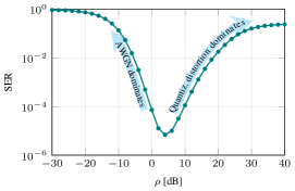
Fig. 1: SER versus UE transmit power.

2.2 Data Detection SER Analysis

Let $\{s_{1},\ldots,s_{\Lambda}\}$ and $\{\hat{s}_{1},\ldots,\hat{s}_{\Lambda}\}$ be the indices of the transmit symbols and of the detected symbols, respectively. Assuming that all the transmit symbols have equal probability, the SER is defined as

$$\lx@glossaries@gls@link{acronym}{ser}{\leavevmode\text{SER}}=\sum_{\lambda=1}^{\Lambda}\frac{1}{\Lambda}\mathbb{P}[s_{\lambda}\neq\hat{s}_{\lambda}|s_{\lambda}],\vspace{-1mm}$$ (7)

where $\Lambda$ denotes the order of the modulation scheme.

Fig. 1 illustrates the 16-quadrature amplitude modulation (QAM) SER with the UE transmit power for $M=256$. The SER is non-monotonic with respect to the UE transmit power due to the 1-bit quantization at the BS , unlike the unquantized system. Similar to the unquantized case, the SER is limited by the AWGN at the low SNR , and the SER improves with increasing the UE transmit power. However, after a certain UE transmit power, the SER starts to degrade due to the dominance of the quantization distortion, resulting in the aforementioned non-monotonicity.

3 Pilot-Based Uplink Power Control

In this section, we propose pilot-based uplink PC methods, a single-shot method, and a DPC method for massive MIMO systems with 1-bit ADCs , which are specifically tailored to address the non-monotonic data detection performance with respect to the UE transmit power. In this regard, we first introduce a multi-amplitude pilot sequence and derive the corresponding mean squared error (MSE) of the pilot estimation with 1-bit ADCs .

3.1 MSE of the Composite Pilot Estimation

The quantization distortion prevails in receiving the multi-amplitude input signal through the 1-bit ADCs . Therefore, we consider a pilot sequence with two amplitude levels which we call a composite pilot. Let ${\mathbf{q}=[\sqrt{\rho_{1}}\mathbf{p}^{\mathrm{T}},\sqrt{\rho_{2}}\mathbf{p}^{\mathrm{T}}]^{\mathrm{T}}\in\mbox{$\mathbb{C}$}^{2\tau\times 1}}$ be the composite pilot with power levels $\rho_{1}$ and ${\rho_{2}>\rho_{1}}$, where ${\mathbf{p}\in\mbox{$\mathbb{C}$}^{\tau\times 1}}$ consists of uni-modulus symbols. Given the transmitted signal $\mathbf{q}$, the received signal at the BS prior to quantization is

$$\mathbf{Y}_{\mathrm{q}} =[\mathbf{Y}_{\mathrm{p}(\rho_{1})},\mathbf{Y}_{\mathrm{p}(\rho_{2})}]$$

$$=[\sqrt{\rho_{1}}\mathbf{h}\mathbf{p}^{\mathrm{H}}+\mathbf{Z}_{\mathrm{p}(\rho_{1})},\sqrt{\rho_{2}}\mathbf{h}\mathbf{p}^{\mathrm{H}}+\mathbf{Z}_{\mathrm{p}(\rho_{2})}]\in\mbox{$\mathbb{C}$}^{M\times 2\tau}.\vspace{-1mm}$$ (8)

Note that the average power of $\mathbf{q}$ is ${(\rho_{1}+\rho_{2})/{2}}$ which we call composite pilot power. The received signal after quantization is

$$\mathbf{R}_{\mathrm{q}} =[\mathbf{R}_{\mathrm{p}(\rho_{1})},\mathbf{R}_{\mathrm{p}(\rho_{2})}]$$

$$=[Q(\mathbf{Y}_{\mathrm{p}(\rho_{1})}),Q(\mathbf{Y}_{\mathrm{p}(\rho_{2})})]\in\mathcal{Q}^{M\times 2\tau}.\vspace{-1mm}$$ (9)

From the quantized received pilot signal $\mathbf{R}_{\mathrm{q}}$, the channel can be estimated up to a scaling factor as in (5) (by replacing $\mathbf{p}$ with $\mathbf{q}$), and the average MSE of estimating the composite pilot can be computed as

$$\lx@glossaries@gls@link{acronym}{pilotmse}{\leavevmode\text{MSE}}\bigg{(}\frac{\rho_{1}+\rho_{2}}{2}\bigg{)} =\mathbb{E}\left[\left\lVert\frac{1}{\left\lVert\mathbf{R}_{\mathrm{q}}^{\mathrm{H}}\mathbf{R}_{\mathrm{q}}\mathbf{q}\right\rVert}\mathbf{R}_{\mathrm{q}}^{\mathrm{H}}\mathbf{R}_{\mathrm{q}}\mathbf{q}-\frac{1}{\left\lVert\mathbf{q}\right\rVert}\mathbf{q}\right\rVert^{2}\right].$$ (10)

which we call composite pilot estimation MSE or simply MSE , where the expectation is taken over the channel and the AWGN realizations depending on the availability.

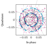
(a) $\rho=-30$ dB.

(b) $\rho=-2$ dB.

(c) $\rho=20$ dB.

Fig. 2: Impact of AWGN and quantization distortion on the received pilot symbols. $\circ$ - transmitted pilot symbols, $\times$ - received pilot symbols.

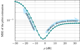
Fig. 3: MSE of the pilot estimation versus UE transmit power.

Fig. 3 shows the MSE versus the composite pilot power ${(\rho_{1}+\rho_{2})/{2}}$ with $M=256$ and ${\rho_{2}-\rho_{1}=5}$ dB. A Zadoff-Chu sequence with $\tau=127$ is used as $\mathbf{p}$. For the above scenario, the level of distortion for 3 interesting $\rho$ values is depicted in Fig. 2 on top of the page. Note that ${\rho_{2}-\rho_{1}=5}$ dB provides a quantization distortion similar to the 16-QAM SER as shown in Fig. 1. Therefore, we can use the MSE to optimize the SER performance over the UE transmit power. In the following, we discuss the proposed uplink PC methods that utilize the composite pilot estimation MSE .

3.2 Single-Shot Method

In open-loop PC , the UE estimates its pathloss using a downlink broadcast signal called synchronization signal block (SSB) . However, there is a $\rho_{\textnormal{\tiny{offset}}}$ error in the pathloss estimate. In the single-shot method, we estimate $\rho_{\textnormal{\tiny{offset}}}$ so that the UE transmit power to achieve the SER target can be obtained in a single pilot transmission. To this end, we consider a multi-amplitude pilot.

In general, for an odd number of amplitude levels $L$, the power of the amplitude level $\ell$ can be obtained (in dB) as

$$\rho_{\ell}=\lx@glossaries@gls@link{acronym}{rhostart}{\leavevmode\rho_{\mathrm{start}}}-\lx@glossaries@gls@link{acronym}{gap}{\leavevmode\Delta}+\frac{2(\ell-1)\lx@glossaries@gls@link{acronym}{gap}{\leavevmode\Delta}}{L-1}\quad[\mathrm{dB}],\quad\ell=1,\ldots,L,\vspace{-1mm}$$ (11)

where $\rho_{\mathrm{start}}$ (in dB) is a constant power shift and $\Delta$ (in dB) refers to the power gap. For example, considering $L=3$, $\lx@glossaries@gls@link{acronym}{rhostart}{\leavevmode\rho_{\mathrm{start}}}=0$ dB, and $\lx@glossaries@gls@link{acronym}{gap}{\leavevmode\Delta}=5$ dB, results in the transmitting power levels in $\{-5,0,5\}$ dB. Therefore we can estimate the MSE with composite pilot with $\{-5,0\}$ dB and $\{0,5\}$ dB UE transmit power levels, which correspond to the MSE at $\rho=-1.8170$ dB and $\rho=3.1830$ dB in Fig. 3, respectively. In this case, the overall span of the UE transmit power is $[-5,5]$ dB.

Let ${\mathbf{q}=\begin{bmatrix}\sqrt{\rho_{1}}\mathbf{p}^{\mathrm{T}}\ldots\sqrt{\rho_{L}}\mathbf{p}^{\mathrm{T}}\end{bmatrix}^{\mathrm{T}}\in\mbox{$\mathbb{C}$}^{L\tau}\times 1}$ be the transmit pilot sequence with $L$ amplitude levels. We call $\mathbf{q}$ a multi-amplitude pilot. The corresponding received signal after 1-bit quantization is

$$\mathbf{R}_{\mathrm{q}} =[\mathbf{R}_{\mathrm{p}(\rho_{1})},\ldots,\mathbf{R}_{\mathrm{p}(\rho_{L})}]$$ (12)

$$=[Q(\mathbf{Y}_{\mathrm{p}(\rho_{1})}),\ldots,Q(\mathbf{Y}_{\mathrm{p}(\rho_{L})})]$$

$$=[Q(\sqrt{\rho_{1}}\mathbf{h}\mathbf{p}^{\mathrm{H}}\!\!+\!\!\mathbf{Z}_{\mathrm{p}_{1}}),\ldots,Q(\sqrt{\rho_{L}}\mathbf{h}\mathbf{p}^{\mathrm{H}}\!\!+\!\!\mathbf{Z}_{\mathrm{p}_{L}})]\in\mathcal{Q}^{M\times L\tau}.\vspace{-1mm}$$

We consider any two amplitude level subsequences with a power difference of $\Delta$ out of $L$ subsequences in $\mathbf{q}$ to form the composite pilots. The MSE values are calculated with (10) having the composite pilot powers of $\lx@glossaries@gls@link{acronym}{compositepowervec}{\leavevmode\boldsymbol{{\rho}}^{\tiny\mathrm{comp}}}\in\mbox{$\mathbb{R}$}^{\frac{L+1}{2}\times 1}$ where $\rho^{\tiny\mathrm{comp}}_{i}=(\rho_{i}+\rho_{i+(L-1)/2})/2,i=1,\ldots,(L+1)/2$ (in linear scale). We compute the power offset $\rho_{\mathrm{offset}}$ as

$$\hat{\rho}_{\mathrm{offset}}=\underset{\rho_{\mathrm{offset}}}{\operatornamewithlimits{argmin}}\|\lx@glossaries@gls@link{acronym}{pilotmse}{\leavevmode\text{MSE}}^{\mathrm{ref}}(\lx@glossaries@gls@link{acronym}{compositepowervec}{\leavevmode\boldsymbol{{\rho}}^{\tiny\mathrm{comp}}}+\rho_{\mathrm{offset}})-\lx@glossaries@gls@link{acronym}{pilotmse}{\leavevmode\text{MSE}}^{\mathrm{est}}(\lx@glossaries@gls@link{acronym}{compositepowervec}{\leavevmode\boldsymbol{{\rho}}^{\tiny\mathrm{comp}}})\|^{2},\vspace{-1mm}$$ (13)

where $\lx@glossaries@gls@link{acronym}{pilotmse}{\leavevmode\text{MSE}}^{\mathrm{ref}}(\lx@glossaries@gls@link{acronym}{compositepowervec}{\leavevmode\boldsymbol{{\rho}}^{\tiny\mathrm{comp}}}+\rho_{\mathrm{offset}})$ is the vector consisting of the reference MSE values at the composite pilot powers $\lx@glossaries@gls@link{acronym}{compositepowervec}{\leavevmode\boldsymbol{{\rho}}^{\tiny\mathrm{comp}}}+\rho_{\mathrm{offset}}$ for the given setup, the mapping of which is stored at the BS . $\lx@glossaries@gls@link{acronym}{pilotmse}{\leavevmode\text{MSE}}^{\mathrm{est}}(\lx@glossaries@gls@link{acronym}{compositepowervec}{\leavevmode\boldsymbol{{\rho}}^{\tiny\mathrm{comp}}})$ is the vector consisting of the MSE estimated values having composite pilot powers of $\boldsymbol{{\rho}}^{\tiny\mathrm{comp}}$ . After computing the $\hat{\rho}_{\mathrm{offset}}$, the BS computes the suitable power level to achieve the SER target and feeds the power level back to the UE using a downlink control channel. This method is useful if the UE power is largely deviated from the desired value.

3.3 DPC Method

Although the DPC method is closed-loop, in contrast to the single-shot method, the BS and the UE maintain a constant feedback loop in order to keep a desired SER . In addition, the DPC method is designed with less pilot and feedback overhead compared to the single-shot method. In this method, the pilot consists of three amplitude levels having $\rho_{1}$, $\rho_{2}$, and $\rho_{3}$ power levels, such that ${\rho_{2}-\rho_{1}=\rho_{3}-\rho_{2}=\Delta}$ dB. Similar to the previous method, the BS estimates the MSE based on (10) with composite pilot powers of ${(\rho_{1}+\rho_{2})/2}$ and ${(\rho_{2}+\rho_{3})/2}$, respectively. Then, the BS computes the differential MSE as

$$\delta_{\lx@glossaries@gls@link{acronym}{pilotmse}{\leavevmode\text{MSE}}}=\lx@glossaries@gls@link{acronym}{pilotmse}{\leavevmode\text{MSE}}^{\text{est}}\bigg{(}\frac{\rho_{2}+\rho_{3}}{2}\bigg{)}-\lx@glossaries@gls@link{acronym}{pilotmse}{\leavevmode\text{MSE}}^{\text{est}}\bigg{(}\frac{\rho_{1}+\rho_{2}}{2}\bigg{)}.\vspace{-1mm}$$ (14)

If $\delta_{\lx@glossaries@gls@link{acronym}{pilotmse}{\leavevmode\text{MSE}}}>0$, the MSE is limited by the quantization distortion at the BS , or else by the AWGN . Given the $\delta_{\lx@glossaries@gls@link{acronym}{pilotmse}{\leavevmode\text{MSE}}}$ value, there exists a one-to-one map between the MSE and the SER . Subsequently, using the MSE to SER mapping, the BS feeds back the UE to increase its transmit power to meet the SER target if the target is not met and the SER is in the AWGN region similar to the unquantized system. However, increasing the UE transmit power to meet the SER in the quantization region leads to degradation in the SER . Therefore, the BS feeds back the UE to decrease its transmit power irrespective of the SER target if the SER is in the quantization distortion region. Thus the DPC method ensures that the UE operates in the AWGN -limited region at all times. Considering a 1-bit of feedback from the BS to the UE , the UE can only adjust the UE transmit power by the step size δρ dB.

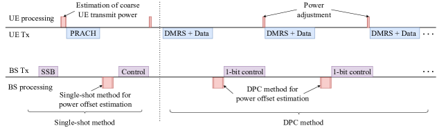
Fig. 4: Signaling and processing flow of the proposed 3GPP NR-based uplink PC implementation.

3.4 3GPP NR-Based Implementation

The proposed methods can be integrated with the 3GPP standard with minimal modifications, as shown in Fig. 4. Initially, the UE estimate the pathloss from the SSB and computes the coarse UE transmit power level to achieve the desired performance. Subsequently, the UE transmits Zadoff-Chu pilot sequences with $L$ amplitude levels in the physical random access channel (PRACH) repeatedly with stepwise increase of $\rho_{\mathrm{start}}$ value until a random-access response (RAR) is received from the BS . This is in contrast to the current standard where a PRACH contains only a single amplitude. In Fig. 4, the BS happens to detect the PRACH in just one transmission. This allows the BS to find the desired power level of the UE using the single-shot method as discussed in Section 3.2. After computing the desired UE transmit power level, the BS can give feedback on the power level using a control signal. However, in the connected mode, if the desired power deviation is small due to shadow or large-scale fading, the single-shot method may not be optimal due to resource overhead. Therefore, the DPC method can be utilized to control the small deviations in the power level. In this, the UE transmits demodulation reference signal (DMRS) (DMRS) pilot with three amplitude levels along with the data. Then, the BS computes the increment or decrement of the UE transmit power in steps of $\delta\rho$ based on the SER requirement as discussed in Section 3.3. Then, the BS provides a 1-bit of feedback to the UE using the control signal. Subsequently, the UE adjusts its power by $\pm\lx@glossaries@gls@link{acronym}{stepsize}{\leavevmode\delta\rho}$ in the next transmission.

4 Numerical Results

We consider $M=256$ BS antennas. The power difference in the composite pilot is $\Delta=5$ dB. The MSE and SER reference tables against the UE transmit power are generated with $10^{6}$ Monte-Carlo iterations for each of the simulated $(M,\tau,\lx@glossaries@gls@link{acronym}{gap}{\leavevmode\Delta})$ combination and are stored at the BS . Finally, there exists a one-to-one map of MSE to SER based on the AWGN -dominant region and the quantization-distortion-dominant region.

To evaluate the performance of the single-shot method, we assume that the power offset at the UE , i.e., $\rho_{\textnormal{\tiny{offset}}}$ , is uniformly distributed in $[-5,5]$ dB. Then, the UE transmits the pilot with $L$ amplitude levels and the length of each uni-modulus signal is $\tau$. The overall span of the UE transmit power levels is $10$ dB, and the power of each level is chosen as in (11) where $\lx@glossaries@gls@link{acronym}{rhostart}{\leavevmode\rho_{\mathrm{start}}}=0$ dB. Fig. 5 shows the average squared error in the power offset estimation for different values of $L$ and $\tau$. When $\tau$ is constant, the average squared error in the power offset estimation decreases as $L$ increases. For a given $L$, increasing $\tau$ always gives better performance. When the pilot overhead, i.e., $L\tau$, is constant, the performance degrades as we increase $L$, suggesting that $\tau$ has a stronger impact on the performance compared to $L$.

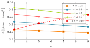
Fig. 5: $\mathbb{E}\left[|\hat{\rho}_{\text{\tiny offset}}-\rho_{\text{\tiny offset}}|^{2}\right]$ versus $L$.

To evaluate the performance of the DPC method, we consider $\lx@glossaries@gls@link{acronym}{stepsize}{\leavevmode\delta\rho}=0.5$ dB, $L=3$, $\tau=7$, $\lx@glossaries@gls@link{acronym}{rhostart}{\leavevmode\rho_{\mathrm{start}}}=0$ dB, and a shadowing environment as described in [13, Ch. 2], with an SER target of ${5\times 10^{-5}}$. The pathloss model is ${-61-30\log_{10}(d)}$ dB where $d$ is the distance from the BS to the UE in meters. At ${t=0}$, the distance between the UE and the BS is approximately ${63.73}$ m, considering a pathloss compensation with an offset of ${\lx@glossaries@gls@link{acronym}{plesterr}{\leavevmode\rho_{\textnormal{\tiny{offset}}}}=-5}$ dB based on the SSB . The UE moves $50$ m with a constant velocity of $20$ m/s towards the BS subject to shadowing. The PC feedback rate is $100$ bps. The performance of the proposed DPC method is compared with the conventional PC method, where the UE transmit power is increased if the target SER is not met or else it is decreased by $\delta\rho$ . Also, we compare with the fixed power, i.e., UE transmits with a fixed power irrespective of the SER target. In Fig. 6, the 16-QAM SER is plotted over time, where the shadow and large-scale changes with time. The SER target is met with the proposed DPC method with a reasonable level of fluctuation. However, using the conventional PC method may degrade the SER if the BS is in the quantization distortion region. Eventually, it can perform worst than the fixed power case. The SER of the fixed power case changes with the shadow and large-scale fading. Hence, the proposed DPC method is robust against shadow and large-scale fading.

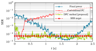
Fig. 6: SER versus time for the proposed closed-loop uplink PC strategies.

5 Conclusions

This paper explores the uplink PC of single-UE MIMO systems with 1-bit ADCs . The presence of non-monotonic behavior in MSE or SER with respect to the UE transmit power with 1-bit ADCs renders the standard uplink PC approach less effective in optimizing UE transmit powers for improved performance. To address this challenge, we propose a novel approach that leverages a multi-amplitude pilot received at the BS to tune the UE transmit power using the single-shot and the DPC methods. The single-shot method determines the desired power level of the UE , using only one pilot transmission stage. Next, we introduce the DPC method, where the UE transmit power is adjusted incrementally with a fixed step size, guided by the SER behavior mapped from the MSE of the received pilot signals at the BS . To evaluate the effectiveness of the proposed algorithm, we conducted experiments in an environment with shadow fading. The results demonstrate the superiority of the proposed methods over standard approaches. Future work will consider extensions to multi-UE settings involving more realistic channel models.

References

- [1] N. Rajatheva, I. Atzeni, E. Björnson et al., “White paper on broadband connectivity in 6G,” 2020, White Paper.
- [2] T. L. Marzetta, “Noncooperative cellular wireless with unlimited numbers of base station antennas,” IEEE Trans. Wireless Commun., vol. 9, no. 11, pp. 3590–3600, 2010.
- [3] J. Mo and R. W. Heath, “Capacity analysis of one-bit quantized MIMO systems with transmitter channel state information,” IEEE Trans. Signal Process., vol. 63, no. 20, pp. 5498–5512, 2015.
- [4] Y. Li, C. Tao, G. Seco-Granados, A. Mezghani, A. L. Swindlehurst, and L. Liu, “Channel estimation and performance analysis of one-bit massive MIMO systems,” IEEE Trans. Signal Process., vol. 65, no. 15, pp. 4075–4089, 2017.
- [5] S. Jacobsson, G. Durisi, M. Coldrey, U. Gustavsson, and C. Studer, “Throughput analysis of massive MIMO uplink with low-resolution ADCs,” IEEE Trans. Wireless Commun., vol. 16, no. 6, pp. 1304–1309, 2017.
- [6] I. Atzeni, A. Tölli, and G. Durisi, “Low-resolution massive MIMO under hardware power consumption constraints,” in Proc. Asilomar Conf. Signals, Syst., and Comput. (ASILOMAR), 2021.
- [7] C. Mollén, J. Choi, E. G. Larsson, and R. W. Heath, “Uplink performance of wideband massive MIMO with one-bit ADCs,” IEEE Trans. Wireless Commun., vol. 16, no. 1, pp. 87–100, 2017.
- [8] A. B. Üçüncü and A. Ö. Yılmaz, “Oversampling in one-bit quantized massive MIMO systems and performance analysis,” IEEE Trans. Wireless Commun., vol. 17, no. 12, pp. 7952–7964, 2018.
- [9] I. Atzeni and A. Tölli, “Channel estimation and data detection analysis of massive MIMO with 1-bit ADCs,” IEEE Trans. Wireless Commun., vol. 21, no. 6, pp. 3850–3867, 2022.
- [10] ——, “Uplink data detection analysis of 1-bit quantized massive MIMO,” in Proc. IEEE Int. Workshop Signal Process. Adv. in Wireless Commun. (SPAWC), 2021.
- [11] R. D. Yates, “A framework for uplink power control in cellular radio systems,” IEEE J. Sel. Areas Commun., vol. 13, no. 7, pp. 1341–1347, 1995.
- [12] A. Simonsson and A. Furuskar, “Uplink power control in LTE – overview and performance,” in Proc. IEEE Veh. Technol. Conf. (VTC), 2008.
- [13] D. Tse and P. Viswanath, Fundamentals of Wireless Communication, 1st ed. Cambridge University Press, 2005.