Intense anomalous high harmonics in graphene quantum dots caused by disorder or vacancies

Abstract

This article aims to study the linear and nonlinear optical response of inversion symmetric graphene quantum dots (GQDs) in the presence of on-site disorder or vacancies. The presence of disorder or vacancy breaks the special inversion symmetry leading to the emergence of intense Hall-type anomalous harmonics. This phenomenon is attributed to the intrinsic time-reversal symmetry-breaking in quantum dots with a pseudo-relativistic Hamiltonian, even in the absence of an external magnetic field. We demonstrate that the effects induced by disorder or vacancy have a distinct impact on the optical response of GQDs. In the linear response, we observe significant Hall conductivity. In the presence of an intense laser field, we observe the radiation of strong anomalous odd and even-order harmonics already for relatively small levels of disorder or mono-vacancy. The both disorder and vacancy lift the degeneracy of states, thereby creating new channels for interband transitions and enhancing the emission of near-cutoff high-harmonic signals.

I Introduction

Theoretical studies of two-dimensional (2D) systems with unique electronic and topological properties can be traced back about 80 years, encompassing areas such as single graphite layers [1, 2], zero-gap semiconductors [3], the quantum Hall effect without a magnetic field [4], d-wave superconductors [5], and neutrino billiards [6]. However, it was only with the experimental realization of graphene in 2004 [7] that a new frontier in physics opened up: the field of 2D materials featuring pseudo-relativistic charged carriers and nontrivial spatial and band structure topology [8, 9, 10, 11, 12]. One remarkable manifestation of the importance of topology is the ”mystery of a missing pie” [13] in the DC conductivity of graphene $\sigma_{DC}$. Early experiments observed values of $\sigma_{DC}$ that were $\pi$ times larger than the predicted value for pristine, disorder-free graphene [14]. Subsequent studies revealed that the value of $\sigma_{DC}$ strongly depends on various factors, including the boundary conditions of the graphene sheet [15, 16], the presence of disorder[17, 18], and the interactions among charged carriers [19, 20, 21]. This highlighted the intricate interplay between topology, disorder, and carrier interactions in graphene’s electrical conductivity.

The optoelectronic properties of graphene undergo significant changes when it is reduced to zero-dimensional structures known as graphene quantum dots (GQDs) [22]. The behavior of GQDs can vary from metallic to insulating, depending on the type of edges they possess [23]. The optical properties of GQDs depend on their size and shape [24, 25, 22, 26, 27].

Various synthesis methods exist for GQDs, including fragmentation of fullerene molecules [28] and nanoscale cutting of graphite combined with exfoliation [29], decomposition of hydrocarbons [30]. The confinement of electronic states in GQDs has been confirmed through scanning tunneling microscopy measurements [31]. Along with graphene, GQDs have garnered significant attention due to their unique optoelectronic properties and their potential applications in diverse fields such as bioimaging [32, 33], photovoltaics [34], quantum computing [35], photodetectors [36], energy storage [37], sensing [38], and metal ion detection [39].

The potential to engineer the energy spectrum and optical transitions of GQDs has got significant attention also in the field of strong-field physics [40]. This is due to the promising prospects for GQDs in extreme nonlinear optics applications, including high-order harmonic generation (HHG) [41]. Theoretical studies have predicted strong HHG from fullerenes [42, 43, 44, 45, 46], graphene nanoribbons [47, 48, 49], and GQDs [50, 51, 52, 53, 54]. These studies have also highlighted significant alterations in the nonlinear optical properties by manipulating the size, shape, and edges of these systems. It is worth noting that the electron-electron interactions have been recognized as a crucial factor that influence on the optical phenomena in the mentioned nanostructures [54].

In most previous theoretical studies, the interaction of graphene-like systems with the laser fields has been primarily focused on perfect crystal structures with periodic lattices. However, as is known disorder or point defects in graphene, such as vacancies can strongly affect the electronic properties of the system, since those defects support quasi-localized electronic states [55, 56, 57]. Recent studies have demonstrated that an imperfect lattice can lead to enhancement of HHG compared to a perfect lattice, particularly when considering doping-type impurities or disorder [58, 59, 60, 61, 46]. This raises the question of how the disorder or vacancies specifically affect the HHG spectra in GQDs. It is worth noting that GQDs with sharp boundaries exhibit time-reversal symmetry-breaking even in the absence of a magnetic field [6], suggesting the possibility of Hall-type anomalous responses in both linear and nonlinear regimes for imperfect GQDs. In this study, we present a microscopic theory that explores the linear and nonlinear interaction of GQDs with strong coherent electromagnetic radiation in the presence of on-site disorder or vacancy. Specifically, we investigate hexagonal GQD with a moderate size, as illustrated in Figure 1. By employing up to 10th nearest-neighbor hopping integrals within a dynamical Hartree-Fock (HF) approximation, we reveal the polarization-resolved structure of the HHG spectrum.

The paper is organized as follows. In Sec. II, the model with the basic equations are formulated. In Sec. III the linear optical response is considered. In Sec. IV, we present the results regarding nonlinear optical response. Finally, conclusions are given in Sec. V.

II The model

The basic GQD₂₁₆, illustrated in Fig. 1, has symmetry described by the non-abelian point group C_6v. We also consider GQD₂₁₆ with on-site disorder and GQD₂₁₆ with a mono-vacancy. GQD is assumed to interact with a laser pulse that excites electron coherent dynamics. We assume a neutral GQD that will be described in the scope of the TB theory. Hence, the total Hamiltonian reads:

$$\widehat{H}=\widehat{H}_{\mathrm{TB}}+\widehat{H}_{\mathrm{C}}+\widehat{H}_{\mathrm{int}},$$ (1)

where

$$\widehat{H}_{\mathrm{TB}}=\sum_{i\sigma}\varepsilon_{i}c_{i\sigma}^{\dagger}c_{j\sigma}-\sum_{i,j\sigma}t_{ij}c_{i\sigma}^{\dagger}c_{j\sigma}$$ (2)

is the free GQD TB Hamiltonian. Here $c_{i\sigma}^{\dagger}$ ($c_{i\sigma}$) creates (annihilates) an electron with the spin polarization $\sigma=\left\{\uparrow,\downarrow\right\}$ at the site $i$ ($\overline{\sigma}$ is the opposite to $\sigma$ spin polarization). In Eq. (2) $\varepsilon_{i}$ is the energy level at the site $i$, and $t_{ij}$ is the hopping integral between the sites $i$ and $j$.

The second term in the total Hamiltonian (1) describes the electron-electron interaction (EEI):

$$\widehat{H}_{\mathrm{C}}=\frac{U}{2}\sum_{i\sigma}c_{i\sigma}^{\dagger}c_{i\sigma}c_{i\overline{\sigma}}^{\dagger}c_{i\overline{\sigma}}+\frac{1}{2}\sum_{i,j\sigma\sigma^{\prime}}V_{ij}c_{i\sigma}^{\dagger}c_{i\sigma}c_{j\sigma^{\prime}}^{\dagger}c_{j\sigma^{\prime}},$$ (3)

with the parameters $U$ and $V_{ij}$ representing the on-site, and the long-range Coulomb interactions, respectively. The last term in the total Hamiltonian (1) is the light-matter interaction part that is described in the length-gauge:

$$\widehat{H}_{\mathrm{int}}=e\sum_{i\sigma}\mathbf{r}_{i}\cdot\mathbf{E}\left(t\right)c_{i\sigma}^{\dagger}c_{i\sigma},$$ (4)

with the elementary charge $e$, position vector $\mathbf{r}_{i}$, and the electric field strength $\mathbf{E}\left(t\right)$.

In this work, EEI is treated in the HF mean-field approximation employing the correlation expansion

$$\left\langle c_{1}^{\dagger}c_{2}^{\dagger}c_{3}c_{4}\right\rangle=\left\langle c_{1}^{\dagger}c_{4}\right\rangle\left\langle c_{2}^{\dagger}c_{3}\right\rangle-\left\langle c_{1}^{\dagger}c_{3}\right\rangle\left\langle c_{2}^{\dagger}c_{4}\right\rangle.$$

This factorization technique allows us to obtain a closed set of equations for the single-particle density matrix $\rho_{ji}^{\left(\sigma\right)}=\left\langle c_{i\sigma}^{\dagger}c_{j\sigma}\right\rangle$. We will assume that in the static limit the EEI Hamiltonian vanishes $\widehat{H}_{\mathrm{C}}^{HF}\simeq 0$. That is, EEI in the HF limit is included non-explicitly in empirical TB parameters $\widetilde{\varepsilon}_{i}$, $\widetilde{t}_{ij}$ which is chosen to be close to experimental values. For this propose in this paper we use up to 10th nearest-neighbor hopping $\widetilde{t}_{ij}$ with values taken from density functional theory by Wannierization [62] (see Table 1). Hence, the Hamiltonian $\widehat{H}_{\mathrm{TB}}+\widehat{H}_{\mathrm{C}}$ is approximated by,

$$\widehat{H}_{0}^{HF}=\sum_{i\sigma}\widetilde{\varepsilon}_{i}c_{i\sigma}^{\dagger}c_{j\sigma}-\sum_{i,j\sigma}\widetilde{t}_{ij}c_{i\sigma}^{\dagger}c_{j\sigma}+U\sum_{i}\left(\overline{n}_{i\uparrow}-\overline{n}_{0i\uparrow}\right)n_{i\downarrow}$$

$$+U\sum_{i\sigma}\left(\overline{n}_{i\downarrow}-\overline{n}_{0i\downarrow}\right)n_{i\uparrow}+\sum_{\left\langle i,j\right\rangle}V_{ij}\left(\overline{n}_{j}-\overline{n}_{0j}\right)n_{i}$$

$$-\sum_{i,j\sigma}V_{ij}c_{i\sigma}^{\dagger}c_{j\sigma}\left(\left\langle c_{i\sigma}^{\dagger}c_{j\sigma}\right\rangle-\left\langle c_{i\sigma}^{\dagger}c_{j\sigma}\right\rangle_{0}\right),$$ (5)

where $\overline{n}_{i\sigma}=\left\langle c_{i\sigma}^{\dagger}c_{i\sigma}\right\rangle=\rho_{ii}^{\left(\sigma\right)}$. In this representation the initial density matrix $\rho_{ji}^{\left(\sigma\right)}\left(0\right)=\left\langle c_{i\sigma}^{\dagger}c_{j\sigma}\right\rangle_{0}$ is calculated with respect to renormalized tight-binding Hamiltonian $\widehat{H}_{0}^{t}=-\sum_{i,j\sigma}\widetilde{t}_{ij}c_{i\sigma}^{\dagger}c_{j\sigma}$. From the Heisenberg equation we obtain evolutionary equations for the single-particle density matrix $\rho_{ij}^{\left(\sigma\right)}=\left\langle c_{j\sigma}^{\dagger}c_{i\sigma}\right\rangle$:

$$i\hbar\frac{\partial\rho_{ij}^{\left(\sigma\right)}}{\partial t}=\sum_{k}\left(\tau_{kj\sigma}\rho_{ik}^{\left(\sigma\right)}-\tau_{ik\sigma}\rho_{kj}^{\left(\sigma\right)}\right)+\left(V_{i\sigma}-V_{j\sigma}\right)\rho_{ij}^{\left(\sigma\right)}$$

$$+e\mathbf{E}\left(t\right)\left(\mathbf{r}_{i}-\mathbf{r}_{j}\right)\rho_{ij}^{\left(\sigma\right)}-i\hbar\gamma\left(\rho_{ij}^{\left(\sigma\right)}-\rho_{0ij}^{\left(\sigma\right)}\right),$$ (6)

where

$$V_{i\sigma}=\sum_{j\alpha}V_{ij}\left(\rho_{jj}^{\left(\alpha\right)}-\rho_{0jj}^{\left(\alpha\right)}\right)+U\left(\rho_{ii}^{\left(\overline{\sigma}\right)}-\rho_{0ii}^{\left(\overline{\sigma}\right)}\right),$$ (7)

and

$$\tau_{ij\sigma}=-\widetilde{\varepsilon}_{i}\delta_{ij}+\widetilde{t}_{ij}+V_{ij}\left(\rho_{ji}^{\left(\sigma\right)}-\rho_{0ji}^{\left(\sigma\right)}\right).$$ (8)

Electron-electron, electron-phonon scattering processes have been introduced in Eq. (6) phenomenologically via damping term, assuming that the system relaxes at a rate $\gamma$ to the equilibrium $\rho_{0ij}^{\left(\sigma\right)}$ distribution.

Table 1: The first row represents $n$th-nearest-neighbor order. The second row is the set of tight-binding parameters, where $t_{ii}=\widetilde{\epsilon}_{0}$. The third row is the Coulomb interaction matrix elements. The first three elements, where $U=V_{ii},$ are obtained from numerical calculations by using Slater $\pi_{z}$ orbitals [63, 22]. The longer range Coulomb interaction is taken to be ${\epsilon}_{d}V_{ij}=14.4/d_{ij}$ $eV$, where $d_{ij}$ is the distance in angstrom between the distant neighbors. Here ${\epsilon}_{d}$ is an effective dielectric constant which accounts for the substrate-induced screening in the 2D nanostructure.

nearest-neighbor	$0$	$1$	$2$	$3$	$4$	$5$	$6$	$7$	$8$	$9$	$10$
$t_{ij}\ [\mathrm{eV}]$	$0.297$	$2.912$	$-0.223$	$0.289$	$-0.025$	$-0.055$	$0.022$	$0.013$	$0.022$	$-0.007$	$-0.004$
${\epsilon}_{d}V_{ij}\ [\mathrm{eV}]$	$16.5$	$8.6$	$5.3$	$14.4/d_{i3}$	$14.4/d_{i4}$	$14.4/d_{i5}$	$14.4/d_{i6}$	$14.4/d_{i7}$	$14.4/d_{i8}$	$14.4/d_{i9}$	$14.4/d_{i10}$

In the present paper, as a first approximation, mono-vacancy is simulated by setting the hopping parameters to the empty site to zero and the on-site energy at the empty site equals to a large value outside the energy range of the density of states [64]. There is also scenario when the structure undergoes a bond reconstruction in the vicinity of the vacancy [65]. In either case, a local distortion of the lattice takes place resulting states that are strongly localized around defects [66, 67]. In the tight-binding Hamiltonian (5) the diagonal disorder is described by the Anderson model introducing randomly distributed site energies $\epsilon_{ri}$: $\widetilde{\epsilon}_{i}=\widetilde{\epsilon}_{0i}+\epsilon_{ri}$. We assume for the random variable $\epsilon_{ri}$ to have probability distributions $P\left(\epsilon_{ri},V_{\mathrm{on}}\right)$, where

$$P\left(\epsilon_{ri},V_{\mathrm{on}}\right)=\left\{\begin{array}[]{c}\frac{1}{2V_{\mathrm{on}}},\ -V_{\mathrm{on}}\leq\epsilon_{ri}\leq V_{\mathrm{on}}\\ 0,\ \mathrm{otherwise}\end{array}\right..$$ (9)

Here the quantity $V_{\mathrm{on}}$ is the distribution width describing the strength of the disorder. The disorder strength for all calculations is taken to be $V_{\mathrm{on}}$=0.3 eV.

III Linear optical response

The linear optical response of the considered system is completely described by the initial equilibrium $\rho_{0ij}^{\left(\sigma\right)}$ distribution function. For this propose we need the eigenfunctions ($\psi_{\sigma\mu}\left(i\right)$) and eigenenergies ($\varepsilon_{\sigma\mu}$) of the TB Hamiltonian. We numerically diagonalize the TB Hamiltonian with the parameters from Table 1, and construct the initial density matrix $\rho_{0ij}^{\left(\sigma\right)}$ via the filling of electron states in the valence band according to the zero temperature Fermi–Dirac-distribution $\rho_{0ij}^{\left(\sigma\right)}=\sum_{\mu=N/2}^{N-1}\psi_{\sigma\mu}^{\ast}\left(j\right)\psi_{\sigma\mu}\left(i\right)$. In Fig. 1 the electron probability density $\left|\psi_{\sigma\mu}\left(i\right)\right|^{2}$ on the 2D color mapped nanostructure corresponding to the highest energy level in the valence band and eigenenergies near the Fermi level are shown. In both cases we see the emergence of states near the Fermi level. As is also seen from this figure, the presence of on-site disorder or a mono-vacancy breaks the inversion symmetry. As expected, in the case of a vacancy we have a state that is strongly localized around the defect. To provide a quantitative characterization of localization in the $\mu$-th eigenstates, we also calculate the inverse participation number

$$P_{\mu}=\left(\sum_{i=0}^{N-1}\left|\psi_{\mu}\left(i\right)\right|^{4}\right)^{-1},$$ (10)

which provides a measure of the fraction of sites over which the wavepacket is spread [68]. The normalized inverse participation numbers $P_{\mu}/N$ for states near the Fermi level are illustrated in Fig. 2. From this figure it becomes evident that these states are localized, which as we will see, strongly alter the optical response of the considered nanostructures. For the higher energy states $P_{\mu}/N\sim 0.5$, which means that those states are more resistant to defects.

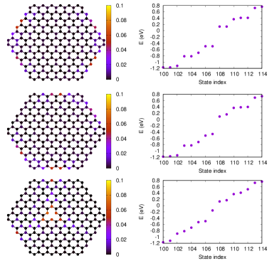
Figure 1: The top row represents intrinsic GQD₂₁₆, the middle row depicts GQD₂₁₆ with disorder, and the bottom row illustrates GQD₂₁₆ with a monovacancy. Within each row, the following visualizations are presented from left to right: electron probability density corresponding to the highest energy level in the valence band and eigenenergies near the Fermi level.

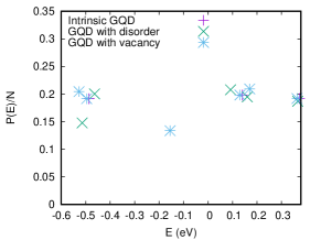
Figure 2: The normalized inverse participation number for states near the Fermi level.

To study the linear response we first need to calculate the susceptibility tensor $\chi_{ij}$ which is more transparent to give in the energetic representation. For this propose we perform a basis transformation using the following formula:

$$\rho_{ij}^{(\sigma)}=\sum_{\mu^{\prime}}\sum_{\mu}\psi_{\sigma\mu^{\prime}}^{\ast}\left(j\right)\varrho_{\sigma\mu\mu^{\prime}}\psi_{\sigma\mu}\left(i\right),$$ (11)

where $\varrho_{\sigma\mu\mu^{\prime}}$ is the density matrix in the energetic representation. Taking into account the completeness of basis functions, from Eq. (6) we get the following equation

$$i\hbar\frac{\partial\varrho_{\sigma mn}}{\partial t}=\left(\varepsilon_{\sigma m}-\varepsilon_{\sigma n}\right)\varrho_{\sigma mn}$$

$$+\mathbf{E}\left(t\right)\sum_{\mu}\left(\varrho_{\sigma\mu n}\mathbf{d}_{\sigma m\mu}-\varrho_{\sigma m\mu}\mathbf{d}_{\sigma\mu n}\right)-i\hbar\gamma\left(\varrho_{\sigma mn}-\varrho_{\sigma mn}^{(0)}\right),$$ (12)

where $\mathbf{d}_{\sigma\mu^{\prime}\mu}=e\sum_{i}\psi_{\sigma\mu^{\prime}}^{\ast}\left(i\right)\mathbf{r}_{i}\psi_{\sigma\mu}\left(i\right)$ is the transition dipole moment. We will solve Eq. (12) in the scope of perturbation theory by expanding the density matrix in orders of the incident electromagnetic field

$$\varrho_{\sigma mn}=\varrho_{\sigma mn}^{(0)}+\varrho_{\sigma mn}^{(1)}.$$ (13)

Assuming $E_{j}\left(t\right)=\sum_{\omega}E_{j}\left(\omega\right)e^{-i\omega t}$, it is straightforward to obtain

$$\varrho_{\sigma mn}^{(1)}=\sum_{j\omega}\frac{E_{j}\left(\omega\right)e^{-i\omega t}d_{\sigma mn}^{j}\left(\varrho_{\sigma nn}^{(0)}-\varrho_{\sigma mm}^{(0)}\right)}{\varepsilon_{\sigma m}-\varepsilon_{\sigma n}-\hbar\omega-i\hbar\gamma}.$$

The polarization vector $P_{i}\left(t\right)=\sum_{\sigma mn}\varrho_{\sigma mn}^{(1)}\left(t\right)d_{\sigma nm}^{i}$ now can be expressed as:

$$P_{i}\left(t\right)=\sum_{\sigma mn}\sum_{j\omega}\frac{E_{j}\left(\omega\right)e^{-i\omega t}d_{\sigma mn}^{j}\left(\varrho_{\sigma nn}^{(0)}-\varrho_{\sigma mm}^{(0)}\right)}{\varepsilon_{\sigma m}-\varepsilon_{\sigma n}-\hbar\omega-i\hbar\gamma}.$$ (14)

Taking into account the definition $P_{i}=\epsilon_{0}\sum_{j}\chi_{ij}E_{j}$, where $\epsilon_{0}$ is the electric permittivity of free space, from Eq. (14) we get:

$$\chi_{ij}\left(\omega\right)=\frac{1}{\epsilon_{0}}\sum_{\sigma mn}\varrho_{\sigma mm}^{(0)}\left[\frac{d_{\sigma nm}^{j}d_{\sigma mn}^{i}}{\varepsilon_{\sigma n}-\varepsilon_{\sigma m}-\hbar\omega-i\hbar\gamma}\right.$$

$$\left.+\frac{d_{\sigma mn}^{j}d_{\sigma nm}^{i}}{\varepsilon_{\sigma n}-\varepsilon_{\sigma m}+\hbar\omega+i\hbar\gamma}\right].$$ (15)

With the help of susceptibility tensors in SI units we also calculate the conductivity tensors in CGS units by the formula

$$\sigma_{ij}\left(\omega\right)=-i\epsilon_{0}\omega\chi_{ij}\left(\omega\right).$$ (16)

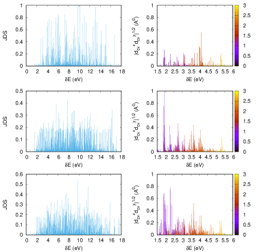
Figure 3: The top panel represents intrinsic GQD₂₁₆, the middle panel depicts GQD₂₁₆ with disorder, and the bottom panel illustrates GQD₂₁₆ with a monovacancy. The left column is the joint density of states, and the right column is the absolute values of the product of the $x$ and $y$ components of interband transition dipole matrix elements. The color boxes indicate the energy ranges (in eV) of the conduction bands.

The tensor $\sigma_{ij}\left(\omega\right)$ can be dissected into symmetric and antisymmetric components. For 2D systems, there exists a single independent component that characterizes the antisymmetric conductivity: $\sigma_{xy}\left(\omega\right)=-\sigma_{yx}\left(\omega\right)$. This component is commonly known as the dissipationless or Hall conductivity, denoted as $\sigma_{H}\left(\omega\right)$. Under spatial symmetry transformations, the Hall component transforms as a pseudo-scalar [69], given by $\sigma_{H}\left(\omega\right)=\det\left(O\right)\sigma_{H}\left(\omega\right)$. Consequently, the Hall conductivity becomes zero in systems with mirror symmetry, where $\det\left(O\right)=-1$. Furthermore, it also vanishes in time-reversal invariant systems. To observe a non-zero Hall component in the considered GQD, it is imperative to break both time-reversal and inversion symmetries. The time-reversal symmetry can be disrupted, for example, through the application of a magnetic field. Remarkably, in the context of GQDs characterized by sharp boundaries, the time-reversal symmetry is inherently broken even in the absence of an external magnetic field [6]. This intriguing property hints at the potential for Hall-type anomalous responses in such imperfect GQDs. For the purposes of our analysis, we neglect spin effects and assume a zero-temperature Fermi-Dirac distribution for initial density matrix $\varrho_{\sigma mm}^{(0)}$. Under these conditions, the expressions for the conduction tensor can be derived from Eqs. (15) and (16) as follows:

$$\sigma_{ij}\left(\omega\right)=-2i\omega\sum_{m\in\nu}\sum_{n\in c}d_{nm}^{j}d_{mn}^{i}$$

$$\times\left[\frac{1}{\varepsilon_{n}-\varepsilon_{m}-\hbar\omega-i\hbar\gamma}+\frac{1}{\varepsilon_{n}-\varepsilon_{m}+\hbar\omega+i\hbar\gamma}\right].$$ (17)

As evident from Eq. (17), the conduction tensor is primarily defined by the joint density of states (JDS):

$$JDS=\sum_{m\in\nu}\sum_{n\in c}\delta\left(\varepsilon_{n}-\varepsilon_{m}-\hbar\omega\right)$$

and the values of the product $d_{nm}^{j}d_{mn}^{i}$ of the interband transition dipole matrix elements. In Fig. 3, we illustrate the JDS and the absolute values of the product of the $x$ and $y$ components of the interband transition dipole matrix elements. As is seen from this figure, the influence of on-site disorder and a mono-vacancy on GQD₂₁₆ is nearly identical. While the JDS is somewhat suppressed, both factors lift the degeneracy of states and break the inversion symmetry, thereby opening up new channels for interband transitions. The product $d_{cv}^{x}d_{cv}^{y}$ has several peaks near the particular interband transitions, which means that near these peaks one can expect strong Hall-type anomalous response. To assess the consequences on the linear response using $\sigma_{ij}\left(\omega\right)$, we will compute the linear absorption coefficient and the Faraday rotation angle. For both quantities, we will use formulas derived for graphene at normal incidence of a laser beam. The linear absorption coefficient is defined through the diagonal component of conductivity [70]:

$$\alpha_{\mathrm{abs}}=\frac{4\pi}{c}\frac{\mathrm{Re}\sigma_{xx}\left(\omega\right)}{\left|\frac{\sqrt{\epsilon}+1}{2}+2\pi\sigma_{xx}\left(\omega\right)/c\right|^{2}},$$ (18)

while the Faraday-rotation angle $\Theta_{F}$ is related to the optical Hall conductivity [71] through the formula:

$$\Theta_{F}=\frac{1}{2}arg\left[\frac{1+\sqrt{\epsilon}+\frac{4\pi}{c}\left(\sigma_{xx}\left(\omega\right)+i\sigma_{xy}\left(\omega\right)\right)}{1+\sqrt{\epsilon}+\frac{4\pi}{c}\left(\sigma_{xx}\left(\omega\right)-i\sigma_{xy}\left(\omega\right)\right)}\right].$$ (19)

Here, $c$ represents the velocity of light, and $\epsilon$ denotes the dielectric constant of the substrate. Strictly speaking, the absorption coefficient and Faraday rotation angle are meaningful for a nanostructure layer with dimensions much larger than the incident light wavelength. In other words, we should have many copies of the GQDs uniformly distributed on a 2D surface. We investigate these quantities to emphasize the consequences of disorder or vacancies on the optical response of GQDs. In Fig. 4, we present the linear optical response of GQD₂₁₆ in terms of the absorption coefficient and Faraday rotation angle. Notably, the absorption coefficient is minimally affected by disorder or vacancies. In comparison to graphene, where $\alpha_{\mathrm{abs}}\approx{\pi}/137$, we observe a significantly higher absorption ($\alpha_{\mathrm{abs}}\sim 0.1$). In terms of Hall-type anomalous response, we observe a substantial Faraday-rotation angle for mono-vacancy and a less pronounced effect for disorder. As expected, intrinsic GQD displays a Faraday-rotation angle of zero. It is worth noting that the maximal angle induced by a mono-vacancy, $\Theta_{F}\sim 3^{{{}^{\circ}}}$, is comparable to the Faraday-rotation angle of graphene in the strong magnetic field with strengths $\sim 3\cdot 10^{4}$ Gs [72].

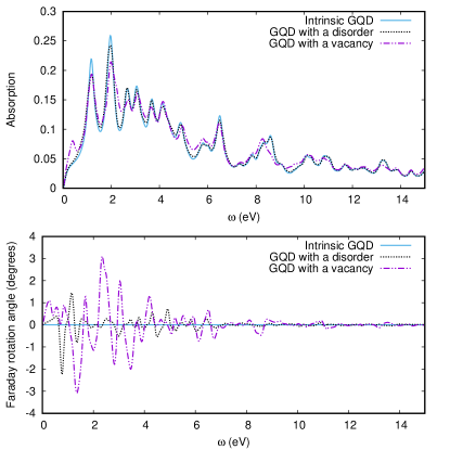
Figure 4: Linear optical response of GQD via absorption coefficient (a) and Faraday rotation angle (b). The relaxation rate is set to $\hbar\gamma=0.1\ \mathrm{eV}$. The dielectric constant of the substrate is taken to be ${\epsilon}_{d}=6$.

IV Nonlinear optical response

After considering the linear response, we begin by examining the nonlinear optical response of GQD₂₁₆ in the strong infrared laser field described by the electric field strength $\mathbf{E}\left(t\right)=f\left(t\right)E_{0}\hat{\mathbf{e}}\cos\omega t$, with the frequency $\omega$, polarization $\hat{\mathbf{e}}$ unit vector, and amplitude $E_{0}$. The wave envelope is described by the Gaussian function $f\left(t\right)=\exp\left[-2\ln 2\left(t-t_{m}\right)^{2}/\mathcal{T}^{2}\right]$, where $\mathcal{T}$ characterizes the pulse duration full width at half maximum, $t_{m}$ defines the position of the pulse maximum. Note that for the Gaussian envelope the number of oscillations $N_{s}$ of the field is approximated as $\mathcal{T}/T\simeq 0.307N_{s}$, where $T=2\pi/\omega$ is the wave period ($4.135\mathrm{fs}$ for 1$\mathrm{eV}$).

To compute the harmonic signal, we use the Fourier transform

$$\mathbf{a}\left(\Omega\right)=\int_{-\infty}^{\infty}\mathbf{a}\left(t\right)e^{i\Omega t}W\left(t\right)dt,$$ (20)

where

$$\mathbf{a}\left(t\right)=e\sum_{i\sigma}\mathbf{r}_{i}\frac{d^{2}}{dt^{2}}\rho_{ii}^{\left(\sigma\right)}\left(t\right)$$ (21)

is the dipole acceleration and $W\left(t\right)$ is a window function that suppresses small fluctuations and reduces the overall background noise of the harmonic signal [73]. We choose the pulse envelope $f\left(t\right)$ as the window function. For all further calculations we assume a polarization unit vector $\hat{\mathbf{e}}=\left\{1,0\right\}$, and the pulse duration $\mathcal{T}$ is set to $\mathcal{T}/T\simeq 3$, corresponding to approximately $10$ oscillations ($N_{s}\simeq 10$). To ensure a smooth turn-on of the interaction, we position the pulse center at $t_{m}=10T$. For convenience, we normalize the dipole acceleration by the factor $a_{0}=e\overline{\omega}^{2}\overline{d},$ where $\overline{\omega}=1\ \mathrm{eV}/\hbar$ and $\overline{d}=1\ \mathrm{\mathring{A}}$. The power radiated at a given frequency is proportional to $S\left(\Omega\right)=\left|\mathbf{a}\left(\Omega\right)\right|^{2}/a_{0}^{2}$. We perform the time integration of Eq. (6) using the eighth-order Runge-Kutta algorithm. For the Coulomb interaction matrix elements we take values from Table 1 and the dielectric constant of the substrate is taken to be ${\epsilon}_{d}=6$.

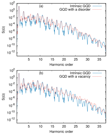
Figure 5: The total HHG spectra in logarithmic scale (in arbitrary units) for GQD₂₁₆ with a disorder (a) and for GQD₂₁₆ with monovacancy (b) along with the HHG spectra of intrinsic GQD. The wave amplitude is taken to be $E_{0}=0.3\ \mathrm{V/\mathring{A}}$. The relaxation rate is set to $\hbar\gamma=0.1\ \mathrm{eV}$. The excitation is performed assuming a laser with a wavelength of $2.48\ \mathrm{\mu m}$, an excitation frequency of $\omega=0.5\ \mathrm{eV}/\hbar$.

To begin with, we examine the effect of the mono-vacancy and disorder on the HHG spectra. The HHG spectra are compared for three different scenarios in Fig. 5: when we have the intrinsic GQD₂₁₆, when the GQD₂₁₆ has a mono-vacancy, and when it is subject to on-site disorder. The inclusion of a mono-vacancy or disorder leads to two noteworthy characteristics in the HHG spectra: (a) the most prominent feature is the emergence of even harmonics comparable to odd harmonics and (b) substantial increase in the HHG signal in the vicinity of the cutoff regime. The first phenomenon is attributed to the special inversion symmetry breaking in the presence of disorder and vacancy. The second phenomenon is connected with the fact that the disorder and vacancy lift the degeneracy of states opening up new channels for interband transitions.

To reveal the inherent effects of broken time-reversal symmetry on the nonlinear response, we conducted an investigation into polarization-resolved HHG spectra. In Fig. 6, we present the polarization-resolved HHG spectra for GQD₂₁₆ with disorder and for GQD₂₁₆ featuring a mono-vacancy. This figure highlights a significant finding, especially in the case of a mono-vacancy, where even-order harmonics manifest as Hall-type anomalous harmonics polarized perpendicular to the applied laser electric field direction.

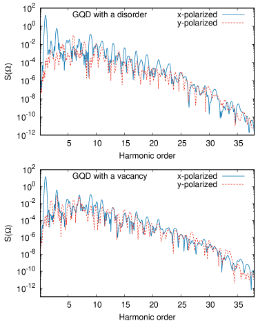
Figure 6: The polarization resolved HHG spectra in logarithmic scale for GQD₂₁₆ with a disorder (a) and for GQD₂₁₆ with a monovacancy (b). The laser parameters correspond to Fig. 5.

Of specific interest is the plateau region within the harmonics spectra. In Fig. 7, we present the plateau portion of the anomalous HHG spectrum of GQD₂₁₆ with a mono-vacancy for various wave field amplitudes. In this representation, none of the harmonics conform to the perturbation scaling $S^{1/2}\left(n\omega\right)\sim E_{0}^{n}$. This observation underscores the strictly multiphoton and nonlinear nature of the HHG process.

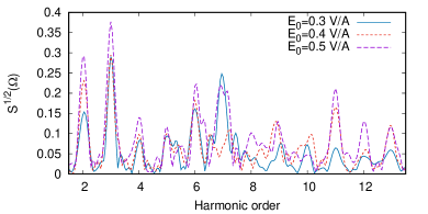
Figure 7: The plateau part of the anomalous HHG spectrum of GQD₂₁₆ with a monovacancy is presented in the linear scale for various wave field amplitudes. The excitation frequency is taken to be $\omega=0.5\ \mathrm{eV}/\hbar$.

Now, let’s consider the effect of the pump wave frequency on the Hall-type anomalous HHG process. This analysis is presented in Fig. 8 where we demonstrate the polarization-resolved HHG spectra for higher-frequency laser fields. Notably, we observe that the rate of anomalous harmonics is suppressed for higher-frequency pump waves. This phenomenon can be attributed to the fact that with higher-frequency pump waves, excitation and recombination channels predominantly involve highly excited states that still retain inversion symmetry.

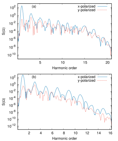
Figure 8: The polarization resolved HHG spectra in logarithmic scale for GQD₂₁₆ with a monovacancy for $\omega=1.0\ \mathrm{eV}/\hbar$ (a) and $\omega=1.5\ \mathrm{eV}/\hbar$ (b). The wave amplitude is taken to be $E_{0}=0.3\ \mathrm{V/\mathring{A}}$. The relaxation rate is set to $\hbar\gamma=0.1\ \mathrm{eV}$.

V Conclusion

We have studied the character and specifics of linear and nonlinear optical response of hexagonal GQDs in the presence of on-site disorder or vacancies. Our primary focus was on medium-sized GQDs composed of $216$ carbon atoms which in their defectless state possess inversion symmetry. To model a disorder, we employed the Anderson model, while for mono-vacancies we utilized a simplified model by setting the hopping parameters to the empty site to zero and assigning a large value to the on-site energy at the empty site. In our TB model, we considered up to the $10$th nearest-neighbor hopping elements. Electron-electron interactions were treated within the HF approximation, incorporating the long-range Coulomb interactions. Through the solution of the evolutionary equations for the single-particle density matrix, we revealed anomalous optical responses in defective GQDs across both linear and nonlinear interaction regimes. In linear response, in the absence of an external magnetic field, we observed a significant Hall conductivity, resulting in a substantial Faraday-rotation angle. This phenomenon is attributed to the intrinsic time-reversal symmetry-breaking in graphene quantum dots, coupled with the simultaneous breaking of spatial inversion symmetry in the presence of disorder or mono-vacancies. The combined disruption of time-reversal and inversion symmetries leads to the emergence of intense Hall-type anomalous HHG. Notably, these anomalous high harmonics are more pronounced in low-frequency laser fields. In such scenarios, excitation and recombination channels predominantly involve states near the Fermi level which are more susceptible to inversion symmetry breaking. Our findings underscore that even minor levels of disorder or mono-vacancy leave unique imprints in the Hall-type anomalous high harmonics, thus offering a potential avenue for optically characterizing defects in 2D nanostructures.