Accelerating the analysis of optical quantum systems using the Koopman operator

Abstract

The prediction of photon echoes is an important technique for gaining an understanding of optical quantum systems. However, this requires a large number of simulations with varying parameters and/or input pulses, which renders numerical studies expensive. This article investigates how we can use data-driven surrogate models based on the Koopman operator to accelerate this process. In order to be successful, we require a model that is accurate over a large number of time steps. To this end, we employ a bilinear Koopman model using extended dynamic mode decomposition and simulate the optical Bloch equations for an ensemble of inhomogeneously broadened two-level systems. Such systems are well suited to describe the excitation of excitonic resonances in semiconductor nanostructures, for example, ensembles of semiconductor quantum dots. We perform a detailed study on the required number of system simulations such that the resulting data-driven Koopman model is sufficiently accurate for a wide range of parameter settings. We analyze the L2 error and the relative error of the photon echo peak and investigate how the control positions relate to the stabilization. After proper training, the dynamics of the quantum ensemble can be predicted accurately and numerically very efficiently by our methods.

I INTRODUCTION

Linearization of nonlinear dynamical systems is a goal in many research areas, ranging from fluid dynamics over climate models to robotics. The Koopman operator, originally introduced by Koopman in 1931 [1], is a linear operator on the space of observables of the system. The Koopman operator not only allows for a linear representation of the nonlinear dynamics but also entails global geometric properties via its eigendecomposition. Various computational methods have been established to date, dynamic mode decomposition (DMD) and its generalization extended dynamic mode decomposition (EDMD) being two of the most popular methods. While the Koopman operator has been well-researched in general and also for particular system classes such as measure-preserving or control systems [2, 3, 4], its application in quantum physics is fairly new. Some recent investigations include [5] and [6]. Quantum-mechanical descriptions of complex systems are usually computationally challenging and numerically expensive. We examine how a Koopman operator-based model can serve as a surrogate model to conduct parameter studies on quantum systems more efficiently.
The quantum system we consider in this work is an inhomogeneously broadened ensemble of two-level systems (TLS) which describe, e.g., excitonic resonances in semiconductor quantum dots (QDs). Such systems are known to emit electromagnetic radiation in the form of photon echoes in four-wave-mixing schemes which involve impulsive excitation with two time-delayed optical pulses, see [7, 8]. Photon echoes have been proposed as a key ingredient for realizing quantum memory protocols [9] and recently it was shown that the emission time of photon echoes can be controlled optically [10, 11]. When an excitonic resonance of an inhomogeneously broadened ensemble of quantum dots, called quantum ensemble (QE), is excited by a short optical laser pulse at $t=0$, the macroscopic polarization, i.e., the sum over all individual microscopic optical polarizations, of the QE dephases. Dephasing is the rapid decay with time on a duration which is inversely proportional to the width of the distribution of transition frequencies. This dephasing can be reversed by exciting the ensemble with a second temporally delayed laser pulse at $t=\tau$. The phase conjugation induced by the second pulse leads to rephasing of the microscopic polarizations which results in the buildup of a macroscopic polarization at $t=2\tau$. This transient macroscopic polarization is the source for the emission of a pulse of electromagnetic radiation which is known as the photon echo. The contribution of this paper is to demonstrate the advantage of Koopman theory and a data-driven approximation algorithm like DMD over regular procedures in efficiency for predicting optical quantum experiments accurately over a long timescale.

II Preliminaries

II-A Quantum physical model

We consider exciton or trion transitions in ensembles of semiconductor QDs which are well described by TLS. In an ensemble of inhomogeneously broadened TLS and after the excitation with a short optical pulse, the polarizations of the individual TLS evolve with different phase velocities, due to the distribution of transition frequencies. As a result, the macroscopic polarization decays rapidly with time due to dephasing. A second pulse can induce rephasing, such that all individual polarizations are in phase again at a time which is determined by the delay of the two excitation pulses. At this time, the buildup of a macroscopic polarization leads to the emission of a so-called photon echo.
The optical properties and dynamics of near-resonantly excited TLS are obtained by solving the optical Bloch equations (OBE) in the rotating-wave approximation (RWA) [7]. The OBE describe the dynamics of electronic excitations that are driven by optical fields. They can be formulated in terms of the occupation probability $n_{l}$ of the energetically higher level and the microscopic polarization or coherence $p_{l}$ between the two levels for the $l$-th TLS, respectively. In the absence of losses they read:

$$\begin{bmatrix}\dot{p}_{l}(t)\\ \dot{n}_{l}(t)\end{bmatrix}=\begin{bmatrix}-i\delta_{l}p_{l}(t)+i\Omega_{R}(t)(1-2n_{l}(t))\\ 2\Omega_{R}(t)\imaginary(p_{l}(t))\end{bmatrix}.$$ (1)

Here, $\Omega_{R}(t)=dE(t)/\hbar$ denotes the Rabi frequency that is determined by the electric field $E(t)$, the dipole matrix element $d$ of the optical transition and the optical detuning $\delta_{l}=\omega_{l}-\omega_{L}$, which is given by the difference between the laser frequency $\omega_{L}$ and the transition frequency $\omega_{l}$ of the $l$-th TLS. We are interested in the macroscopic polarization $P(t)$ of the QE, which can be calculated as the weighted sum of all microscopic polarizations:

$$P(t):=\sum^{N}_{l=1}\sigma(\delta_{l})p_{l}(t),$$ (2)

with $N$ denoting the size of the QE, i.e., the number of considered TLS. Note that $P(t)$ is a dimensionless quantity and the physical polarization can be obtained by multiplying with $d$. In this paper, time will be denoted in picoseconds and frequencies in inverse picoseconds. The weight distribution $\sigma$ specifies the full width at half maximum (FWHM) of the distribution function modeling the inhomogeneous broadening of the transition frequencies. For our purposes, we model the energy differences between the two levels as being linearly spaced between $-R\operatorname{meV}$ and $R\operatorname{meV}$ and we refer to $R$ as the range. The discretized weight distribution for the transition detuning is as usual considered to be a Gaussian function of the form $\sigma:\mathcal{D}\rightarrow\mathbb{R}$ with

$$\sigma(\delta_{l})=\exp{-\frac{1}{2}\left(\frac{2\sqrt{2\ln{2}}\,\hbar\delta_{l}}{\operatorname{FWHM}\operatorname{meV}}\right)^{2}}.$$

Due to the discrete frequencies, unphysical repetitions in the polarization occur after the photon echo. The time of these repetitions, which are also referred to as “revival”, depends on $\sigma$ and the emission time and frequency of the laser pulses. The revival time can be calculated apriori and for the experiment as in [10] (which will also be our test case in section IV-A) it is given by:

$$T_{Rev}=\frac{2\pi(N-1)\hbar}{30\operatorname{meV}}.$$

Note that, $T_{Rev}\approx 110$ ps for $N=800$ and $T_{Rev}\rightarrow 0$ for $N\rightarrow 0$.

II-B The Koopman operator

We consider a continuous-time control system

$$\dot{x}(t)=f(x(t),u(t))$$ (3)

where $x(t)\in\mathcal{X}\subseteq\mathbb{R}^{d}$ is the system state and $u(t)\in\mathcal{U}\subseteq\mathbb{R}^{p}$ the control. The dynamics are described by the right-hand side $f:\mathcal{X}\times\mathcal{U}\rightarrow\mathbb{R}^{d}$. When $u(t)=u$ takes a constant value, we can equivalently describe the dynamics by

$$x(t+\Delta t)=\Phi^{\Delta t}_{u}(x(t)),$$ (4)

where $\Phi^{\Delta t}_{u}:\mathcal{X}\rightarrow\mathcal{X}$ is the flow map with input $u$. Whereas in general no linearity assumptions can be made about $\Phi^{\Delta t}_{u},$ the finite-time Koopman operator gives a linear description of (4) by mapping observables instead of the system states $x$. Let $\mathcal{S}$ be some space of $L^{2}$-functions on $\mathcal{X}$ that is closed under composition with the flow map. The family $\left(\mathcal{K}^{\Delta t}_{u}\right)_{\Delta t\geq 0}$ of Koopman operators on $\mathcal{S}$ for is defined by

$$\mathcal{K}^{\Delta t}_{u}\psi:=\psi\circ\Phi^{\Delta t}_{u}$$ (5)

for all $\psi\in\mathcal{S}$. The Koopman family is a semigroup if $\left(\Phi^{\Delta t}_{u}\right)_{\Delta t\geq 0}$ is a semigroup, see [12]. When considering the continuous system (3), we can instead work with the generator of the semigroup [13]:

$$\mathcal{K}_{u}\psi:=\lim_{\Delta\rightarrow 0}\frac{\mathcal{K}^{\Delta t}_{u}\psi-\psi}{\Delta t}\quad\forall\psi\in\mathcal{D}(\mathcal{K}_{u}),$$ (6)

where $\mathcal{D}(\mathcal{K}_{u}):=\{\psi\in\mathcal{S}:\;\text{the limit in }\eqref{eq:def_koopman_generator}\text{ exists}\}$. Inserting (5) into $\eqref{eq:def_koopman_generator}$, one obtains

$$\mathcal{K}_{u}\psi(x(t)) =\lim_{\Delta t\rightarrow 0}\frac{\psi(x(t+\Delta t)-\psi(x(t))}{\Delta t}$$

$$=\frac{d}{dt}\psi(x(t))=\dot{x}(t)\cdot\nabla_{x}\psi(x(t)),$$

which yields

$$\mathcal{K}_{u}\psi=f\cdot\nabla_{x}\psi.$$

Hence, the Koopman generator $\mathcal{K}_{u}$ differentiates observables with respect to the dynamics, whereas the finite-time operators $\mathcal{K}^{\Delta t}_{u}$ evolve observables one time step forward. To approximate the Koopman operator, one commonly chooses a set of functions $\Psi=\{\psi_{1},\dots,\psi_{z}\}$ like eigenfunctions or generic basis functions such as polynomials or radial basis functions to generate the function space $\mathcal{S}=\operatorname{span}(\psi_{1},\dots,\psi_{z})$.

II-B1 Control-affine systems

Suppose the system in (3) is control-affine

$$\dot{x}(t)=f(x(t),u)=g(x(t))+h(x(t))\cdot u,$$ (7)

with $g:\mathcal{X}\rightarrow\mathcal{X}$ and ${h(x(t))\cdot u:=\left(\sum_{j=1}^{p}h_{j}(x(t))u^{(j)}\right)}$, where $h_{j}:\mathcal{X}\rightarrow\mathcal{X}$ and $u^{(j)}\in\mathbb{R}$ is the j-th coordinate of $u$. In this case, Koopman theory is especially convenient, because the control affinity of the system state translates to the Koopman generator, resulting in a bilinear model. This will be the main idea for the algorithms in section III and is based on the observations in [14]. To see this, one recognizes that the Koopman generator for a constant control $u\in\mathcal{U}$ on the system (7) give ${\mathcal{K}_{u}\psi=g\cdot\nabla_{x}\psi+h\cdot u\cdot\nabla_{x}\psi}$. When introducing a linear combination of constant controls $u=\sum_{i=1}^{c}\alpha_{i}u_{i}$ where $\alpha_{i}\in\mathbb{R}$, this becomes

$$\mathcal{K}_{u}\psi =g\cdot\nabla_{x}\psi+\sum_{j=1}^{p}h_{j}\cdot\sum_{i=1}^{c}\alpha_{i}u_{i}\cdot\nabla_{x}\psi$$ (8)

$$=\sum_{i=1}^{c}\alpha_{i}\left(h\cdot u_{i}\right)\cdot\nabla_{x}\psi.$$

Note the special case of the unactuated state $\mathcal{K}_{0}\psi=g\cdot\nabla_{x}\psi$. If we define $\mathcal{B}_{u}:=\mathcal{K}_{u}-\mathcal{K}_{0}$, then $\mathcal{B}_{u}\psi=h\cdot u\cdot\nabla_{x}\psi$ and we may write (8) as

$$\mathcal{K}_{u}=\mathcal{K}_{0}+\sum_{i=1}^{c}\alpha_{i}\mathcal{B}_{u_{i}}.$$

If we choose basis vectors $e_{1},\dots,e_{p}\in\mathbb{R}^{p}$ as control points ($c=p$), then $u=\sum_{i=1}^{p}u^{(i)}e_{i}$ and we obtain the bilinear system

$$\mathcal{K}_{u}z(t)=\left(\mathcal{K}_{0}+\sum_{i=1}^{c}u^{(i)}\mathcal{B}_{e_{i}}\right)z(t).$$ (9)

Eq. (9) can also be generalized to time-dependent control $u(t)$. By choosing a representation with linear factors $u(t)=\sum_{i=1}^{c}u_{i}(t)e_{i}$, we obtain the following analogous to (9):

$$\mathcal{K}_{u(t)}z(t)=\left(\mathcal{K}_{0}+\sum_{i=1}^{c}u_{i}(t)\mathcal{B}_{e_{i}}\right)z(t).$$ (10)

The algorithms in section III approximate the finite-time operators $\mathcal{K}^{\Delta t}$ instead of $\mathcal{K}_{u}$. Instead of the exact model in Eq. (10), the finite-time analog is only accurate up to first order in $\Delta t$:

$$\mathcal{K}^{\Delta t}_{u(t)}=\mathcal{K}^{\Delta t}_{0}+\sum_{i=1}^{c}u_{i}(t)\mathcal{B}^{\Delta t}_{e_{i}}+\mathcal{O}(\Delta t^{2}).$$

This implies that a reduced-order model based on Koopman operators induces an error even if the underlying dynamics are bilinear as in the case of the OBE. However, if the underlying dynamics are not bilinear, the finite-time model tends to be more efficient numerically, as we do not need to integrate in time.

III Algorithms

We propose two algorithms based on [14], which construct a bilinear Koopman model for control-affine systems using EDMD. We will refer to this method as bilinear EDMDc. DMD, has become a popular technique to approximate the Koopman generator because it is purely data-driven and computationally efficient even for high-dimensional data. To approximate the Koopman operator (e.g. compute a finite-rank operator), linear observations of the state space are collected instead of system states. The relaxation of linear observables leads to EDMD [15] and also the constraint for evenly spaced time points can be relaxed. Other methods based on (E)DMD for control systems can for example be found in [16] and [17]. The procedure in [14] coincides with other EDMD methods in that the Koopman generators are approximated on the space of observables spanned by an a priori fixed set of nonlinear basis functions $\Phi$, called “dictionary”. The distinguishing idea in [14] is the approximation of a set of Koopman generators, each with respect to a fixed actuation, and the construction of a bilinear model by interpolating the generators with respect to the target actuation. Note that the OBE (1) establish a bilinear system themselves, thus direct linearization would in principle be possible. That is, the Koopman generators can be computed exactly. Nonetheless, we give algorithms to compute the finite-time Koopman operators as we aim to provide methods that are applicable to a broad class of possibly nonlinear systems in the optical quantum area.

(a)

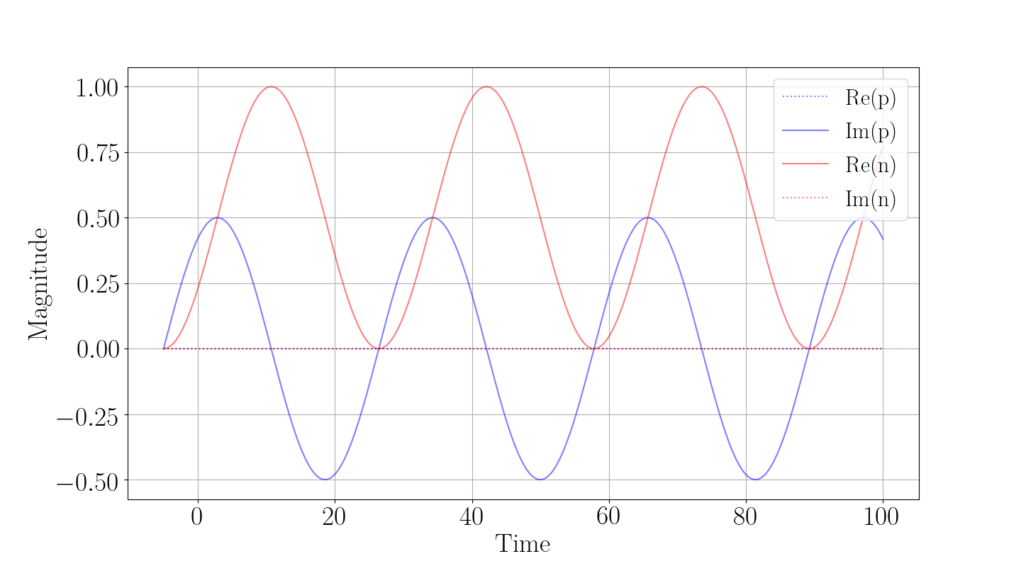
(b)

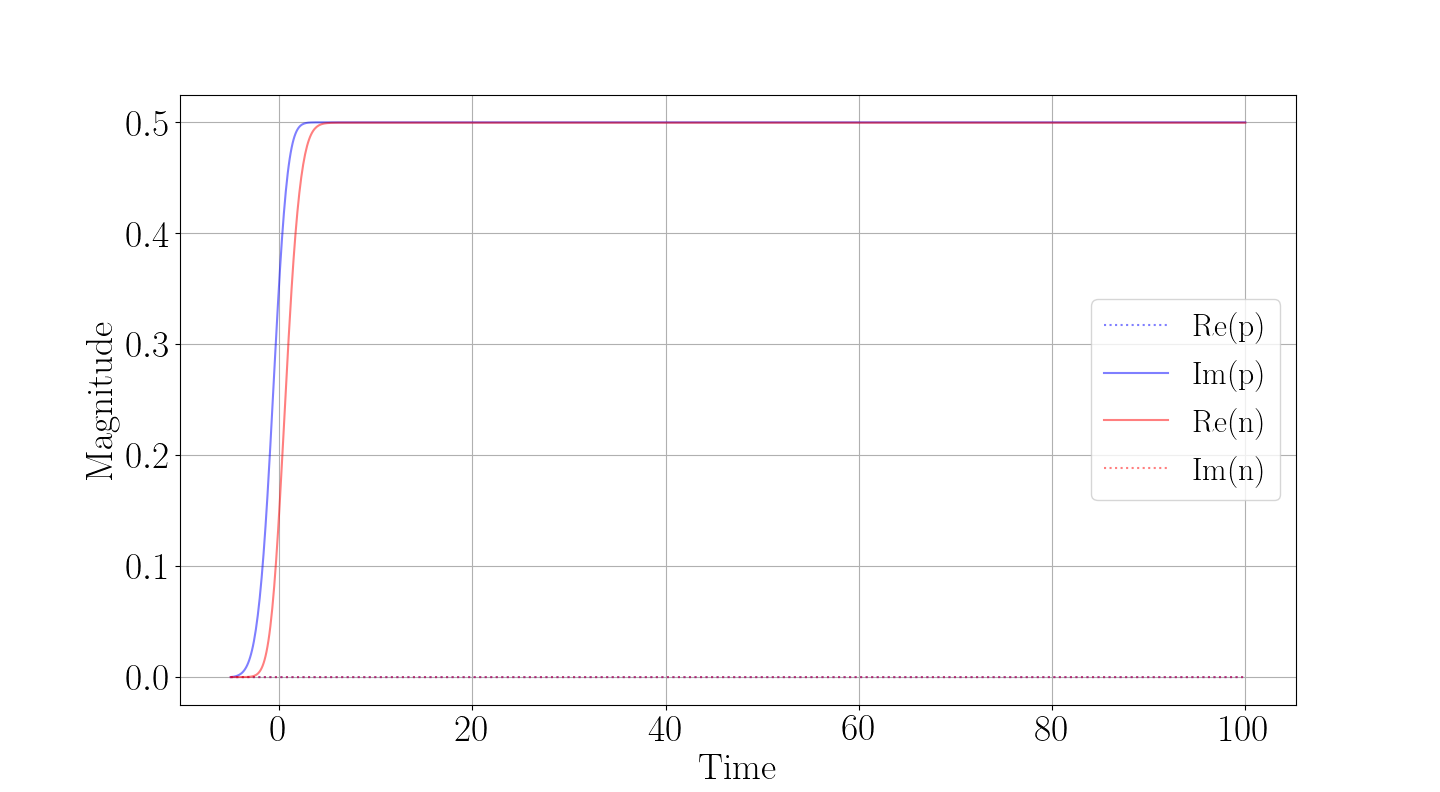
(c)

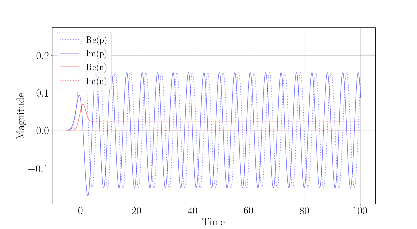
Figure 1: Solutions of the OBE with respect to different laser pulses and detunings. (a) Constant pulse with amplitude $0.2$, i.e., $\Omega_{R}(t)=0.2\Theta(t)/$, where $\Theta$ is the Heaviside function, and detuning $\delta=0\operatorname{meV}$. (b), (c) Gaussian pulse with area $\frac{\pi}{2}$ and duration $2.5$, detuning $\delta=0\operatorname{meV}$ and $\delta=0.75\operatorname{meV}$, respectively.

III-A Bilinear EDMDc

Training the bilinear EDMD algorithm works as follows:

1. Fix $c+1$ control points $\mathbf{U}=\{\mathbf{0},\mathbf{u}_{1},\dots,\mathbf{u}_{c}\}$, dictionary $\Psi=\{\psi_{1},\dots,\psi_{z}\}$ and time points $\{t_{1},\dots,t_{n}\}$. Set the time step $\Delta t$ for integration.

2. Collect the initial system states $\mathbf{x}_{i}:=\mathbf{x}(t_{i})$ in a matrix $\mathbf{X}$ and lift $\mathbf{X}$ to

   $$\Psi(\mathbf{X})=\begin{bmatrix}|&&|\\ \Psi(\mathbf{x}_{1})&\dots&\Psi(\mathbf{x}_{n})\\ |&&|\end{bmatrix}\in\mathbb{R}^{z\times n}.$$

3. Calculate $\mathbf{G}:=\left(\Psi(\mathbf{X})\Psi(\mathbf{X})^{\top}\right)^{\dagger}.$

4. For every control point $\mathbf{u}\in\mathbf{U}$:

   1. Generate the propagated system states ${\mathbf{x}^{\prime}_{\mathbf{u},i}:=\Phi^{\Delta t}_{\mathbf{u}}(\mathbf{x}_{i})}$ by solving the differential equations and build corresponding matrices $\mathbf{X}^{\prime}_{u}$.

   2. Calculate $\mathbf{A_{\mathbf{u}}}:=\Psi(\mathbf{X})\Psi(\mathbf{X}^{\prime}_{\mathbf{u}})^{\top}.$

   3. Approximate the Koopman operators by

      $$\mathbf{K}^{\Delta t}_{\mathbf{u}}=\left(\mathbf{G}\mathbf{A_{\mathbf{u}}}\right)^{\top}.$$

During Prediction, we then simply do:

1. Compute $\mathbf{K}^{\Delta t}_{\mathbf{u}(t_{i})}=\mathbf{K}^{\Delta t}_{\mathbf{0}}+\sum_{j=1}^{c}\alpha_{j}(t_{i})\mathbf{B}^{\Delta t}_{\mathbf{u}_{j}}$.

2. Predict via $\Phi^{\Delta t}_{\mathbf{u}(t_{i})}\Psi(\mathbf{x}(t_{i}))\approx\mathbf{K}^{\Delta t}_{\mathbf{u}(t_{i})}\Psi(\mathbf{x}(t_{i}))$.

III-B BE and BERG

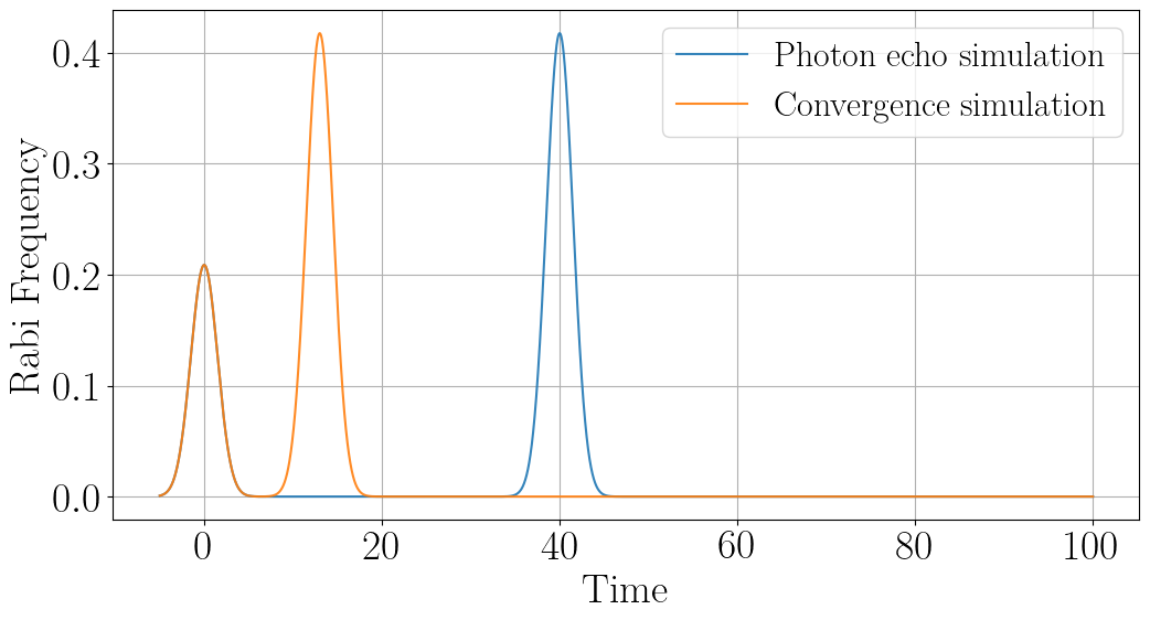
Figure 2: The optical pulses used in the experiments.

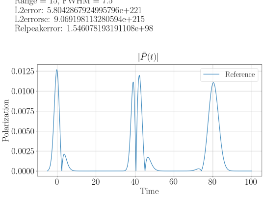
Figure 3: The polarization in the first simulation. The photon echo occurs at $t=80$.

To fit bilinear EDMDc to the simulation of the OBE, we note that (1) is affine-linear in the system state and choose $\Psi$ as the set of monomials up to order $1$, i.e. we only add a bias term in contrast to standard DMD. Besides the system state, the OBE entail the one-dimensional Rabi frequency $\Omega_{R}(t)$ as a time-dependent control parameter and the one-dimensional detuning $\delta$ as a constant parameter. The difficulty in producing an accurate model for the OBE lies in capturing the dynamics for the entire quantum ensemble, consisting of TLS with varying detunings, excited by an arbitrary laser pulse with varying $\Omega_{R}(t)$. Fig. 1 exemplifies how $\Omega_{R}(t)$ and $\delta$ influence the solution of the OBE. We model the detuning as one coordinate of the time-dependent control and create a bilinear model with respect to the two-dimensional control $u(t)=\left[\Omega_{R}(t),\delta\right]$. If we define $\mathbf{\Omega}$ and $\mathbf{D}$ to be the discretized grid of training points for $\Omega_{R}$ and $\delta$ respectively, we have $\mathbf{U}=\mathbf{\Omega}\times\mathbf{D}$ and both accuracy, as well as computational efficiency of the resulting model, are ultimately determined by the refinement of the training grids and the time step size. For both algorithms, we split $p$ and $n$ into real and imaginary parts and construct $n=100$ random initial system states in $\left[-1,1\right]^{4}$, before solving the OBE with a Runge-Kutta method of order $4$ and time step $\Delta t$.

III-B1 Bilinear EDMD (BE)

In the first approach we choose control points $\mathbf{U}=\{\left[0,0\right],\left[1,0\right],\left[0,1\right]\}$, $c=2$. Since $\mathbf{u}(t_{i})=\Omega_{R}(t_{i})\left[1,0\right]+\delta\left[0,1\right]$, the prediction at time point $t_{i}$ is given by

$$\mathbf{K}^{\Delta t}_{\mathbf{u}(t_{i})}\mathbf{x}(t_{i})=\left(\mathbf{K}^{\Delta t}_{\left[0,0\right]}+\Omega_{R}(t_{i})\mathbf{B}^{\Delta t}_{\left[1,0\right]}+\delta\mathbf{B}^{\Delta t}_{\left[0,1\right]}\right)\mathbf{x}_{i}.$$

Section IV-A will show that this model is not stable in certain parameter settings, due to the inaccuracies introduced by EDMD in the discrete-time setting. This motivates the introduction of additional control points.

III-B2 BE on refined grid (BERG)

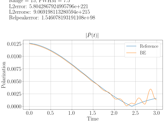
Figure 4: BE in simulation 1 for $R=15$ and $t=1$ to $t=3$.

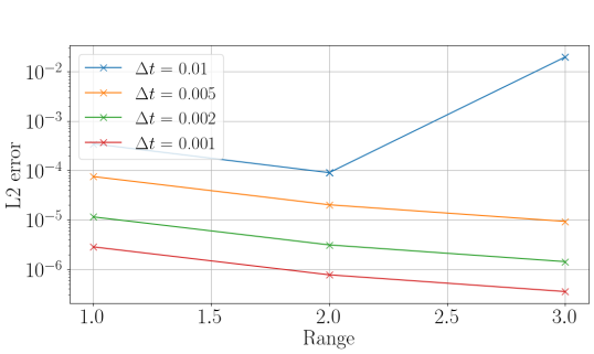
Figure 5: L2 error of BE against the detuning range and for different step sizes.

The training control points in BERG have the form $\mathbf{U}=\mathbf{\Omega}\times\mathbf{D}$, where $\mathbf{\Omega}=\left[0,1\right]$ as before, but $\mathbf{D}$ consists of $m$ values between $-R$ and $R$. That is, $\mathbf{D}$ is a coarser instantiation of the test detunings $\mathcal{D}$. In contrast to the single, global BE model, we now construct a family of bilinear models parameterized by $\mathcal{D}$, where each model interpolates between the two detuning parameters closest to the corresponding test detuning. Consider a fixed test control $u=\left[\omega_{i},\delta_{i}\right]$ and let $\delta_{1},\delta_{2}\in\mathbf{D}$ be the two training detunings that are closest to $\delta_{i}$ with respect to Euclidean distance. Using $a\in\left[0,1\right]$, we obtain $\delta_{i}=(1-a)\delta_{1}+a\delta_{2}$. Then $\left[\omega_{i},\delta_{i}\right]=\omega_{i}\left[1,0\right]+(1-a)\left[0,\delta_{1}\right]+a\left[0,\delta_{2}\right]$ and

$$\mathbf{K}^{\Delta t}_{\left[\omega_{i},\delta_{i}\right]} =\mathbf{K}^{\Delta t}_{\left[0,0\right]}+\omega_{i}\left(\mathbf{K}^{\Delta t}_{\left[1,0\right]}-\mathbf{K}^{\Delta t}_{\left[0,0\right]}\right)$$

$$+(1-a)\left(\mathbf{K}^{\Delta t}_{\left[0,\delta_{1}\right]}-\mathbf{K}^{\Delta t}_{\left[0,0\right]}\right)$$

$$+a\left(\mathbf{K}^{\Delta t}_{\left[0,\delta_{2}\right]}-\mathbf{K}^{\Delta t}_{\left[0,0\right]}\right)$$

$$=\mathbf{K}^{\Delta t}_{\left[0,0\right]}+\omega_{i}\mathbf{B}^{\Delta t}_{\left[1,0\right]}+\mathbf{B}^{\Delta t}_{\left[0,\delta\right]}$$

for the Koopman operator, where we abbreviated $\mathbf{B}^{\Delta t}_{\left[0,\delta\right]}:=(1-a)\mathbf{K}^{\Delta t}_{\left[0,\delta_{1}\right]}+a\mathbf{K}^{\Delta t}_{\left[0,\delta_{2}\right]}-\mathbf{K}^{\Delta t}_{\left[0,0\right]}.$

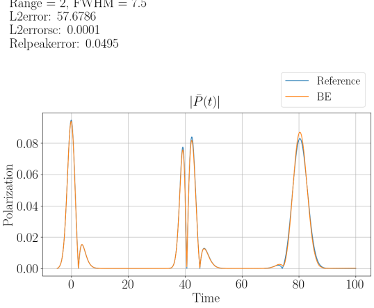
Figure 6: BE in the first simulation with $R=2$.

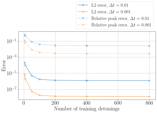
Figure 7: L2 error and relative peak error of BERG in simulation 1 for different step sizes.

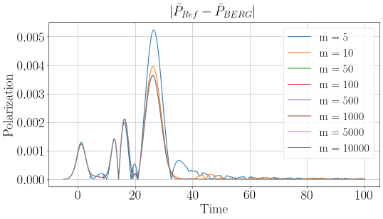
Figure 8: Difference between normalized polarization of reference and BERG in the second simulation.

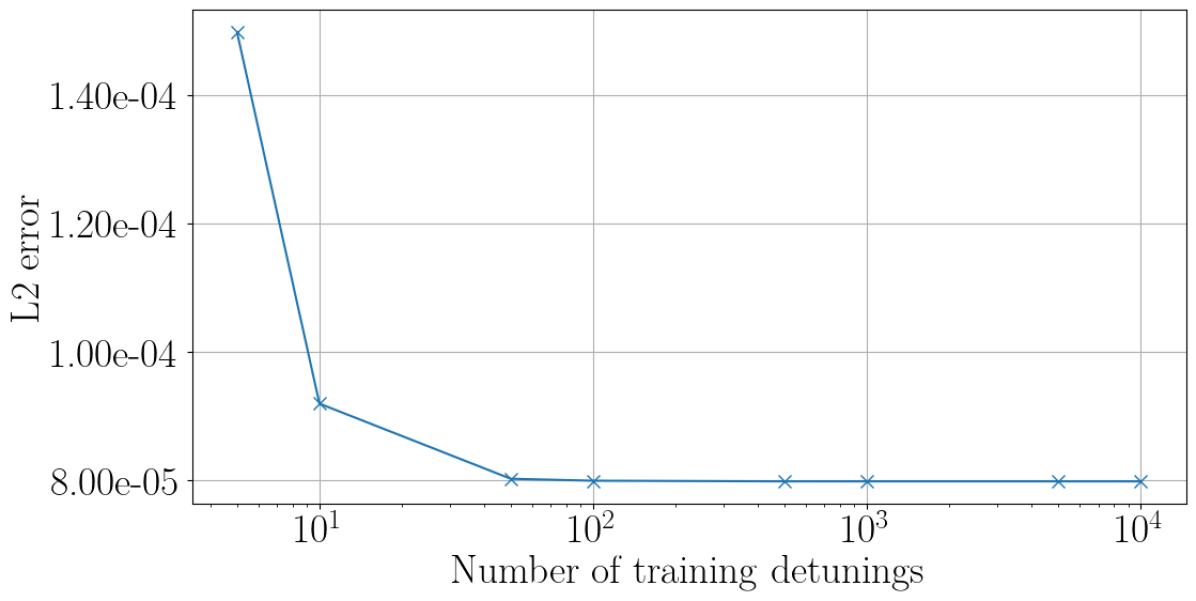
(a)

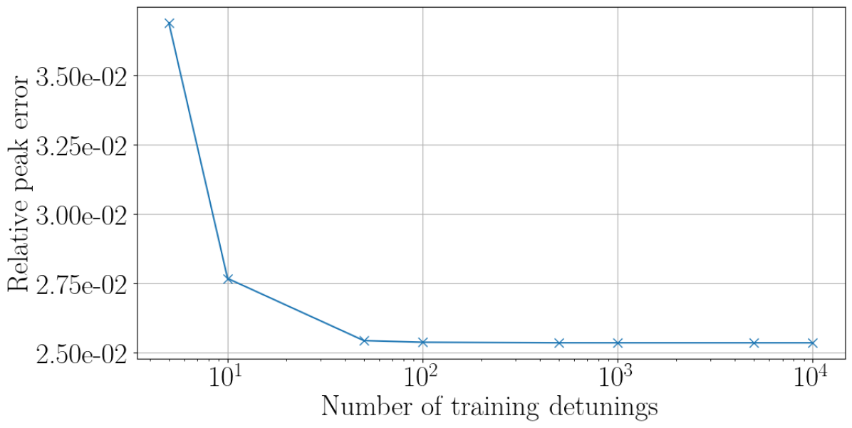
(b)

Figure 9: (a) L2 error and (b) relative peak error for BERG in simulation 2. In both cases, $m+1$ detunings were trained, where $m\in\{5,10,50,100,500,1000,5000,10000\}$.

IV Results

IV-A The photon echo

We perform two simulations with the Koopman models. Our first goal is to test how accurately BE simulates the polarization in a photon echo scheme as demonstrated in [10]. In this reference, the QE consists of $N=800$ TLS with evenly spaced detunings in the range $R=15$ and a weight distribution $\sigma$ with $\operatorname{FWHM}=7.5$ meV. The exciting pulse is composed of an initial $\frac{\pi}{2}$-pulse of duration $2.5$, centered at $t=0$ and a second pulse with pulse area $\pi$, centered at $t=40$ with the same duration. The pulses of both simulations can be found in Fig. 2. The reference data is computed by solving the OBE with SciPy’s solve_ivp() function using RK45 [18], parameters $\Delta t=0.01$, $\text{rtol}=1e-8$ and $\text{atol}=1e-11$ for the interpolation. An illustration of the reference solution for the first simulation can be found in Fig. 3. The polarization is calculated according to (2) and evaluation occurs from $t=-5$ to $t=100$. For the evaluation, we choose two error measures that are invariant under the size of the ensemble $N$, as this variable will vary in simulation 2 IV-B. We aim to quantify both the overall error as well as the deviation of the model in the photon echo peak. Let $\bar{P}(t)=\frac{P(t)}{N}$ be the normalized polarization, then the respective L2 error is given by

$$L_{2}(\bar{P}_{Ref},\bar{P}_{BE})=\int^{t=100}_{t=-5}\left(\frac{P_{Ref}(t)}{N}-\frac{P_{BE}(t)}{N}\right)^{2}dt,$$

where $P_{R}$ and $P_{BE}$ denote the macroscopic polarization of the reference and BE, respectively. We write $S_{Ref}$ and $S_{BE}$ for the photon echo peak of the reference and BE and consider the relative peak error

$$L_{peak}(P_{Ref},P_{BE})=\left|\frac{S_{Ref}-S_{Be}}{S_{Ref}}\right|.$$

When evaluating BE with these parameter settings and a step size of $\Delta t=0.01$, the model quickly deviates from the reference calculation, see Fig. 4. Although the reduction of the step size to $\Delta t=0.001$ slightly decreases the L2 error, BE does not suffice to model the original experiment. When deviating from the original experiment and varying the detuning range, we observe that the L2 error is dependent on the considered range of detunings, see Fig. 5. For $\Delta t=0.01$ the lowest L2 error is attained at $R=2$ with $L_{2}\approx 9.01\cdot 10^{-5}$. With these parameters BE matches the reference trajectory and also approaches the photon echo peak, which is supported by the relative peak error $L_{Peak}\approx 0.05$, see Fig. 6. However, for greater ranges, i.e. $R\geq 4$, the L2 error explodes and BE therefore is not relevant for the prediction of the OBE in general. We derive that, although the underlying dynamics are comparatively simple, the large number of time steps in combination with the control input pose substantial challenges, implying that the modeling process needs to be performed carefully. The larger number of detunings $m$ that we collect training data for in BERG serves to decrease the interpolation error. The trade-off between $m$ and the error measures is illustrated in Fig. 7. The results for the two error measures are similar and we can derive two conclusions. First, it is apparent that the step size has a great impact on the error, and second, $m=100$ and $m=200$ appear to provide an excellent trade-off between accuracy and data requirements. E.g. for step size $\Delta t=0.01$, we obtain $L_{2}\approx 1.75\cdot 10^{-6},L_{Peak}\approx 0.039$ with $m=100$ and $L_{2}\approx 1.34\cdot 10^{-6},L_{Peak}\approx 0.029$ using $m=200$. Thus, by choosing an appropriate number of training detunings, BERG is able to simulate the photon echo experiment with an error that can be adjusted with the step size.

IV-B Convergence with QE size

The second simulation serves to investigate the convergence of the photon echo with the number of QDs in the QE. Since in reality, $N$ is very large, it is extremely costly to perform detailed simulations for all QDs, we learn the Koopman model from $m\ll N$ trajectories. We fix $N=10^{4}$ and $\Delta t=0.01$. For evaluation, we compare the relative peak error of the Koopman model, trained on $m$ detunings and tested on $N$ detunings with the relative peak error of a reference calculation of $N$ detunings. Since we include data from the classical integration of a small-sized QE and $T_{Rev}\rightarrow 0$ for $N\rightarrow 0$, there is a need to tune the parameters such that $T_{Rev}>100$ even for small $N$. The resulting parameters are given by $R=1$ and weight distribution with $\operatorname{FWHM}=1$ meV. The pulse is shown in Fig. 2. To illustrate the results, Fig. 8 shows the difference in the reference polarization and the polarization calculated by BERG for different $m$. The error visualization can be found in Fig. 9. We examine that the trajectories of L2 error and relative peak error of BERG are similar to the corresponding error data of simulation 1. While we evaluated $m$ in correspondence to $N=10^{4}$, and thus $m$ takes different values than in simulation 1, we again observe an obvious dip in the error measures. In this simulation, the dip occurs with fewer training detunings, at $m=10$ ($L_{2}=9.19\cdot 10^{-5},L_{Peak}=0.027$) and $m=50$ ($L_{2}=8.103\cdot 10^{-5},L_{Peak}=0.025$), implying that we have reduced the number of expensive simulations by a factor of $100$.

V Conclusions

We have investigated the possibility of using Koopman operator-based surrogate models to accelerate the analysis of optical quantum systems. Even though the original system has bilinear dynamics, the small inaccuracies of the discrete-time bilinear Koopman model pose significant challenges for long-term predictions such that special care has to be taken during modeling. By introducing a refined training grid for the detuning, stabilization of the model can be achieved, leading to accurate predictions of TLS in an RWA. Several aspects of training the bilinear model may still be investigated. For example, the effect of other sampling techniques for the detuning control instances has yet to be determined, in distinction to the effect of the linearly spaced detunings that we applied. A refined grid for the optical pulse may reduce error measures further. The increasing interest in quantum systems will require further research for efficient simulation and control. We illustrated the potential of a Koopman operator-based model in quantum applications by giving accuracy results on a simple quantum system, but more complex quantum systems still need to be investigated. Examples include the nonlinear optical dynamics of electronic many-body systems or the ultrafast dynamics of matter driven with extremely strong fields, providing access to attosecond time scales.

References

- [1] B. O. Koopman, “Hamiltonian systems and transformation in hilbert space,” Proceedings of the National Academy of Sciences of the United States of America, vol. 17, no. 5, pp. 315–318, may 1931.
- [2] S. L. Brunton, M. Budišić, E. Kaiser, and J. N. Kutz, “Modern koopman theory for dynamical systems,” SIAM Review, vol. 64, no. 2, pp. 229–340, may 2022.
- [3] S. E. Otto and C. W. Rowley, “Koopman operators for estimation and control of dynamical systems,” Annual Review of Control, Robotics, and Autonomous Systems, vol. 4, no. 1, pp. 59–87, May 2021.
- [4] A. Mauroy, I. Mezic, and Y. Susuki, The Koopman Operator in Systems and Control Concepts, Methodologies, and Applications: Concepts, Methodologies, and Applications. Springer, 2020.
- [5] S. Klus, F. Nüske, and S. Peitz, “Koopman analysis of quantum systems,” Journal of Physics A: Mathematical and Theoretical, vol. 55, no. 31, p. 314002, jul 2022.
- [6] I. Mezić, “A transfer operator approach to relativistic quantum wavefunction,” Journal of Physics A: Mathematical and Theoretical, vol. 56, no. 9, p. 094001, feb 2023.
- [7] L. Allen and J. Eberly, Optical Resonance and Two-level Atoms. Wiley, New York, 1975.
- [8] T. Meier, P. Thomas, and S. Koch, Coherent Semiconductor Optics: From Basic Concepts to Nanostructure Applications. Springer, New York, 2006).
- [9] V. Damon, M. Bonarota, A. Louchet-Chauvet, T. Chanelière, and J.-L. L. Gouët, “Revival of silenced echo and quantum memory for light,” New Journal of Physics, vol. 13, no. 9, p. 093031, sep 2011.
- [10] A. N. Kosarev, H. Rose, S. V. Poltavtsev, M. Reichelt, C. Schneider, M. Kamp, S. Höfling, M. Bayer, T. Meier, and I. A. Akimov, “Accurate photon echo timing by optical freezing of exciton dephasing and rephasing in quantum dots,” Communications Physics, vol. 3, dec 2020.
- [11] S. Grisard, A. V. Trifonov, H. Rose, R. Reichhardt, M. Reichelt, C. Schneider, M. Kamp, S. Höfling, M. Bayer, T. Meier, and I. A. Akimov, “Temporal sorting of optical multiwave-mixing processes in semiconductor quantum dots,” ACS Photonics, vol. 10, no. 9, pp. 3161–3170, 2023.
- [12] B. Farkas and H. Kreidler, “Towards a koopman theory for dynamical systems on completely regular spaces,” Phil. Trans. R. Soc. A, vol. 378, no. 2185, 11 2020.
- [13] S. Klus, F. Nüske, S. Peitz, J.-H. Niemann, C. Clementi, and C. Schütte, “Data-driven approximation of the Koopman generator: Model reduction, system identification, and control,” Physica D: Nonlinear Phenomena, vol. 406, p. 132416, 2020.
- [14] S. Peitz, S. E. Otto, and C. W. Rowley, “Data-driven model predictive control using interpolated koopman generators,” SIAM Journal on Applied Dynamical Systems, vol. 19, no. 3, pp. 2162–2193, sep 2020.
- [15] M. O. Williams, I. G. Kevrekidis, and C. W. Rowley, “A data–driven approximation of the koopman operator: Extending dynamic mode decomposition,” Journal of Nonlinear Science, vol. 25, pp. 1307–1346, jun 2015.
- [16] J. L. Proctor, S. L. Brunton, and J. N. Kutz, “Dynamic mode decomposition with control,” SIAM Journal on Applied Dynamical Systems, vol. 15, no. 1, pp. 142–161, jan 2016.
- [17] M. O. Williams, M. S. Hemati, S. T. M. Dawson, I. G. Kevrekidis, I. G. Kevrekidis, and C. W. Rowley, “Extending data-driven koopman analysis to actuated systems,” IFAC-PapersOnLine, vol. 49, no. 18, pp. 704–709, dec 2016.
- [18] P. Virtanen, R. Gommers, T. E. Oliphant, M. Haberland, T. Reddy, D. Cournapeau, E. Burovski, P. Peterson, W. Weckesser, J. Bright, S. J. van der Walt, M. Brett, J. Wilson, K. J. Millman, N. Mayorov, A. R. J. Nelson, E. Jones, R. Kern, E. Larson, C. J. Carey, İ. Polat, Y. Feng, E. W. Moore, J. VanderPlas, D. Laxalde, J. Perktold, R. Cimrman, I. Henriksen, E. A. Quintero, C. R. Harris, A. M. Archibald, A. H. Ribeiro, F. Pedregosa, P. van Mulbregt, and SciPy 1.0 Contributors, “SciPy 1.0: Fundamental Algorithms for Scientific Computing in Python,” Nature Methods, vol. 17, pp. 261–272, Feb 2020.