ATCA Study of Small Magellanic Cloud Supernova Remnant 1E 0102.2–7219

Abstract

We present new and archival Australia Telescope Compact Array and Atacama Large Millimeter/submillimeter Array data of the Small Magellanic Cloud supernova remnant 1E 0102.2–7219 at 2100, 5500, 9000, and 108000 MHz; as well as Hi data provided by the Australian Square Kilometre Array Pathfinder. The remnant shows a ring-like morphology with a mean radius of 6.2 pc. The 5500 MHz image reveals a bridge-like structure, seen for the first time in a radio image. This structure is also visible in both optical and X-ray images. In the 9000 MHz image we detect a central feature that has a flux density of 4.3 mJy but rule out a pulsar wind nebula origin, due to the lack of significant polarisation towards the central feature with an upper limit of 4 per cent. The mean fractional polarisation for 1E 0102.2–7219 is $7\pm 1$ and $12\pm 2$ per cent for 5500 and 9000 MHz, respectively. The spectral index for the entire remnant is $-0.61\pm 0.01$. We estimate the line-of-sight magnetic field strength in the direction of 1E 0102.2–7219 of $\sim$44 $\mu$G with an equipartition field of $65\pm 5\,\mu$G. This latter model, uses the minimum energy of the sum of the magnetic field and cosmic ray electrons only. We detect an Hi cloud towards this remnant at the velocity range of $\sim$160–180 km s^-1 and a cavity-like structure at the velocity of 163.7–167.6 km s^-1. We do not detect CO emission towards 1E 0102.2–7219.

1 Introduction

The Small Magellanic Cloud (SMC) is a gas-rich irregular dwarf galaxy orbiting the Milky Way (MW) with a current star formation rate of 0.021–0.05 M_⊙ yr^-1 (For et al., 2018). As the second nearest star-forming galaxy after the Large Magellanic Cloud (LMC), its relatively small distance of $\sim$60 kpc (Hilditch et al., 2005; Graczyk et al., 2020) and low Galactic foreground absorption ($N_{\rm HI}\sim 6\times 10^{20}$ cm^-2) enables supernova remnants (SNRs) to be studied in great detail (Crawford et al., 2008). These remains of stellar explosions are characterised by strong non-thermal radio-continuum emission (e.g. Hurley-Walker et al., 2021; Bozzetto et al., 2023) whose analysis provides a greater understanding of stellar evolution and the distribution of heavy elements (e.g. Filipović & Tothill, 2021).

1E 0102.2–7219 (hereafter referred to as E0102) is a young (1738$\pm$175 yr) core-collapse SMC SNR (van den Bergh, 1988; Banovetz et al., 2021), discovered via X-ray observations taken by the Einstein Observatory (Seward & Mitchell, 1981). At X-ray wavelengths, E0102 presents a bright, filled ring-like structure with an outer edge that traces the forward-moving blast wave (Stanimirović et al., 2005). The bright X-ray ring shows strong emission lines of O, Ne and Mg, which are in the region between the reverse shock and the contact discontinuity with the ISM, revealing significant substructure (Gaetz et al., 2000; Sasaki et al., 2006). E0102 is thought to originate from a core-collapse supernova scenario, given its ‘oxygen-rich’ nature observed in the optical band (Dopita et al., 1981). Flanagan et al. (2004) calculated the oxygen mass in the ejecta to be 6 $M_{\odot}$ using Chandra X-ray data, estimating a total progenitor mass of 32 $M_{\odot}$. Progenitor mass estimates from $\sim$40 $M_{\odot}$ using data from the Chandra archive (Alan et al., 2019) to greater than 50 $M_{\odot}$ using Hubble Space Telescope (HST) data (Finkelstein et al., 2006) have been suggested.

Amy & Ball (1993) published the first radio study of E0102, presenting two images using the Molonglo Observatory Synthesis Telescope (MOST) at 843 MHz and the Australia Telescope Compact Array (ATCA) at 4790 MHz. The ATCA image showed a $\sim$40 arcsec diameter ring-like source (resolution = $2.75\times 2.96$ arcsec², root mean square (RMS) noise = $\sim$75 $\mu$Jy beam^-1) and the authors estimated a radio spectral index of $-0.7$.

Here, we present new high-resolution and high-sensitivity radio-continuum observations of E0102 obtained from ATCA and the Atacama Large Millimeter/submillimeter Array (ALMA). The general flow of our study of E0102 is as follows. Section 2 is a description of radio observations, data acquisition and initial analysis from the ATCA, Australian Square Kilometre Array Pathfinder (ASKAP), Chandra, HST, Multi-Unit Spectroscopic Explorer (MUSE), and ALMA telescopes. Next, Section 3 explores further analysis and results including radio morphology, polarisation, spectral index, rotation measure, magnetic field, and Hi / CO morphology. Section 4 is a discussion of the implications from our analysis, including the environment of E0102 and a comparison with other young SNRs. Final thoughts and conclusions are given in Section 5.

2 Observations

2.1 ATCA observations

Our new (2019-2021) and archival ATCA observations are listed in Table 1, including: observing date, project code, array configuation, number of channels, bandwidth, frequency, phase and flux calibrator used, and integrated time. All were carried out in ‘snap-shot’ mode, with 1-hour integrations over a 12-hour period minimum, using the Compact Array Broadband Backend (CABB) (2048 MHz bandwidth) centred at wavelengths of 3/6 cm and 13 cm ($\nu$ = 2100 MHz). Total integration times were $\sim$575 minutes and $\sim$1410 minutes, respectively. Complementary array configurations (Table 1) achieved good $uv$ coverage, including long (6A, 6C, and 6D), mid (1.5C), and short (EW367) baselines, essential to imaging the full extent of E0102. The result of using such configurations is that our shortest baseline measured just 45.9 m (array EW367) and the longest reaching 5938.8 m (array 6A). In contrast, Amy & Ball (1993) only utilised five of the six antennas, with a minimum baseline of 76.5 m and the longest at 2525.5 m – which significantly affected the quality of the image given the limited $uv$ coverage.

We used miriad (Sault et al., 1995), karma (Gooch, 1995), and DS9 (Joye & Mandel, 2003) software packages for reduction and analysis. All observations were calibrated using the phase and flux calibrators as listed in Table 1 with one iteration of phase-only self-calibration using the selfcal task. To best image the diffuse emission emanating from the SNR, we experimented with a range of various values for weighting and tapering. We found Briggs weighting robust parameter of –2 (uniform weighting) the most optimal choice. We add a Gaussian taper to further enhance the diffuse emission (1 arcsec at 5500 MHz and 1.5 arcsec at 9000 MHz) which resulted in a resolution of $2\times 2$ arcsec² for these images. The mfclean and restor algorithms were used to deconvolve the images, with primary beam correction applied using the linmos task. To increase the S/N ratio for weak polarisation emission, we follow the same process with stokes Q and U parameters but with a beam size of $5\times 5$ arcsec² (see Section 3.3 for more details).

Table 1: Summary of SNR E0102 ATCA observations used in this study.

Observing	Project	Array	No.	Bandwidth	Frequency $\nu$	Phase	Flux	Integrated time
Date	Code	Config.	Channels	(GHz)	(MHz)	Calibrator	Calibrator	(minutes)
04 Jan 2012	C2521	6A	2049	2.048	2100	PKS B0230–790	PKS B1934–638	1410.1
04 Jan 2015	CX310	6A	2049	2.048	5500,9000	PKS B0230–790	PKS B1934–638	37.8
22 Dec 2017	CX403	6C	2049	2.048	5500,9000	PKS B0230–790	PKS B0252–712	193.2
20 Jun 2019	C3293	6A	2049	2.048	5500,9000	PKS B0230–790	PKS B1934–638	119.4
04 Dec 2019	C3275	1.5C	2049	2.048	5500,9000	J0047–7530	PKS B1934–638	46.2
21 Feb 2020	C3296	EW367	2049	2.048	5500,9000	PKS B0230–790	PKS B1934–638	75.6
26 Feb 2021	C3403	6D	2040	2.048	5500,9000	PKS B0530–727	PKS B1934–638	102.6

2.2 Hi observations

The Hi data used in this study are from Pingel et al. (2022). These Hi data (1420.4 MHz) were obtained using the ASKAP with an angular resolution of $30\times 30$ arcsec², corresponding to a spatial resolution of $\sim$9 pc at the distance of the SMC. The typical noise fluctuations of the Hi data cube are $\sim$1.1 K at a velocity resolution of 0.98 km s^-1.

2.3 Chandra observations

We analysed archival X-ray data obtained using Chandra with the Advanced CCD Imaging Spectrometer. We combined 142 individual observations from August 1999 (ObsID: 138) to February 2021 (ObsID: 24579) using Chandra Interactive Analysis of Observations (CIAO; Fruscione et al., 2006) software version 4.12 with CALDB 4.9.1 (Graessle et al., 2007). The data were reproduced using the chandra_repro procedure. Using the ‘merge_obs’ procedure in the energy band of 0.5–7.0 keV, we produced an exposure-corrected, energy-filtered image. The total effective exposure time is $\sim$1570 ks.

2.4 HST observations

The [O iii] filter HST image of E0102 was downloaded from the Mikulski Archive for Space Telescopes. Information about these HST observations and their data reduction are detailed in Blair et al. (2000).

2.5 MUSE observations

The [Fe xiv] image of E0102 was created as a slice through the IFU datacube from observations on 7^th October 2016 using MUSE under ESO program 297.D-5058 (PI: F. P. A. Vogt). All details regarding these MUSE observations and their data reduction are found in Vogt et al. (2017).

2.6 ALMA observations

We utilised archival datasets from both continuum and CO line emissions obtained using ALMA. The 3 mm continuum observations centred at 108058 MHz were carried out using the 12-m array as a cycle 6 project (PI: F. Vogt, #2018.1.01031.S). The correlator was set with four spectral windows 1875 MHz wide, centred at 101125, 103000, 113125, and 115000 MHz. Observations consisted of two executions with 48 and 45 antennas in a compact array configuration with baselines ranging between 15.1 and 500.2 m which correspond to maximum recoverable scales of $\sim$16 arcsec (following Eq. 7.7 in the ALMA Cycle 8 Technical Handbook Cortes et al., 2020). We used the products delivered by the pipeline processed with the Common Astronomy Software Application (CASA; McMullin et al., 2007) package version 5.4.0-70 and Pipeline version 42254 (Pipeline-CASA54-P1-B). Imaging incorporated a Briggs robust value of 1.0. The ALMA radio continuum image covers a total bandwidth of 7290 MHz and achieved an RMS of 31 $\mu$m. The beam size is $2.46\times 1.93$ arcsec² with a position angle of 0$\aas@@fstack{\circ}$73 corresponding to a spatial resolution of $\sim$0.6 pc at the distance of the SMC. Additional observations with a more extended configuration were available in the archive but since no continuum was detected at higher resolution, they were not included. Spectral line emission ¹²CO (J = 1–0), covered by one of the spectral windows in this dataset, is not detected.

Since spatial filtering may be significant (see section 3.3 in the ALMA Cycle 8 Technical Handbook of Cortes et al., 2020), the line emission ¹²CO (J = 2–1) was obtained with the Atacama Compact Array (ACA, a.k.a. Morita Array) comprising the 7-m ALMA antennas and 12 m total power array, carried out as a wide field survey in Cycle 5/6 (PI: C. Agliozzo, #2017.A.00054.S). The baselines ranging from 9 to 48 m result in maximum recoverable scales of 27 arcsec. Additionally, this survey allows us to explore a wider region, comparable to the Hi dataset (see Section 3.6). The whole dataset, beyond the region used in this study, has been published by Tokuda et al. (2021). Details on data reduction, imaging and combination between interferometric data and single-dish observations can be found in Tokuda et al. (2021). The final beam size is $6.87\times 6.56$ arcsec² with a position angle of 39$\aas@@fstack{\circ}$09, corresponding to a spatial resolution of $\sim$2 pc at the distance of the SMC. The typical noise fluctuation is $\sim$66 mK at the velocity resolution of 0.5 km s^-1.

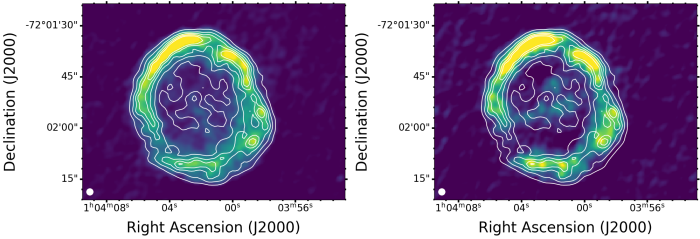
Figure 1: Images of SNR E0102 with 2100 MHz contours overlaid from 500 to 2500 $\mu$Jy beam^-1 at increments of 500 $\mu$Jy beam^-1. Left: ATCA intensity image at 5500 MHz. Right: ATCA image at 9000 MHz. The white circles on the lower left corner in both images represent a synthesised beam of $2\times 2$ arcsec².

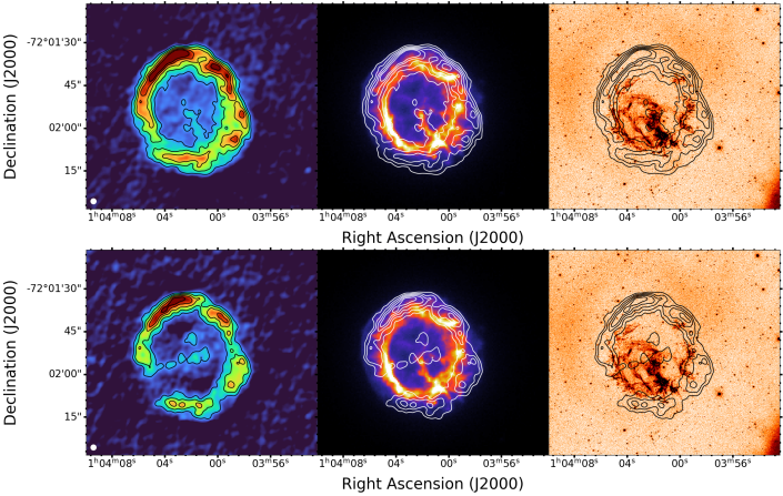
Figure 2: Images of SNR E0102 with 5500 MHz contours overlaid (top) and 9000 MHz contours overlaid (bottom). The contour levels are from 200 to 1000 $\mu$Jy beam^-1 at increments of 200 $\mu$Jy beam^-1. Left: ATCA intensity image at 5500 MHz (top) and 9000 MHz (bottom). The white circles on the lower left corner represent a synthesised beam of $2\times 2$ arcsec². Middle: Broadband Chandra X-ray images. Right: HST [O iii] filter images (Blair et al., 2000).

3 Analysis

3.1 Morphology

Our new ATCA images of E0102 clearly show a ring-like structure with bright emissions in the north-west and north-east regions (Fig. 1). A comparison between the high-resolution radio continuum (ATCA) images of SNR E0102 at 5500 and 9000 MHz and other wavelength images is presented in Fig. 2. The RMS noise for 5500 MHz and 9000 MHz images are $\sim$30 and 48 $\mu$Jy beam^-1, respectively. In this Section, we describe how we calculate the centre and the radius of E0102, compare our new images with X-ray and optical images, and list new features seen for the first time in radio images.

3.1.1 Centre and radius calculation

We used the Minkowski tensor analysis tool BANANA (Collischon et al., 2021) to determine the centre of expansion. This tool searches for filaments and calculates normal lines and line density maps. For a perfect shell, all lines should meet at the centre position inside the SNR, where the expansion must have started (see Collischon et al., 2021, for more details). Since real sources deviate from this ideal picture, we circumvented this problem by smoothing the line density map using a circle with a diameter of 40 pixels. We then took the centre position of the pixel where the line density was the highest. Using the same method, we performed the tensor analysis separately for the 5500 MHz, 9000 MHz, and Chandra broad-band images. From this, we calculated the mean centre position and the $1\sigma$ uncertainty of the mean. The resulting calculated centre is RA (J2000) = 01^h04^m02.23^s, Dec (J2000) = $-$72^∘01$\arcmin$53$\aas@@fstack{\prime\prime}$06 with an uncertainty of $\sim$0.91 arcsec. This is $\sim$1.5 arcsec ($\sim$0.4 pc at the distance of 60 kpc) north-west from the previous estimation of RA (J2000) = 01^h04^m02.48^s, Dec (J2000) = $-$72^∘01$\arcmin$53$\aas@@fstack{\prime\prime}$92, having a $1\sigma$ uncertainty of 1.77 arcsec (Banovetz et al., 2021). The latter was derived from HST observations of the proper motion of optical ejecta. Therefore, our calculated position agrees well with previous estimates, within uncertainties.

To estimate the radio continuum radius of E0102, we used the miriad task cgslice to plot 16 equispaced radial profiles in 22.5^∘ segments around the remnant at 5500 MHz. Each profile is 30 arcsec in length (Fig. 3). We divide the remnant into four equal regions: south-west (profiles 1–5), south-east (profiles 5–9), north-east (profiles 9–13), and north-west (profiles 13–1) (Fig. 3, A). We identified the cutoff as the point where each profile intersects the outer contour line ($3\sigma$ ATCA image contour or 200 $\mu$Jy beam^-1 at 5500 MHz). These cutoffs are represented as dashed vertical lines (see Fig. 3, B, C, D, and E). The thick black vertical lines represent the average of the cutoffs in each region. The resulting radii vary from $23.7\pm 01.7$ arcsec ($6.9\pm 0.5$ pc) towards the south-west (Fig. 3, B) to $20.9\pm 02.1$ arcsec towards the south-east ($6.1\pm 0.6$ pc; Fig. 3, C) and $20.0\pm 0.9$ arcsec ($5.8\pm 0.3$ pc) towards the north-east (Fig. 3, D) to $20.9\pm 0.4$ ($6.1\pm 0.1$ pc) towards the north-west (Fig. 3, E) with an average of $21.4\pm 01.3$ arcsec ($6.2\pm 0.4$ pc) for the entire SNR.

Using the same methodology we estimate the X-ray radii based on the Chandra image (Fig. 4). The radii vary from $21.1\pm 01.3$ arcsec ($6.1\pm 0.4$ pc) towards the south-west (Fig. 4, B) to $18.6\pm 0.4$ arcsec ($5.4\pm 0.1$ pc) towards the south-east (Fig. 4, C) and $20.7\pm 01.1$ arcsec ($6.0\pm 0.3$ pc) towards the north-east (Fig. 4, D) to $21.7\pm 0.4$ arcsec ($6.3\pm 0.1$ pc) towards the north-west (Fig. 4, E) with an average of $20.5\pm 0.8$ arcsec ($5.1\pm 0.2$ pc).

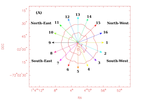
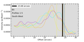
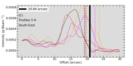
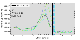
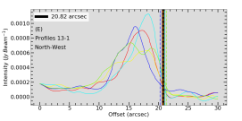
Figure 3: Estimate of the radio continuum radius of E0102 at 5500 MHz. A: Radial profiles around the remnant from the centre (see Section 3.1) overlaid on the $\bm{3\sigma}$ ATCA image contour (200 $\mu$Jy beam^-1) at 5500 MHz. The central position of the remnant is RA (J2000) = 01^h04^m02.35^s, Dec (J2000) = $-$72^∘01$\arcmin$52$\aas@@fstack{\prime\prime}$11. B, C, D, and E: Radial profiles. The dashed vertical lines represent profile cutoffs and the thick black vertical lines represent the average of the cutoffs (in arcsec) for different parts of the shell; south-west, south-east, and north-east, and north-west, respectively.

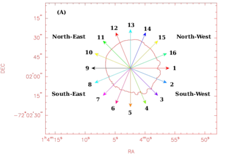
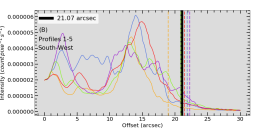
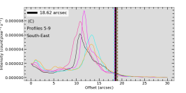
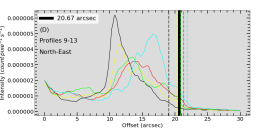
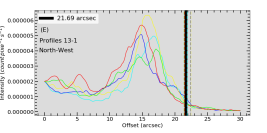
Figure 4: Estimate of X-ray radius of E0102. A: Radial profiles overlaid on $3\sigma$ Chandra broadband X-ray image contour ($6\times 10^{-7}$ counts pixel^-1s^-1). The central position of the remnant is RA (J2000) = 01^h04^m02.40^s, Dec (J2000) = $-$72^∘01$\arcmin$53$\aas@@fstack{\prime\prime}$42. B, C, D, and E: Radial profiles. The dashed vertical lines represent profile cutoffs and the thick black vertical lines represent the average of the cutoffs (in arcsec) for different parts of the shell; south-west, south-east, north-east, and north-west, respectively.

3.1.2 Radio vs. X-ray vs. optical

A comparison of our new ATCA data (Section 2.1) with the Chandra X-ray image (Section 2.3) and optical HST image (Section 2.4) reveals that the radio/X-ray maximum does not correlate well, while there is no apparent correlation with optical emission either. In the similar age Galactic SNR Vela Jr (G266.2–1.2), Stupar et al. (2005) and Maxted et al. (2018) observed the opposite, where radio emission is trailing behind the X-ray emission.

Fig. 5 (left) shows radio emission extends beyond X-ray emission, as it most likely traces the forward shock while X-ray emission could be a tracer of reverse shocked gas (Gaetz et al., 2000). Further, some of the radio profiles (e.g. 2, 6, 8) show secondary peaks offset towards the centre of the remnant. These second peaks, however, have a larger radius than the X-ray emission, indicating a second radio ring in parts of the remnant that can be associated with the amplified magnetic field that is expected at the contact-discontinuity (CD) between the shocked ejecta and shocked ISM (Jun & Norman, 1996; Zirakashvili et al., 2014).

Interestingly, we note that the [Fe xiv] emission is sandwiched between radio and X-ray emission (see Fig. 5, right). We suggest we see two phases of clumpy medium: the forward shock (a fast blast wave of a few 1000 km s^-1) and denser parts of circumstellar medium (CSM)/ISM (where the blast wave is driving slower cloud shocks). The [Fe xiv] emission is coming from shocks with velocities around 340 km s^-1 (Vogt et al., 2017). It takes some finite time for the shocked material in the denser clumps to be ionised behind the cloud shock giving us the iron lines we see; during that time the blast wave has already raced ahead, placing spatial separation between the two emitting regions. The two bright sources near the centre of the remnant and all point sources in the field are stars (Fig. 5, right).

3.1.3 Bridge like structure

We note a striking similarity of a ‘bridge-like structure’ feature between our 5500 MHz (ATCA) and the Chandra image, which projects from the centre of the remnant and connects to the south-west side of the E0102 ring. However, it is comparatively less prominent in HST image (see Fig. 2, upper panel). This feature is not detected at 9000 MHz and is likely the result of interactions with an interstellar cloud seen in Spitzer and Herschel data and similar to that seen in LMC SNR N49 (Otsuka et al., 2010). This structure was not seen in 4790 MHz image reported by Amy & Ball (1993).

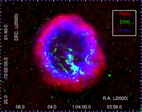
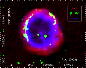
Figure 5: Red-Green-Blue (RGB) image of the E0102 SNR, with the key printed in the upper right-hand corner. Left: Our 5500 MHz ATCA data are in red, the HST image ([O iii] filter) in green (Blair et al., 2000), and the Chandra broadband image is in blue. Right: 5500 MHz ATCA data are in red, the smoothed MUSE image ([Fe xiv]) in green (Vogt et al., 2017), and the Chandra broadband image is in blue.

3.1.4 Central region

Another interesting feature that we detect exclusively in our 9000 MHz image is a horizontal bridge or bar-like feature in the central region with a measured flux density of 4.3 mJy. This feature is prominent across the interior of the SNR starting at the Eastern shell going almost all the way to the Western shell (see Fig. 2, lower panel). The fact that this structure is observed across multiple array configurations with the ATCA, and on different dates, suggests this to be a real and interesting additional feature. This structure was not seen in the previous 8640 MHz observations, likely due to lower sensitivity and poor $uv$ converge. We are unable to conclusively deduce its true nature due to the limited sensitivity of our images at 9000 MHz. Possible explanations may include a pulsar wind nebula (PWN) or jet-like features from a runaway pulsar. Further observations are required to draw any definitive conclusions.

3.2 Spectral index

The radio spectrum of an SNR can often be described as a pure power-law of frequency: $S_{\nu}$ $\propto$ $\nu^{\alpha}$, where $S_{\nu}$ is the flux density, $\nu$ is the frequency, and $\alpha$ is the spectral index.

We used the miriad (Sault et al., 1995) task imfit to extract a total integrated flux density from all available radio continuum observations of SNR E0102 listed in Table 2. This includes observations from the Murchison Widefield Array (MWA), MOST (Clarke et al., 1976; Turtle et al., 1998), ASKAP, ATCA (Filipović et al., 2002) and ALMA. We measured the MWA flux density for each sub-band (76–227 MHz) and we also re-measured the ASKAP flux density at 1320 MHz from Joseph et al. (2019). For cross-checking and consistency, we used aegean (Hancock et al., 2018) and found no significant difference in integrated flux density estimates. Namely, we measured E0102 local background noise (1$\sigma$) and carefully selected the exact area of the SNR which also excludes all obvious unrelated point sources. We then estimated the sum of all brightnesses above 5$\sigma$ of each individual pixel within that area and converted it to SNR integrated flux density following Findlay (1966, eq. 24). We also estimate that the corresponding radio flux density errors are below 10 per cent as examined in our previous work (Filipović et al., 2022; Bozzetto et al., 2023). In this estimate, various contributions to the flux density error are considered including missing short spacings. While for weaker sources this uncertainty is more proclaimed, for brighter objects such as our SNR E0102, the flux density error is much smaller ($<$10 per cent).

In Fig. 6 we present the flux density vs. frequency graph for E0102. The relative errors are used for the error bars on a logarithmic plot. The best power-law weighted least-squares fit is shown (thick black line), with the spatially integrated spectral index $\langle\alpha\rangle=-0.61\pm 0.01$ which is somewhat flattened compared to the value of $\alpha=-0.7$ reported in the previous study of Amy & Ball (1993), and consistent with the value of the similar aged LMC SNR N 132D of $-0.65\pm 0.04$ (Bozzetto et al., 2017).

Table 2: E0102 flux density measurements used in this study (see Fig. 6). The asterisk (^∗) indicates that we re-measured this flux density. Note that the flux density values for the spectral index plot shown in (Maggi et al., 2019) are based on measurements as explained in Section 3.2.

$\nu$	$S_{\nu}$	Telescope	Reference
(MHz)	(Jy)
76	1.327	MWA	This work
84	1.281	MWA	This work
88	1.386	MWA	This work
92	1.261	MWA	This work
99	1.179	MWA	This work
107	1.305	MWA	This work
115	1.152	MWA	This work
118	1.161	MWA	This work
122	1.138	MWA	This work
130	1.121	MWA	This work
143	1.087	MWA	This work
151	1.074	MWA	This work
155	0.937	MWA	This work
158	1.026	MWA	This work
166	1.004	MWA	This work
174	0.939	MWA	This work
181	0.993	MWA	This work
189	0.915	MWA	This work
197	0.903	MWA	This work
200	0.790	MWA	This work
204	0.885	MWA	This work
212	0.868	MWA	This work
220	0.888	MWA	This work
227	0.857	MWA	This work
408	0.650	MOST	Maggi et al. (2019)
843	0.396	MOST	Maggi et al. (2019)
960	0.402	ASKAP	Joseph et al. (2019)
1320	0.317∗	ASKAP	Joseph et al. (2019)
1420	0.273	ATCA	Maggi et al. (2019)
2100	0.220	ATCA	This work
2370	0.195	ATCA	Maggi et al. (2019)
4790	0.112	ATCA	Amy & Ball (1993)
4800	0.114	ATCA	Maggi et al. (2019)
5500	0.131	ATCA	This work
8640	0.082	ATCA	Maggi et al. (2019)
9000	0.083	ATCA	This work
16700	0.050	ATCA	Maggi et al. (2019)
108000	0.009	ALMA	This work

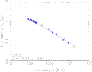
Figure 6: Radio continuum spectrum of E0102.

3.2.1 Spectral index image

We produced a spectral index map for E0102 using 2100, 5500 and 9000 MHz images (Fig. 7). To do this, the images were re-gridded to the finest image pixel size ($0.3\times 0.3$ arcsec²) using the miriad task regrid. These were smoothed to the lowest data resolution ($2.7\times 2.6$ arcsec²) using the miriad task convol. The miriad task maths then created the spectral index map (Fig. 7).

The mean value of the spectral index across the entire SNR is $-0.54\pm 0.11$. Most areas near the circumference (see Fig. 7) have a steep spectral index ($\alpha=-0.6$) at both inner and outer radii, while indices with flat gradients are found at intermediate radii ($\alpha=-0.1$). The north-east region is different in that there is no steepening at the largest radii but near zero gradients. The radio emission is brightest in the north-east with a close match between brighter emission and near zero spectral gradients. The fractional polarisation (see Section 3.3) shown in Fig. 8 is not well correlated with areas exhibiting steeper spectral indices.

We suggest that we are seeing a geometrical projection effect. The radio emission comes from the forward shock region with higher energy electrons (with larger diffusion length) spread over a wider range in radius. This yields a flattened radio spectra further from the shock. The radio emission is also sensitive to the strength and orientation of the magnetic field, so SNRs tend to have patchy radio emission (more so than the X-ray emission). This is seen in radio images of most Galactic SNRs (e.g. see the radio images posted on SNRcat) where they consist of partial shells or filaments. Adding this patchiness at different radii, we see the whole thing in projection on the sky. If the centre of a bright patch happens to be on the projected SNR’s rim, the flat spectral index region can be seen distinctly. But in most cases the bright patch, although on the surface of the 3D SNR, will not be on the rim so we see a combination of flat and steep spectral indices along the line of sight. For E0102 the brightest patch (north-east) happens to be nearly perfectly perpendicular to our line-of-sight, which would be a rare occurrence among SNRs. Finally, there are steeper spectral index regions ($-1.0<\alpha<-0.8$) towards the south-west and east SNR ring in the so-called SNR break-out regions similar to those seen in MCSNR 0455–6838 (Crawford et al., 2008).

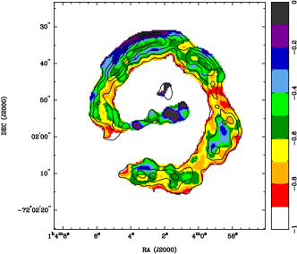
Figure 7: Spectral index map of E0102 (ATCA 2100, 5500, and 9000 MHz images with 9000 MHz contour lines overlaid). The contour levels are the same as Fig. 2. The colour bar on the right-hand side represents the gradients of the spectral index.

3.3 Polarisation

The fractional polarisation ($P$) can be calculated using the equation:

$$P=\frac{\sqrt{S^{2}_{Q}+S^{2}_{U}}}{S_{I}},$$ (1)

where $P$ is the mean fractional polarisation; $S_{Q}$, $S_{U}$, and $S_{I}$ are intensities for the $Q$, $U$, and $I$ Stoke parameters, respectively.

We used the miriad task impol to produce polarisation maps. The fractional polarisation from E0102 appears prominent at both 5500 MHz and 9000 MHz towards the north-east and north-west of the SNR, due to interactions with the local ISM. The west and south-west remnant both show slight polarisation. The polarisation vector maps at both 5500 MHz and 9000 MHz are presented in Fig. 8 as well as the polarisation intensity maps at each frequency.

We estimate a mean fractional polarisation of $7\pm 1$ per cent at 5500 MHz and $12\pm 2$ per cent at 9000 MHz, with a peak value at the centre of the bright north-eastern shell of $9\pm 1$ per cent and $26\pm 6$ per cent, respectively. The fractional polarisation of E0102 is somewhat higher than the 4 per cent (4790 MHz) (Dickel & Milne, 1995) value of similar age ($\sim$2500 yr; Law et al., 2020) oxygen-rich LMC SNR N 132D. We did not detect any significant polarisation towards the bridge-like structure and the central region, with upper limits of 2 and 4 per sent for 5500 and 9000 MHz, respectively. This lack of polarisation argues against a PWN scenario for this emission, as PWNs are typically associated with strong polarisation (e.g., Haberl et al., 2012; Brantseg et al., 2014).

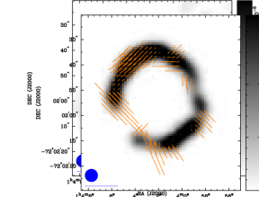
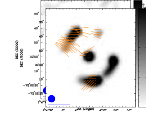
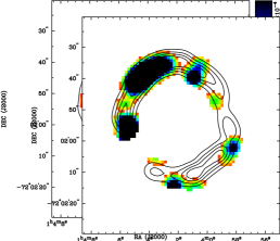
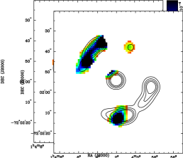
Figure 8: Fractional polarisation vectors of E0102 overlaid on intensity ATCA image at 5500 MHz (upper left) and at 9000 MHz (upper right). The blue circle in the lower left corner represent a synthesised beam of $5\times 5$ arcsec² and the blue line below the circle represents 100 per cent polarisation. The bar on the right side represents the grayscale gradients for the ATCA images in Jy beam^-1. Polarisation intensity maps of E0102 at 5500 MHz (bottom left) and at 9000 MHz (bottom right) with intensity image contour lines overlaid. The contour levels are 0.001, 0.002, 0.003, and 0.004 Jy beam^-1 for both images. The colour bar represents gradients of polarisation intensity in Jy beam^-1.

3.4 Rotation measure

One way to estimate the line-of-sight magnetic field in the direction of E0102 is by finding its rotation measure ($RM$) using $Q$ and $U$ maps at 5500 and 9000 MHz, convolved to a common resolution of 4 arcsec.

The rotation measure is defined as the slope of the observed position angle ($\phi$) as a function of wavelength ($\lambda$) squared:

$$RM=\frac{d\phi(\lambda^{2})}{d\lambda^{2}},$$ (2)

To calculate the $RM$ and intrinsic polarisation angle maps we used the program rmcalc from the DRAO export software package (Higgs et al., 1997).

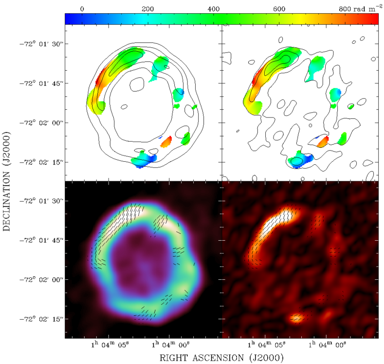
Figure 9: Top: $RM$ map calculated between the observations at 5500 MHz and 9000 MHz with overlaid contours of total power (left) and polarised intensity (right) at 5500 MHz. Bottom: Images of total power (left) and polarised intensity (right) with overlaid vectors in B-field direction, corrected for Faraday rotation.

The final $RM$ map is shown in Fig. 9. We only calculated $RM$ where the signal-to-noise ratio in the polarised intensity maps was at least $10\sigma$ at both frequencies. We notice that all $RM$ values are positive, with a maximum of almost $1000\pm 25$ rad m^-2 at the outer edge of the bright north-eastern shell and a minimum of about 0 rad m^-2 at the bottom of the SNR. One striking feature is a $RM$ gradient along the bright shell in the north-east, which could indicate the expansion into a homogenous interstellar magnetic field (Kothes & Brown, 2009). The foreground contribution of the MW is about +23 rad m^-2 according to Mao et al. (2008), based on a $RM$ study of polarised background sources that are behind the SMC. Contributions from inside the SMC are not clear as the latest study of the SMC’s internal magnetic field structure (Livingston et al., 2022) did not have any samples in the area around E0102. They found slightly more negative than positive $RM$s, and most of those sources are in positive and negative clusters.

Once the $RM$ has been determined, we next rotated the polarisation vectors back to their intrinsic (zero wavelength) values. In Fig. 9 we have added an additional 90$\degr$ to the intrinsic electric vectors, so the vectors represent the magnetic-field directions in the remnant projected to the plane of the sky. In the shell of E0102, we find segments with tangential and radial magnetic fields, representing later and earlier phases of evolution, respectively. Most striking is the tangential magnetic field related to the prominent north-eastern part of the SNR’s shell, where we also found the $RM$ gradient.

3.5 Magnetic fields in E0102

Observed rotation measure can help better understand the line-of-sight magnetic field in the direction of E0102. Useful to this discussion is first exploring an independent method known as equipartition or minimum-energy. This method uses modeling and simple parameters to estimate intrinsic magnetic field strength and energy contained in the magnetic field and cosmic ray particles using radio synchrotron emission (Arbutina et al., 2012, 2013; Urošević et al., 2018).

This approach is a purely analytical method, described as an order of magnitude estimate because of errors in determination of distance, angular diameter, spectral index, a filling factor, and flux density, tailored especially for the magnetic field strength in SNRs. Arbutina et al. (2012, 2013); Urošević et al. (2018) present two models; the difference is composition of assumed cosmic ray particles. In their original "$\kappa\neq 0$" model, where $\kappa$ is a constant in the power-law energy distributions for electrons, cosmic rays are assumed to be composed of electrons, protons and ions. Their "$\kappa=0$" model assume cosmic rays composed of electrons only. Urošević et al. (2018) showed the latter type of equipartition is superior to the former.

Using the Urošević et al. (2018) model, the mean equipartition field over the whole E0102 remnant is $65\pm 5$ $\mu$G, with an estimated minimum energy of $E_{\rm min}=1\times 10^{49}$ erg. (The original model, cited in Arbutina et al. (2012), yields a mean equipartition field of $150\pm 5$ $\mu$G, with an estimated minimum energy of $E_{\rm min}=5\times 10^{49}$ erg.)

To estimate the line-of-sight magnetic field, we use rotation measure and assume the polarisation angle changes linearly as a function of wavelength squared. The following equation may be used to estimate the magnetic field of E0102:

$$RM=0.81\int_{L}^{0}n_{e}{\bf B}\cdot{\bf dl}=0.81~{}\int_{L}^{0}n_{e}B_{\|}dl~{}~{}[{\rm rad\,m^{2}}],$$ (3)

where $n_{e}$ is the electron density in cm^-3, $B_{\|}$ is the line-of-sight magnetic field strength in $\mu$G, and $dl$ represents the path length along the Faraday rotating medium in parsecs.

We concentrate our study on the bright shell in the north-east (top left) of the SNR as it seems to be the most evolved. The magnetic field, corrected for Faraday rotation, is tangential to the shell. This is an indication that the swept-up ambient magnetic field is dominating the uniform magnetic field and synchrotron emission, which also indicates the swept-up material is dominating the hydrodynamics and may have just entered the Sedov phase. We determined (Section 3.1.1) that the radius of the SNR in this region is 5.8 pc, the lowest value; another indicator this area is most developed. To determine the compression ratio of the SNR in this region, we estimated the radial distance from the radio ridge to the edge of the SNR. Using this and the radius, we measure a compression ratio of 3.7, supporting the Sedov phase since our compression ratio estimate is near 4 (Sedov, 1959).

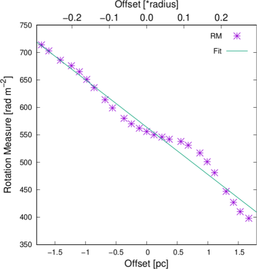
Figure 10: Rotation measure along the ridge of the bright shell in the north-east. The centre is at the peak in polarised intensity. The negative offset is to the lower left and the positive offset is to the upper right. The offset is given in pc (bottom) and in a fraction of the SNR’s radius (top). The green line indicates a linear fit to the gradient.

Kothes & Brown (2009) modelled radio polarisation observations of an SNR expanding inside a homogenous medium. We plotted our rotation measure along the bright polarised intensity ridge of the north-east shell in Fig. 10. The rotation measure observed from the SNR’s radio shell is dominated by the magnetic field in the nearby part of the SNR. In this nearby part, one side the magnetic field is coming towards us and the other is pointing away from us. If the ambient magnetic field is only in the plane of the sky (i.e., has no line-of-sight component) we should find a $RM$ of 0 in the centre, negative on one side and positive on the other. The centre $RM$ can be affected by the foreground $RM$ ($\sim$ +23 rad m^-2 as noted in Section 3.4), the angle between the plane of the sky, and the ambient magnetic field. In this case, we can determine that the ambient uniform magnetic field is pointing towards us, and is pointing from the bottom left to the top right as the $RM$ is positive but decreasing along the same direction. It only requires a small rotation angle to have all $RM$s in the positive or the negative on the shell. We fitted the gradient with a linear function, also shown in Fig. 10. The resulting $RM$ in the centre is $+531\pm 5$ rad m^-2, corrected for the foreground contribution of the MW. The contribution of the SMC is unclear as we stated in Section 3.4. At the bright ridge on the SNR’s shell, located at the inner edge, the line-of-sight through the emission region is the longest. With a radius of 5.8 pc and a compression ratio of 3.7, this line-of-sight should be 5.3 pc. In the shell of the SNR, synchrotron emitting and Faraday rotating plasmas are intermixed. Therefore, the synchrotron emission generated at the back of the SNR sees the entire $RM$ and the emission generated at the front sees no $RM$. If all the parameters, as synchrotron emissivity, magnetic field strength and angle, and electron density are approximately constant along the line of sight through the SNR shell and the polarised emission is Faraday thin, the $RM$ seen by a background source is twice the value observed (Burn, 1966). Using equation 3, with $RM=2\times 531$ rad m${}^{-2}=1062$ rad m^-2, $dl$ = 5.3 pc, and electron density $n_{e}$ = 14.8 cm^-3 for the post-shock gas (Vogt et al., 2017), the magnetic field strength of the uniform component inside the shell parallel to the line-of-sight is $B_{\parallel}$ = 16.7 $\mu$G.

We can assume the intrinsic percentage polarisation of the SNR’s synchrotron emission through the spectral index to be 71 per cent (Le Roux, 1961). In the shell of the SNR, where the synchrotron emitting and Faraday rotating plasmas are intermixed, a high rotation measure (as we measured) causes depolarisation even at such a high frequency. According to Sokoloff et al. (1998), the $RM$ value we found in the middle of the shell, would reduce the percentage polarisation from 71 per cent to 55.7 per cent. But, in the centre of the shell, we observe a 15 per cent linear polarisation. This additional depolarisation is caused by random fluctuations of the magnetic field (Burn, 1966). From this depolarisation, we estimate the ratio between the uniform and random components of the magnetic field. This high depolarisation here requires a random magnetic field component of 27.5 $\mu$G, using the above calculated 16.7 $\mu$G as the uniform component. In this case, we would have a total magnetic field in the shell of $\sim$44 $\mu$G. The uncertainty in magnetic field strength remains undetermined, primarily due to it being a combination of the uncertainties associated with the RM and electron density, with the electron density’s uncertainty being unquantified.

This of course only takes the line-of-sight component of the magnetic field into account. To achieve the magnetic field strengths estimated through equipartition, we require an angle of 38° between the plane of the sky and the ambient magnetic field for $\sim 65$ $\mu$G, containing a uniform magnetic field of 24.7 $\mu$G, after scaling 16.7 $\mu$G as given above. Correcting for compression, we can extrapolate a total ambient magnetic field strength of the uniform components to 5.1 $\mu$G. Here, we cannot simply apply the linear compression ratio of 3.7, as the magnetic field is not only compressed but also enhanced. The ‘magnetic field lines’ are frozen into the plasma of the expanding shell and therefore also stretched out around the perimeter of the SNR, which increases the magnetic energy (Whiteoak & Gardner, 1968). This leads to a combined compression and enhancement of 4.8.

3.6 Hi/CO morphology

The E0102 SNR region was mapped in Hi using ASKAP from Pingel et al. (2022); these velocity channel maps are shown in Fig. 11, with our 5500 MHz image overlaid. Hi emission is visible in the velocity range of $\sim$160–180 km s^-1. There appears to be a cavity-like structure forming near the location of E0102 in the velocity range 165.0–168.9 km s^-1(see Fig. 12, a). A large cloud is seen at $\sim$170–180 km s^-1 in the north at Dec $>-$72^∘02$\arcmin$, which then transitions to a cloud in the west at $\sim$160–175 km s^-1(RA $<$ 01^h04^m). Those emission regions are most likely connected at the velocities around E0102. The boundary of Hi appears along the radio shell, especially towards the south-west.

The Hi distribution in the velocity space has unique features. Fig. 12(b) shows the position–velocity ($p$–$v$) diagram of Hi. We found a cavity-like structure of Hi, whose size is roughly three times larger than the diameter of the SNR shell. We propose a possible scenario that the cavity-like structures in both the spatial distribution and $p$–$v$ diagram correspond to a wind-blown bubble that was formed by strong stellar winds from a high-mass progenitor of E0102 and is now partially interacting with an inner wall of the Hi cavity. The observational signature is similar to Hi studies of core-collapse SNRs in the SMC (DEM S5, Alsaberi et al. 2019b; RX J0046.5$-$7308, Sano et al. 2019b). However, more data are required to draw definitive conclusions regarding this scenario, in particular, further Hi observations at higher angular resolutions.

Multi–J CO observations could also give better insight into the nature of E0102. Fig. 13 shows the peak temperature map of the ¹²CO (J = 2–1) emission line obtained with ALMA (Tokuda et al., 2021). Although several CO clumps are detected within the field of view shown in Fig. 11, we find no dense CO clumps towards the radio continuum shell of E0102, suggesting it is interacting with only the Hi clouds.

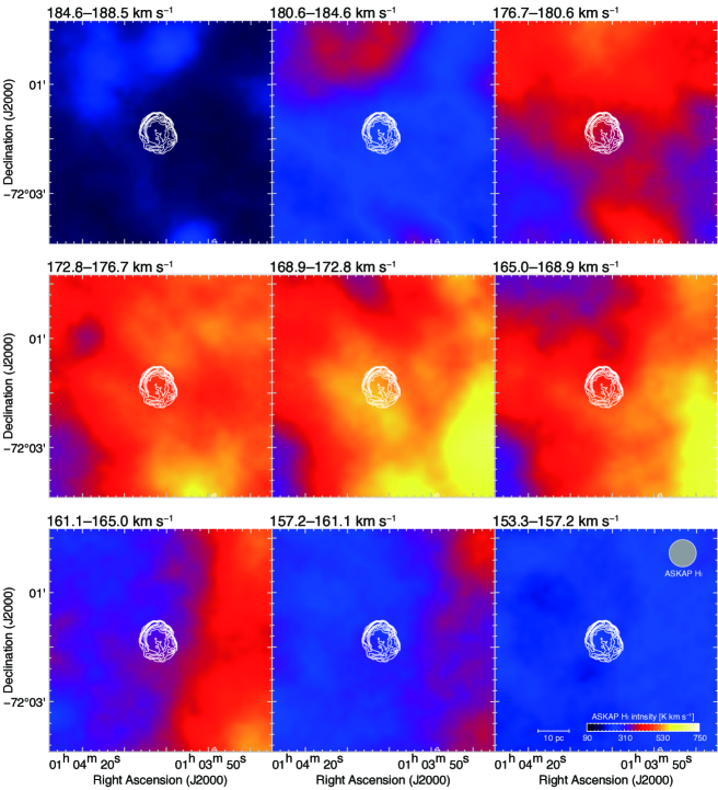
Figure 11: Velocity channel map of Hi towards E0102 obtained from the ASKAP (Pingel et al., 2022). Each panel shows the Hi intensity distribution integrated every 3.9 km s^-1 in a velocity range from 188.5 to 153.3 km s^-1. Our 5500 MHz ATCA image has been overlaid on top with contours levels as per Fig. 2. The grey circle and colour bar on the bottom right panel represent a synthesised beam of $30\times 30$ arcsec² and gradients of Hi in K km s^-1, respectively. A bar for physical size on the sky is shown.

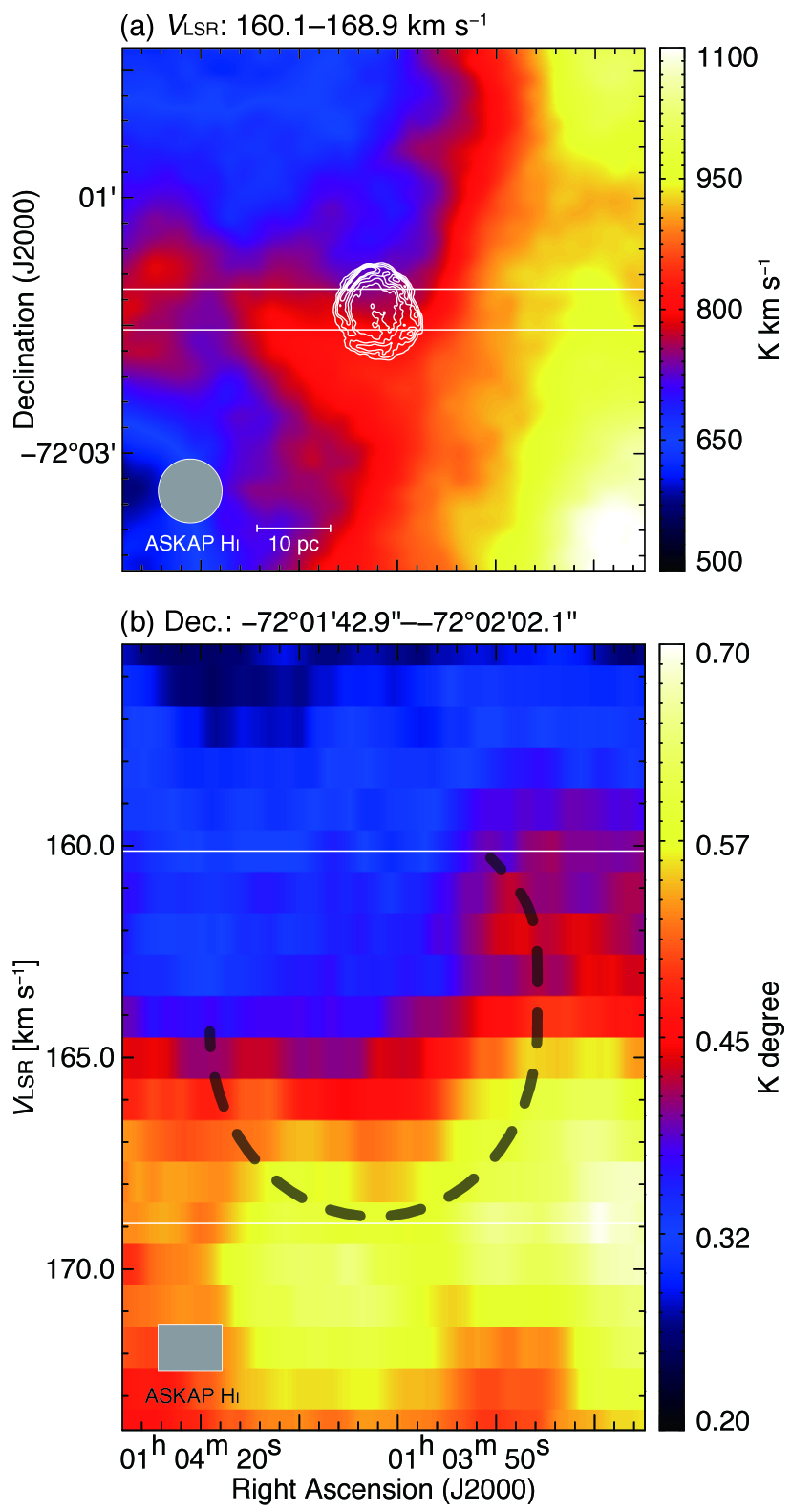
Figure 12: (a) Hi integrated velocity intensity map towards E0102, where the integration velocity range is from 160.1 to 168.9 km s^-1. Our 5500 MHz image is overlaid with intensity levels as per Fig. 2. (b) Position–velocity diagram of Hi with Declination $-72^{\circ}01^{\prime}42\aas@@fstack{\prime\prime}9$ to $-72^{\circ}02^{\prime}02\aas@@fstack{\prime\prime}1$. The dashed curve delineates a possible expanding gas motion (see text).

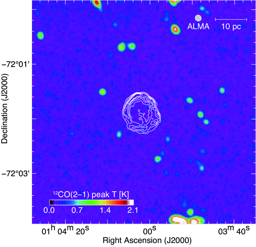
Figure 13: Peak temperature map of ¹²CO ($J$ = 2–1) line emission towards E0102 obtained from ALMA. Our ATCA 5500 MHz image is overlaid in contours, with levels as per Fig. 2. In the upper right-hand corner, the ALMA synthesised beam and a bar representing physical size on the sky is shown, while a colour bar at the bottom indicates CO gradients in K.

4 Discussion

Our new radio continuum and polarisation study of E0102 reveal typical characteristics of a young SNR. We found a low integrated linear polarisation which indicates a high degree of turbulence. The total radio-continuum spectrum is rather steep which is also found in other young SNRs (see Table 3) and we found areas of radial magnetic fields typically seen in younger remnants. In this section, we discuss our results in relation to E0102’s environment and magnetic field comparing them to other young SNRs.

4.1 The environment of E0102

Our study of Hi line emission surrounding E0102 (Section 3.6) reveals the possibility of a stellar wind bubble; a closer look at the structure of this SNR’s environment is therefore warranted. The measurements of Vogt et al. (2017) indicate a pre-shock density of $n_{0}\approx 4\pm 1$ cm^-3 ($n_{0}\approx 7.4\pm 1.5$ cm^-3) surrounding E0102, based on [Fe xiv] and [Fe xi] [O iii] measurements. This density, however, appears high given typical densities of about 0.02 cm^-3 (Weaver et al., 1977) in such wind-bubbles and would indicate that the SNR-shock has reached the ISM. Taking 7.4 cm^-3 as the pre-shock density and using $r_{\rm w}=56n_{0}^{-0.3}$ pc (McKee et al., 1984) to calculate the wind-bubble size, one finds $r_{\rm w}\geq 30$ pc, which is almost five times the radius of E0102. Further, the expansion rate derived by Vogt et al. (2017) differs strongly from the rate derived by Xi et al. (2019). A possible explanation is that Vogt et al. (2017) measured the downstream density and obtained an upstream density by assuming the canonical shock compression-ratio of $\approx 4$. In general, the [Fe xiv] and [Fe xi] emissions are not associated with the outer-most regions of E0102. Hence, the emission can be an imprint of a previous interaction of the SNR-blastwave with a dense structure in the progenitor’s wind, breaking the simple relation between up- and downstream density. Massive stars undergo different stages of evolution, and depending on their ZAMS-mass, winds get crushed by stronger winds of subsequent evolutionary stages. Shell-like features can emerge as a consequence and influence the following SNR evolution as shown for a massive progenitor with a crushed LBV-shell in Das et al. (2022). There is evidence that interaction with such a dense and asymmetric shell in the case of Cassiopeia A is responsible for the observed expansion dynamics of that remnant (Orlando et al., 2022).

Given the possible presence of a dense shell in the progenitor’s wind, it is likely that E0102 has already entered the Sedov-phase as suggested by Xi et al. (2019). However, the structure of wind-bubbles also featured a transition between the free-expanding wind, where $\rho\propto r^{-2}$, and a shocked wind with roughly constant density. Further detailed modelling of the apparently complex environment of E0102 is beyond the scope of this paper.

4.2 Comparison with other young SNRs

Insight into our results for E0102 is compared to the broader SNR population by listing properties (e.g. size, spectral index and polarisation) with other young SNRs ($\leq$1000 yrs) in the MW and LMC (Table 3).

4.2.1 Diameter

The diameter of SNRs from our selected sample varies from 0.4 pc for the youngest (1987 A; 36 yr) to $\sim$23 pc for the oldest (G266.2–1.2; 2400–5100 yr). Although N 132D and E0102 have similar ages ($\sim$2000 yr), N 132D is nearly twice the diameter. Perhaps this is related to the radio surface brightness at 1 GHz ($\Sigma_{\rm 1\,GHz}$ for N 132D is 27.9$\times 10^{-20}$ W m^-2 Hz^-1 sr^-1 (Bozzetto et al., 2017) versus 9.7$\times 10^{-20}$ W m^-2 Hz^-1 sr^-1 for E0102, see Table 3). Typically one would expect a remnant with a higher ambient density to be brighter (and smaller), but a higher explosion energy could cause a SNR to be larger and brighter at the same age. The diameters for bright LMC SNRs N 49 and N 63A are $\sim$18 pc which is comparable to the diameter of E0102. Selected type Ia (thermonuclear) SNRs (N 103B, J0509–6731, LHG 26, and Kepler) are slightly younger, which may account for their smaller diameters (7–8 pc). The youngest SNRs from our sample (Cas A, G1.9+0.3 and Tycho) display smaller diameters, $\sim$5 pc, as they have not yet expanded as far as their older counterparts. Various factors such as the composition of the ambient medium, explosion energy, and age all play an important role in the diameter of SNRs.

4.2.2 Spectral Index

E0102 has a spectral index ($\alpha$) within the range of SNRs listed in Table 3, although there is a slight trend for older SNRs to have shallower values (Bozzetto et al., 2017; Filipović et al., 2022). The spectral index for E0102, $\alpha=-0.61\pm 0.01$, is similar to that of N 132D, Kepler, and Tycho (see values and references in Table 3 which suggest a similar evolutionary phase). Other radio spectral indices vary from –0.81 in the youngest Galactic SNR (G1.9+0.3) to –0.3 in the oldest (G266.2–1.2) as expected (see e.g. Urošević, 2014, for review).

4.2.3 Polarisation and Magnetic Field

The mean fractional polarisation of SNRs varies as a function of age. Young SNR fractional polarisation can be as high as $\sim$20 per cent, while older ones may have twice that value (Dickel & Jones, 1990) . Values of well-studied SNRs within the LMC, as shown in Table 3, vary from 3 to $\sim$26 per cent . Since E0102 has fractional polarisations of $7\pm 1$ and $12\pm 2$  per cent (at 5500 and 9000 MHz, respectively), we suggest its age and evolutionary phase (and possibly environmental conditions) are typical of this population.

MW SNRs also show disparity in values of fractional polarisation ($P$). $P$ for the youngest Galactic SNR (G1.9+0.3) is very low (6 per cent) compared with Tycho (20–30 per cent) and SN 1006 (17 per cent). This diversity of $P$ may be due to the difference in ambient density and SNR age, as well as observational effects due to various radio telescope configurations. Fractional polarisation significantly changes with frequency because of Faraday rotation, which affects lower frequencies much more than higher frequencies. These issues make $P$ comparison difficult.

We estimate the line-of-sight magnetic field strength of E0102 is $\sim 44$ $\mu$G, which is higher than the value of the same age SNR N 132D (Table 3). However, the equipartition field of E0102 is $65\pm 5$ $\mu$G, similar to the N 49 value of 91.2 $\mu$G. Interestingly, Cas A, an oxygen-rich SNR in the MW, shows a high magnetic field strength value of 780 $\mu$G (Arias et al., 2018) due to the low value of $P$, indicative of a highly turbulent magnetic field (Vink, 2020). Similar behaviour can be seen in other MW SNRs (see Table 3).

4.2.4 Surface Brightness and Luminosity

The surface brightness ($\Sigma_{\rm 1\,GHz}$) for all SNRs used here for comparison shows, as expected, a variety of intensities. While, SNR 1987A displays a high $\Sigma_{\rm 1\,GHz}$ of $13700\times 10^{-20}$ W m^-2 Hz^-1 sr^-1 as it is the youngest Local Group SNR, recently discovered intergalactic SNR J0624–6948 is barely detectable with a $\Sigma_{\rm 1\,GHz}$ of $0.0154\times 10^{-20}$ W m^-2 Hz^-1 sr^-1. We note Cas A also has quite a high value $\Sigma_{\rm 1\,GHz}$ of $1145.27\times 10^{-20}$ W m^-2 Hz^-1 sr^-1 (Table 3).

Comparing a previous $\Sigma$–D diagram (Urošević, 2022, 2020; Pavlović et al., 2018, their fig. 3) and our values, D = $\sim$13 pc and $\Sigma_{\rm 1\,GHz}=9.17\times 10^{-20}$ W m^-2 Hz^-1 sr^-1 for E0102 (see Table 3), E0102 is in the middle of their $\Sigma$–D diagram. This is consistent with a Sedov phase having a dense ambient density of $n_{\rm H}=0.5$ cm^-3.

Finally, we note that E0102 has a $L_{\rm 1\,GHz}$ of 1.4$\times 10^{17}$ W Hz^-1, which is less than the values of some LMC SNRs (N 49 and N 63A), while similar age N 132D shows a much higher value (15.7$\times 10^{17}$ W Hz^-1). The MW SNRs have less $L_{\rm 1\,GHz}$ than E0102, apart from Cas A which shows a high value of 36.1$\times 10^{17}$ W Hz^-1. Therefore, E0102 has a $L_{\rm 1\,GHz}$ less than many young LMC SNRs but greater than most young SNRs in the MW.

Table 3: Comparison of E0102 with young SNRs ($\leq$1000 yrs) in the MW and LMC. SN type is denoted by CC – Core-Collapse, and TN – Thermonuclear (type Ia). Magnetic field strength for the molecular cloud associated with the SNR is marked with an asterisk (^∗) and magnetic field strength estimation using equipartition is marked with an double asterisk (^∗∗).

Name	Host	SN	Age	Diameter	Spectral Index	Avg. $P$	$P_{\nu}$	Mag. Field	$\Sigma_{\rm 1\,GHz}(\times 10^{-20})$
	Galaxy	Type	(yr)	(pc)	($\alpha$)	(%)	(MHz)	($\mu$G)	(W m-2 Hz-1 sr-1)
E0102	SMC	CC	$\sim 1738^{1}$	$\sim 13$	$-0.61\pm 0.01$	$7\pm 1/12\pm 2$	$5500/9000$	$65\pm 5^{**}$	$9.17$
J0624–6948	LMC	TN2	$2200^{2}$	$47.5^{2}$	$-0.54\pm 0.08^{2}$	$\leq 9^{2}$	$5500^{2}$	—	$0.0154^{2}$
N 49	LMC	CC	$\sim 4800^{3}$	$18.2^{4}$	$-0.56\pm 0.03^{4}$	$4.8^{5}$	$8640^{5}$	$91.2^{**}$	$16^{4}$
N 132D	LMC	CC	$\sim 2500^{6}$	$24.5^{4}$	$-0.65\pm 0.04^{4}$	$4^{7}$	$4790^{7}$	$2.1^{7}$	$27.9^{4}$
N 63A	LMC	CC	$3500\pm 1500^{8}$	$17.8^{4}$	$-0.740\pm 0.002^{8}$	$5\pm 1^{9}$	$5500^{9}$	$80-180^{9*}$	$18.7^{4}$
1987 A	LMC	CC	$34$	$0.4^{4}$	$-0.8^{10}$	$2.7\pm 0.2^{11}$	$22000^{11}$	$\sim 28^{11}$	$13700^{4}$
N 103B	LMC	TN	$380-860^{12}$	$6.8^{4}$	$\sim-0.75^{13}$	$8\pm 1^{13}$	$5500^{13}$	$0.03-82.1^{13}$	$60^{13}$
J0509–6731	LMC	TN	$\sim 310^{14}$	$7.4^{15}$	$-0.73^{16}$	$\sim 26^{16}$	$5500^{15}$	$\sim 128^{15**}$	$5.72^{4}$
LHG 26	LMC	TN	$\sim 600^{16}$	$8.3^{16}$	$\sim-0.54^{17}$	$\sim 8^{17}$	$5500^{17}$	$\sim 171^{17**}$	$6.09^{4}$
Cas A	MW	CC	$325^{18}$	$\sim 5^{19}$	$-0.77^{20}$	$4.5^{21}$	$19000^{21}$	$780^{19}$	$1145.27^{22}$
G1.9+0.3	MW	CC23	$\sim 120^{24}$	$4^{25}$	$-0.81\pm 0.02^{23}$	$6^{26}$	$5500^{26}$	$\sim 273^{26**}$	$6.7^{23}$
G266.2–1.2	MW	CC	$2400-5100^{27}$	$23.60\pm 0.06^{28}$	$\sim-0.3^{28}$	—	—	$6-10^{29}$	$0.05^{22}$
Tycho	MW	TN	$451^{30}$	$3.5-7.2^{30}$	$-0.58^{31}$	$20-30^{32}$	$4872^{32}$	$50-400^{33}$	$13.17^{22}$
SN1006	MW	TN	$1017^{34}$	$\sim 19^{34}$	$-0.6^{31}$	$\sim 17^{35}$	$1400^{35}$	$30-40^{36}$	$0.32^{22}$
Kepler	MW	TN	$419^{37}$	$8.18^{37}$	$-0.64^{31}$	$\sim 6^{38}$	$4835^{38}$	$\sim 414^{39**}$	$31.78^{22}$
G11.2$-$0.3	MW	CC	$1636^{40}{\dagger}$	$6.0$	$-0.56^{41}$	$\sim 2^{42}$	$32000^{42}$	—	$20.7^{31}$
G29.7–0.3	MW	CC	$\sim 480^{43}$	$5.0^{43}$	$-0.63\pm 0.02^{44}$	$\leq 1^{45}$	$2695^{45}$	—	$16.7^{31}$

• References: (1) Banovetz et al. (2021), (2) Filipović et al. (2022), (3) Park et al. (2012), (4) Bozzetto et al. (2017), (5) Dickel & Milne (1998), (6) Law et al. (2020), (7) Dickel & Milne (1995), (8) Warren et al. (2003), (9) Sano et al. (2019a), (10) Zanardo et al. (2013), (11) Zanardo et al. (2018), (12) Rest et al. (2005), (13) Alsaberi et al. (2019a), (14) Roper et al. (2018), (15) Bozzetto et al. (2014), (16) Borkowski et al. (2006), (17) Bozzetto et al. (2012), (18) Fesen et al. (2006), (19) Arias et al. (2018), (20) DeLaney et al. (2014), (21) Mayer & Hollinger (1968), (22) Vukotić et al. (2019), (23) Luken et al. (2020), (24) Pavlović (2017), (25) Reynolds et al. (2008), (26) De Horta et al. (2014), (27) Allen et al. (2015), (28) Maxted et al. (2018), (29) Kishishita et al. (2013), (30) Hughes (2000), (31) Green (2014), (32) Dickel et al. (1991), (33) Tran et al. (2015), (34) Winkler et al. (2003), (35) Reynoso et al. (2013), (36) Vink (2006), (37) Patnaude et al. (2012), (38) DeLaney et al. (2002), (39) Arbutina et al. (2012), (40) Clark & Stephenson (1977), (41) Tam et al. (2002), (42) Kothes & Reich (2001), (43) Reynolds et al. (2018), (44) Sun et al. (2011), (45) Duncan et al. (1999).
  †Note that Zhou et al. (2018) argues that SNR G7.7–3.7 is more likely SN from 386CE.

5 Conclusions

SNR E0102 is a young SNR located in the SMC with properties including spectral index and luminosity consistent with young SNRs in the MW and LMC. Our new radio continuum images of E0102 show a ring morphology and bridge-like structure seen in both optical and X-ray images. Our new images also show a central feature that lacks any significant polarisation towards it suggesting that the origin is not a PWN. We find that the remnant’s radio emission extends beyond its X-ray emission tracing a forward and reverse shock with [Fe XIV] emission sandwiched between possibly representing denser ionized clumps. The remnant shows polarised regions in its shell and it was possible to obtain a rotation measure and estimate its magnetic field. Comparison with theoretical intrinsic magnetic field estimates and location on a $\Sigma-D$ diagram of comparable SNRs are constant with it in or entering its Sadov phase with a high ambient density.

Data Availability

The data that support the plots/images within this paper and other findings of this study are available from the corresponding author upon reasonable request. The ASKAP data used in this article are available through the CSIRO ASKAP Science Data Archive (CASDA) and ATCA data via the Australia Telescope Online Archive (ATOA).

Please note: Oxford University Press is not responsible for the content or functionality of any supporting materials supplied by the authors. Any queries (other than missing material) should be directed to the corresponding author for the article.

¹Western Sydney University, Locked Bag 1797, Penrith, NSW, 2751, Australia
²CSIRO Astronomy and Space Sciences, Australia Telescope National Facility, PO Box 76, Epping, NSW 1710, Australia
³Faculty of Engineering, Gifu University, 1-1 Yanagido, Gifu 501-1193, Japan
⁴National Astronomical Observatory of Japan, Mitaka, Tokyo 181-8588, Japan
⁵Dominion Radio Astrophysical Observatory, Herzberg Astronomy and Astrophysics, National Research Council Canada, PO Box 248, Penticton BC V2A 6J9, Canada
⁶Dublin Institute for Advanced Studies, Astronomy & Astrophysics Section, 31 Fitzwilliam Place, D02 XF86 Dublin 2, Ireland
⁷Dr. Karl Remeis Observatory, Erlangen Centre for Astroparticle Physics, Friedrich-Alexander University Erlangen-Nürnberg, Sternwartstr. 7, 96049 Bamberg, Germany
⁸Max-Planck-Institut für extraterrestrische Physik, Gießenbachstraße 1, 85748 Garching, Germany
⁹School of Cosmic Physics, Dublin Institute for Advanced Studies, 31 Fitzwillam Place, Dublin 2, Ireland
¹⁰Department of Physics and Astronomy, University of Calgary, University of Calgary, Calgary, Alberta, T2N 1N4, Canada
¹¹Observatoire Astronomique de Strasbourg, Université de Strasbourg, CNRS, 11 rue de l’Université, F-67000 Strasbourg, France
¹²European Southern Observatory, Alonso de Córdova 3107, Vitacura 763 0355, Santiago, Chile
¹³Joint ALMA Observatory, Alonso de Córdova 3107, Vitacura 763 0355, Santiago, Chile
¹⁴School of Physical Sciences, The University of Adelaide, Adelaide 5005, Australia
¹⁵School of Science, University of New South Wales, Australian Defence Force Academy, Canberra, ACT 2600, Australia
¹⁶Department of Earth and Planetary Sciences, Faculty of Sciences, Kyushu University, Nishi-ku, Fukuoka 819-0395, Japan
¹⁷National Astronomical Observatory of Japan, National Institutes of Natural Sciences, 2-21-1 Osawa, Mitaka, Tokyo 181-8588, Japan
¹⁸Department of Physics, Graduate School of Science, Osaka Metropolitan University, 1-1 Gakuen-cho, Naka-ku, Sakai, Osaka 599-8531, Japan
¹⁹Department of Astronomy, Faculty of Mathematics, University of Belgrade, Studentski trg 16, 11000 Belgrade, Serbia
²⁰Isaac Newton Institute of Chile, Yugoslavia Branch
²¹Lennard-Jones Laboratories, Keele University, Staffordshire ST5 5BG, UK
²²Federal Office of Meteorology and Climatology - MeteoSwiss, Chemin de l’Aérologie 1, 1530 Payerne, Switzerland

References

- Alan et al. (2019) Alan N., Park S., Bilir S., 2019, ApJ, 873, 53
- Allen et al. (2015) Allen G. E., Chow K., DeLaney T., Filipović M. D., Houck J. C., Pannuti T. G., Stage M. D., 2015, ApJ, 798, 82
- Alsaberi et al. (2019a) Alsaberi R. Z. E., et al., 2019a, Ap&SS, 364, 204
- Alsaberi et al. (2019b) Alsaberi R. Z. E., et al., 2019b, MNRAS, 486, 2507
- Amy & Ball (1993) Amy S. W., Ball L., 1993, ApJ, 411, 761
- Arbutina et al. (2012) Arbutina B., Urošević D., Andjelić M. M., Pavlović M. Z., Vukotić B., 2012, ApJ, 746, 79
- Arbutina et al. (2013) Arbutina B., Urošević D., Vučetić M. M., Pavlović M. Z., Vukotić B., 2013, ApJ, 777, 31
- Arias et al. (2018) Arias M., et al., 2018, A&A, 612, A110
- Banovetz et al. (2021) Banovetz J., et al., 2021, ApJ, 912, 33
- Blair et al. (2000) Blair W. P., et al., 2000, ApJ, 537, 667
- Borkowski et al. (2006) Borkowski K. J., et al., 2006, ApJ, 642, L141
- Bozzetto et al. (2012) Bozzetto L. M., Filipovic M. D., Urosevic D., Crawford E. J., 2012, Serbian Astronomical Journal, 185, 25
- Bozzetto et al. (2014) Bozzetto L. M., Filipović M. D., Urošević D., Kothes R., Crawford E. J., 2014, MNRAS, 440, 3220
- Bozzetto et al. (2017) Bozzetto L. M., et al., 2017, ApJS, 230, 2
- Bozzetto et al. (2023) Bozzetto L. M., et al., 2023, MNRAS, 518, 2574
- Brantseg et al. (2014) Brantseg T., McEntaffer R. L., Bozzetto L. M., Filipovic M., Grieves N., 2014, ApJ, 780, 50
- Brentjens & de Bruyn (2005) Brentjens M. A., de Bruyn A. G., 2005, A&A, 441, 1217
- Burn (1966) Burn B. J., 1966, MNRAS, 133, 67
- Clark & Stephenson (1977) Clark D. H., Stephenson F. R., 1977, The historical supernovae. Pergamon Press, doi:https://doi.org/10.1016/C2013-0-10100-6
- Clarke et al. (1976) Clarke J. N., Little A. G., Mills B. Y., 1976, Australian Journal of Physics Astrophysical Supplement, 40, 1
- Collischon et al. (2021) Collischon C., Sasaki M., Mecke K., Points S. D., Klatt M. A., 2021, A&A, 653, A16
- Cortes et al. (2020) Cortes P. C., et al., 2020, ALMA Technical Handbook,ALMA Doc. 8.4, ver. 1.0, 2020, ALMA Technical Handbook,ALMA Doc. 8.4, ver. 1.0 ISBN 978-3-923524-66-2
- Crawford et al. (2008) Crawford E. J., Filipovic M. D., de Horta A. Y., Stootman F. H., Payne J. L., 2008, Serbian Astronomical Journal, 177, 61
- Das et al. (2022) Das S., Brose R., Meyer D. M. A., Pohl M., Sushch I., Plotko P., 2022, A&A, 661, A128
- De Horta et al. (2014) De Horta A. Y., et al., 2014, Serbian Astronomical Journal, 189, 41
- DeLaney et al. (2002) DeLaney T., Koralesky B., Rudnick L., Dickel J. R., 2002, ApJ, 580, 914
- DeLaney et al. (2014) DeLaney T., Kassim N. E., Rudnick L., Perley R. A., 2014, ApJ, 785, 7
- Dickel & Jones (1990) Dickel J. R., Jones E. M., 1990, in Beck R., Kronberg P. P., Wielebinski R., eds, International Astronomical Union (IAU) Series Vol. 140, Galactic and Intergalactic Magnetic Fields. p. 81
- Dickel & Milne (1995) Dickel J. R., Milne D. K., 1995, AJ, 109, 200
- Dickel & Milne (1998) Dickel J. R., Milne D. K., 1998, AJ, 115, 1057
- Dickel et al. (1991) Dickel J. R., van Breugel W. J. M., Strom R. G., 1991, AJ, 101, 2151
- Dopita et al. (1981) Dopita M. A., Tuohy I. R., Mathewson D. S., 1981, ApJ, 248, L105
- Duncan et al. (1999) Duncan A. R., Reich P., Reich W., Fürst E., 1999, A&A, 350, 447
- Fesen et al. (2006) Fesen R. A., et al., 2006, ApJ, 645, 283
- Filipović & Tothill (2021) Filipović M. D., Tothill N. F. H., 2021, Principles of Multimessenger Astronomy. AAS-IOP astronomy, Institute of Physics Publishing, doi:10.1088/2514-3433/ac087e
- Filipović et al. (2002) Filipović M. D., Bohlsen T., Reid W., Staveley-Smith L., Jones P. A., Nohejl K., Goldstein G., 2002, MNRAS, 335, 1085
- Filipović et al. (2022) Filipović M. D., et al., 2022, MNRAS, 512, 265
- Findlay (1966) Findlay J. W., 1966, ARA&A, 4, 77
- Finkelstein et al. (2006) Finkelstein S. L., et al., 2006, ApJ, 641, 919
- Flanagan et al. (2004) Flanagan K. A., Canizares C. R., Dewey D., Houck J. C., Fredericks A. C., Schattenburg M. L., Markert T. H., Davis D. S., 2004, ApJ, 605, 230
- For et al. (2018) For B. Q., et al., 2018, MNRAS, 480, 2743
- Fruscione et al. (2006) Fruscione A., et al., 2006, in Silva D. R., Doxsey R. E., eds, Society of Photo-Optical Instrumentation Engineers (SPIE) Conference Series Vol. 6270, Society of Photo-Optical Instrumentation Engineers (SPIE) Conference Series. p. 62701V, doi:10.1117/12.671760
- Gaetz et al. (2000) Gaetz T. J., Butt Y. M., Edgar R. J., Eriksen K. A., Plucinsky P. P., Schlegel E. M., Smith R. K., 2000, ApJ, 534, L47
- Gooch (1995) Gooch R., 1995, in Shaw R. A., Payne H. E., Hayes J. J. E., eds, Astronomical Society of the Pacific Conference Series Vol. 77, Astronomical Data Analysis Software and Systems IV. p. 144
- Graczyk et al. (2020) Graczyk D., et al., 2020, ApJ, 904, 13
- Graessle et al. (2007) Graessle D. E., Evans I. N., Glotfelty K., He X. H., Evans J. D., Rots A. H., Fabbiano G., Brissenden R. J., 2007, Chandra News, 14, 33
- Green (2014) Green D. A., 2014, Bulletin of the Astronomical Society of India, 42, 47
- Haberl et al. (2012) Haberl F., et al., 2012, A&A, 543, A154
- Hancock et al. (2018) Hancock P. J., Trott C. M., Hurley-Walker N., 2018, PASA, 35, e011
- Higgs et al. (1997) Higgs L. A., Hoffmann A. P., Willis A. G., 1997, in Hunt G., Payne H., eds, Astronomical Society of the Pacific Conference Series Vol. 125, Astronomical Data Analysis Software and Systems VI. p. 58
- Hilditch et al. (2005) Hilditch R. W., Howarth I. D., Harries T. J., 2005, MNRAS, 357, 304
- Hughes (2000) Hughes J. P., 2000, ApJ, 545, L53
- Hurley-Walker et al. (2021) Hurley-Walker N., Payne J. L., Filipović M. D., Tothill N., 2021, in Filipović M. D., Tothill N. F. H., eds, 2514-3433, Multimessenger Astronomy in Practice. IOP Publishing, pp 2–1, doi:10.1088/2514-3433/ac2256ch2
- Joseph et al. (2019) Joseph T. D., et al., 2019, MNRAS, 490, 1202
- Joye & Mandel (2003) Joye W. A., Mandel E., 2003, in Payne H. E., Jedrzejewski R. I., Hook R. N., eds, Astronomical Society of the Pacific Conference Series Vol. 295, Astronomical Data Analysis Software and Systems XII. p. 489
- Jun & Norman (1996) Jun B.-I., Norman M. L., 1996, ApJ, 465, 800
- Kishishita et al. (2013) Kishishita T., Hiraga J., Uchiyama Y., 2013, A&A, 551, A132
- Kothes & Brown (2009) Kothes R., Brown J.-A., 2009, in Strassmeier K. G., Kosovichev A. G., Beckman J. E., eds, International Astronomical Union (IAU) Series Vol. 259, Cosmic Magnetic Fields: From Planets, to Stars and Galaxies. pp 75–80 (arXiv:0812.3392), doi:10.1017/S1743921309030087
- Kothes & Reich (2001) Kothes R., Reich W., 2001, A&A, 372, 627
- Law et al. (2020) Law C. J., et al., 2020, ApJ, 894, 73
- Le Roux (1961) Le Roux E., 1961, Annales d’Astrophysique, 24, 71
- Livingston et al. (2022) Livingston J. D., McClure-Griffiths N. M., Mao S. A., Ma Y. K., Gaensler B. M., Heald G., Seta A., 2022, MNRAS, 510, 260
- Luken et al. (2020) Luken K. J., et al., 2020, MNRAS, 492, 2606
- Maggi et al. (2019) Maggi P., et al., 2019, A&A, 631, A127
- Mao et al. (2008) Mao S. A., Gaensler B. M., Stanimirović S., Haverkorn M., McClure-Griffiths N. M., Staveley-Smith L., Dickey J. M., 2008, ApJ, 688, 1029
- Maxted et al. (2018) Maxted N. I., et al., 2018, ApJ, 866, 76
- Mayer & Hollinger (1968) Mayer C. H., Hollinger J. P., 1968, ApJ, 151, 53
- McKee et al. (1984) McKee C. F., van Buren D., Lazareff B., 1984, ApJ, 278, L115
- McMullin et al. (2007) McMullin J. P., Waters B., Schiebel D., Young W., Golap K., 2007, in Shaw R. A., Hill F., Bell D. J., eds, Astronomical Society of the Pacific Conference Series Vol. 376, Astronomical Data Analysis Software and Systems XVI. p. 127
- Milne (1995) Milne D. K., 1995, MNRAS, 277, 1435
- Orlando et al. (2022) Orlando S., et al., 2022, A&A, 666, A2
- Otsuka et al. (2010) Otsuka M., et al., 2010, A&A, 518, L139
- Park et al. (2012) Park S., Hughes J. P., Slane P. O., Burrows D. N., Lee J.-J., Mori K., 2012, ApJ, 748, 117
- Patnaude et al. (2012) Patnaude D. J., Badenes C., Park S., Laming J. M., 2012, ApJ, 756, 6
- Pavlović (2017) Pavlović M. Z., 2017, MNRAS, 468, 1616
- Pavlović et al. (2018) Pavlović M. Z., Urošević D., Arbutina B., Orlando S., Maxted N., Filipović M. D., 2018, ApJ, 852, 84
- Pingel et al. (2022) Pingel N. M., et al., 2022, Publ. Astron. Soc. Australia, 39, e005
- Rest et al. (2005) Rest A., et al., 2005, Nature, 438, 1132
- Reynolds et al. (2008) Reynolds S. P., Borkowski K. J., Green D. A., Hwang U., Harrus I., Petre R., 2008, ApJ, 680, L41
- Reynolds et al. (2018) Reynolds S. P., Borkowski K. J., Gwynne P. H., 2018, ApJ, 856, 133
- Reynoso et al. (2013) Reynoso E. M., Hughes J. P., Moffett D. A., 2013, AJ, 145, 104
- Roper et al. (2018) Roper Q., et al., 2018, MNRAS, 479, 1800
- Sano et al. (2019a) Sano H., et al., 2019a, ApJ, 873, 40
- Sano et al. (2019b) Sano H., et al., 2019b, ApJ, 881, 85
- Sasaki et al. (2006) Sasaki M., Gaetz T. J., Blair W. P., Edgar R. J., Morse J. A., Plucinsky P. P., Smith R. K., 2006, ApJ, 642, 260
- Sault et al. (1995) Sault R. J., Teuben P. J., Wright M. C. H., 1995, in Shaw R. A., Payne H. E., Hayes J. J. E., eds, Astronomical Society of the Pacific Conference Series Vol. 77, Astronomical Data Analysis Software and Systems IV. p. 433 (arXiv:astro-ph/0612759)
- Sedov (1959) Sedov L. I., 1959, Similarity and Dimensional Methods in Mechanics. Academic Press, doi:https://doi.org/10.1016/C2013-0-08173-X
- Seward & Mitchell (1981) Seward F. D., Mitchell M., 1981, ApJ, 243, 736
- Sokoloff et al. (1998) Sokoloff D. D., Bykov A. A., Shukurov A., Berkhuijsen E. M., Beck R., Poezd A. D., 1998, MNRAS, 299, 189
- Stanimirović et al. (2005) Stanimirović S., Bolatto A. D., Sandstrom K., Leroy A. K., Simon J. D., Gaensler B. M., Shah R. Y., Jackson J. M., 2005, ApJ, 632, L103
- Stupar et al. (2005) Stupar M., Filipović M. D., Jones P. A., Parker Q. A., 2005, Advances in Space Research, 35, 1047
- Sun et al. (2011) Sun X. H., Reich P., Reich W., Xiao L., Gao X. Y., Han J. L., 2011, A&A, 536, A83
- Tam et al. (2002) Tam C., Roberts M. S. E., Kaspi V. M., 2002, ApJ, 572, 202
- Tokuda et al. (2021) Tokuda K., et al., 2021, ApJ, 922, 171
- Tran et al. (2015) Tran A., Williams B. J., Petre R., Ressler S. M., Reynolds S. P., 2015, ApJ, 812, 101
- Turtle et al. (1998) Turtle A. J., Ye T., Amy S. W., Nicholls J., 1998, Publ. Astron. Soc. Australia, 15, 280
- Urošević (2014) Urošević D., 2014, Ap&SS, 354, 541
- Urošević (2020) Urošević D., 2020, Nature Astronomy, 4, 910
- Urošević (2022) Urošević D., 2022, PASP, 134, 061001
- Urošević et al. (2018) Urošević D., Pavlović M. Z., Arbutina B., 2018, ApJ, 855, 59
- Vink (2006) Vink J., 2006, in Wilson A., ed., ESA Special Publication Vol. 604, The X-ray Universe 2005. p. 319 (arXiv:astro-ph/0601131)
- Vink (2020) Vink J., 2020, Physics and evolution of supernova remnants. Astronomy and astrophysics library, Springer, Cham, Switzerland
- Vogt et al. (2017) Vogt F. P. A., Seitenzahl I. R., Dopita M. A., Ghavamian P., 2017, A&A, 602, L4
- Vukotić et al. (2019) Vukotić B., Ćiprijanović A., Vučetić M. M., Onić D., Urošević D., 2019, Serbian Astronomical Journal, 199, 23
- Warren et al. (2003) Warren J. S., Hughes J. P., Slane P. O., 2003, ApJ, 583, 260
- Weaver et al. (1977) Weaver R., McCray R., Castor J., Shapiro P., Moore R., 1977, ApJ, 218, 377
- Whiteoak & Gardner (1968) Whiteoak J. B., Gardner F. F., 1968, ApJ, 154, 807
- Winkler et al. (2003) Winkler P. F., Gupta G., Long K. S., 2003, ApJ, 585, 324
- Xi et al. (2019) Xi L., Gaetz T. J., Plucinsky P. P., Hughes J. P., Patnaude D. J., 2019, The Astrophysical Journal, 874, 14
- Zanardo et al. (2013) Zanardo G., Staveley-Smith L., Ng C. Y., Gaensler B. M., Potter T. M., Manchester R. N., Tzioumis A. K., 2013, ApJ, 767, 98
- Zanardo et al. (2018) Zanardo G., Staveley-Smith L., Gaensler B. M., Indebetouw R., Ng C. Y., Matsuura M., Tzioumis A. K., 2018, ApJ, 861, L9
- Zhou et al. (2018) Zhou P., Vink J., Li G., Domček V., 2018, ApJ, 865, L6
- Zirakashvili et al. (2014) Zirakashvili V. N., Aharonian F. A., Yang R., Oña-Wilhelmi E., Tuffs R. J., 2014, ApJ, 785, 130
- van den Bergh (1988) van den Bergh S., 1988, ApJ, 327, 156