Design considerations for the optimization of $\lambda$-SQUIDs

Abstract

Cryogenic microcalorimeters are key tools for high-resolution X-ray spectroscopy due to their excellent energy resolution and quantum efficiency close to $100\text{\,}\mathrm{\char 37\relax}$. Multiple types of microcalorimeters exist, some of which have already proven outstanding performance. Nevertheless, they can’t yet compete with cutting-edge grating or crystal spectrometers. For this reason, novel microcalorimeter concepts are continuously developed. One such concept is based on the strong temperature dependence of the magnetic penetration depth of a superconductor operated close to its transition temperature. This so-called $\lambda$-SQUID provides an in-situ tunable gain and promises to reach sub-eV energy resolution. Here, we present some design considerations with respect to the optimization of such a detector that are derived by analytic means. We particularly show that for this detector concept the heat capacity of the sensor should match the heat capacity of the absorber.

1 Introduction

Cryogenic microcalorimeters such as superconducting transition-edge sensors (TESs) [1, 2] or metallic magnetic calorimeters (MMCs) [3, 4] have proven to be outstanding tools for measuring the energy of X-ray photons with unprecedented precision. They rely on sensing the change in temperature of an X-ray absorber upon photon absorption using an extremely sensitive thermometer that is based either on a superconducting (TES) or paramagnetic (MMC) sensor material. Due to their unique combination of excellent energy resolution and quantum efficiency close to $100\text{\,}\mathrm{\char 37\relax}$, they offer significant advantages as compared to state-of-the-art grating or crystal X-ray spectrometers [5]. Their quantum efficiency significantly relaxes the requirements on X-ray beam intensity, which especially benefits measurements on strongly diluted or radiation sensitive samples [6, 7]. Moreover, they cover the entire tender X-ray range [5] that is hardly accessible with both, grating and crystal spectrometers.

State-of-the-art TES- and MMC-based X-ray detectors achieve an energy resolution (FWHM) of $0.72\,\mathrm{eV}$ for $1.5\,\mathrm{keV}$ photons [8] and of $1.25\,\mathrm{eV}$ for $5.9\,\mathrm{keV}$ photons [9] at near-unity quantum efficiency. However, despite of various ongoing developments, all targeting to improve the performance of these microcalorimeters, an energy resolution as low as of $100\,\mathrm{meV}$, required for investigating vibrations or $d$-$d$-excitations in soft X-ray spectroscopy or resonant inelastic X-ray scattering, has yet to be demonstrated. Against this background, we have recently proposed a novel type of microcalorimeter, called $\lambda$-SQUID, that promises to provide the required energy resolution [10].

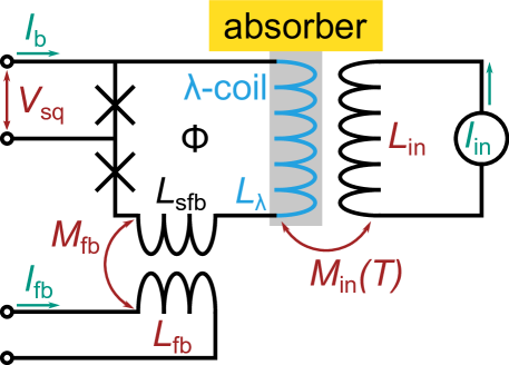
Figure 1: Simplified equivalent circuit diagram of a $\lambda$-SQUID. Inductors depicted in black are made from a superconductor with critical temperature $T_{\mathrm{c}}$. The $\lambda$-coil displayed in blue is made from a different superconductor with critical temperature $T_{\mathrm{c,\lambda}}\ll T_{\mathrm{c}}$, and is in strong thermal contact with the absorber. The device is operated at temperature $T_{0}\lessapprox T_{\mathrm{c,\lambda}}$. A constant current $I_{\mathrm{in}}$ is injected into an input coil with inductance $L_{\mathrm{in}}$ and causes a temperature dependent magnetic flux within the SQUID loop via the a temperature dependent mutual inductance $M_{\mathrm{in}}(T)$.

Fig. 1 shows a simplified equivalent circuit diagram of a $\lambda$-SQUID. Similar to a conventional dc-SQUID, it consists of a superconducting loop interrupted by two Josephson tunnel junctions, each with critical current $I_{\mathrm{c}}$, capacitance $C_{\mathrm{JJ}}$ and normal state resistance $R$. The superconducting loop is divided into two parts, i.e. a section $L_{\mathrm{sfb}}$ that couples to a flux biasing coil and a section with inductance $L_{\mathrm{\lambda}}$, denoted as $\lambda$-coil, which couples to an external input coil. Most parts of the device, including both, the input coil and flux biasing coil, the section $L_{\mathrm{sfb}}$, the Josephson junction electrodes, and the junction wiring, are made from a superconductor with a transition temperature $T_{\mathrm{c}}$ much larger than the device operating temperature $T_{0}$, i.e. $T_{\mathrm{c}}\gg T_{0}$. In contrast, the $\lambda$-coil is made from a different superconductor with a transition temperature $T_{\mathrm{c,\lambda}}$ that barely exceeds the operating temperature, i.e. $T_{\mathrm{c,\lambda}}\gtrapprox T_{0}$. As a consequence, the magnetic penetration depth $\lambda(T)$ of the $\lambda$-coil and hence the current distribution within the cross-section of the $\lambda$-coil shows a strong temperature dependence that affects both, the inductance $L_{\mathrm{\lambda}}(T)$ of the $\lambda$-coil as well as the mutual inductance $M_{\mathrm{in}}(T)$ between the $\lambda$-coil and the input coil. Assuming that a constant current $I_{\mathrm{in}}$ is injected into the input coil, the flux induced into the $\lambda$-SQUID then also becomes temperature sensitive: $\Phi(T)=I_{\mathrm{in}}M_{\mathrm{in}}(T)$. As in a typical dc-SQUID, this change in flux can be measured as a change in voltage across or current through the $\lambda$-SQUID, depending on the mode of operation. By bringing a suitable particle absorber with specific heat $C_{\mathrm{abs}}$ into close thermal contact with the $\lambda$-coil, the temperature rise upon particle absorption can be accurately detected and measured.

2 Design considerations of the $\lambda$-coil

As the central sensing element, the $\lambda$-coil has an enormous influence on the performance of the $\lambda$-SQUID. Assuming a sophisticated readout chain in which the noise of subsequent amplifiers do not affect the noise performance of the $\lambda$-SQUID, e.g. by using an $N$-dc-SQUID series array as a first-stage low-temperature amplifier, the energy resolution $\Delta E_{\mathrm{FWHM}}$ of a $\lambda$-SQUID is set by two noise contributions, i.e. thermodynamic energy fluctuations $S_{\mathrm{E,TD}}$ caused by random energy fluctuations among the absorber, sensor and heat bath, and the noise contribution $S_{\mathrm{E,SQ}}$ from the $\lambda$-SQUID itself. In the following, we will derive the conditions for the $\lambda$-coil which minimize the $\lambda$-SQUID noise contribution $S_{\mathrm{E,SQ}}$.

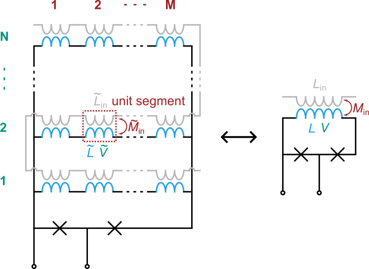
Figure 2: Schematic circuit diagram of a hypothetical $\lambda$-SQUID. The SQUID loop consists of $N$ identical segments connected in parallel, with each segment itself comprising $M$ unit elements connected in series. One such unit element is framed in red. Each unit element has an inductance $\tilde{L}$ with volume $\tilde{V}$, and couples to a unit of input loop with inductance $\tilde{L}_{\mathrm{in}}$ with a mutual inductance $\tilde{M}_{\mathrm{in}}$. The total arrangement is equivalent to a single effective $\lambda$-coil with inductance $L$, volume $V$ and mutual inductance $M_{\mathrm{in}}$ to an input coil with inductance $L_{\mathrm{in}}$.

We assume a hypothetical $\lambda$-SQUID as schematically depicted in Fig. 2. For simplicity, the flux bias coil is neglected as it does not affect the temperature sensitivity. We consider a $\lambda$-coil entirely separable into small, identical unit elements, each with inductance $\tilde{L}$ and volume $\tilde{V}$. The loop comprises $N$ parallel rows of $M$ unit elements in series each, resulting in a total of $N\times M$ unit elements in total. Each unit element couples to a segment of input coil with inductance $\tilde{L}_{\mathrm{in}}$ via a mutual inductance $\tilde{M}_{\mathrm{in}}=\kappa\sqrt{\tilde{L}\tilde{L}_{\mathrm{in}}}$. Here, $\kappa$ is the geometric coupling factor. We can thus conclude the following relations for the total loop inductance $L$ and total volume $V$ of the $\lambda$-coil and the combined mutual inductance $M_{\mathrm{in}}$ between the $\lambda$-SQUID and the input coil:

$$L = \frac{M}{N}\tilde{L}=\nu\tilde{L},$$ (1)

$$V = MN\tilde{V}=\mu\tilde{V},$$ (2)

$$M_{\mathrm{in}} = M\tilde{M}_{\mathrm{in}}=\sqrt{\nu\mu}\tilde{M}_{\mathrm{in}}.$$ (3)

With only two free parameters to choose, we see immediately that we can not choose all three quantities independently. To quantify the remaining dependence, we have introduced the two parameters $\nu=M/N$ and $\mu=MN$ that fully define a specific layout of the $\lambda$-coil.

We use the geometric parameters $\nu$ and $\mu$ to express other relevant parameters: First, we assume that our $\lambda$-SQUID is optimized in terms of noise performance [11], i.e. the SQUID screening parameter is $\beta_{\mathrm{L}}=2LI_{\mathrm{c}}/\Phi_{0}=1$ and the Stewart-McCumber parameter of the Josephson junctions is $\beta_{\mathrm{C}}=2\pi I_{\mathrm{c}}R^{2}C_{\mathrm{JJ}}/\Phi_{0}=1$. Assuming an established fabrication process for Josephson junctions, the critical current is set by the junction area $A_{\mathrm{JJ}}$ and the critical current density $j_{\mathrm{c}}$ via $I_{\mathrm{c}}=A_{\mathrm{JJ}}j_{\mathrm{c}}$. The junction capacitance consequently is $C_{\mathrm{JJ}}=A_{\mathrm{JJ}}c^{\star}_{\mathrm{JJ}}=I_{\mathrm{c}}c^{\star}_{\mathrm{JJ}}/j_{\mathrm{c}}$, with the process-specific junction capacitance per unit area $c^{\star}_{\mathrm{JJ}}$. From the conditions $\beta_{\mathrm{L}},\beta_{\mathrm{C}}=1$ we conclude:

$$I_{\mathrm{c}}=\left[\frac{\Phi_{0}}{2\tilde{L}}\right]\frac{1}{\nu},$$ (4)

$$R=\left[\sqrt{\frac{2j_{\mathrm{c}}}{\pi\Phi_{0}c^{\star}_{\mathrm{JJ}}}}\tilde{L}\right]\nu.$$ (5)

In each expression, the term in brackets is independent of the specific design of the $\lambda$-SQUID, and depends only on fabrication parameters and the design of a unit element of the $\lambda$-coil.

The noise contribution $S_{\mathrm{E,SQ}}$ caused by the $\lambda$-SQUID, expressed in fluctuations of the energy content, is given by the expression

$$S_{\mathrm{E,SQ}}=S_{\mathrm{\Phi}}\left(\frac{\partial\Phi}{\partial T}\frac{\partial T}{\partial E}\right)^{-2}.$$ (6)

Here, $S_{\mathrm{\Phi}}$ denotes the magnetic flux noise of the SQUID. Moreover, $\frac{\partial\Phi}{\partial T}$ and $\frac{\partial T}{\partial E}=1/C_{\mathrm{tot}}$ are the temperature-to-flux transfer coefficient of the $\lambda$-SQUID and the inverse total heat capacity of the detector, respectively. For an optimized dc-SQUID, the flux noise can be approximated by $S_{\mathrm{\Phi}}\approx 18k_{\mathrm{B}}TL^{2}/R$ at the operating temperature $T$ [12]. The total heat capacity of the detector comprises both, the absorber and the $\lambda$-coil, i.e. $C_{\mathrm{tot}}=C_{\mathrm{abs}}+\mu\tilde{V}c$, with $c$ the specific heat per unit volume of the $\lambda$-coil. The temperature-to-flux transfer coefficient $\frac{\partial\Phi}{\partial T}$ of the $\lambda$-SQUID is given by

$$\frac{\partial\Phi}{\partial T}=I_{\mathrm{in}}\frac{\partial M_{\mathrm{in}}}{\partial T}=\left[I_{\mathrm{in}}\frac{\partial\tilde{M}_{\mathrm{in}}}{\partial T}\right]\sqrt{\mu\nu},$$ (7)

where, again, the term in brackets does not depend on the design of the $\lambda$-coil as a whole, but rather on the unit element. Using Eq. 4 and Eq. 5 we obtain for the noise contribution

$$S_{\mathrm{E,SQ}} = 18k_{\mathrm{B}}T\sqrt{\frac{\pi\Phi_{0}c^{\star}_{\mathrm{JJ}}}{2j_{\mathrm{c}}}}\tilde{L}\nu\left(\left[I_{\mathrm{in}}\frac{\partial\tilde{M}_{\mathrm{in}}}{\partial T}\right]\sqrt{\mu\nu}\frac{1}{C_{\mathrm{abs}}+\mu\tilde{V}c}\right)^{-2}$$ (8)

$$= \left[18k_{\mathrm{B}}T\sqrt{\frac{\pi\Phi_{0}c^{\star}_{\mathrm{JJ}}}{2j_{\mathrm{c}}}}\frac{\tilde{L}}{I_{\mathrm{in}}^{2}\left(\frac{\partial\tilde{M}_{\mathrm{in}}}{\partial T}\right)^{2}}\right]\frac{\left(C_{\mathrm{abs}}+\mu\tilde{V}c\right)^{2}}{\mu}=\eta g\left(\mu\right).$$ (9)

Here, we have introduced the substitutions

$$\eta = \left[18k_{\mathrm{B}}T\sqrt{\frac{\pi\Phi_{0}c^{\star}_{\mathrm{JJ}}}{2j_{\mathrm{c}}}}\frac{\tilde{L}}{I_{\mathrm{in}}^{2}\left(\frac{\partial\tilde{M}_{\mathrm{in}}}{\partial T}\right)^{2}}\right]\quad\mathrm{and}$$ (10)

$$g\left(\mu\right) = \frac{\left(C_{\mathrm{abs}}+\mu\tilde{V}c\right)^{2}}{\mu}.$$ (11)

We see that $S_{\mathrm{E,SQ}}$ neatly separates into a term $\eta$ which depends only on the unit element, but is independent of the specific layout of the $\lambda$-coil, and a function $g\left(\mu\right)$, which contains the dependence of the $\lambda$-SQUID noise $S_{\mathrm{E,SQ}}$ on the arrangement of unit elements that comprises the $\lambda$-coil. It is interesting to note that only $\mu$ appears here, and that the parameter $\nu$ has dropped out. This can be understood as follows: An increase in $\nu$ causes a proportional increase in total inductance $L$ and a rise of $M_{\mathrm{in}}\propto\sqrt{\nu}$. While the latter results in an increase of detector signal, the former affects the flux noise negatively. Ultimately, the signal-to-noise of the $\lambda$-SQUID remains unaltered by a change of the inductance $L$ by varying the parameter $\nu$ as introduced above.

To minimize the noise level $S_{\mathrm{E,SQ}}$, we only have to consider the design parameter $\mu$. Since the prefactor $\eta$ has no influence on this optimization, we restrict our efforts to the function $g\left(\mu\right)$ and find

$$\frac{\partial g\left(\mu\right)}{\partial\mu} = \frac{2\left(C_{\mathrm{abs}}+\mu\tilde{V}c\right)c\tilde{V}}{\mu}-\frac{\left(C_{\mathrm{abs}}+\mu\tilde{V}c\right)^{2}}{\mu^{2}}$$ (12)

$$\frac{\partial^{2}g\left(\mu\right)}{\partial\mu^{2}} = \frac{2\left(c\tilde{V}\right)^{2}}{\mu}-\frac{4\left(C_{\mathrm{abs}}+\mu\tilde{V}c\right)c\tilde{V}}{\mu^{2}}+\frac{2\left(C_{\mathrm{abs}}+\mu\tilde{V}c\right)^{2}}{\mu^{3}}$$ (13)

for its first and second derivative. In this way, we find that the function $g\left(\mu\right)$, and thus the $\lambda$-SQUID energy noise contribution $S_{\mathrm{E,SQ}}$, has a minimum if the condition $\mu=\mu_{\mathrm{opt}}$ is satisfied, with

$$\mu_{\mathrm{opt}}c\tilde{V}=C_{\mathrm{sens}}=C_{\mathrm{abs}}.$$ (14)

Thus, we can conclude that the layout of the $\lambda$-coil should be chosen such that the total specific heat of the $\lambda$-coil exactly equals the specific heat of the absorber $C_{\mathrm{sens}}=C_{\mathrm{abs}}$. This resembles a well-known result for cryogenic microcalorimeters [13].

3 Conclusion

The recently proposed $\lambda$-SQUID is a superconducting microcalorimeter with in-situ tunable gain and, with a proper choice of absorber and sensor material, promises to reach sub-eV energy resolution. In preparation for such a demonstration, we have presented theoretical design considerations related to the optimization of the layout of the $\lambda$-coil, which is the fundamental sensing element of a $\lambda$-SQUID. By sub-dividing the $\lambda$-coil into a large number of small unit elements, we could abstract the layout of any possible design of the $\lambda$-coil for a given fabrication method, and describe the remaining degrees of freedom in the design process by two parameters $\mu$ and $\nu$. When considering the influence of these parameters on the energy noise contribution $S_{\mathrm{E,SQ}}$ of the $\lambda$-SQUID, we draw two conclusions. First, the total inductance $L$ of the $\lambda$-coil has no effect on the resulting energy noise, and can thus be chosen freely. Second, the noise contribution $S_{\mathrm{E,SQ}}$ is minimized if the total volume of the $\lambda$-coil is chosen such that its specific heat directly equals that of the X-ray absorber: $C_{\mathrm{sens}}=C_{\mathrm{abs}}$.

Acknowledgments C. Schuster acknowledges financial support by the Karlsruhe School of Elementary Particle and Astroparticle Physics: Science and Technology (KSETA).

References

- \bibcommenthead
- Irwin and Hilton [2005] Irwin, K.D., Hilton, G.C.: In: Enss, C. (ed.) Transition-Edge Sensors, pp. 63–150. Springer, Berlin, Heidelberg (2005). https://doi.org/10.1007/10933596_3 . {https://doi.org/10.1007/10933596_3}
- Ullom and Bennett [2015] Ullom, J.N., Bennett, D.A.: Review of superconducting transition-edge sensors for x-ray and gamma-ray spectroscopy. Superconductor Science and Technology 28(8), 084003 (2015) https://doi.org/10.1088/0953-2048/28/8/084003
- Fleischmann et al. [2005] Fleischmann, A., Enss, C., Seidel, G.M.: In: Enss, C. (ed.) Metallic Magnetic Calorimeters, pp. 151–216. Springer, Berlin, Heidelberg (2005). https://doi.org/10.1007/10933596_4 . https://doi.org/10.1007/10933596_4
- Kempf et al. [2018] Kempf, S., Fleischmann, A., Gastaldo, L., Enss, C.: Physics and Applications of Metallic Magnetic Calorimeters. Journal of Low Temperature Physics, 1–15 (2018) https://doi.org/10.1007/s10909-018-1891-6
- Uhlig et al. [2015] Uhlig, J., Doriese, W.B., Fowler, J.W., Swetz, D.S., Jaye, C., Fischer, D.A., Reintsema, C.D., Bennett, D.A., Vale, L.R., Mandal, U., O’Neil, G.C., Miaja-Avila, L., Joe, Y.I., El Nahhas, A., Fullagar, W., Parnefjord Gustafsson, F., Sundström, V., Kurunthu, D., Hilton, G.C., Schmidt, D.R., Ullom, J.N.: High-resolution X-ray emission spectroscopy with transition-edge sensors: present performance and future potential. Journal of Synchrotron Radiation 22(3), 766–775 (2015) https://doi.org/10.1107/S1600577515004312
- Friedrich [2006] Friedrich, S.: Cryogenic x-ray detectors for synchrotron science. J Synchrotron Radiat 13(Pt 2), 159–71 (2006) https://doi.org/%****␣_main.bbl␣Line␣150␣****10.1107/S090904950504197X
- Doriese et al. [2016] Doriese, W.B., Morgan, K.M., Bennett, D.A., Denison, E.V., Fitzgerald, C.P., Fowler, J.W., Gard, J.D., Hays-Wehle, J.P., Hilton, G.C., Irwin, K.D., Joe, Y.I., Mates, J.A.B., O’Neil, G.C., Reintsema, C.D., Robbins, N.O., Schmidt, D.R., Swetz, D.S., Tatsuno, H., Vale, L.R., Ullom, J.N.: Developments in Time-Division Multiplexing of X-ray Transition-Edge Sensors. Journal of Low Temperature Physics 184, 389–395 (2016) https://doi.org/10.1007/s10909-015-1373-z
- Lee et al. [2015] Lee, S.J., Adams, J.S., Bandler, S.R., Chervenak, J.A., Eckart, M.E., Finkbeiner, F.M., Kelley, R.L., Kilbourne, C.A., Porter, F.S., Sadleir, J.E., Smith, S.J., Wassell, E.J.: Fine pitch transition-edge sensor X-ray microcalorimeters with sub-eV energy resolution at 1.5 keV. Applied Physics Letters 107(22), 223503 (2015) https://doi.org/10.1063/1.4936793 https://pubs.aip.org/aip/apl/article-pdf/doi/10.1063/1.4936793/14472862/223503_1_online.pdf
- Krantz et al. [2023] Krantz, M., Toschi, F., Maier, B., Heine, G., Enss, C., Kempf, S.: Magnetic microcalorimeter with paramagnetic temperature sensors and integrated dc-squid readout for high-resolution x-ray emission spectroscopy. arXiv (2023) arXiv:2310.08698 [physics.ins-det]
- Schuster and Kempf [2023] Schuster, C., Kempf, S.: Squid-based superconducting microcalorimeter with in-situ tunable gain. arXiv (2023) arXiv:2310.03489 [physics.ins-det]
- Tesche and Clarke [1977] Tesche, C.D., Clarke, J.: dc SQUID: Noise and optimization. Journal of Low Temperature Physics 29, 301–331 (1977) https://doi.org/10.1007/BF00655097
- Chesca et al. [2004] Chesca, B., Kleiner, R., Koelle, D.: In: The SQUID Handbook, pp. 29–92. John Wiley & Sons, Ltd (2004). Chap. SQUID Theory. https://doi.org/10.1002/3527603646.ch2 . https://onlinelibrary.wiley.com/doi/abs/10.1002/3527603646.ch2
- McCammon [2005] McCammon, D.: In: Enss, C. (ed.) Thermal Equilibrium Calorimeters – An Introduction, pp. 1–34. Springer, Berlin, Heidelberg (2005). https://doi.org/10.1007/10933596_1 . https://doi.org/10.1007/10933596_1