Towards Self-Interpretable
Graph-Level Anomaly Detection

Abstract

Graph-level anomaly detection (GLAD) aims to identify graphs that exhibit notable dissimilarity compared to the majority in a collection. However, current works primarily focus on evaluating graph-level abnormality while failing to provide meaningful explanations for the predictions, which largely limits their reliability and application scope. In this paper, we investigate a new challenging problem, explainable GLAD, where the learning objective is to predict the abnormality of each graph sample with corresponding explanations, i.e., the vital subgraph that leads to the predictions. To address this challenging problem, we propose a Self-Interpretable Graph aNomaly dETection model (SIGNET for short) that detects anomalous graphs as well as generates informative explanations simultaneously. Specifically, we first introduce the multi-view subgraph information bottleneck (MSIB) framework, serving as the design basis of our self-interpretable GLAD approach. This way SIGNET is able to not only measure the abnormality of each graph based on cross-view mutual information but also provide informative graph rationales by extracting bottleneck subgraphs from the input graph and its dual hypergraph in a self-supervised way. Extensive experiments on 16 datasets demonstrate the anomaly detection capability and self-interpretability of SIGNET.

1 Introduction

Graphs are ubiquitous data structures in numerous domains, including chemistry, traffic, and social networks [1, 2, 3]. Among machine learning tasks for graph data, graph-level anomaly detection (GLAD) is a challenge that aims to identify the graphs that exhibit substantial dissimilarity from the majority of graphs in a collection [4]. GLAD presents great potential for various real-world scenarios, such as toxic molecule recognition [5] and pathogenic brain mechanism discovery [6]. Recently, GLAD has drawn increasing research attention, with advanced techniques being applied to this task, e.g., knowledge distillation [4] and one-class classification [7].

Despite their promising performance, existing works [4, 7, 8, 9] mainly aim to answer how to predict abnormal graphs by designing various GLAD architectures; however, they fail to provide explanations for the prediction, i.e., illustrating why these graphs are recognized as anomalies. In real-world applications, it is of great significance to make anomaly detection models explainable [10]. From the perspective of models, valid explainability makes GLAD models trustworthy to meet safety and security requirements [11]. For example, an explainable fraud detection model can pinpoint specific fraudulent behaviors when identifying defrauders, which enhances the reliability of predictions. From the perspective of data, an anomaly detection model with explainability can help us explicitly understand the anomalous patterns of the dataset, which further supports human experts in data understanding [12]. For instance, an explainable GLAD model for molecules can summarize the functional groups that cause abnormality, enabling researchers to deeply investigate the properties of compounds. Hence, the broad applications of interpreting anomaly detection results motivate us to investigate the problem of Explainable GLAD where the GLAD model is expected to measure the abnormality of each graph sample as well as provide meaningful explanations of the predictions during the inference time. As an example shown in Fig. 1, the GLAD model also extracts a graph rationale [13, 14] corresponding to the predicted anomaly score. Although there are a few studies [10, 15, 16] proposed to explain anomaly detection results for visual or tabular data, explainable GLAD remains underexplored and it is non-trivial to apply those methods to our problem due to the discrete nature of irregular graph-structured data [17].

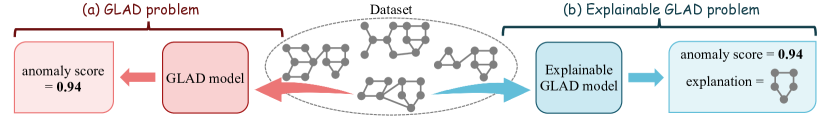
Figure 1: A toy example to illustrate (a) GLAD problem and (b) explainable GLAD problem.

Towards the goal of designing an explainable GLAD model, two essential challenges need to be solved with careful design: Challenge 1 — how to make the GLAD model self-interpretable? Even though we can leverage existing post-hoc explainers [19, 20] for GNNs to explain the predictions of the GLAD model, such post-hoc explainers are not synergistically learned with the detection models, resulting in the risk of wrong, biased, and sub-optimal explanations [21, 22]. Hence, developing a self-interpretable GLAD model which detects graph-level anomalies with explanations inherently is more desirable and requires urgent research efforts. Challenge 2 — how to learn meaningful graph explanations without using supervision signals? For the problem of GLAD, ground-truth anomalies are usually unavailable during training, raising significant challenges to both detecting anomalies and providing meaningful explanations. Since most of the existing self-interpretable GNNs [13, 21, 22] merely focus on the (semi-)supervised setting, in particular the node/graph classification tasks, how to design a self-interpretable model for the explainable GLAD problem where ground-truth labels are inaccessible remains a challenging task.

To solve the above challenges, in this paper, we develop a novel Self-Interpretable Graph aNomaly dETection model (SIGNET for short). Based on the information bottleneck (IB) principle, we first propose a multi-view subgraph information bottleneck (MSIB) framework, serving as the design basis of our self-interpretable GLAD model. Under the MSIB framework, the instantiated GLAD model is able to predict the abnormality of each graph as well as generate corresponding explanations without relying on ground-truth anomalies simultaneously. To learn the self-interpretable GLAD model without ground-truth anomalies, we introduce the dual hypergraph as a supplemental view of the original graph and employ a unified bottleneck subgraph extractor to extract corresponding graph rationales. By further conducting multi-view learning among the extracted graph rationales, SIGNET is able to learn the feature patterns from both node and edge perspectives in a purely self-supervised manner. During the test phase, we can directly measure the abnormality of each graph sample based on its inter-view agreement (i.e., cross-view mutual information) and derive the corresponding graph rationales for the purpose of explaining the prediction. To sum up, our contribution is three-fold:

• Problem. We propose to investigate the explainable GLAD problem that has broad application prospects. To the best of our knowledge, this is the first attempt to study the explainability problem for graph-level anomaly detection.

• Algorithm. We propose a novel self-interpretable GLAD model termed SIGNET, which infers graph-level anomaly scores and subgraph-level explanations simultaneously with the multi-view subgraph information bottleneck framework.

• Evaluation. We perform extensive experiments to corroborate the anomaly detection performance and self-interpretation ability of SIGNET via thorough comparisons with state-of-the-art methods on 16 benchmark datasets.

2 Preliminaries and Related Work

In this section, we introduce the preliminaries and briefly review the related works. A more comprehensive literature review can be found in Appendix B.

Notations. Let $G=(\mathcal{V},\mathcal{E},\mathbf{X})$ be a simple graph with $n$ nodes and $m$ edges, where $\mathcal{V}$ is the set of nodes and $\mathcal{E}$ is the set of edges. The node features are included by feature matrix $\mathbf{X}\in\mathbb{R}^{n\times d_{f}}$, and the connectivity among the nodes is represented by adjacency matrix $\mathbf{A}\in\mathbb{R}^{n\times n}$. Unlike simple graphs where each edge only connects two nodes, “hypergraph” is a generalization of a traditional graph structure in which hyperedges connect more than two nodes. We define a hypergraph with $n^{*}$ nodes and $m^{*}$ hyperedges as $G^{*}=(\mathcal{V}^{*},\mathcal{E}^{*},\mathbf{X}^{*})$, where $\mathcal{V}^{*}$, $\mathcal{E}^{*}$, and $\mathbf{X}^{*}\in\mathbb{R}^{n^{*}\times d_{f}^{*}}$ are the node set, hyperedge set, and node feature matrix respectively. To indicate the higher-order relations among arbitrary numbers of nodes within a hypergraph, we use an incidence matrix $\mathbf{M}^{*}\in\mathbb{R}^{n^{*}\times m^{*}}$ to represent the interaction between $n^{*}$ nodes and $m^{*}$ hyperedges. Alternatively, a simple graph and a hypergraph and be represented by $G=(\mathbf{A},\mathbf{X})$ and $G^{*}=(\mathbf{M}^{*},\mathbf{X}^{*})$, respectively. We denote the Shannon mutual information (MI) of two random variables $A$ and $B$ as $I(A;B)$.

Graph Neural Networks (GNNs). GNNs are the extension of deep neural networks onto graph data, which have been applied to various graph learning tasks [1, 2, 23, 24, 25, 26, 27, 28]. Mainstream GNNs usually follow the paradigm of message passing [2, 23, 24, 26]. Some studies termed hypergraph neural networks (HGNNs) also apply GNNs to hypergraphs [29, 30, 31]. The formulations of GNN and HGNN are in Appendix C. To make the predictions understandable, some efforts try to uncover the explanation for GNNs [18, 32]. A branch of methods, termed post-hoc GNN explainers, use specialized models to explain the behavior of a trained GNN [19, 20, 33]. Meanwhile, some self-interpretable GNNs can intrinsically provide explanations for predictions using interpretable designs in GNN architectures [13, 21, 22]. While these methods mainly aim at supervised classification scenarios, how to interpret unsupervised anomaly detection models still remains open.

Information Bottleneck (IB). IB is an information theory-based approach for representation learning that trains the encoder by preserving the information that is relevant to label prediction while minimizing the amount of superfluous information [34, 35, 36]. Formally, given the data $X$ and the label $Y$, IB principle aims to find the representation $Z$ by maximizing the following objective: $\max_{Z}I(Z;Y)-\beta I(X;Z)$, where $\beta$ is a hyper-parameter to trade off informativeness and compression. To extend IB onto unsupervised learning scenarios, Multi-view Information Bottleneck (MIB) [37] provides an optimizable target for unsupervised multi-view learning, which alleviates the reliance on label $Y$. Given two different and distinguishable views $V_{1}$ and $V_{2}$ of the same data $X$, the objective of MIB is to learn sufficient and compact representations $Z_{1}$ and $Z_{2}$ for two views respectively. Taking view $V_{1}$ as an example, by factorizing the MI between $V_{1}$ and $Z_{1}$, we can identify two components: $I(V_{1};Z_{1})=I(V_{1};Z_{1}|V_{2})+I(V_{2};Z_{1})$, where the first term is the superfluous information that is expected to be minimized, and the second term is the predictive information that should be maximized. Then, $Z_{1}$ can be learned using a relaxed Lagrangian objective:

$$\max_{Z_{1}}I(V_{2};Z_{1})-\beta_{1}I(V_{1};Z_{1}|V_{2}),$$ (1)

where $\beta_{1}$ is a trade-off parameter. By optimizing Eq. (1) and its counterpart in view $V_{2}$, we can learn informative and compact $Z_{1}$ and $Z_{2}$ by extracting the information from each other.

IB principle is also proven to be effective in graph learning tasks, such as graph contrastive learning [38, 39], subgraph recognition [17, 40], graph-based recommendation [41], and robust graph representation learning [22, 42, 43]. Nevertheless, how to leverage the idea of IB on graph anomaly detection tasks is still an open problem.

Graph-level Anomaly Detection (GLAD). GLAD aims to recognize anomalous graphs from a set of graphs by learning an anomaly score for each graph sample to indicate its degree of abnormality [4, 7, 8, 9]. Recent studies try to address the GLAD problem with various advanced techniques, such as knowledge distillation [4], one-class classification [7], transformation learning [8], and deep graph kernel [44]. However, these methods can only learn the anomaly score but fail to provide explanations, i.e., the graph rationale causing the abnormality, for their predictions.

Problem Formulation. Based on this mainstream unsupervised GLAD paradigm [4, 7, 8], in this paper, we present a novel research problem termed explainable GLAD, where the GLAD model is expected to provide the anomaly score as well as the explanations of such a prediction for each testing graph sample. Formally, the proposed research problem can be formulated by:

Definition 2.1 (Explainable graph-level anomaly detection).

Given the training set $\mathcal{G}_{tr}$ that contains a number of normal graphs, we aim at learning an explainable GLAD model $f:\mathbb{G}\to(\mathbb{R},\mathbb{G})$ that is able to predict the abnormality of a graph and provide corresponding explanations. In specific, given a graph $G_{i}$ from the test set $\mathcal{G}_{te}$ with normal and abnormal graphs, the model can generate an output pair $f(G_{i})=(s_{i},G^{(es)}_{i})$, where $s_{i}$ is the anomaly score that indicates the abnormality degree of $G_{i}$, and $G^{(es)}_{i}$ is the subgraph of $G_{i}$ that explains why $G_{i}$ is identified as a normal/abnormal sample.

3 Methodology

This section details the proposed model SIGNET for explainable GLAD. Firstly, we derive a multi-view subgraph information bottleneck (MSIB) framework (Sec. 3.1) that allows us to identify anomalies with causal interpretations provided. Then, we provide the instantiation of the components in MSIB framework, including view construction (Sec. 3.2), bottle subgraph extraction (Sec. 3.3), and cross-view mutual information (MI) maximization (Sec. 3.4), which compose the SIGNET model. Finally, we introduce the self-interpretable GLAD inference (Sec. 3.5) of SIGNET. The overall learning pipeline of SIGNET is demonstrated in Fig. 2(a).

3.1 MSIB Framework Overview

To achieve the goal of self-interpretable GLAD, an unsupervised learning approach that can jointly predict the abnormality of graphs and yield corresponding explanations is required. Inspired by the concept of information bottleneck (IB) and graph multi-view learning [36, 37, 45], we propose multi-view subgraph information bottleneck (MSIB), a self-interpretable and self-supervised learning framework for GLAD. The learning objective of MSIB is to optimize the “bottleneck subgraphs”, the vital substructure on two distinct views of a graph, by maximizing the predictive structural information shared by both graph views while minimizing the superfluous information that is irrelevant to the cross-view agreement. Such an objective can be optimized in a self-supervised manner, without the guidance of ground-truth labels. Due to the observation that latent anomaly patterns of graphs can be effectively captured by multi-view learning [8, 9], we can directly use the cross-view agreement, i.e., the MI between two views, to evaluate the abnormality of a graph sample. Simultaneously, the extracted bottleneck subgraphs provide us with graph rationales to explain the anomaly detection predictions, since they contain the most compact substructure sourced from the original data and the most discriminative knowledge for the predicted abnormality, i.e., the estimated cross-view MI.

Formally, in the proposed MSIB framework, we assume each graph sample $G$ has two different and distinguishable views $G^{1}$ and $G^{2}$. Then, taking view $G^{1}$ as an example, the target of MSIB is to learn a bottleneck subgraph $G^{1(s)}$ for $G^{1}$ by optimizing the following objective:

$$\max_{G^{1(s)}}I(G^{2};G^{1(s)})-\beta_{1}I(G^{1};G^{1(s)}|G^{2}).$$ (2)

Similar to MIB (Eq. (1), the optimization for $G^{2(s)}$, the bottleneck subgraph of $G^{2}$, can be written in the same format. Then, by parameterizing bottleneck subgraph extraction and unifying the domain of bottleneck subgraphs, the objective can be transferred to minimize a tractable loss function:

$$\mathcal{L}_{MSIB}=-I(G^{1(s)};G^{2(s)})+\beta D_{SKL}\left(p_{\theta}(G^{1(s)}|G^{1})\|p_{\psi}(G^{2(s)}|G^{2})\right),$$ (3)

where $p_{\theta}(G^{1(s)}|G^{1})$ and $p_{\psi}(G^{2(s)}|G^{2})$ are the bottleneck subgraph extractors (parameterized by $\theta$ and $\psi$) for $G^{1}$ and $G^{2}$ respectively, $D_{SKL}(\cdot)$ is the symmetrized Kullback–Leibler (SKL) divergence, and $\beta$ is a trade-off hyper-parameter. Detailed deductions from Eq. (2) to Eq. (3) are in Appendix D.

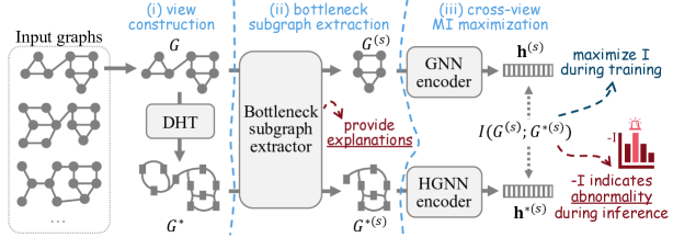
(a) The overall pipeline of SIGNET

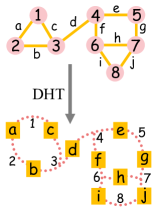
(b) DHT

Figure 2: (a) The overall pipeline of the proposed model SIGNET, consisting of (i) view construction, (ii) bottleneck subgraph extraction, and (iii) cross-view MI maximization. (b) An illustration of dual hypergraph transformation (DHT), where the nodes (●) and edges (—) in the original graph correspond to hyperedges ($\mathbf{\cdots}$) and nodes ($\blacksquare$) in its dual hypergraph, respectively.

MSIB framework can guide us to build a self-interpretable GLAD model. The first term in Eq. (3) tries to maximize the MI between the bottleneck subgraphs from two views, which not only prompts the model to capture vital subgraphs but also helps capture the cross-view matching patterns for anomaly detection. The second term in Eq. (3) is a regularization term to align the extractors, which ensures the compactness of bottleneck subgraphs. During inference, $-I(G^{1(s)};G^{2(s)})$ can be regarded as a measure of abnormality. Meanwhile, the bottleneck subgraphs extracted by $p_{\theta}$ and $p_{\psi}$ can serve as explanations. In the following subsections, we take SIGNET as a practical implementation of MSIB framework. We illustrate the instantiations of view construction ($G^{1}$ and $G^{2}$), subgraph extractors ($p_{\theta}$ and $p_{\psi}$), MI estimation ($I(G^{1(s)};G^{2(s)})$), and explainable GLAD inference, respectively.

3.2 Dual Hypergraph-based View Construction

To implement MSIB framework for GLAD, the first step is to construct two different and distinguishable views $G^{1}$ and $G^{2}$ for each sample $G$. In multi-view learning approaches [37, 46, 47, 48], a general strategy is using stochastic perturbation-based data augmentation (e.g., edge modification [46] and feature perturbation [47]) to create multiple views. Despite their success in graph representation learning [46, 47, 48], we claim that perturbation-based view constructions are not appropriate in SIGNET for the following reasons. 1) Low sensitivity to anomalies. Due to the similarity of normal and anomalous graphs in real-world data, perturbations may create anomaly-like data from normal data as the augmented view [49]. In this case, maximizing the cross-view MI would result in reduced sensitivity of the model towards distinguishing between normal and abnormal data, hindering the performance of anomaly detection [50]. 2) Less differentiation. In the principle of MIB, two views should be distinguishable and mutually redundant [37]. However, the views created by graph perturbation from the same sample can be similar to each other, which violates the assumption of our basic framework. 3) Harmful instability. The MI $I(G^{1(s)};G^{2(s)})$ for abnormality measurement is highly related to the contents of two views. Nevertheless, the view contents generated by stochastic perturbation can be quite unstable due to the randomness, leading to inaccurate estimation of abnormality.

Considering the above limitations, a perturbation-free, distinct, and stable strategy is required for view construction. To this end, we utilize dual hypergraph transformation (DHT) [51] to construct the opposite view of the original graph. Concretely, for a graph sample $G$, we define the first view as itself (i.e., $G^{1}=G$) and the second view as its dual hypergraph $G^{*}$ (i.e., $G^{2}=G^{*}$). Based on the hypergraph duality [52, 53], dual hypergraph can be acquired from the original simple graph with DHT: each edge of the original graph is transformed into a node of the dual hypergraph, and each node of the original graph is transformed into a hyperedge of the dual hypergraph [51]. As the example shown in Fig. 2(b), the structural roles of nodes and edges are interchanged by DHT, and the incidence matrix $\mathbf{M}^{*}$ of the dual hypergraph is the transpose of the incidence matrix of the original graph. To initialize the node features $\mathbf{X}^{*}\in\mathbb{R}^{m\times d_{f}^{*}}$ of $G^{*}$, we can either use the original edge features (if available), or construct edge-level features from the original node features or according to edge-level geometric property.

The DHT-based view construction brings several advantages. Firstly, the dual hypergraph has significantly distinct contents from the original view, which caters to the needs for differentiation in MIB. Secondly, the dual hypergraph pays more attention to the edge-level information, encouraging the model to capture not only node-level but also edge-level anomaly patterns. Thirdly, DHT is a bijective mapping between two views, avoiding confusion between normal and abnormal samples. Fourthly, DHT is randomness-free, ensuring the stable estimation of MI.

3.3 Bottleneck Subgraph Extraction

In MSIB framework, bottleneck subgraph extraction is a key component that learns to refine the core rationale for abnormality explanations. Following the procedure of MSIB, we need to establish two bottleneck subgraph extractors for the original view $G$ and dual hypergraph view $G^{*}$ respectively. To model the discrete subgraph extraction process in a differentiable manner with neural networks, following previous methods [14, 17, 22], we introduce continuous relaxation into the subgraph extractors. Specifically, for the original view $G$, we model the subgraph extractor with $p_{\theta}(G^{(s)}|G)=\prod_{v\in\mathcal{V}}p_{\theta}(v\in\mathcal{V}^{(s)}|G)$. In practice, the GNN-based extractor takes $G$ as input and outputs a node probability vector $\mathbf{p}\in\mathbb{R}^{n\times 1}$, where each entry indicates the probability that the corresponding node belongs to $G^{(s)}$. Similarly, for the dual hypergraph view $G^{*}$, an edge-centric HGNN serves as the subgraph extractor $p_{\psi}$. It takes $G^{*}$ as input and outputs an edge probability vector $\mathbf{p}^{*}\in\mathbb{R}^{m\times 1}$ that indicates if the dual nodes (corresponding to the edges in the original graphs) belong to $G^{*(s)}$. Once the probability vectors are calculated, the subgraph extraction can be executed by:

$$G^{(s)}=(\mathbf{A},\mathbf{X}^{(s)})=(\mathbf{A},\mathbf{X}\odot\mathbf{p}),\quad G^{*(s)}=(\mathbf{M}^{*},\mathbf{X}^{*(s)})=(\mathbf{M}^{*},\mathbf{X}^{*}\odot\mathbf{p}^{*}),$$ (4)

where $\odot$ is the row-wise production. Then, to implement the second term in Eq. (3), we can lift the node probabilities $\mathbf{p}$ to edge probabilities by $\mathbf{p}^{\prime}$ by $\mathbf{p}^{\prime}_{\mathbb{I}(e_{ij})}=\mathbf{p}_{i}\mathbf{p}_{j}$, where $\mathbb{I}(e_{ij})$ is the index of edge connecting node $v_{i}$ and $v_{j}$. After re-probabilizing $\mathbf{p}^{\prime}$, the SKL divergence between $\mathbf{p}^{\prime}$ and $\mathbf{p}^{*}$ can be computed as the regularization term in MSIB framework.

Although the above “two-extractor” design correlates to the theoretical framework of MSIB, in practice, it is non-trivial to ensure the consistency of two generated subgraphs only with an SKL divergence loss. The main reason is that the input and architectures of two extractors are quite different, leading to the difficulty in output alignment. However, the consistency of two bottleneck subgraphs not only guarantees the informativeness of cross-view MI for abnormality measurement, but also affects the quality of explanations. Considering the significance of preserving consistency, we use a single extractor to generate bottleneck subgraphs for two views. In specific, the bottleneck subgraph extractor first takes the original graph $G$ as its input and outputs the node probability vector $\mathbf{p}$ for the bottleneck subgraph extraction of $G^{(s)}$. Then, leveraging the node-edge correspondence in DHT, we can directly lift the node probabilities to edge probability vector $\mathbf{p}^{*}$ via $\mathbf{p}^{*}_{\mathbb{I}(e_{ij})}=\mathbf{p}_{i}\mathbf{p}_{j}$ and re-probabilization operation. $\mathbf{p}^{*}$ can be used to extract subgraph for the dual hypergraph view. In this way, the generated bottleneck subgraphs in two views can be highly correlated, enhancing the quality of GLAD prediction (MI) and its explanations. Meanwhile, such a “single-extractor” design further simplifies the model architecture by removing extra extractor and loss function (i.e., the $D_{SKL}$ term in Eq. (3)), reducing the model complexity. Empirical comparison in Sec. 4.4 also validates the effectiveness of this design.

3.4 Cross-view MI Maximization

After bottleneck subgraph extraction, the next step is to maximize the MI $I(G^{(s)};G^{*(s)})$ between the bottleneck subgraphs from two views. The estimated MI, in the testing phase, can be used to evaluate the graph-level abnormality. Owing to the discrete and complex nature of graph-structured data, it is difficult to directly estimate the MI between two subgraphs. Alternatively, a feasible solution is to obtain compact representations for two subgraphs, and then, calculate the representation-level MI as a substitute. In SIGNET, we use message passing-based GNN and HGNN with pooling layer (formulated in Appendix C) to learn the subgraph representations $\mathbf{h}_{G^{(s)}}$ and $\mathbf{h}_{G^{*(s)}}$ for $G^{(s)}$ and $G^{*(s)}$, respectively. In this case, $I(G^{(s)};G^{*(s)})$ can be transferred into a tractable term, i.e., the MI between subgraph representations $I(\mathbf{h}_{G^{(s)}};\mathbf{h}_{G^{*(s)}})$.

After that, the MI term $I(\mathbf{h}_{G^{(s)}};\mathbf{h}_{G^{*(s)}})$ can be maximized by using sample-based differentiable MI lower bounds [37], such as Jensen-Shannon (JS) estimator [54], Donsker-Varadhan (DV) estimator [55], and Info-NCE estimator [56]. Due to its strong robustness and generalization ability [37, 57], we employ Info-NCE for MI estimation in SIGNET. Specifically, given a batch of graph samples $\mathcal{B}=\{G_{1},\cdots,G_{B}\}$, the training loss of SIGNET can be written by:

$$\mathcal{L}=-\frac{1}{2|\mathcal{B}|}\sum_{G_{i}\in\mathcal{B}}I(\mathbf{h}_{G^{(s)}_{i}};\mathbf{h}_{G^{*(s)}_{i}}) =-\frac{1}{2|\mathcal{B}|}\sum_{G_{i}\in\mathcal{B}}\left(\ell(\mathbf{h}_{G^{(s)}_{i}},\mathbf{h}_{G^{*(s)}_{i}})+\ell(\mathbf{h}_{G^{*(s)}_{i}},\mathbf{h}_{G^{(s)}_{i}})\right),$$ (5)

$$\ell(\mathbf{h}_{G^{(s)}_{i}},\mathbf{h}_{G^{*(s)}_{i}}) =\operatorname{log}\frac{exp{\left({f_{k}}(\mathbf{h}_{G^{(s)}_{i}},\mathbf{h}_{G^{*(s)}_{i}})/\tau\right)}}{\sum_{G_{j}\in\mathcal{B}\backslash G_{i}}exp{\left({f_{k}}(\mathbf{h}_{G^{(s)}_{i}},\mathbf{h}_{G^{(s)}_{j}})/\tau\right)}},$$

where $f_{k}(\cdot,\cdot)$ is the cosine similarity function, $\tau$ is the temperature hyper-parameter, and $\ell(\mathbf{h}_{G^{*(s)}_{i}},\mathbf{h}_{G^{(s)}_{i}})$ is calculated following $\ell(\mathbf{h}_{G^{(s)}_{i}},\mathbf{h}_{G^{*(s)}_{i}})$.

3.5 Self-Interpretable GLAD Inference

In this subsection, we introduce the self-interpretable GLAD inference protocol with SIGNET (marked in red in Fig. 2(a)) that is composed of two parts: anomaly scoring and explanation.

Anomaly scoring. By minimizing Eq. (5) on training data, the cross-view matching patterns of normal samples are well captured, leading to a higher MI for normal data; on the contrary, the anomalies with anomalous attributal and structural characteristics tend to violate the matching patterns, resulting in their lower cross-view MI in our model. Leveraging this property, during inference, the negative of MI can indicate the abnormality of testing data. For a testing sample $G_{i}$, its anomaly score $s_{i}$ can be calculated by $s_{i}=-I(\mathbf{h}_{G^{(s)}_{i}};\mathbf{h}_{G^{*(s)}_{i}})$, where the MI is estimated by Info-NCE.

Explanation. In SIGNET, the bottleneck subgraph extractor is able to pinpoint the key substructure of the input graph under the guidance of MSIB framework. The learned bottleneck subgraphs are the most discriminative components of graph samples and are highly related to the anomaly scores. Therefore, we can directly regard the bottleneck subgraphs as the explanations of anomaly detection results. In specific, the node probabilities $\mathbf{p}$ and edge probabilities $\mathbf{p}^{*}$ can indicate the significance of nodes and edges, respectively. In practical inference, we can pick the nodes/edges with top-k probabilities or use a threshold-based strategy to acquire a fixed-size explanation subgraph $G^{(es)}$.

More discussion about methodology, including the pseudo-code algorithm of SIGNET, the comparison between SIGNET and existing method, and the complexity analysis of SIGNET, is illustrated in Appendix E.

4 Experiments

In this section, extensive experiments are conducted to answer three research questions:

• RQ1: Can SIGNET provide informative explanations for the detection results?

• RQ2: How effective is SIGNET on identifying anomalous graph samples?

• RQ3: What are the contributions of the core designs in SIGNET model?

4.1 Experimental Setup

Datasets. For the explainable GLAD task, we introduce 6 datasets with ground-truth explanations, including three synthetic datasets and three real-world datasets. Details are demonstrated below. We also verify the anomaly detection performance of SIGNET on 10 TU datasets [58], following the setting in [4]. Detailed statistics and visualization of datasets are demonstrated in Appendix F.1

• BM-MT, BM-MN, and BM-MS are three synthetic dataset created by following [13, 19]. Each graph is composed of one base (Tree, Ladder, or Wheel) and one or more motifs that decide the abnormality of the graph. For BM-MT (motif type), each normal graph has a house motif and each anomaly has a 5-cycle motif. For BM-MN (motif number), each normal graph has 1 or 2 house motifs and each anomaly has 3 or 4 house motifs. For BM-MS (motif size), each normal graph has a cycle motif with 3~5 nodes and each anomaly has a cycle motif with 6~9 nodes. The ground-truth explanations are defined as the nodes/edges within motifs.

• MNIST-0 and MNIST-1 are two GLAD datasets derived from MNIST-75sp superpixel dataset [59]. Following [60], we consider a specific class (i.e., digit 0 or 1) as the normal class, and regard the samples belonging to other classes as anomalies. The ground-truth explanations are the nodes/edges with nonzero pixel values.

• MUTAG is a molecular property prediction dataset [61]. We set nonmutagenic molecules as normal samples and mutagenic molecules as anomalies. Following [20], -NO2 and -NH2 in mutagenic molecules are viewed as ground-truth explanations.

Baselines. Considering their competitive performance, we consider three state-of-the-art deep GLAD methods, i.e., OCGIN [7], GLocalKD [4], and OCGTL [8], as baselines. To provide explanations for them, we integrate two mainstream post-hoc GNN explainers, i.e., GNNExplainer [19] (GE for short) and PGExplainer [20] (PG for short) into the deep GLAD methods. For GLAD tasks, we further introduce the baselines composed of a graph kernel (i.e., Weisfeiler-Lehman kernel (WL) [62] or Propagation kernel (PK) [63]) and a detector (i.e., iForest (iF) [64] or one-class SVM (OCSVM) [65]).

Metrics and Implementation. For interpretation evaluation, we report explanation ROC-AUCs at node level (NX-AUC) and edge level (EX-AUC) respectively, similar to [19, 20]. For GLAD performance, we report the ROC-AUC w.r.t. anomaly scores and labels (AD-AUC) [7]. We repeat 5 times for all experiments and record the average performance. In SIGNET, we use GIN [2] and Hyper-Conv [30] as the GNN and HGNN encoders. The bottleneck subgraph extractor is selected from GIN [2] and MLP. We perform grid search to pick the key hyper-parameters in SIGNET and baselines. More details of implementation and infrastructures are in Appendix F. Our code is available at https://github.com/yixinliu233/SIGNET.

Table 1: Explanation performance in terms of NX-AUC and EX-AUC (in percent, mean $\pm$ std). The best and runner-up results are highlighted with bold and underline, respectively.

Dataset	Metric	OCGIN-GE	GLocalKD-GE	OCGTL-GE	OCGIN-PG	GLocalKD-PG	OCGTL-PG	SIGNET
BM-MT	NX-AUC	$48.26{\scriptstyle\pm 3.18}$	${\color[rgb]{0.92578125,0.328125,0.15625}\underline{49.67{\scriptstyle\pm 0.88}}}$	$45.79{\scriptstyle\pm 2.53}$	-	-	-	${\color[rgb]{0.59765625,0.203125,0.1875}\mathbf{78.41{\scriptstyle\pm 6.88}}}$
	EX-AUC	$52.03{\scriptstyle\pm 4.32}$	$49.11{\scriptstyle\pm 2.77}$	$49.80{\scriptstyle\pm 2.88}$	$64.08{\scriptstyle\pm 12.23}$	${\color[rgb]{0.92578125,0.328125,0.15625}\underline{74.59{\scriptstyle\pm 7.66}}}$	$72.72{\scriptstyle\pm 10.19}$	${\color[rgb]{0.59765625,0.203125,0.1875}\mathbf{77.69{\scriptstyle\pm 13.14}}}$
BM-MN	NX-AUC	$46.25{\scriptstyle\pm 4.60}$	${\color[rgb]{0.92578125,0.328125,0.15625}\underline{49.10{\scriptstyle\pm 0.71}}}$	$40.53{\scriptstyle\pm 3.18}$	-	-	-	${\color[rgb]{0.59765625,0.203125,0.1875}\mathbf{76.57{\scriptstyle\pm 6.62}}}$
	EX-AUC	$60.02{\scriptstyle\pm 9.20}$	$50.17{\scriptstyle\pm 3.14}$	$56.34{\scriptstyle\pm 3.10}$	$54.01{\scriptstyle\pm 8.01}$	${\color[rgb]{0.92578125,0.328125,0.15625}\underline{78.68{\scriptstyle\pm 8.33}}}$	$74.36{\scriptstyle\pm 12.78}$	${\color[rgb]{0.59765625,0.203125,0.1875}\mathbf{83.45{\scriptstyle\pm 9.33}}}$
BM-MS	NX-AUC	$52.43{\scriptstyle\pm 1.70}$	$50.43{\scriptstyle\pm 0.62}$	${\color[rgb]{0.92578125,0.328125,0.15625}\underline{53.44{\scriptstyle\pm 1.15}}}$	-	-	-	${\color[rgb]{0.59765625,0.203125,0.1875}\mathbf{76.42{\scriptstyle\pm 6.81}}}$
	EX-AUC	$54.31{\scriptstyle\pm 9.61}$	$49.10{\scriptstyle\pm 2.29}$	$66.87{\scriptstyle\pm 1.44}$	$43.67{\scriptstyle\pm 12.66}$	${\color[rgb]{0.59765625,0.203125,0.1875}\mathbf{82.53{\scriptstyle\pm 8.56}}}$	$77.45{\scriptstyle\pm 10.93}$	${\color[rgb]{0.92578125,0.328125,0.15625}\underline{79.48{\scriptstyle\pm 9.97}}}$
MNIST-0	NX-AUC	$49.48{\scriptstyle\pm 0.58}$	${\color[rgb]{0.92578125,0.328125,0.15625}\underline{50.11{\scriptstyle\pm 0.64}}}$	$38.87{\scriptstyle\pm 3.21}$	-	-	-	${\color[rgb]{0.59765625,0.203125,0.1875}\mathbf{70.38{\scriptstyle\pm 5.64}}}$
	EX-AUC	$50.85{\scriptstyle\pm 4.77}$	$49.75{\scriptstyle\pm 0.55}$	$41.42{\scriptstyle\pm 2.40}$	$39.53{\scriptstyle\pm 1.51}$	$54.69{\scriptstyle\pm 1.78}$	${\color[rgb]{0.92578125,0.328125,0.15625}\underline{59.25{\scriptstyle\pm 4.68}}}$	${\color[rgb]{0.59765625,0.203125,0.1875}\mathbf{72.78{\scriptstyle\pm 7.25}}}$
MNIST-1	NX-AUC	$48.21{\scriptstyle\pm 2.01}$	${\color[rgb]{0.92578125,0.328125,0.15625}\underline{49.50{\scriptstyle\pm 0.50}}}$	$47.04{\scriptstyle\pm 1.66}$	-	-	-	${\color[rgb]{0.59765625,0.203125,0.1875}\mathbf{68.44{\scriptstyle\pm 3.07}}}$
	EX-AUC	$48.60{\scriptstyle\pm 3.28}$	$49.78{\scriptstyle\pm 0.26}$	$45.24{\scriptstyle\pm 1.11}$	$47.98{\scriptstyle\pm 4.24}$	$49.24{\scriptstyle\pm 1.95}$	${\color[rgb]{0.92578125,0.328125,0.15625}\underline{57.93{\scriptstyle\pm 8.54}}}$	${\color[rgb]{0.59765625,0.203125,0.1875}\mathbf{74.83{\scriptstyle\pm 5.24}}}$
MUTAG	NX-AUC	$48.99{\scriptstyle\pm 1.50}$	$49.70{\scriptstyle\pm 1.11}$	${\color[rgb]{0.92578125,0.328125,0.15625}\underline{49.31{\scriptstyle\pm 4.94}}}$	-	-	-	${\color[rgb]{0.59765625,0.203125,0.1875}\mathbf{75.60{\scriptstyle\pm 8.94}}}$
	EX-AUC	$51.92{\scriptstyle\pm 9.05}$	$47.65{\scriptstyle\pm 1.19}$	$45.80{\scriptstyle\pm 2.81}$	$46.22{\scriptstyle\pm 7.90}$	${\color[rgb]{0.92578125,0.328125,0.15625}\underline{70.47{\scriptstyle\pm 5.26}}}$	$65.03{\scriptstyle\pm 16.90}$	${\color[rgb]{0.59765625,0.203125,0.1875}\mathbf{78.05{\scriptstyle\pm 9.19}}}$

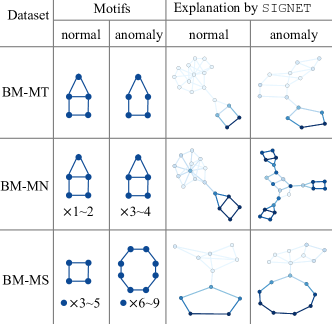
Figure 3: Visualization of explanation results w.r.t. node and edge probabilities.

4.2 Explainability Results (RQ1)

Quantitative evaluation. In Table 1, we report the node-level and edge-level explanation AUC [22] on 6 datasets. Note that PGExplainer [20] can only provide edge-level explanations natively. We have the following observations: 1) SIGNET achieves SOTA performance in almost all scenarios. Compared to the best baselines, the average performance gains of SIGNET are $27.89\%$ in NX-AUC and $8.99\%$ in EX-AUC. The superior performance verifies the significance of learning to interpret and detect with a unified model. 2) The post-hoc explainers are not compatible with all GLAD models. For instance, PGExplainer works relevantly well with GLocalKD but cannot provide informative explanations for OCGIN. The GNNExplainer, unfortunately, exhibits poor performance in most scenarios. 3) SIGNET has larger performance gains on real-world datasets, which illustrates the potential of SIGNET in explaining real-world GLAD tasks. 4) Despite its superior performance, the stability of SIGNET is relevantly average. Especially on the synthetic datasets, we can find that the standard deviations of NX-AUC and EX-AUC are large. We speculate that the instability is due to the lack of labels that provide reliable supervisory signals for anomaly detection explanations.

Qualitative evaluation. To better understand the behavior of SIGNET, we visualize the explanations (i.e., node and edge probabilities) in Fig. 3. We can witness that SIGNET can assign larger probabilities for the nodes and edges within the discriminative motifs, providing valid explanations for the GLAD predictions. In contrast, the probabilities of base subgraphs are uniformly small, indicating that SIGNET is able to ignore the unrelated substructure. However, we can still witness some irrelevant nodes included in the explanations in the anomaly sample of BM-MN dataset, which indicates that SIGNET may generate noisy explanations in some special cases.

4.3 Anomaly Detection Results (RQ2)

To investigate the anomaly detection performance of SIGNET, we conduct experiments on 16 datasets and summarize the results in Table 2. The following observations can be concluded: 1) SIGNET outperforms all baselines on 10 datasets and achieves competitive performance on the rest. The main reason is that SIGNET can capture graph patterns at node and edge level with two distinct views and concentrate on the key substructure during anomaly scoring. 2) The deep GLAD methods generally perform better than kernel-based methods, indicating that GNN-based deep learning models are effective in identifying anomalous graphs. To sum up, SIGNET can not only accurately detect anomalies but also provide informative interpretations for the predictions.

Table 2: Anomaly detection performance in terms of AD-AUC (in percent, mean $\pm$ std). The best and runner-up results are highlighted with bold and underline, respectively.

Dataset	PK-OCSVM	PK-iF	WL-OCSVM	WL-iF	OCGIN	GLocalKD	OCGTL	SIGNET
BM-MT	$52.58{\scriptstyle\pm 0.35}$	$45.30{\scriptstyle\pm 1.60}$	$53.36{\scriptstyle\pm 0.46}$	$50.30{\scriptstyle\pm 0.40}$	$73.33{\scriptstyle\pm 6.18}$	$74.94{\scriptstyle\pm 5.12}$	${\color[rgb]{0.92578125,0.328125,0.15625}\underline{93.61{\scriptstyle\pm 0.20}}}$	${\color[rgb]{0.59765625,0.203125,0.1875}\mathbf{95.89{\scriptstyle\pm 2.75}}}$
BM-MN	${\color[rgb]{0.92578125,0.328125,0.15625}\underline{97.13{\scriptstyle\pm 0.19}}}$	$56.80{\scriptstyle\pm 4.65}$	$76.60{\scriptstyle\pm 0.77}$	$49.90{\scriptstyle\pm 0.20}$	$59.35{\scriptstyle\pm 2.81}$	$77.51{\scriptstyle\pm 3.08}$	${\color[rgb]{0.59765625,0.203125,0.1875}\mathbf{99.49{\scriptstyle\pm 0.05}}}$	$93.41{\scriptstyle\pm 1.66}$
BM-MS	$79.34{\scriptstyle\pm 0.52}$	$57.00{\scriptstyle\pm 6.15}$	$56.19{\scriptstyle\pm 0.42}$	$51.30{\scriptstyle\pm 0.03}$	$58.00{\scriptstyle\pm 3.44}$	$65.03{\scriptstyle\pm 2.36}$	${\color[rgb]{0.92578125,0.328125,0.15625}\underline{92.01{\scriptstyle\pm 0.82}}}$	${\color[rgb]{0.59765625,0.203125,0.1875}\mathbf{94.01{\scriptstyle\pm 4.88}}}$
MNIST-0	$48.89{\scriptstyle\pm 2.19}$	$59.58{\scriptstyle\pm 1.50}$	$67.19{\scriptstyle\pm 2.69}$	$59.27{\scriptstyle\pm 2.43}$	$69.54{\scriptstyle\pm 2.61}$	${\color[rgb]{0.92578125,0.328125,0.15625}\underline{82.29{\scriptstyle\pm 1.65}}}$	$80.68{\scriptstyle\pm 3.14}$	${\color[rgb]{0.59765625,0.203125,0.1875}\mathbf{83.25{\scriptstyle\pm 2.17}}}$
MNIST-1	$43.45{\scriptstyle\pm 1.32}$	$78.97{\scriptstyle\pm 5.54}$	$63.64{\scriptstyle\pm 2.60}$	$65.05{\scriptstyle\pm 3.21}$	${\color[rgb]{0.59765625,0.203125,0.1875}\mathbf{98.25{\scriptstyle\pm 0.61}}}$	$93.04{\scriptstyle\pm 0.65}$	${\color[rgb]{0.92578125,0.328125,0.15625}\underline{97.98{\scriptstyle\pm 0.36}}}$	$90.12{\scriptstyle\pm 5.21}$
MUTAG	$53.30{\scriptstyle\pm 1.29}$	$43.60{\scriptstyle\pm 1.72}$	$49.64{\scriptstyle\pm 2.89}$	$49.07{\scriptstyle\pm 0.32}$	$57.59{\scriptstyle\pm 3.36}$	${\color[rgb]{0.92578125,0.328125,0.15625}\underline{65.09{\scriptstyle\pm 5.94}}}$	$63.41{\scriptstyle\pm 2.60}$	${\color[rgb]{0.59765625,0.203125,0.1875}\mathbf{87.72{\scriptstyle\pm 3.48}}}$
PROTEINS-F	$50.49{\scriptstyle\pm 4.92}$	$60.70{\scriptstyle\pm 2.55}$	$51.35{\scriptstyle\pm 4.35}$	$61.36{\scriptstyle\pm 2.54}$	$70.89{\scriptstyle\pm 2.44}$	${\color[rgb]{0.59765625,0.203125,0.1875}\mathbf{77.30{\scriptstyle\pm 5.15}}}$	${\color[rgb]{0.92578125,0.328125,0.15625}\underline{76.51{\scriptstyle\pm 1.55}}}$	$75.22{\scriptstyle\pm 3.91}$
ENZYMES	$53.67{\scriptstyle\pm 2.66}$	$51.30{\scriptstyle\pm 2.01}$	$55.24{\scriptstyle\pm 2.66}$	$51.60{\scriptstyle\pm 3.81}$	$58.75{\scriptstyle\pm 5.98}$	$61.39{\scriptstyle\pm 8.81}$	${\color[rgb]{0.92578125,0.328125,0.15625}\underline{62.06{\scriptstyle\pm 3.36}}}$	${\color[rgb]{0.59765625,0.203125,0.1875}\mathbf{62.96{\scriptstyle\pm 4.22}}}$
AIDS	$50.79{\scriptstyle\pm 4.30}$	$51.84{\scriptstyle\pm 2.87}$	$50.12{\scriptstyle\pm 3.43}$	$61.13{\scriptstyle\pm 0.71}$	$78.16{\scriptstyle\pm 3.05}$	$93.27{\scriptstyle\pm 4.19}$	${\color[rgb]{0.59765625,0.203125,0.1875}\mathbf{99.40{\scriptstyle\pm 0.57}}}$	${\color[rgb]{0.92578125,0.328125,0.15625}\underline{97.27{\scriptstyle\pm 1.17}}}$
DHFR	$47.91{\scriptstyle\pm 3.76}$	$52.11{\scriptstyle\pm 3.96}$	$50.24{\scriptstyle\pm 3.13}$	$50.29{\scriptstyle\pm 2.77}$	$49.23{\scriptstyle\pm 3.05}$	$56.71{\scriptstyle\pm 3.57}$	${\color[rgb]{0.92578125,0.328125,0.15625}\underline{59.90{\scriptstyle\pm 2.96}}}$	${\color[rgb]{0.59765625,0.203125,0.1875}\mathbf{74.01{\scriptstyle\pm 4.69}}}$
BZR	$46.85{\scriptstyle\pm 5.31}$	$55.32{\scriptstyle\pm 6.18}$	$50.56{\scriptstyle\pm 5.87}$	$52.46{\scriptstyle\pm 3.30}$	$65.91{\scriptstyle\pm 1.47}$	${\color[rgb]{0.92578125,0.328125,0.15625}\underline{69.42{\scriptstyle\pm 7.78}}}$	$63.94{\scriptstyle\pm 8.89}$	${\color[rgb]{0.59765625,0.203125,0.1875}\mathbf{81.44{\scriptstyle\pm 9.23}}}$
COX2	$50.27{\scriptstyle\pm 7.91}$	$50.05{\scriptstyle\pm 2.06}$	$49.86{\scriptstyle\pm 7.43}$	$50.27{\scriptstyle\pm 0.34}$	$53.58{\scriptstyle\pm 5.05}$	${\color[rgb]{0.92578125,0.328125,0.15625}\underline{59.37{\scriptstyle\pm 12.67}}}$	$55.23{\scriptstyle\pm 5.68}$	${\color[rgb]{0.59765625,0.203125,0.1875}\mathbf{71.46{\scriptstyle\pm 4.64}}}$
DD	$48.30{\scriptstyle\pm 3.98}$	$71.32{\scriptstyle\pm 2.41}$	$47.99{\scriptstyle\pm 4.09}$	$70.31{\scriptstyle\pm 1.09}$	$72.27{\scriptstyle\pm 1.83}$	${\color[rgb]{0.59765625,0.203125,0.1875}\mathbf{80.12{\scriptstyle\pm 5.24}}}$	${\color[rgb]{0.92578125,0.328125,0.15625}\underline{79.48{\scriptstyle\pm 2.02}}}$	$72.72{\scriptstyle\pm 3.91}$
NCI1	$49.90{\scriptstyle\pm 1.18}$	$50.58{\scriptstyle\pm 1.38}$	$50.63{\scriptstyle\pm 1.22}$	$50.74{\scriptstyle\pm 1.70}$	$71.98{\scriptstyle\pm 1.21}$	$68.48{\scriptstyle\pm 2.39}$	${\color[rgb]{0.92578125,0.328125,0.15625}\underline{73.44{\scriptstyle\pm 0.97}}}$	${\color[rgb]{0.59765625,0.203125,0.1875}\mathbf{74.89{\scriptstyle\pm 2.07}}}$
IMDB-B	$50.75{\scriptstyle\pm 3.10}$	$50.80{\scriptstyle\pm 3.17}$	$54.08{\scriptstyle\pm 5.19}$	$50.20{\scriptstyle\pm 0.40}$	$60.19{\scriptstyle\pm 8.90}$	$52.09{\scriptstyle\pm 3.41}$	${\color[rgb]{0.92578125,0.328125,0.15625}\underline{64.05{\scriptstyle\pm 3.32}}}$	${\color[rgb]{0.59765625,0.203125,0.1875}\mathbf{66.48{\scriptstyle\pm 3.49}}}$
REDDIT-B	$45.68{\scriptstyle\pm 2.24}$	$46.72{\scriptstyle\pm 3.42}$	$49.31{\scriptstyle\pm 2.33}$	$48.26{\scriptstyle\pm 0.32}$	$75.93{\scriptstyle\pm 8.65}$	$77.85{\scriptstyle\pm 2.62}$	${\color[rgb]{0.59765625,0.203125,0.1875}\mathbf{86.81{\scriptstyle\pm 2.10}}}$	${\color[rgb]{0.92578125,0.328125,0.15625}\underline{82.78{\scriptstyle\pm 1.11}}}$
Avg. Rank	$6.6$	$6.1$	$6.2$	$6.4$	$4.1$	$2.8$	${\color[rgb]{0.92578125,0.328125,0.15625}\underline{2.1}}$	${\color[rgb]{0.59765625,0.203125,0.1875}\mathbf{1.7}}$

4.4 Ablation Study (RQ3)

Table 3: Performance of SIGNET and its variants.

Variant	BM-MS			MNIST-0
	NX-AUC	EX-AUC	AD-AUC	NX-AUC	EX-AUC	AD-AUC
Aug. View	$66.87$	$64.48$	$63.26$	$41.82$	$39.25$	$48.75$
Str. View	$70.36$	$68.27$	$92.79$	$51.73$	$50.40$	$55.29$
2E w $D_{SKL}$	$70.71$	$65.23$	$92.44$	$59.22$	$57.33$	$81.77$
2E w/o $D_{SKL}$	$73.54$	$37.15$	$87.84$	$57.92$	$43.65$	$80.97$
JS MI Est.	$70.35$	$68.96$	$75.21$	$59.06$	$63.85$	$71.78$
DV MI Est.	$72.53$	$74.16$	$74.87$	$60.90$	$70.28$	$70.31$
SIGNET	$76.42$	$79.48$	$94.01$	$70.38$	$72.78$	$83.25$

We perform ablation studies to evaluate the effectiveness of core designs in SIGNET, i.e., dual hypergraph-based view construction, single extractor, and InfoNCE MI estimator. We replace these components with alternative designs, and the results are illustrated in Table 3. We consider two strategies for view construction: augmentation-based view construction [46] (Aug. View) and structural property-based view construction [50] (Str. View). As we discussed in Sec. 3.2, perturbation-based graph augmentation is not appropriate for GLAD tasks, leading to its poor performance. The structural property-based strategy has better performance on BM-BT but still performs weakly on MNIST-0. In contrast, dual hypergraph-based view construction is a better strategy that jointly considers node-level and edge-level information, contributing to optimal detection and explanation performance. We also test the performance of SIGNET with two extractors (2E) and discuss the contribution of SKL divergence. We can find that even with the help of $D_{SKL}$, the two-extractor version still underperforms the original SIGNET with one extractor. Meanwhile, we can witness that compared to JS [54] and DV [55] MI estimators, Info-NCE estimator can lead to superior performance, especially for anomaly detection.

5 Conclusion

This paper presents a novel and practical research problem, explainable graph-level anomaly detection (GLAD). Based on the information bottleneck principle, we deduce the framework multi-view subgraph information bottleneck (MSIB) to address the explainable GLAD problem. We develop a new method termed SIGNET by instantiating MSIB framework with advanced neural modules. Extensive experiments verify the effectiveness of SIGNET in identifying anomalies and providing explanations. A limitation of our paper is that we mainly focus on purely unsupervised GLAD scenarios where ground-truth labels are entirely unavailable. As a result, for few-shot or semi-supervised GLAD scenarios [44] where a few labels are accessible, SIGNET cannot directly leverage them for model training and self-interpretation. We leave the exploration of supervised/semi-supervised self-interpretable GLAD problems in future works.

Appendix A Definitions of “Explainability” and “Interpretability”

Since explainable artificial intelligence is an emerging area of research, how to specifically discriminate similar concepts “explainability” and “interpretability” is not yet completely standardized. Following the recent survey paper [18], we distinguish them with definite principles rather than using them interchangeably.

Specifically, we define the term “explainability” as a more general and high-level concept that includes all learning scenarios, models, and strategies related to providing understandable knowledge for the predictions. The major reason is that “explainable artificial intelligence” and “explainable machine learning” are well-known concepts in the community. For instance, we denote the ability to explain GNNs’ predictions as “explainability of GNNs”, and the related learning tasks include explainable node classification, explainable graph classification, etc. Following this way, we denote our proposed learning problem as “explainable graph-level anomaly detection (GLAD)”.

Differently, we denote “interpretability” as the ability of a model to intrinsically provide explanations for itself. To well emphasis the characteristic of interpreting itself, we sometimes use the concept “self-interpretability” interchangeably with the concept “interpretability”. For instance, the GNNs that can jointly generate predictions and explanations are denoted as “interpretable GNNs” or “self-interpretable GNNs”. Under such a definition, the models that provide post-hoc explanations for trained GNNs are not interpretable. In this paper, we aim to propose a “self-interpretable GLAD model” that is able to yield explanations for the anomaly detection results by itself.

Appendix B Related Work in Detail

Graph Neural Networks (GNNs). GNNs are the extension of the convolution-based neural networks onto graph data [1, 2, 23, 24, 26, 27, 66, 67]. Early GNNs define graph convolution based on spectral theory [66, 68]. Recently, the mainstream GNNs usually follow the paradigm of message passing for spatial graph convolution, i.e., executing graph convolution by aggregating the information for adjacent nodes [2, 23, 24, 26]. For instance, GCN [23] uses an average-based aggregation function for message passing. GIN [2], differently, employs a summation-based aggregation function to ensure its expressive ability. Apart from normal GNNs designed for simple graphs where each edge connects exactly two nodes, some recent studies apply GNNs to hypergraphs, a generalization of graphs where an edge can connect more than two nodes [29, 30, 31]. Among them, Hyper-Conv [30] is a representative HGNN that applies a GCN-like aggregation function to the graph convolution for hypergraphs. Thanks to their strong expressive power, GNNs are effective in various graph learning tasks, such as node classification [23, 69, 70, 71], graph classification [2], and also graph anomaly detection [25, 72]. Besides, GNNs can also be widely applied to diverse real-world learning scenarios, such as federated learning [73, 74], knowledge graph reasoning [75, 76, 77], adversarial attack [78, 79], and molecule analysis [46, 80].

Explainability of GNNs. To make the predictions of GNNs transparent and understandable, a line of studies proposes to uncover the explanation, i.e., the critical subgraphs and/or features that highly correlate to the prediction, for GNN models [18, 19, 20, 21, 33, 32]. Existing methods can be divided into two types: post-hoc GNN explainer and self-interpretable GNN [21, 32]. The post-hoc GNN explainers use specialized models or strategies to explain the behavior of a trained GNN, such as input perturbation [19, 20], surrogate model [33], and prediction decomposition [81]. For instance, PGExplainer [20] uses an edge embedding-based neural module to modify the input graph, and the learning objective is to optimize the cross-entropy between the original prediction and the modified input. Differently, the self-interpretable GNNs can intrinsically provide explanations for the predictions using the interpretable designs in GNN architectures [13, 21, 22]. GSAT [22] is one of the self-interpretable GNNs that uses a parameterized attention module to pick the graph rationale along with the training of the GNN backbone. Theoretically, the post-hoc explainers can be used to explain the well-trained GLAD models; however, the post-hoc explainers can potentially provide sub-optimal solutions since they are not directly learned with the detection models. On the other hand, most self-interpretable GNNs are designed to explain the prediction of supervised tasks, especially graph/node classification tasks. In this case, it is non-trivial to directly apply them to unsupervised graph anomaly detection tasks, since their inherent supervised learning objective cannot work without ground-truth labels.

Graph Anomaly Detection. The objective of graph anomaly detection is to identify anomalies that deviate from the majority of samples in graph-structured data [7, 25, 82]. Most efforts mainly focus on node-level anomaly detection, i.e., detecting the abnormal nodes from one or more graphs [25, 72, 83, 84]. In this paper, we mainly investigate graph-level anomaly detection (GLAD) that aims to recognize anomalous graphs from a set of graphs [7, 4, 8, 9]. A few recent studies try to address the GLAD problem with various advanced techniques. For example, OCGIN [7] combines the objective of one-class classification and a GIN encoder into the first GLAD model. GLocalKD [4] uses the knowledge distillation error between a random network and a trainable network to evaluate the abnormality of graph samples. OCGTL [8] introduces a graph transformation learning-based learning objective to identify the anomalous samples in a graph set. However, these methods can only predict the scores to indicate the degree of abnormality of each sample, but cannot provide the behind explanations, i.e., the substructure causes the abnormality. To boost the reliability and explainability of GAD methods, in this paper, we propose a self-interpretable GAD framework to generate both anomaly prediction and its explanation.

Learning by Information-Bottleneck (IB). IB is an information theory-based approach for representation learning that trains the encoder by preserving the information that is relevant to label prediction while minimizing the amount of superfluous information [34, 35, 36]. Formally, the objective of IB principle is to maximize the mutual information (MI) between representation ${Z}$ and label ${Y}$, and minimize the MI between representation ${Z}$ and original data ${X}$ [36]. Some pioneering efforts [37, 85] extend IB principle to multi-view learning scenarios, and some of them enable the application of IB principle for unsupervised learning [37]. Recent efforts also attempt to apply IB principle to graph learning tasks [17, 22, 38, 39, 40, 41, 42, 43]. One feasible idea is to borrow the representation-based IB principle for graph representation learning [39, 42]; another line of work regards a vital bottleneck subgraph ${G}^{(s)}$ rather than the representation ${Z}$ as the bottleneck and tries to maximize the MI between ${G}^{(s)}$ and label ${Y}$ while minimizing the MI between ${G}^{(s)}$ and original graph ${G}$ [17, 40, 41].

Explainable anomaly detection. Anomaly detection is an essential machine learning task that aims to detect unusual or rare patterns or instances within a dataset [11, 86]. In order to improve the trustworthiness and comprehensibility of anomaly detection systems, a brunch of research termed explainable anomaly detection focuses on generating valid explanations for the results given by anomaly detection models [10, 15, 16]. For example, to provide explanations for one-class image anomaly detection models, FCDD [10] uses a fully convolutional module to generate pixel-level explanation. ATON [15] utilizes an attention-guided triplet deviation mechanism to provide explanations for any black-box outlier detector on tabular data. Cho et al. [16] introduce an auxiliary prototypical classifier to learn explanations of anomaly detection models for medical images. Despite their success, these techniques cannot be directly applied to graph-structured data.

Appendix C Formulations of GNN and HGNN

In this section, we provide detailed definitions of message passing-based graph neural network (GNN) and hypergraph neural network (HGNN). Given a simple graph $G$, the target of a GNN is to learn the node-level representation following the message passing scheme:

$$\mathbf{h}_{v}^{(l+1)}=\operatorname{UPDATE}\left(\mathbf{h}_{v}^{(l)},\operatorname{AGGREGATE}\left(\left\{\mathbf{h}_{u}^{(l)}:\forall u\in\mathcal{N}(v;\mathbf{A})\right\}\right)\right),$$ (6)

where $\mathbf{h}_{v}^{(l)}$ is the latent representation vector for node $v\in\mathcal{V}$ at the $l$-th layer (with $\mathbf{h}_{v}^{(0)}=\mathbf{x}_{v}=\mathbf{X}_{[v]}$), $\mathcal{N}(v;\mathbf{A})$ is the neighboring node set of $v$ obtained from $\mathbf{A}$, $\operatorname{AGGREGATE}(\cdot)$ is is the function that aggregates messages from neighboring nodes, and $\operatorname{UPDATE}(\cdot)$ is the function that updates the node representation. With similar notations, we can formulate a HGNN as:

$$\mathbf{h}_{v^{*}}^{(l+1)}=\operatorname{UPDATE}\left(\mathbf{h}_{v^{*}}^{(l)},\operatorname{AGGREGATE}\left(\left\{\mathbf{h}_{u^{*}}^{(l)}:\forall{u^{*}}\in\mathcal{N}({v^{*}};\mathbf{M}^{*})\right\}\right)\right),$$ (7)

where $\mathcal{N}({v^{*}};\mathbf{M}^{*})$ is the neighboring node set of $v^{*}\in\mathcal{V}^{*}$ obtained from incidence matrix $\mathbf{M}^{*}$.

In GNNs, a pooling operation $\operatorname{POOL}(\cdot)$ can be applied to obtain a graph-level representation vector with $\mathbf{h}_{G}=\operatorname{POOL}\left(\{\mathbf{h}_{v}^{(L)}:\forall{v}\in\mathcal{V}\}\right)$ by summarizing the representations of all nodes at the final layer $L$. A similar pooling layer can be used to obtain hypergraph-level representation $\mathbf{h}_{G}^{*}$.

Appendix D MSIB Loss Computation

Starting from Eq. (2), we can first rewrite the objective of the first graph view $G^{1}$ as a loss function into:

$$\mathcal{L}_{1}=I(G^{1};G^{1(s)}|G^{2})-\frac{1}{\beta_{1}}I(G^{2};G^{1(s)}),$$ (8)

which we aim to minimize during model training. Similar to Eq. (8), the corresponding loss function for the second graph view $G^{2}$ can be written by:

$$\mathcal{L}_{2}=I(G^{2};G^{2(s)}|G^{1})-\frac{1}{\beta_{2}}I(G^{1};G^{2(s)}),$$ (9)

where $\beta_{2}$ is the trade-off parameter for $\mathcal{L}_{2}$. Then, by computing the average of $\mathcal{L}_{1}$ and $\mathcal{L}_{2}$, we have a joint loss function to optimize both $G^{1(s)}$ and $G^{2(s)}$:

$$\mathcal{L}_{joint}=\frac{I(G^{1};G^{1(s)}|G^{2})+I(G^{2};G^{2(s)}|G^{1})}{2}-\frac{\frac{1}{\beta_{1}}I(G^{2};G^{1(s)})+\frac{1}{\beta_{2}}I(G^{1};G^{2(s)})}{2}.$$ (10)

For term $I(G^{1};G^{1(s)}|G^{2})$, we can derive its upper bound by:

$$I_{\theta}\left(G^{1};G^{1(s)}|G^{2}\right)=\mathbb{E}_{\boldsymbol{G}^{1},\boldsymbol{G}^{2}\sim p\left(G^{1},G^{2}\right)}\mathbb{E}_{\boldsymbol{G}^{(s)}\sim p_{\theta}\left(G^{1(s)}|G^{1}\right)}\left[\log\frac{p_{\theta}\left(G^{1(s)}=\boldsymbol{G}^{(s)}|G^{1}=\boldsymbol{G}^{1}\right)}{p_{\theta}\left(G^{1(s)}=\boldsymbol{G}^{(s)}|G^{2}=\boldsymbol{G}^{2}\right)}\right]$$ (11)

$$=\mathbb{E}_{\boldsymbol{G}^{1},\boldsymbol{G}^{2}\sim p\left(G^{1},G^{2}\right)}\mathbb{E}_{\boldsymbol{G}^{(s)}\sim p_{\theta}\left(G^{1(s)}|G^{1}\right)}\left[\log\frac{p_{\theta}\left(G^{1(s)}=\boldsymbol{G}^{(s)}|G^{1}=\boldsymbol{G}^{1}\right)}{p_{\psi}\left(G^{2(s)}=\boldsymbol{G}^{(s)}|G^{2}=\boldsymbol{G}^{2}\right)}\frac{p_{\psi}\left(G^{2(s)}=\boldsymbol{G}^{(s)}|G^{2}=\boldsymbol{G}^{2}\right)}{p_{\theta}\left(G^{1(s)}=\boldsymbol{G}^{(s)}|G^{2}=\boldsymbol{G}^{2}\right)}\right]$$

$$=D_{KL}\left(p_{\theta}(G^{1(s)}|G^{1})\|p_{\psi}(G^{2(s)}|G^{2}\right))-D_{KL}\left(p_{\theta}(G^{2(s)}|G^{1})||p_{\psi}(G^{2(s)}|G^{2})\right)$$

$$\leq D_{KL}\left(p_{\theta}(G^{1(s)}|G^{1})\|p_{\psi}(G^{2(s)}|G^{2})\right).$$

where $D_{KL}(\cdot)$ is the Kullback–Leibler (KL) divergence. Analogously, we can acquire the upper bound of $I(G^{2};G^{2(s)}|G^{1})$ as $D_{KL}\left(p_{\theta}(G^{2(s)}|G^{2})\|p_{\psi}(G^{1(s)}|G^{1})\right)$. In this way, the first term in Eq. (10) can be upperbound by:

$$\frac{I(G^{1};G^{1(s)}|G^{2})+I(G^{2};G^{2(s)}|G^{1})}{2}\leq D_{SKL}\left(p_{\theta}(G^{1(s)}|G^{1})\|p_{\psi}(G^{2(s)}|G^{2})\right),$$ (12)

where $D_{SKL}\left(p_{\theta}(G^{1(s)}|G^{1})\|p_{\psi}(G^{2(s)}|G^{2})\right)=\frac{1}{2}D_{KL}\left(p_{\theta}(G^{1(s)}|G^{1})\|p_{\psi}(G^{2(s)}|G^{2})\right)+\frac{1}{2}D_{KL}\left(p_{\theta}(G^{2(s)}|G^{2})\|p_{\psi}(G^{1(s)}|G^{1})\right)$.

Then, according to the chain rule of mutual information, i.e., $I(xy;z)=I(y;z)+I(x;z|y)$, we can reform the term $I(G^{2};G^{1(s)})$ by:

$$I(G^{1(s)};G^{2}) =I(G^{1(s)};G^{2(s)}G^{2})-I(G^{1(s)};G^{2(s)}|G^{2})$$ (13)

$$\stackrel{{\scriptstyle(H)}}{{=}}I(G^{1(s)};G^{2(s)}G^{2})$$

$$=I(G^{1(s)};G^{2(s)})+I(G^{1(s)};G^{2}|G^{2(s)})$$

$$\geq I(G^{1(s)};G^{2(s)}),$$

where $(H)$ indicates the hypothesis that $G^{2(s)}$ is sufficient for $G^{1}$, i.e., $I(G^{1(s)};G^{2(s)}|G^{1})$ = 0. Symmetrically, we can also have $I(G^{2(s)};G^{1})\geq I(G^{1(s)};G^{2(s)})$. In this case, the second term in Eq. (10) has the lower bound with:

$$\frac{\frac{1}{\beta_{1}}I(G^{2};G^{1(s)})+\frac{1}{\beta_{2}}I(G^{1};G^{2(s)})}{2}\geq\frac{(\beta_{1}+\beta_{2})}{2\beta_{1}\beta_{2}}I(G^{1(s)};G^{2(s)}).$$ (14)

By jointly considering Eq. (12) and Eq. (14), the joint loss function (Eq. (10)) can be bounded by:

$$\mathcal{L}_{joint}\leq D_{SKL}\left(p_{\theta}(G^{1(s)}|G^{1})\|p_{\psi}(G^{2(s)}|G^{2})\right)-\frac{(\beta_{1}+\beta_{2})}{2\beta_{1}\beta_{2}}I(G^{1(s)};G^{2(s)}).$$ (15)

Finally, by multiplying both terms with $\beta=\frac{2\beta_{1}\beta_{2}}{(\beta_{1}+\beta_{2})}$ and re-parametrizing the objective, we have a tractable loss function for MSIB framework:

$$\mathcal{L}_{MSIB}=-I(G^{1(s)};G^{2(s)})+\beta D_{SKL}\left(p_{\theta}(G^{1(s)}|G^{1})\|p_{\psi}(G^{2(s)}|G^{2})\right).$$ (16)

Appendix E Methodology Discussion

Input: Training Set $\mathcal{G}_{tr}$; Test Set $\mathcal{G}_{te}$.

Parameters : Number of epoch $E$.

Output: Anomaly Score Set $\mathcal{S}$; Explanation Subgraph Set $\mathcal{G}^{(es)}$.

/* Training */

1 Initialize model parameters

2 for $e=1,2,\cdots,E$ do

3       $\mathcal{B}_{1},\cdots,\mathcal{B}_{n_{b}}$ $\leftarrow$ Randomly split $\mathcal{G}_{tr}$ into batches

4       for $\mathcal{B}=\mathcal{B}_{1},\cdots,\mathcal{B}_{n_{b}}$ do

5             for $G_{i}\in\mathcal{B}$ do

6                   $G_{i}^{*}\leftarrow$ Obtain the dual hypergraph of $G_{i}$ by DHT

7                   $\mathbf{p}_{i},\mathbf{p}^{*}_{i}\leftarrow$ Calculate probability vectors by neural extractor

8                   $G_{i}^{(s)},G_{i}^{*(s)}\leftarrow$ Extract bottleneck subgraphs by Eq. (4)

9                   $\mathbf{h}_{i}^{(s)},\mathbf{h}_{i}^{*(s)}\leftarrow$ Calculate graph-level representations by GNN/HGNN encoders

10                  

11             end for

12            $\mathcal{L}\leftarrow$ Calculate Info-NCE loss by Eq. (5)

13             Update model parameters via gradient descent w.r.t. $\mathcal{L}$

14            

15       end for

16      

17 end for

/* Inference */

18 for $G_{i}\in\mathcal{G}_{te}$ do

19       $G_{i}^{*}\leftarrow$ Obtain the dual hypergraph of $G_{i}$ by DHT

20       $\mathbf{p}_{i},\mathbf{p}^{*}_{i}\leftarrow$ Calculate probability vectors by neural extractor

21       $G_{i}^{(s)},G_{i}^{*(s)}\leftarrow$ Extract bottleneck subgraphs by Eq. (4)

22       $\mathbf{h}_{i}^{(s)},\mathbf{h}_{i}^{*(s)}\leftarrow$ Calculate graph-level representations by GNN/HGNN encoders

23       $s_{i}=-I(\mathbf{h}_{i}^{(s)},\mathbf{h}_{i}^{*(s)})\leftarrow$ Calculate the anomaly score of $G_{i}$ by Info-NCE MI estimator

24       $G^{(es)}_{i}\leftarrow$ Extract explanation subgraph according to $\mathbf{p}_{i}$ and $\mathbf{p}^{*}_{i}$ using top-k/threshold strategy

25 end for

$\mathcal{S},\mathcal{G}^{(es)}\leftarrow$ Collect all the anomaly scores $s_{i}$ and explanations $G^{(es)}_{i}$ into sets

Algorithm 1 The overall algorithm of SIGNET

E.1 Algorithm

The overall algorithm of SIGNET is summarized in Algo. 1.

E.2 Discussion of SIGNET v.s. GSAT

In this paragraph, we discuss the connections and differences between SIGNET and the representative self-interpretable GNNs, GSAT.

Connections between SIGNET and GSAT:

• Theoretical foundation. Both GSAT and SIGNET are based on the well-known information theory criteria, the information bottleneck, serving as their theoretical foundation for their explanation target.

• Explanation goal. As an explainable method for graphs, they have a common objective of identifying the key subgraph within the input graph sample that holds the highest relevance to the final prediction.

• Architecture. Both GSAT and SIGNET adopt learnable neural networks to parameterize the graph data and make the explanation differentiable, which is a common design among explainable GNNs. However, GSAT only conducts the relaxation at the edge level, while SIGNET can provide explanation scores at both node and edge levels.

Differences between SIGNET and GSAT:

• Targeted tasks. GSAT focuses on a supervised graph-level classification task where categorical labels are available for training the self-interpretation module. On the other hand, SIGNET targets unsupervised graph-level anomaly detection, a more challenging task with unavailable labels during training.

• Theoretical framework. GSAT is designed based on the original information bottleneck framework with subgraph bottleneck, tailored to its targeted supervised setting. In contrast, SIGNET is based on the multi-view subgraph information bottleneck (MSIB) framework derived in this paper, specifically designed for unsupervised anomaly detection tasks.

• Learning objectives. GSAT is trained using cross-entropy loss, a commonly used classification loss. In contrast, SIGNET is optimized using an Info-NCE loss, aiming to maximize the mutual information between each graph and its rational subgraph.

• Graph view for learning. GSAT only considers the original view for graph learning, while SIGNET takes both the original and DHT views into account for self-interpretable graph learning.

E.3 Complexity analysis

Within this paragraph, we denote the average numbers of nodes and edges as $n$ and $m$ respectively, and denote the number of graphs and batch size as $N$ and $B$ respectively. At each training iteration, we first conduct DHT to obtain the dual hypergraph, which requires $\mathcal{O}(N(m+n))$. Then, the GNN-based extractor that calculates probability consumes $\mathcal{O}(NL_{1}md_{1}+NL_{1}nd_{1}^{2}+Nnd_{1}d_{f})$ complexity, where $L_{1}$ and $d_{1}$ are the layer number and latent dimension of the extractor, respectively. The bottleneck subgraph extraction for two views requires $\mathcal{O}(N(m+n))$ in total. For the GNN and HGNN encoders, their time complexities are $\mathcal{O}(NL_{2}md_{2}+NL_{2}nd_{2}^{2}+Nnd_{2}d_{f})$ and $\mathcal{O}(NL_{2}nd_{2}+NL_{2}md_{2}^{2}+Nnd_{2}d_{f*})$ respectively, where $L_{2}$ and $d_{2}$ denote their layer number and latent dimension. Finally, the Info-NCE loss requires $\mathcal{O}(NBd_{2})$ complexity. To simplify the overall complexity, we denote the larger terms within $L_{1}$ and $L_{2}$ as $L$, and the larger terms between $d_{1}$ and $d_{2}$ as $d$. After ignoring the smaller terms, the overall complexity of SIGNET is $\mathcal{O}(NLd^{2}(m+n)+Nnd(d_{f}+d_{f*})+NBd)$.

Appendix F Supplement of Experimental Setup

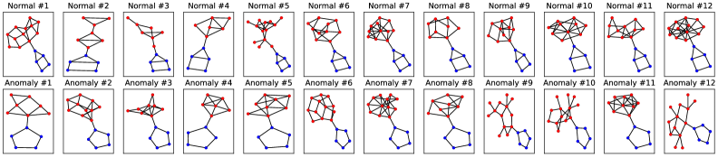
(a) BM-MT

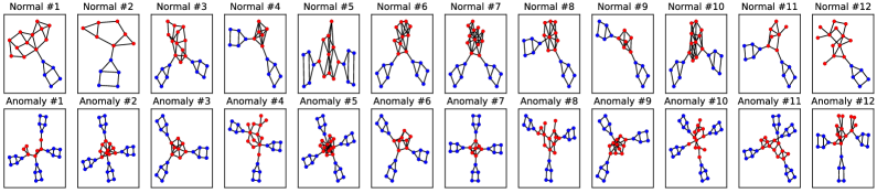
(b) BM-MN

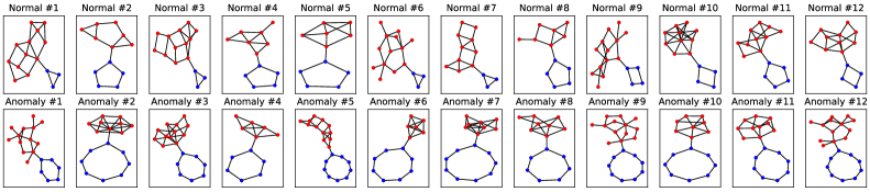
(c) BM-MS

Figure 4: Examples of three synthetic datasets, where subgraphs in blue are the ground-truth explanations.

F.1 Datasets

We consider 16 benchmark datasets in total. The statistic of the datasets is provided in Table 4. In this paper, we take “PROTEINS-F”, “IMDB-B”, and “REDDIT-B” as the abbreviations of “PROTEIN-full”, “IMDB-BINARY”, and “REDDIT-BINARY”, respectively. For our synthetic datasets, we provide some examples in Fig. 4.

Table 4: Statistics of datasets.

Dataset	# Graphs (Train/Test)	# Nodes (avg.)	# Edges (avg.)
BM-MT	500/200	14.3	44.5
BM-MN	500/200	18.4	56.7
BM-MS	500/200	14.0	42.8
MNIST-0	1000/500	69.4	572.2
MNIST-1	1000/500	57.9	419.6
MUTAG	1742/295	30.1	60.9
PROTEINS-F	360/223	39.1	72.8
ENZYMES	400/120	32.6	62.1
AIDS	1280/400	15.7	16.2
DHFR	368/152	42.4	44.5
BZR	69/81	35.8	38.4
COX2	81/94	41.2	43.5
DD	390/236	284.3	715.7
NCI1	1646/822	29.8	32.3
IMDB-B	400/200	19.8	96.5
REDDIT-B	800/400	429.6	497.8

F.2 Hyper-parameters

We select the key hyper-parameters of SIGNET through a group-level grid search. Specifically, the hyper-parameters for each benchmark dataset are demonstrated in Table 5. Note that for the dataset without ground-truth explanations, we would not tune the hyper-parameters for the subgraph extractor but use the default ones. The grid search is carried out on the following search space:

• Number of epochs $E$: {10, 50, 100, 200, 500, 800, 1000}

• Learning rate ${lr}$: {1e-2, 1e-3, 1e-4}

• Layer number of encoders $L_{enc}$: {2,3,4,5}

• Hidden dimension of encoders $D_{enc}$: {16,32,64,128}

• Model type of subgraph extractor $EXT$: {MLP,GIN}

• Layer number of subgraph extractor $L_{ext}$: {2,3,4,5}

• Hidden dimension of subgraph extractor $D_{ext}$: {4,8,16,32}

To ensure robust and reliable results, we also conducted a comprehensive grid search to obtain the best hyperparameter configurations for the baselines. Specifically, for deep GLAD methods (i.e., OCGIN, GLocalKD, and OCGTL), we performed grid searches on both general hyperparameters (e.g., layer number and hidden dimensions) and model-specific hyperparameters (e.g., the number of transformations in OCGTL). Similarly, for post-hoc explainers, we conducted grid searches on their post-hoc training iterations and learning rates. As for shallow GLAD methods, we focused on searching for key hyperparameters such as the training iterations of detectors and kernel-specific parameters.

Table 5: Details of the hyper-parameters tuned by grid search.

Dataset	$E$	$lr$	$L_{enc}$	$D_{enc}$	$EXT$	$L_{ext}$	$D_{ext}$
BM-MT	1000	1e-2	5	16	GNN	2	16
BM-MN	500	1e-2	5	16	GNN	3	8
BM-MS	200	1e-2	5	16	GNN	2	32
MNIST-0	50	1e-2	2	16	MLP	2	16
MNIST-1	50	1e-2	2	16	MLP	2	16
MUTAG	50	1e-2	5	16	GNN	5	4
PROTEINS-F	800	1e-3	5	16	GNN	5	8
ENZYMES	1000	1e-3	5	128	GNN	5	8
AIDS	1000	1e-4	5	16	GNN	5	8
DHFR	1000	1e-4	5	128	GNN	5	8
BZR	1000	1e-4	5	128	GNN	5	8
COX2	1000	1e-4	5	64	GNN	5	8
DD	100	1e-4	5	128	GNN	5	8
NCI1	1000	1e-4	5	128	GNN	5	8
IMDB-B	10	1e-4	5	64	GNN	5	8
REDDIT-B	1000	1e-4	5	128	GNN	5	8

F.3 Metrics for explanation performance evaluation

We tackle the explanation problem by framing it as a binary classification task for nodes and edges. We designate nodes and edges inside the explanation subgraph as positive instances and the rest as negative. The importance weights generated by the explanation methods serve as prediction scores. An effective explanation method should assign higher weights to nodes and edges within the ground truth subgraphs compared to those outside. To quantitatively evaluate the performance, we use the AUC as the metric for this binary classification problem. A higher AUC indicates better performance in providing meaningful explanations.

F.4 Implementation of GLAD methods with post-hoc explainers

Given a GLAD model and post-hoc explainer, at first, we train the GLAD model independently on the training set. After sufficient training, the GLAD model is able to map each input graph into a scalar, i.e., its anomaly score. To address the uncertainty of the anomaly score boundaries, we apply a linear scaling function to map the scores into the [0,1] range and then use a sigmoid function to convert each score into a probability for binary classification. Subsequently, we integrate the post-hoc explainer with the probabilized output of the GLAD model and optimize the explainer accordingly.

F.5 Computing infrastructures

We implement the proposed SIGNET with PyTorch 1.12.0 [87] and PyTorch Geometric (PyG) 2.3.0 [88]. The experiments are conducted on a Linux server with an Intel Xeon E-2288G CPU and two Quadro RTX 6000 GPUs.

Appendix G Further Supplementary of Qualitative Experiments

More visualization of explanation results by SIGNET are given in Fig. 5. In specific, we visualize the node-level and edge-level probabilities on four datasets, i.e., BM-MT, BM-MN, BM-MS, and MUTAG. For each dataset, the top row includes 5 normal examples, and the bottom row includes 5 anomalous examples. For MUTAG dataset, the normal examples do not have a specific rationale, while the rationales for anomalies are -NO2 or -NH2.

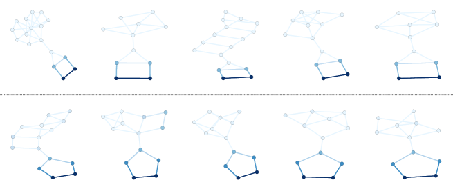
(a) BM-MT

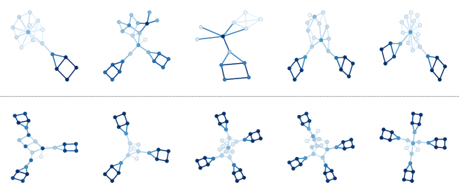
(b) BM-MN

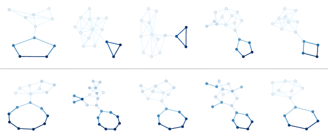
(c) BM-MS

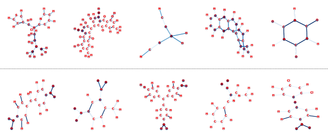
(d) MUTAG

Figure 5: Visualization of explanation results w.r.t. node and edge probabilities. For each dataset, the top row includes 5 normal examples, and the bottom row includes 5 anomalous examples.

References

- [1] Zonghan Wu, Shirui Pan, Fengwen Chen, Guodong Long, Chengqi Zhang, and S Yu Philip. A comprehensive survey on graph neural networks. IEEE transactions on neural networks and learning systems, 32(1):4–24, 2020.
- [2] Keyulu Xu, Weihua Hu, Jure Leskovec, and Stefanie Jegelka. How powerful are graph neural networks? In International Conference on Learning Representations, 2019.
- [3] Xin Zheng, Yixin Liu, Zhifeng Bao, Meng Fang, Xia Hu, Alan Wee-Chung Liew, and Shirui Pan. Towards data-centric graph machine learning: Review and outlook. arXiv preprint arXiv:2309.10979, 2023.
- [4] Rongrong Ma, Guansong Pang, Ling Chen, and Anton van den Hengel. Deep graph-level anomaly detection by glocal knowledge distillation. In Proceedings of the Fifteenth ACM International Conference on Web Search and Data Mining, pages 704–714, 2022.
- [5] Charu C Aggarwal and Haixun Wang. Graph data management and mining: A survey of algorithms and applications. Managing and mining graph data, pages 13–68, 2010.
- [6] Tommaso Lanciano, Francesco Bonchi, and Aristides Gionis. Explainable classification of brain networks via contrast subgraphs. In Proceedings of the 26th ACM SIGKDD International Conference on Knowledge Discovery & Data Mining, pages 3308–3318, 2020.
- [7] Lingxiao Zhao and Leman Akoglu. On using classification datasets to evaluate graph outlier detection: Peculiar observations and new insights. Big Data, 2021.
- [8] Chen Qiu, Marius Kloft, Stephan Mandt, and Maja Rudolph. Raising the bar in graph-level anomaly detection. In Proceedings of the Thirty-First International Joint Conference on Artificial Intelligence, IJCAI-22, pages 2196–2203, 7 2022.
- [9] Xuexiong Luo, Jia Wu, Jian Yang, Shan Xue, Hao Peng, Chuan Zhou, Hongyang Chen, Zhao Li, and Quan Z Sheng. Deep graph level anomaly detection with contrastive learning. Scientific Reports, 12(1):19867, 2022.
- [10] Philipp Liznerski, Lukas Ruff, Robert A Vandermeulen, Billy Joe Franks, Marius Kloft, and Klaus Robert Muller. Explainable deep one-class classification. In International Conference on Learning Representations, 2021.
- [11] Suseela T Sarasamma, Qiuming A Zhu, and Julie Huff. Hierarchical kohonenen net for anomaly detection in network security. IEEE Transactions on Systems, Man, and Cybernetics, Part B (Cybernetics), 35(2):302–312, 2005.
- [12] Grégoire Montavon, Wojciech Samek, and Klaus-Robert Müller. Methods for interpreting and understanding deep neural networks. Digital signal processing, 73:1–15, 2018.
- [13] Yingxin Wu, Xiang Wang, An Zhang, Xiangnan He, and Tat-Seng Chua. Discovering invariant rationales for graph neural networks. In International Conference on Learning Representations, 2022.
- [14] Sihang Li, Xiang Wang, An Zhang, Yingxin Wu, Xiangnan He, and Tat-Seng Chua. Let invariant rationale discovery inspire graph contrastive learning. In International Conference on Machine Learning, pages 13052–13065. PMLR, 2022.
- [15] Hongzuo Xu, Yijie Wang, Songlei Jian, Zhenyu Huang, Yongjun Wang, Ning Liu, and Fei Li. Beyond outlier detection: Outlier interpretation by attention-guided triplet deviation network. In Proceedings of the Web Conference 2021, pages 1328–1339, 2021.
- [16] Wonwoo Cho, Jeonghoon Park, and Jaegul Choo. Training auxiliary prototypical classifiers for explainable anomaly detection in medical image segmentation. In Proceedings of the IEEE/CVF Winter Conference on Applications of Computer Vision, pages 2624–2633, 2023.
- [17] Junchi Yu, Tingyang Xu, Yu Rong, Yatao Bian, Junzhou Huang, and Ran He. Graph information bottleneck for subgraph recognition. In International Conference on Learning Representations, 2021.
- [18] Hao Yuan, Haiyang Yu, Shurui Gui, and Shuiwang Ji. Explainability in graph neural networks: A taxonomic survey. IEEE Transactions on Pattern Analysis and Machine Intelligence, 2022.
- [19] Zhitao Ying, Dylan Bourgeois, Jiaxuan You, Marinka Zitnik, and Jure Leskovec. Gnnexplainer: Generating explanations for graph neural networks. Advances in neural information processing systems, 32, 2019.
- [20] Dongsheng Luo, Wei Cheng, Dongkuan Xu, Wenchao Yu, Bo Zong, Haifeng Chen, and Xiang Zhang. Parameterized explainer for graph neural network. Advances in neural information processing systems, 33:19620–19631, 2020.
- [21] Enyan Dai and Suhang Wang. Towards self-explainable graph neural network. In Proceedings of the 30th ACM International Conference on Information & Knowledge Management, pages 302–311, 2021.
- [22] Siqi Miao, Mia Liu, and Pan Li. Interpretable and generalizable graph learning via stochastic attention mechanism. In International Conference on Machine Learning, pages 15524–15543. PMLR, 2022.
- [23] Thomas N. Kipf and Max Welling. Semi-supervised classification with graph convolutional networks. In International Conference on Learning Representations, 2017.
- [24] Will Hamilton, Zhitao Ying, and Jure Leskovec. Inductive representation learning on large graphs. In Advances in neural information processing systems, volume 30, 2017.
- [25] Kaize Ding, Jundong Li, Rohit Bhanushali, and Huan Liu. Deep anomaly detection on attributed networks. In Proceedings of the 2019 SIAM International Conference on Data Mining, pages 594–602. SIAM, 2019.
- [26] Petar Veličković, Guillem Cucurull, Arantxa Casanova, Adriana Romero, Pietro Liò, and Yoshua Bengio. Graph attention networks. In International Conference on Learning Representations, 2018.
- [27] Kaize Ding, Zhe Xu, Hanghang Tong, and Huan Liu. Data augmentation for deep graph learning: A survey. ACM SIGKDD Explorations Newsletter, 24(2):61–77, 2022.
- [28] Yixin Liu, Kaize Ding, Jianling Wang, Vincent Lee, Huan Liu, and Shirui Pan. Learning strong graph neural networks with weak information. In ACM SIGKDD International Conference on Knowledge Discovery and Data Mining (KDD), 2023.
- [29] Yifan Feng, Haoxuan You, Zizhao Zhang, Rongrong Ji, and Yue Gao. Hypergraph neural networks. In Proceedings of the AAAI conference on artificial intelligence, volume 33, pages 3558–3565, 2019.
- [30] Song Bai, Feihu Zhang, and Philip HS Torr. Hypergraph convolution and hypergraph attention. Pattern Recognition, 110:107637, 2021.
- [31] Naganand Yadati, Madhav Nimishakavi, Prateek Yadav, Vikram Nitin, Anand Louis, and Partha Talukdar. Hypergcn: A new method for training graph convolutional networks on hypergraphs. Advances in neural information processing systems, 32, 2019.
- [32] He Zhang, Bang Wu, Xingliang Yuan, Shirui Pan, Hanghang Tong, and Jian Pei. Trustworthy graph neural networks: Aspects, methods and trends. arXiv preprint arXiv:2205.07424, 2022.
- [33] Minh Vu and My T Thai. Pgm-explainer: Probabilistic graphical model explanations for graph neural networks. Advances in neural information processing systems, 33:12225–12235, 2020.
- [34] N TISHBY. The information bottleneck method. In Proceedings of the 37-thAnnual Allerton Conference on Communication, 2000, 2000.
- [35] Naftali Tishby and Noga Zaslavsky. Deep learning and the information bottleneck principle. In 2015 ieee information theory workshop (itw), pages 1–5. IEEE, 2015.
- [36] Alexander A Alemi, Ian Fischer, Joshua V Dillon, and Kevin Murphy. Deep variational information bottleneck. In International Conference on Learning Representations, 2017.
- [37] Marco Federici, Anjan Dutta, Patrick Forré, Nate Kushman, and Zeynep Akata. Learning robust representations via multi-view information bottleneck. In International Conference on Learning Representations, 2020.
- [38] Susheel Suresh, Pan Li, Cong Hao, and Jennifer Neville. Adversarial graph augmentation to improve graph contrastive learning. Advances in Neural Information Processing Systems, 34:15920–15933, 2021.
- [39] Dongkuan Xu, Wei Cheng, Dongsheng Luo, Haifeng Chen, and Xiang Zhang. Infogcl: Information-aware graph contrastive learning. Advances in Neural Information Processing Systems, 34:30414–30425, 2021.
- [40] Junchi Yu, Jie Cao, and Ran He. Improving subgraph recognition with variational graph information bottleneck. In Proceedings of the IEEE/CVF Conference on Computer Vision and Pattern Recognition, pages 19396–19405, 2022.
- [41] Chunyu Wei, Jian Liang, Di Liu, and Fei Wang. Contrastive graph structure learning via information bottleneck for recommendation. Advances in Neural Information Processing Systems, 35:20407–20420, 2022.
- [42] Tailin Wu, Hongyu Ren, Pan Li, and Jure Leskovec. Graph information bottleneck. Advances in Neural Information Processing Systems, 33:20437–20448, 2020.
- [43] Qingyun Sun, Jianxin Li, Hao Peng, Jia Wu, Xingcheng Fu, Cheng Ji, and S Yu Philip. Graph structure learning with variational information bottleneck. In Proceedings of the AAAI Conference on Artificial Intelligence, volume 36, pages 4165–4174, 2022.
- [44] Ge Zhang, Zhenyu Yang, Jia Wu, Jian Yang, Shan Xue, Hao Peng, Jianlin Su, Chuan Zhou, Quan Z Sheng, Leman Akoglu, et al. Dual-discriminative graph neural network for imbalanced graph-level anomaly detection. Advances in Neural Information Processing Systems, 35:24144–24157, 2022.
- [45] Kaveh Hassani and Amir Hosein Khasahmadi. Contrastive multi-view representation learning on graphs. In International Conference on Machine Learning, pages 4116–4126. PMLR, 2020.
- [46] Yuning You, Tianlong Chen, Yongduo Sui, Ting Chen, Zhangyang Wang, and Yang Shen. Graph contrastive learning with augmentations. In Advances in Neural Information Processing Systems, volume 33, pages 5812–5823, 2020.
- [47] Yanqiao Zhu, Yichen Xu, Feng Yu, Qiang Liu, Shu Wu, and Liang Wang. Graph contrastive learning with adaptive augmentation. In Proceedings of the Web Conference 2021, pages 2069–2080, 2021.
- [48] Yixin Liu, Yizhen Zheng, Daokun Zhang, Vincent CS Lee, and Shirui Pan. Beyond smoothing: Unsupervised graph representation learning with edge heterophily discriminating. In Proceedings of the AAAI conference on artificial intelligence, volume 37, pages 4516–4524, 2023.
- [49] Izhak Golan and Ran El-Yaniv. Deep anomaly detection using geometric transformations. Advances in neural information processing systems, 31, 2018.
- [50] Yixin Liu, Kaize Ding, Huan Liu, and Shirui Pan. Good-d: On unsupervised graph out-of-distribution detection. In Proceedings of the Sixteenth ACM International Conference on Web Search and Data Mining, pages 339–347, 2023.
- [51] Jaehyeong Jo, Jinheon Baek, Seul Lee, Dongki Kim, Minki Kang, and Sung Ju Hwang. Edge representation learning with hypergraphs. Advances in Neural Information Processing Systems, 34:7534–7546, 2021.
- [52] Claude Berge. Graphs and hypergraphs. North-Holland Pub. Co., 1973.
- [53] Edward R Scheinerman and Daniel H Ullman. Fractional graph theory: a rational approach to the theory of graphs. Courier Corporation, 2011.
- [54] Petar Veličković, William Fedus, William L Hamilton, Pietro Liò, Yoshua Bengio, and R Devon Hjelm. Deep graph infomax. In International Conference on Learning Representations, 2019.
- [55] Monroe D Donsker and SR Srinivasa Varadhan. Asymptotic evaluation of certain markov process expectations for large time, i. Communications on Pure and Applied Mathematics, 28(1):1–47, 1975.
- [56] Aaron van den Oord, Yazhe Li, and Oriol Vinyals. Representation learning with contrastive predictive coding. arXiv preprint arXiv:1807.03748, 2018.
- [57] Ting Chen, Simon Kornblith, Mohammad Norouzi, and Geoffrey Hinton. A simple framework for contrastive learning of visual representations. In International conference on machine learning, pages 1597–1607. PMLR, 2020.
- [58] Christopher Morris, Nils M. Kriege, Franka Bause, Kristian Kersting, Petra Mutzel, and Marion Neumann. Tudataset: A collection of benchmark datasets for learning with graphs. In ICML Workshop, 2020.
- [59] Boris Knyazev, Graham W Taylor, and Mohamed Amer. Understanding attention and generalization in graph neural networks. Advances in neural information processing systems, 32, 2019.
- [60] Lukas Ruff, Robert Vandermeulen, Nico Goernitz, Lucas Deecke, Shoaib Ahmed Siddiqui, Alexander Binder, Emmanuel Müller, and Marius Kloft. Deep one-class classification. In International conference on machine learning, pages 4393–4402. PMLR, 2018.
- [61] Asim Kumar Debnath, Rosa L Lopez de Compadre, Gargi Debnath, Alan J Shusterman, and Corwin Hansch. Structure-activity relationship of mutagenic aromatic and heteroaromatic nitro compounds. correlation with molecular orbital energies and hydrophobicity. Journal of medicinal chemistry, 34(2):786–797, 1991.
- [62] Nino Shervashidze, Pascal Schweitzer, Erik Jan Van Leeuwen, Kurt Mehlhorn, and Karsten M Borgwardt. Weisfeiler-lehman graph kernels. Journal of Machine Learning Research, 12(9), 2011.
- [63] Marion Neumann, Roman Garnett, Christian Bauckhage, and Kristian Kersting. Propagation kernels: efficient graph kernels from propagated information. Machine Learning, 102:209–245, 2016.
- [64] Fei Tony Liu, Kai Ming Ting, and Zhi-Hua Zhou. Isolation forest. In 2008 eighth ieee international conference on data mining, pages 413–422. IEEE, 2008.
- [65] Larry M Manevitz and Malik Yousef. One-class svms for document classification. Journal of machine Learning research, 2(Dec):139–154, 2001.
- [66] Michaël Defferrard, Xavier Bresson, and Pierre Vandergheynst. Convolutional neural networks on graphs with fast localized spectral filtering. In Advances in neural information processing systems, volume 29, 2016.
- [67] Xin Zheng, Yixin Liu, Shirui Pan, Miao Zhang, Di Jin, and Philip S Yu. Graph neural networks for graphs with heterophily: A survey. arXiv preprint arXiv:2202.07082, 2022.
- [68] Joan Bruna Estrach, Wojciech Zaremba, Arthur Szlam, and Yann LeCun. Spectral networks and deep locally connected networks on graphs. In 2nd international conference on learning representations, ICLR, 2014.
- [69] Xin Zheng, Miao Zhang, Chunyang Chen, Qin Zhang, Chuan Zhou, and Shirui Pan. Auto-heg: Automated graph neural network on heterophilic graphs. In Proceedings of the ACM Web Conference 2023, page 611–620, 2023.
- [70] Yizhen Zheng, He Zhang, Vincent Lee, Yu Zheng, Xiao Wang, and Shirui Pan. Finding the missing-half: Graph complementary learning for homophily-prone and heterophily-prone graphs. In ICML, 2023.
- [71] Xin Zheng, Miao Zhang, Chunyang Chen, Quoc Viet Hung Nguyen, Xingquan Zhu, and Shirui Pan. Structure-free graph condensation: From large-scale graphs to condensed graph-free data. In Advances in Neural Information Processing Systems, 2023.
- [72] Yixin Liu, Zhao Li, Shirui Pan, Chen Gong, Chuan Zhou, and George Karypis. Anomaly detection on attributed networks via contrastive self-supervised learning. IEEE transactions on neural networks and learning systems, 33(6):2378–2392, 2021.
- [73] Yue Tan, Guodong Long, Jie Ma, Lu Liu, Tianyi Zhou, and Jing Jiang. Federated learning from pre-trained models: A contrastive learning approach. In Advances in Neural Information Processing Systems, volume 35, pages 19332–19344, 2022.
- [74] Yue Tan, Yixin Liu, Guodong Long, Jing Jiang, Qinghua Lu, and Chengqi Zhang. Federated learning on non-iid graphs via structural knowledge sharing. In Proceedings of the AAAI conference on artificial intelligence, volume 37, pages 9953–9961, 2023.
- [75] Linhao Luo, Jiaxin Ju, Bo Xiong, Yuan-Fang Li, Gholamreza Haffari, and Shirui Pan. Chatrule: Mining logical rules with large language models for knowledge graph reasoning. arXiv preprint arXiv:2309.01538, 2023.
- [76] Shirui Pan, Linhao Luo, Yufei Wang, Chen Chen, Jiapu Wang, and Xindong Wu. Unifying large language models and knowledge graphs: A roadmap. arXiv preprint arxiv:2306.08302, 2023.
- [77] Linhao Luo, Yuan-Fang Li, Gholamreza Haffari, and Shirui Pan. Reasoning on graphs: Faithful and interpretable large language model reasoning. arXiv preprint arxiv:2310.01061, 2023.
- [78] He Zhang, Bang Wu, Shuo Wang, Xiangwen Yang, Minhui Xue, Shirui Pan, and Xingliang Yuan. Demystifying uneven vulnerability of link stealing attacks against graph neural networks. In ICML, volume 202, pages 41737–41752. PMLR, 2023.
- [79] He Zhang, Xingliang Yuan, Chuan Zhou, and Shirui Pan. Projective ranking-based GNN evasion attacks. IEEE Trans. Knowl. Data Eng., 35(8):8402–8416, 2023.
- [80] Yizhen Zheng, Huan Yee Koh, Jiaxin Ju, Anh TN Nguyen, Lauren T May, Geoffrey I Webb, and Shirui Pan. Large language models for scientific synthesis, inference and explanation. arXiv preprint arXiv:2310.07984, 2023.
- [81] Thomas Schnake, Oliver Eberle, Jonas Lederer, Shinichi Nakajima, Kristof T Schütt, Klaus-Robert Müller, and Grégoire Montavon. Higher-order explanations of graph neural networks via relevant walks. IEEE transactions on pattern analysis and machine intelligence, 44(11):7581–7596, 2021.
- [82] Xiaoxiao Ma, Jia Wu, Shan Xue, Jian Yang, Chuan Zhou, Quan Z Sheng, Hui Xiong, and Leman Akoglu. A comprehensive survey on graph anomaly detection with deep learning. IEEE Transactions on Knowledge and Data Engineering, 2021.
- [83] Xuexiong Luo, Jia Wu, Amin Beheshti, Jian Yang, Xiankun Zhang, Yuan Wang, and Shan Xue. Comga: Community-aware attributed graph anomaly detection. In Proceedings of the Fifteenth ACM International Conference on Web Search and Data Mining, pages 657–665, 2022.
- [84] Kaize Ding, Jundong Li, and Huan Liu. Interactive anomaly detection on attributed networks. In Proceedings of the twelfth ACM international conference on web search and data mining, pages 357–365, 2019.
- [85] Chang Xu, Dacheng Tao, and Chao Xu. Large-margin multi-view information bottleneck. IEEE Transactions on Pattern Analysis and Machine Intelligence, 36(8):1559–1572, 2014.
- [86] Guansong Pang, Chunhua Shen, Longbing Cao, and Anton Van Den Hengel. Deep learning for anomaly detection: A review. ACM computing surveys (CSUR), 54(2):1–38, 2021.
- [87] Adam Paszke, Sam Gross, Francisco Massa, Adam Lerer, James Bradbury, Gregory Chanan, Trevor Killeen, Zeming Lin, Natalia Gimelshein, Luca Antiga, et al. Pytorch: An imperative style, high-performance deep learning library. Advances in Neural Information Processing Systems, 32:8026–8037, 2019.
- [88] Matthias Fey and Jan Eric Lenssen. Fast graph representation learning with pytorch geometric. arXiv preprint arXiv:1903.02428, 2019.