Reconfigurable non-reciprocal wave growth in spatiotemporal modulated 1-D crystal

Abstract

Nonreciprocity in space-time modulated photonic crystals has been investigated in the context of nonreciprocal propagation and polarization. Here, we investigate a reconfigurable nonreciprocal wave growth in space-time modulated crystals. Imposing an adaptable progressive phase shift between successive time-modulated cells results in blue and red shifts of the forward and backward momentum band gaps around the typical 0.5 growth normalized frequency. We applied this spatiotemporal scheme to engineering the dispersion relation of a loaded transmission line$-$a 1D periodic structure$-$in the microwave regime.

Introduction.$-$ Growing wave physics gains high interest due to the continuous demand for high-power signals in all frequency regimes. Creating sufficient nonlinearities and instabilities in a media allows waves to grow due to wave-matter energy coupling [1]. It is first started with the interaction between plasma and charged-particle beams, which is utilized to generate high-power microwave signals [2, 3]. Another approach is the parametric amplification that allows wave growth by pumping a system with a high-amplitude pump, coupling the energy to a traveling signal [4, 5, 6]. Recently, utilizing time as an extra degree of freedom has created new types of artificial electromagnetic media, generally called time crystals (TC). Periodically modulating media parameters allows the existence of unusual physical effects such as momentum gaps, magnetless non-reciprocity [7, 8], parity-time symmetry [9], and topological aspects [10, 11]. Analog to photonic crystals (PC) in which the media is space-modulated, creating frequency band gaps [12, 13], momentum (k) band gaps (MPG) are created in the dispersion diagram of TCs if the media parameters are time-modulated with a sufficiently high speed. Only complex frequency exists within an MPG, allowing the waves to grow [10, 14]. However, utilizing only time modulation, TC has reciprocal MPGs and amplifies forward and backward propagating waves only if the wave frequency is equal to half of the modulation frequency [15, 16].

Non-reciprocity is an exotic property of TC that can be achieved due to breaking time-reversal symmetry [17]. Spatiotemporal modulation of traveling waves purvey an artificial linear momentum to a structure. This imposed artificial momentum plays the main role of breaking that symmetry, causing non-reciprocity [17]. Over the last few years, this phenomenon has been utilized to realize many non-reciprocal propagation in magnetless devices, such as isolators, phase shifters, transmission lines, and metamaterials [7, 8, 18, 19, 20]. In addition to non-reciprocity in wave propagation, the non-reciprocal gain is investigated by combining special effects with TC, or MPG, such as temporal Faraday effects [21]. The ability to synthesize an artificial linear momentum combined with MPGs in spatiotemporal TC gives rise to a new approach to engineering a reconfigurable non-reciprocal gain in periodic crystals. In this work, we research a reconfigurable non-reciprocal wave growth in a spatiotemporal modulated 1-D microwave periodic crystal. A loaded TL consists of T-shape unit cells with a time-invariant TL as a series element and a time-modulated capacitor (TMC) with a sinusoidal waveform as a shunt element. The TL is space-modulated by forcing an adaptable progressive phase shift $-\theta_{m}$ between successive cells. The eigenvalue problem is solved, and the dispersion diagram is plotted at different values of $\theta_{m}$, showing MPGs’ different locations for forward and backward propagation. To confirm the nonreciprocal behavior, the space-time modulated TL is transient simulated using circuit modeling. The simulation results show nonreciprocal amplification frequencies that align with the eigenvalue problem solution.

Dispersion relation.$-$ The considered loaded transmission line (TL) unit cell is shown in Fig. 1(a). It is a T-shape unit cell with two time-invariant (TI) TLs of length $0.5m~{}\lambda_{m}$, where $\lambda_{m}$ is the wavelength of the modulation signal, as series elements and a TMC as a shunt element. The TMC is modulated in time periodically with the period $T_{m}$ following the function $C(\omega,t)=C(\omega,t+lT_{m})\$ with $l\in\mathbb{Z}$. Moreover, it is also space-modulated by adding a progressive modulation phase shift $-\theta_{m}$ in successive cells. Following [22, 23, 24] and considering a constant phase shift $-\theta_{m}$ in the modulation of TMC between sequential unit cells, the space-TMC can be expanded into a complex Fourier series as follows.

$$C\left(\omega_{m}t,\theta_{m}\right)=\sum_{s=-\infty}^{+\infty}{c_{s}(\omega)e^{js\omega_{m}t}e^{-js\theta_{m}}}$$ (1)

where $c_{s}(\omega)$ are complex coefficients and $\omega_{m}$ is the angular modulation frequency. A system with a TMC will possess an infinite number of Floquet harmonics that follows

$$\omega_{l}=\omega_{sig}+l\omega_{m}$$ (2)

where $\omega_{sig}$ is the main signal angular frequency and $l$ is the Floquet order. Across the TMC, the voltage or current follows the series below [23]

$$F\left(t\right)=\sum_{l=-N}^{+N}{f_{l}e^{j\omega_{l}t}}$$ (3)

where $f_{l}$ are the complex coefficients of voltage and current. $N$ is an integer that represents half the number of considered harmonics. As a result, the total current can be found in terms of voltage harmonics as follows

$$I\left(\omega t,\theta_{m}\right)=\sum_{l=-\infty}^{\infty}\sum_{s=-\infty}^{\infty}{j~{}\left(\omega_{l}+s\omega_{m}\right)~{}c_{s}(}\omega_{l})\\ \times e^{js\omega_{m}t}e^{-js\theta_{m}}~{}v_{l}~{}e^{j\omega_{l}t}$$ (4)

The relation between current and voltage harmonics can be found using (3) and (4) as follows.

$$\sum_{r=-\infty}^{\infty}{i_{r}e^{jr\omega_{l}t}}=\sum_{l=-\infty}^{\infty}\sum_{s=-\infty}^{\infty}{j~{}\omega_{l+s}~{}c_{s}(}\omega_{l})\\ \times e^{-js\theta_{m}}~{}v_{l}~{}e^{j\omega_{l+s}t}$$ (5)

By equating the index $r$ by $l+s$ and matching $\omega_{r}$ frequency, we get

$$i_{r}=\sum_{l=-\infty}^{\infty}{j~{}\omega_{r}~{}c_{r-l}(\omega_{l})~{}v_{l}~{}e^{-j(r-l)\theta_{m}}}$$ (6)

Consequently, due to space modulation, the relation between the Y-matrix elements in two successive cells $n$ and $n+1$ is given by

$${Y_{(n+1)}}_{r}^{l}={Y_{(n)}}_{r}^{l}~{}e^{-i(r-l)\theta_{m}}$$ (7)

Hence, the total impedance matrix is given by

$$\bar{\bar{Y_{C}}}=j\bar{\bar{W}}P~{}\bar{\bar{\xi}}$$ (8)

where $\bar{\bar{W}}=diag(\omega_{-N},..,\omega_{-1},\omega_{s},\omega_{1},..,\omega_{N})$, $\bar{\bar{\xi}}=diag(e^{-j(-N)\theta_{m}},..,e^{-j(-1)\theta_{m}},1,e^{-j(1)\theta_{m}},..,e^{-j(N)\theta_{m}})$. $P$ is $(2N+1)\times(2N+1)$ in size which is mainly dependent on the modulation waveform. Considering TMC with sinusoidal modulation that follows

$$C\left(\omega,t\right)=C_{o}(\omega)\left(1+M_{D}\cos{\omega_{m}t}\right)$$ (9)

where $M_{D}$ is the modulation depth and $C_{o}(\omega)$ is the capacitance nominal value. $P$ is given by

$$P=\\ \left(\begin{matrix}\begin{matrix}c_{0}(\omega_{-N})&c_{-1}(\omega_{1-N})&0\\ c_{1}(\omega_{-N})&c_{0}(\omega_{1-N})&c_{-1}(\omega_{2-N})\\ 0&c_{1}(\omega_{1-N})&c_{0}(\omega_{2-N})\\ \end{matrix}&\begin{matrix}\cdots\\ \cdots\\ \cdots\\ \end{matrix}&\begin{matrix}0\\ 0\\ 0\\ \end{matrix}\\ \begin{matrix}\vdots&\ \ \ \ \ \ \ \ \ \ \ \ \ \ \ \ \vdots&\ \ \ \ \ \ \ \ \ \ \ \ \ \ \ \ \ddots\\ \end{matrix}&\ddots&\vdots\\ \begin{matrix}0\ \ \ \ \ \ \ \ \ \ \ \ \ \ \ &0\ \ \ \ \ \ \ \ \ \ \ \ \ \ \ \ &0\\ \end{matrix}&\cdots&c_{0}(\omega_{N})\\ \end{matrix}\right)$$ (10)

where $c_{\pm 1}(\omega){=0.5~{}c_{o}(\omega)\ M_{D}}$. It is worth mentioning that considering only time modulation, $\theta_{m}=0$, the admittance matrix of TMC will be reduced to

$$\bar{\bar{Y_{C}}}=j\bar{\bar{W}}P$$ (11)

According to [24], the transfer matrix of the space-TMC, which has the admittance matrix shown in (8), can be obtained by multiplying each element of the transfer matrix of the TMC, which has the admittance matrix shown in (11), by the space factor $\bar{\bar{\xi}}$. Consequently, the transfer matrix of a space-TMC can be obtained using

$$T_{C}=\left[\begin{matrix}\bar{\bar{Ones}}&\bar{\bar{Zeros}}\\ j\bar{\bar{W}}P&\bar{\bar{Ones}}\\ \end{matrix}\right]\times\left[\begin{matrix}\bar{\bar{\xi}}&\bar{\bar{Zeros}}\\ \bar{\bar{Zeros}}&\bar{\bar{\xi}}\\ \end{matrix}\right]$$ (12)

where $\bar{\bar{Ones}}$ and $\bar{\bar{Zeros}}$ are the unit and zero matrices, receptively. The transfer matrix of the TI TL of length $0.5~{}m~{}\lambda_{m}$ is given by

$$T_{tl}=\left[\begin{matrix}\cos(\bar{\bar{\varphi}})&j\times Z_{o}\times\sin(\bar{\bar{\varphi}})\\ j\times Y_{o}\times\sin(\bar{\bar{\varphi}})&\cos(\bar{\bar{\varphi}})\\ \end{matrix}\right]$$ (13)

where $Z_{o}$ and $Y_{o}$ are the TL characteristic impedance and admittance, respectively and $\bar{\bar{\varphi}}$ is given by

$$\bar{\bar{\varphi}}=2\times\pi\times m\times\frac{\bar{\bar{W}}}{\omega_{m}}$$ (14)

The total transfer matrix can be obtained as follows.

$$T_{t}=T_{tl}\times T_{C}\times T_{tl}$$ (15)

Finally, the dispersion diagram (DD) can be plotted by solving

$$T_{t}X=e^{\gamma d}X$$ (16)

where $\gamma$, $X$, and $d$ are the propagation constant, the eigenvectors, and the unit cell (UC) length, respectively. $\gamma$ is related to phase constant $\beta$ and the attenuation constant $\alpha$ by

$$\gamma=\alpha+j\beta$$ (17)

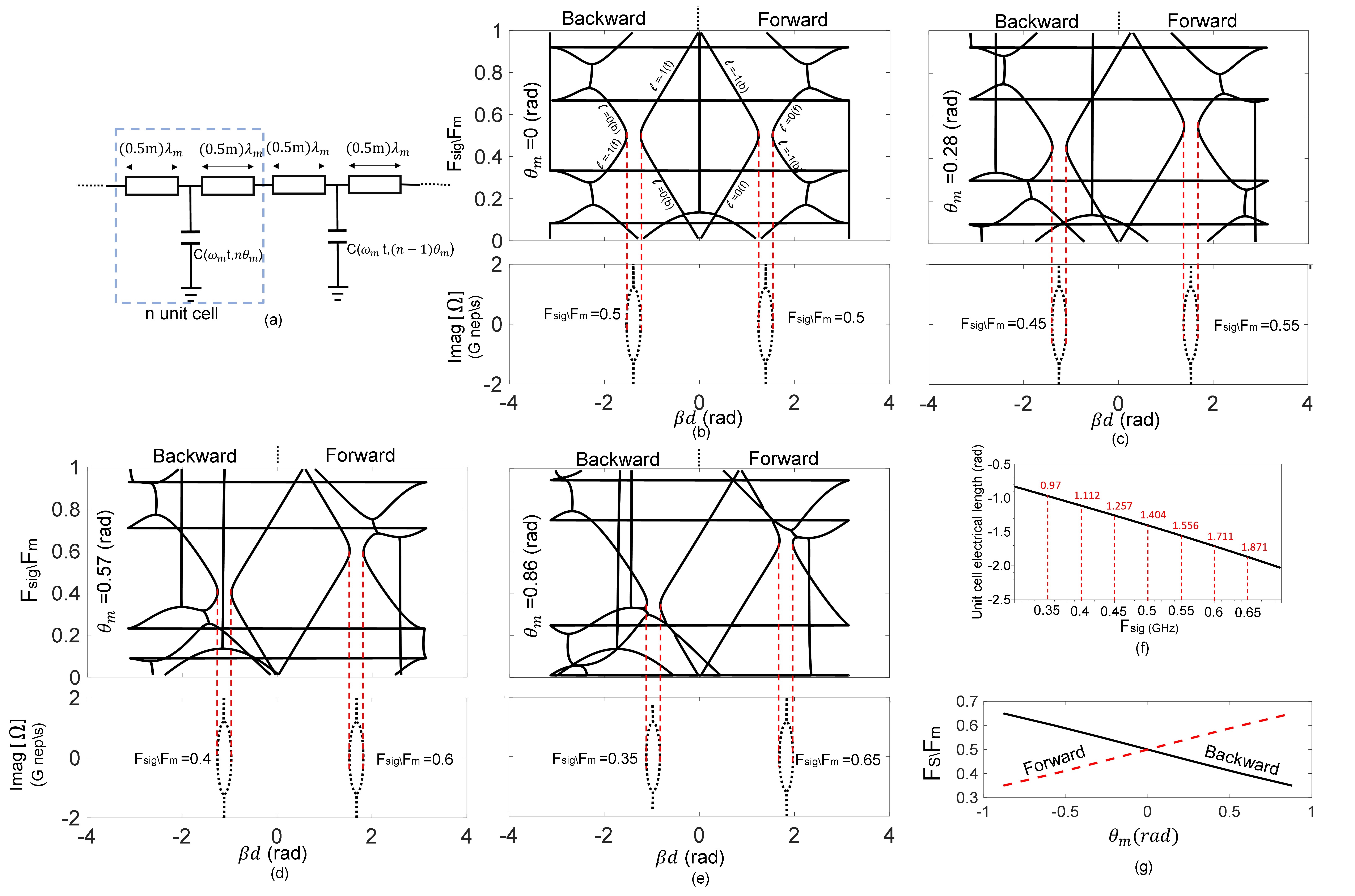
Figure 1: (a) T-shape unit cell with a time-invariant TL of length $0.5m~{}\lambda_{m}$ as series element and space-time modulated capacitor as shunt element. Real and complex frequency dispersion diagram with $N=2$ for the unit cell in (a) with $m=0.3$, $C_{o}=~{}4~{}$pF, $M_{D}=0.7$, $F_{m}=1$ GHz and TL $Z_{o}=$ $83~{}\Omega$ at (b) $\theta_{m}=~{}0$ rad, (c) $\theta_{m}=~{}0.28$ rad, (d) $\theta_{m}=~{}0.57$ rad and (e) $\theta_{m}=~{}0.86$ rad. (f) Unit cell electrical length variation with frequency at $C_{o}$. (g) Signal growth frequency variation for forward and backward propagation with $\theta_{m}$. (In Fig.1(b) $l$ is the order of harmonic with (f) and (b) referring to forward and backward propagation, respectively.)

Wave growth in nonreciprocal dispersion diagram of space-time modulated TL.$-$ For the unit cell shown in Fig. 1(a), the Bloch impedance ($Z_{Bloch}$) of the unit cell is chosen to be 50 $\Omega$ at $F_{sig}=0.5$ GHz. As result, $C_{o}$, TL characteristic impedance $Z_{o}$ and $m$ are set to $4$  pF, $83~{}\Omega$ and $0.3$, respectively. The dispersion diagram (DD) is plotted in Fig. 1(b) considering only time modulation ($F_{m}=1$ GHz and $\theta_{m}=~{}0$) and $M_{D}=0.7$ with $N=2$. At $F_{sig}=0.5$ GHz ($F_{m}=2F_{sig}$), a phase matching occurs between the fundamental $\omega_{sig}$ and the harmonic $\omega_{-1}$ in forward and backward propagations. The matching phase equals the unit cell electrical length at $C_{o}$ ($UCEL_{C_{o}}$). Consequently, strong interaction happens, and momentum band gaps (MBG) for forward and backward propagation are formed, in which no relation between real frequency and phase exists [10, 14]. As shown in Fig. 1(b), within the MBG, only complex frequency ($\omega_{sig}$ and $\omega_{-1}$) exists with a constant real part equal $F_{sig}=0.5$ GHz ($F_{m}=2F_{sig}$) and varying imaginary part. The imaginary part has positive values (causing wave growth) and negative values (causing wave decay) with a maximum centered at the middle of the gap. This behavior is similar to the exceptional point physics [25, 26]. The complex frequency dispersion relation is plotted using the following equation instead of (2)

$$\Omega=\omega_{l}-i\sigma_{l}$$ (18)

Next, in addition to time modulation, space modulation is considered by imposing a progressive phase shift ($-\theta_{m}$) to the modulation between successive cells. we will focus on the substantial harmonics $\omega_{0}$ and $\omega_{-1}$ that are linked to the MPGs. According to (12), the dispersion lines of fundamental $\omega_{sig}$ are not affected. On the other hand, the forward and backward dispersion lines of harmonic $\omega_{-1}$ are shifted in a way that causes the forward and backward MPGs to be settled at two different frequencies following

$${UCEL_{C_{o}}\ at\ \left(F_{f}\right)}-{UCEL_{C_{o}}\ at\ \left(F_{b}\right)}=\theta_{m}$$ (19)

where $F_{f}$ and $F_{b}$ are the frequencies at which MBGs are formed at forward and backward propagation, respectively. In addition, $F_{f}$ and $F_{b}$ are related as

$$\frac{F_{f}+F_{b}}{F_{m}}=1$$ (20)

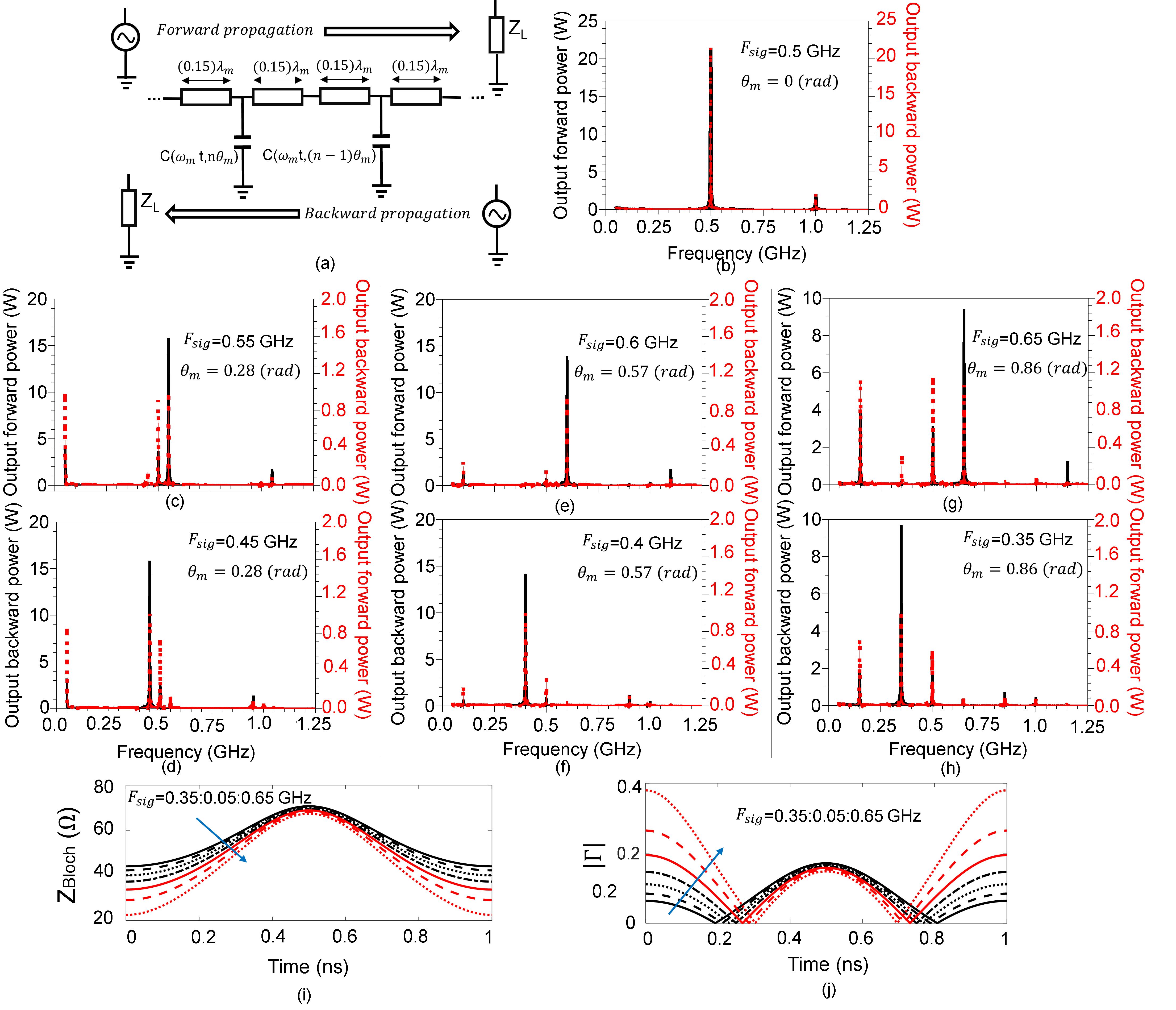
Figure 2: (a) Simulated nine unit cells with 1 W input power, TLs of length $0.15\lambda_{m}$, $Z_{o}=83~{}\Omega$, $C_{o}=4$ pF, $F_{m}=1$ GHz, $M_{D}=0.7$ loaded with a $50~{}\Omega$ load impedance. Forward (backward) propagation is defined in the direction where the phase shift between successive cells is $-\theta_{m}$ ($\theta_{m}$). Output forward and backward power in case (b) input frequency $F_{sig}=0.5$ GHz and $\theta_{m}=0$ rad, (c) $F_{sig}=0.55$ GHz and $\theta_{m}=0.28$ rad, (d) $F_{sig}=0.45$ GHz and $\theta_{m}=0.28$ rad, (e) $F_{sig}=0.6$ GHz and $\theta_{m}=0.57$ rad, (f) $F_{sig}=0.4$ GHz and $\theta_{m}=0.57$ rad, (g) $F_{sig}=0.65$ GHz and $\theta_{m}=0.86$ rad, (h) $F_{sig}=0.35$ GHz and $\theta_{m}=0.86$ rad. At different values of $F_{sig}$ and with time dependence, (i) unit cell $Z_{Bloch}$, (j) reflection coefficient considering $50~{}\Omega$ load and source.

Equation (19) describes the required value of $\theta_{m}$ that makes harmonics $\omega_{0}$ and $\omega_{-1}$ match phases at $C_{o}$ at specific frequencies. It works precisely to define wave growth frequencies at low values of $M_{D}$; however, as $M_{D}$ increases, required $\theta_{m}$ deviates slightly from (19) and can be easily optimized. This happens because the unit cell has time-invariant elements, TLs. As a result, the unit cell $Z_{Bloch}$ does not follow the capacitance variation in a linear behavior. Hence, considering only time modulation, harmonics $\omega_{0}$ and $\omega_{-1}$ matching phases at $C_{o}$ shift from the MPG center. When spatiotemporal modulating the line, wave growth frequencies shift slightly from the frequencies at which harmonics $\omega_{0}$ and $\omega_{-1}$ match phases at $C_{o}$, and a minor optimization is needed. For further investigation, DDs are plotted for $\frac{F_{f}}{F_{m}}$ values $0.55$, $0.6$ and $0.65$ in Figs. 1(c-e), respectively. As shown, $\frac{F_{b}}{F_{m}}$ exactly follows (20). On the other hand, the calculated electrical lengths of the unit cell at different frequencies, shown in Fig. 1(f), are utilized in (19) to obtain the initial value of $\theta_{m}$ and then optimized. At the exact value of $\theta_{m}$ associated with a desired $\frac{F_{f}}{F_{m}}$ ($\frac{F_{b}}{F_{m}}$), complex frequencies exist with a varying imaginary part and fixed real part defined by the desired $\frac{F_{f}}{F_{m}}$ ($\frac{F_{b}}{F_{m}}$). For $\frac{F_{f}}{F_{m}}$ ($\frac{F_{b}}{F_{m}}$) values $0.55$ ($0.45$), $0.6$ ($0.4$) and $0.65$ ($0.35$), $\theta_{m}$ optimized values are found to be $0.28$, $0.57$ and $0.86$ rad, respectively. Moreover, as shown in Figs. 1(b-e), imaginary part values of $\Omega$ are almost the same at different values of $\theta_{m}$. Consequently, the same wave growth rate is expected if the same boundary conditions exist. According to Fig. 1(g), $\frac{F_{f}}{F_{m}}$ and $\frac{F_{b}}{F_{m}}$ can take variety of values lower or higher than $0.5$ by choosing the proper value and sign of $\theta_{m}$, (20) is always applied.

Circuit Modeling.$-$ Scenarios presented in Figs.1(b-e) are verified using transient simulations (TS) and circuit modeling. As illustrated in Fig. 2(a), nine-unit cells are considered with 1 W input power source followed by $50~{}\Omega$ isolator and $50~{}\Omega$ load impedance. TLs have a length of $0.15\lambda_{m}$ and $Z_{o}=83~{}\Omega$. The capacitor has $C_{o}=4$ pF and time-modulated with $F_{m}=1$ GHz and $M_{D}=0.7$. Output forward (backward) power is the output power when the source and the load are connected to the terminals with a $-\theta_{m}$ ($\theta_{m}$) phase shift between successive cells, as shown in Fig. 2(a). In all considered cases, TS output results are Fourier transformed and plotted in Figs. 2(b-h).

For input frequency ($F_{sig}$) equals $0.5$ GHz and $\theta_{m}=0$ rad, as shown in Fig. 2(b), the output forward power (OFP) and output backward power (OBP) are identical with a gain more than $13$ dB, congruent with Figs. 1(b). Moreover, following Figs. 1(c) and considering $F_{sig}=0.55$ ($0.45$) GHz with $\theta_{m}=0.28$ rad, OFP (OBP) is amplified to $11.7$ dB while no gain is achieved in OBP (OFP) as illustrated in Figs. 2(c-d). Finally, by following Figs. 1(d)/(e) and considering $F_{sig}=0.6$/$0.65$ ($0.4$/$0.35$) GHz with $\theta_{m}=0.57$/$0.86$ rad, OFP (OBP) is amplified to $11.4$/$10$ dB without any gain in OBP (OFP) as shown in Figs. 2(e-f)/(g-h).

As illustrated in Figs. 1(b-e), when space-time modulating the TL, it is expected to have the same growth rate if the boundary conditions are the same. In the simulations illustrated in Fig. 2, loaded TL is terminated in all cases with a fixed $50~{}\Omega$ impedance at the source and the load. The TL is matched at $C_{o}$ and $F_{sig}=0.5$ GHz to a fixed $50~{}\Omega$ impedance. However, shifting from $F_{sig}=0.5$ GHz changes the $Z_{Bloch}$ profile, Fig. 2(i), with modulation period (T_m) which changes the reflection coefficient profile at the terminals, Figs. 2(j). Consequently, the boundary conditions change, resulting in a growth rate variation shown in Fig. 2. However, studying the detailed effect of boundary conditions variation on amplification gain is beyond the scope of this letter.

In conclusion, reconfigurable nonreciprocal wave growth in a space-time modulated TL is confirmed through eigenvalue problem solution and circuit modeling. TL is time-modulated by loading sinusoidally time-modulated capacitors and space-modulated by forcing a modulation phase shift $-\theta_{m}$ between successive cells. Varying $\theta_{m}$ causes MPGs to shift from $F_{signal}=0.5~{}F_{modulation}$ in a nonreciprocal behavior. As a result, nonreciprocal wave growth frequencies are obtained.

This work has been completed under a research agreement between Purdue University and The American University in Cairo.

References

- Sturrock [1958] P. A. Sturrock, Kinematics of growing waves, Phys. Rev. 112, 1488 (1958).
- Fainberg [1962] Y. B. Fainberg, Interaction of charged-particle beams with plasma, The Soviet Journal of Atomic Energy 11, 958 (1962).
- Briggs [1964] R. J. Briggs, Electron-Stream Interaction with Plasmas (The MIT Press, 1964).
- CULLEN [1958] A. L. CULLEN, A travelling-wave parametric amplifier, Nature 181, 332 (1958).
- Tien [1958] P. K. Tien, Parametric amplification and frequency mixing in propagating circuits, Journal of Applied Physics 29, 1347 (1958).
- Huang [2018] J. Huang, Parametric amplifiers in optical communication systems: From fundamentals to applications, in Optical Amplifiers - A Few Different Dimensions (InTech, 2018).
- Yu and Fan [2009] Z. Yu and S. Fan, Erratum: Complete optical isolation created by indirect interband photonic transitions, Nature Photonics 3, 303 (2009).
- Ruesink et al. [2016] F. Ruesink, M.-A. Miri, A. Alù, and E. Verhagen, Nonreciprocity and magnetic-free isolation based on optomechanical interactions, Nature Communications 7, 10.1038/ncomms13662 (2016).
- Li et al. [2021] H. Li, S. Yin, E. Galiffi, and A. Alù, Temporal parity-time symmetry for extreme energy transformations, Phys. Rev. Lett. 127, 153903 (2021).
- Lustig et al. [2018] E. Lustig, Y. Sharabi, and M. Segev, Topological aspects of photonic time crystals, Optica 5, 1390 (2018).
- Wang et al. [2021] K. Wang, A. Dutt, C. C. Wojcik, and S. Fan, Topological complex-energy braiding of non-hermitian bands, Nature 598, 59 (2021).
- Joannopoulos et al. [2008] J. D. Joannopoulos, S. G. Johnson, J. N. Winn, and R. D. Meade, Photonic crystals, 2nd ed. (Princeton University Press, Princeton, NJ, 2008).
- Sievenpiper et al. [1999] D. F. Sievenpiper, L. Zhang, R. J. Broas, N. g. Alexopolous, and E. Yablonovitch, High-impedance electromagnetic surfaces with a forbidden frequency band, IEEE Transactions on Microwave Theory and Techniques 47, 2059 (1999).
- Galiffi et al. [2022] E. Galiffi, R. Tirole, S. Yin, H. Li, S. Vezzoli, P. A. Huidobro, M. G. Silveirinha, R. Sapienza, A. Alù, and J. B. Pendry, Photonics of time-varying media, Advanced Photonics 4, 014002 (2022).
- Galiffi et al. [2023] E. Galiffi, G. Xu, S. Yin, H. Moussa, Y. Ra’di, and A. Alù, Broadband coherent wave control through photonic collisions at time interfaces, Nature Physics 10.1038/s41567-023-02165-6 (2023).
- Wang et al. [2023] X. Wang, M. S. Mirmoosa, V. S. Asadchy, C. Rockstuhl, S. Fan, and S. A. Tretyakov, Metasurface-based realization of photonic time crystals, Science Advances 9, eadg7541 (2023).
- Sounas and Alù [2017] D. L. Sounas and A. Alù, Non-reciprocal photonics based on time modulation, Nature Photonics 11, 774 (2017).
- Bhandare et al. [2005] S. Bhandare, S. Ibrahim, D. Sandel, H. Zhang, F. Wust, and R. Noe, Novel nonmagnetic 30-db traveling-wave single-sideband optical isolator integrated in iii/v material, IEEE Journal of Selected Topics in Quantum Electronics 11, 417 (2005).
- Hadad et al. [2015] Y. Hadad, D. L. Sounas, and A. Alu, Space-time gradient metasurfaces, Physical Review B 92, 10.1103/physrevb.92.100304 (2015).
- Qin et al. [2014] S. Qin, Q. Xu, and Y. E. Wang, Nonreciprocal components with distributedly modulated capacitors, IEEE Transactions on Microwave Theory and Techniques 62, 2260 (2014).
- He et al. [2023] H. He, S. Zhang, J. Qi, F. Bo, and H. Li, Faraday rotation in nonreciprocal photonic time-crystals, Applied Physics Letters 122, 10.1063/5.0131818 (2023).
- Elnaggar and Milford [2020] S. Y. Elnaggar and G. N. Milford, Modeling space–time periodic structures with arbitrary unit cells using time periodic circuit theory, IEEE Transactions on Antennas and Propagation 68, 6636 (2020).
- Jayathurathnage et al. [2021] P. Jayathurathnage, F. Liu, M. S. Mirmoosa, X. Wang, R. Fleury, and S. A. Tretyakov, Time-varying components for enhancing wireless transfer of power and information, Physical Review Applied 16, 10.1103/physrevapplied.16.014017 (2021).
- Elnaggar and Milford [2021] S. Y. Elnaggar and G. N. Milford, Properties of translation operator and the solution of the eigenvalue and boundary value problems of arbitrary space–time periodic metamaterials, Royal Society Open Science 8, 210367 (2021).
- Bergholtz et al. [2021] E. J. Bergholtz, J. C. Budich, and F. K. Kunst, Exceptional topology of non-hermitian systems, Rev. Mod. Phys. 93, 015005 (2021).
- Miri and Alù [2019] M.-A. Miri and A. Alù, Exceptional points in optics and photonics, Science 363, 10.1126/science.aar7709 (2019).