Constructing disjoint Steiner trees in Sierpiński graphs

Abstract

Let $G$ be a graph and $S\subseteq V(G)$ with $|S|\geq 2$. Then the trees $T_{1},T_{2},\cdots,T_{\ell}$ in $G$ are internally disjoint Steiner trees connecting $S$ (or $S$-Steiner trees) if $E(T_{i})\cap E(T_{j})=\emptyset$ and $V(T_{i})\cap V(T_{j})=S$ for every pair of distinct integers $i,j$, $1\leq i,j\leq\ell$. Similarly, if we only have the condition $E(T_{i})\cap E(T_{j})=\emptyset$ but without the condition $V(T_{i})\cap V(T_{j})=S$, then they are edge-disjoint Steiner trees. The generalized $k$-connectivity, denoted by $\kappa_{k}(G)$, of a graph $G$, is defined as $\kappa_{k}(G)=\min\{\kappa_{G}(S)|S\subseteq V(G)\ \textrm{and}\ |S|=k\}$, where $\kappa_{G}(S)$ is the maximum number of internally disjoint $S$-Steiner trees. The generalized local edge-connectivity $\lambda_{G}(S)$ is the maximum number of edge-disjoint Steiner trees connecting $S$ in $G$. The generalized $k$-edge-connectivity $\lambda_{k}(G)$ of $G$ is defined as $\lambda_{k}(G)=\min\{\lambda_{G}(S)\,|\,S\subseteq V(G)\ and\ |S|=k\}$. These measures are generalizations of the concepts of connectivity and edge-connectivity, and they and can be used as measures of vulnerability of networks. It is, in general, difficult to compute these generalized connectivities. However, there are precise results for some special classes of graphs. In this paper, we obtain the exact value of $\lambda_{k}(S(n,\ell))$ for $3\leq k\leq\ell^{n}$, and the exact value of $\kappa_{k}(S(n,\ell))$ for $3\leq k\leq\ell$, where $S(n,\ell)$ is the Sierpiński graphs with order $\ell^{n}$. As a direct consequence, these graphs provide additional interesting examples when $\lambda_{k}(S(n,\ell))=\kappa_{k}(S(n,\ell))$. We also study the some network properties of Sierpiński graphs.
Keywords: Steiner Tree; Generalized Connectivity; Sierpiński Graph.
AMS subject classification 2010: 05C40, 05C85.

1 Introduction

All graphs considered in this paper are undirected, finite and simple. We refer the readers to [1] for graph theoretical notation and terminology not described here. For a graph $G$, let $V(G)$ and $E(G)$ denote the set of vertices and the set of edges of $G$, respectively. The neighborhood set of a vertex $v\in V(G)$ is $N_{G}(v)=\{u\in V(G)\,|\,uv\in E(G)\}$. The degree of a vertex $v$ in $G$ is denoted by $d(v)=|N_{G}(v)|$. Denote by $\delta(G)$ ($\Delta(G)$) the minimum degree (maximum degree) of the graph $G$. For a vertex subset $S\subseteq V(G)$, the subgraph induced by $S$ in $G$ is denoted by $G[S]$ and similarly $G[V\setminus S]$ for $G\setminus S$ or $G-S$. Especially, $G-v$ is $G[V\setminus\{v\}]$. Let $\overline{G}$ be the complement of $G$.

1.1 Generalized (edge-)connectivity

Connectivity and edge-connectivity are two of the most basic concepts of graph-theoretic measures. Such concepts can be generalized, see, for example, [16]. For a graph $G=(V,E)$ and a set $S\subseteq V(G)$ of at least two vertices, an $S$-Steiner tree or a Steiner tree connecting $S$ (or simply, an $S$-tree) is a subgraph $T=(V^{\prime},E^{\prime})$ of $G$ that is a tree with $S\subseteq V^{\prime}$. Note that when $|S|=2$ a minimal $S$-Steiner tree is just a path connecting the two vertices of $S$.

Let $G$ be a graph and $S\subseteq V(G)$ with $|S|\geq 2$. Then the trees $T_{1},T_{2},\cdots,T_{\ell}$ in $G$ are internally disjoint $S$-trees if $E(T_{i})\cap E(T_{j})=\emptyset$ and $V(T_{i})\cap V(T_{j})=S$ for every pair of distinct integers $i,j$, $1\leq i,j\leq\ell$. Similarly, if we only have the condition $E(T_{i})\cap E(T_{j})=\emptyset$ but without the condition $V(T_{i})\cap V(T_{j})=S$, then they are edge-disjoint $S$-trees (Note that while we do not have the condition $V(T_{i})\cap V(T_{j})=S$, it is still true that $S\subseteq V(T_{i})\cap V(T_{j})$ as $T_{i}$ and $T_{j}$ are $S$-trees.) The generalized $k$-connectivity, denoted by $\kappa_{k}(G)$, of a graph $G$, is defined as $\kappa_{k}(G)=\min\{\kappa_{G}(S)|S\subseteq V(G)\ \textrm{and}\ |S|=k\}$, where $\kappa_{G}(S)$ is the maximum number of internally disjoint $S$-trees. The generalized local edge-connectivity $\lambda_{G}(S)$ is the maximum number of edge-disjoint $S$-trees in $G$. The generalized $k$-edge-connectivity $\lambda_{k}(G)$ of $G$ is defined as $\lambda_{k}(G)=\min\{\lambda_{G}(S)\,|\,S\subseteq V(G)\ and\ |S|=k\}$. Since internally disjoint S-trees are edge-disjoint but not vice versa, it follows from the definitions that $\kappa_{k}(G)\leq\lambda_{k}(G)$.

It is well-known that the classical edge-connectivity has two equivalent definitions. The edge-connectivity of $G$, written $\lambda(G)$, is the minimum size of an edge-subset $M\subseteq E(G)$ such that $G\setminus M$ is disconnected. The local edge-connectivity $\lambda_{G}(x,y)$ is defined as the maximum number of edge-disjoint paths between $x$ and $y$ in $G$ for a pair of distinct vertices $x$ and $y$ of $G$. For the graph $G$ we can get a global quantity $\lambda^{*}(G)=\min\{\lambda_{G}(x,y)\,|\,x,y\in V(G),\,x\neq y\}$. The edge version of Menger’s theorem says that $\lambda(G)$ is equal to $\lambda^{*}(G)$. This result can be found in [1]. It is clear that when $|S|=2$, $\lambda_{2}(G)$ is just the standard edge-connectivity $\lambda(G)$ of $G$, that is, $\lambda_{2}(G)=\lambda(G)$, and $\kappa_{2}(G)=\kappa(G)$, that is, the standard connectivity of $G$. Thus $\kappa_{k}(G)$ and $\lambda_{k}(G)$ are the generalized connectivity of $G$ and the generalized edge-connectivity of $G$, respectively. Moreover, we set $\lambda_{k}(G)=\kappa_{k}(G)=0$ when $G$ is disconnected. As remarked earlier, $\kappa_{k}(G)\leq\lambda_{k}(G)$. The standard example showing that $\kappa(G)$ can be much smaller than $\lambda(G)$ can be modified to show that $\kappa_{k}(G)$ can be much smaller than $\lambda_{k}(G)$. We can take $k$ copies of $K_{n}$ and pick one vertex from each copy to identify into one vertex $v$. Then if we pick one vertex from each copy other than $v$ to form $S$, $\kappa_{G}(S)=1$, and hence $\kappa_{k}(G)=1$. One can use Theorem 1.1 from the next section to see that $\lambda_{k}(G)$ is much larger. There are many results on generalized (edge-)connectivity; see the book [15] by Li and Mao.

Problem 1.

Find more examples of graphs $H$ such that $\lambda_{k}(H)=\kappa_{k}(H)$.

There are many results of generalized connectivity of special networks/graphs, and most of them are restricted to $k=3$ or $4$. Li et al. [14] gave the exact value of generalized $3$-connectivity of star graphs and bubble-sort graphs. Zhao and Hao [27] investigated the generalized $3$-connectivity of alternating group graphs and $(n,k)$-star graphs. We list some known results on the generalized connectivity of some known networks and special graphs; see Table 1.

Table 1: Generalized connectivity of some known networks

Graphs or networks	Generalized $k$-connectivity				Reference
	$k=3$	$k=4$	$k$	$k=n$
Sierpiński graphs $S(n,\ell)$	$\ell-1$	$\ell-2$	$\ell-\lceil k/2\rceil$	$\lceil\ell/2\rceil$	*
Complete graph $K_{n}$	$n-1$	$n-2$	$n-\lceil k/2\rceil$	$\lceil n/2\rceil$	[4]
Data center network $D_{\ell,n}$	$n+\ell-2$	*	*	*	[9]
Bubble-sort graph $B_{n,\ell}$	$n-2$	*	*	*	[25]
($n,k$)-star graph $S_{n,\ell}$	$n-2$	$n-2$	*	*	[29, 18]
Alternating group graph $AG_{n}$	$2n-5$	*	*	*	[29]
Hypercube $Q_{n}$	$n-1$	$n-1$	*	*	[19, 20]
Alternating group graph $AG_{n}$	$2n-5$	*	*	*	[29]
Pancake graph $PA_{n}$	*	$n-2$	*	*	[32]
Hierarchical cubic network $HCN_{n}$	$n$	$n$	*	*	[31]
Exchanged hypercube $EH(s,t))$	$\min\{s,t\}$	$\min\{s,t\}$	*	*	[30]

For other results, we refer the readers to [26, 28, 17, 12, 13].

As it is well-known, for any graph $G$, we have polynomial-time algorithms to find the classical connectivity $\kappa(G)$ and edge-connectivity $\lambda(G)$. Given two fixed positive integers $k$ and $\ell$, for any graph $G$ the problem of deciding whether $\lambda_{k}(G)\geq\ell$ can be solved by a polynomial-time algorithm. If $k\ (k\geq 3)$ is a fixed integer and $\ell\ (\ell\geq 2)$ is an arbitrary positive integer, the problem of deciding whether $\kappa(S)\geq\ell$ is $NP$-complete. For any fixed integer $\ell\geq 3$, given a graph $G$ and a subset $S$ of $V(G)$, deciding whether there are $\ell$ internally disjoint Steiner trees connecting $S$, namely deciding whether $\kappa(S)\geq\ell$, is $NP$-complete. For more details on the computational complexity of generalized connectivity and generalized edge-connectivity, we refer to the book [15].

In addition to being a natural combinatorial measure, generalized $k$-connectivity can be motivated by its interesting interpretation in practice. For example, suppose that $G$ represents a network. If one wants to “connect” a pair of vertices of $G$ “minimally,” then a path is used to “connect” them. More generally, if one wants to “connect” a set $S$ of vertices of $G$, with $|S|\geq 3$, “minimally,” then it is desirable to use a tree to “connect” them. Such trees are precisely $S$-trees, which are also used in computer communication networks (see [8]) and optical wireless communication networks (see [6]).

From a theoretical perspective, generalized edge-connectivity is related to Nash-Williams-Tutte theorem and Menger theorem; see [15]. The generalized edge-connectivity has applications in $VLSI$ circuit design. In this application, a Steiner tree is needed to share an electronic signal by a set of terminal nodes. Another application, which is our primary focus, arises in the Internet Domain. Imagine that a given graph $G$ represents a network. We arbitrarily choose $k$ vertices as nodes. Suppose one of the nodes in $G$ is a broadcaster, and all other nodes are either users or routers (also called switches). The broadcaster wants to broadcast as many streams of movies as possible, so that the users have the maximum number of choices. Each stream of movie is broadcasted via a tree connecting all the users and the broadcaster. So, in essence we need to find the maximum number Steiner trees connecting all the users and the broadcaster, namely, we want to get $\lambda(S)$, where $S$ is the set of the $k$ nodes. Clearly, it is a Steiner tree packing problem. Furthermore, if we want to know whether for any $k$ nodes the network $G$ has above properties, then we need to compute $\lambda_{k}(G)=\min\{\lambda(S)\}$ in order to prescribe the reliability and the security of the network. For more details, we refer to the book [15].

By the definition of the generalized $k$-connectivity, the following observation is immediate.

Observation 1.

Let $n,k$ be two integers with $2\leq k\leq n$. If $H$ is a spanning subgraph of $G$, then $\kappa_{k}(H)\leq\kappa_{k}(G)$.

Chartrand et al. [4] and Li et al. [16] obtained the exact value of $\kappa_{k}(K_{n})$.

Theorem 1.1 ([16, 4]).

For every two integers $n$ and $k$ with $2\leq k\leq n$,

$$\kappa_{k}(K_{n})=\lambda_{k}(K_{n})=n-\lceil k/2\rceil.$$

Lemma 1.1.

[15] For two integers $k$ and $n$ with $2\leq k\leq n-1$ and a connected graph $G$, we have

$$\lambda_{k+1}(G)\leq\lambda_{k}(G).$$

Moreover, the upper bound is sharp.

1.2 Sierpiński graphs

In 1997, Sandi Klav̆ar and Uros̆ Milutinović introduced the concept of Sierpiński graph $S(n,\ell)$ in [11]. We denote $n$-tuples $V^{n}$ by the set

$$V^{n}=\{\langle u_{0}u_{1}\cdots u_{n-1}\rangle|\ u_{i}\in\{0,1,\ldots,\ell-1\}\textrm{ and }i\in\{0,1,\ldots,n-1\}\}.$$

A word $u$ of size $n$ are denoted by $\langle u_{0}u_{1},\cdots,u_{n-1}\rangle$ in which $u_{i}\in\{0,\ldots,\ell-1\}$. The concatenation of two words $u=\langle u_{0}u_{1}\cdots u_{n-1}\rangle$ and $v=\langle v_{0}v_{1}\cdots v_{n-1}\rangle$ is denoted by $uv$.

Definition 1.

The Sierpiński graph $S(n,\ell)$ is defined as below, for $n\geq 1$ and $\ell\geq 3$, the vertex set of $S(n,\ell)$ consists of all $n$-tuples of integers $0,1,\cdots,\ell-1$. That is $V(S(n,\ell))=V^{n}$, where $uv=(u_{0}u_{1}\cdots u_{n-1},v_{0}v_{1}\cdots v_{n-1})$ is an edge of $E(S(n,\ell))$ if and only if there exists $d\in\{0,1,\ldots,\ell-1\}$ such that: $(1)$ $u_{j}=v_{j}$, if $j<d$; $(2)$ $u_{d}\neq v_{d}$; $(3)$ $u_{j}=v_{d}$ and $v_{j}=u_{d}$, if $j>d$.

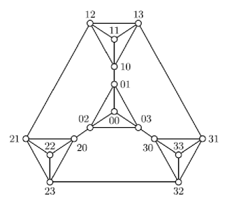
Figure 1: $S(2,4)$

Sierpiński graph $S(2,4)$ is show in figure 1. Note that $S(n,\ell)$ can be constructed recursively as follows: $S(1,\ell)$ is isomorphic to $K_{\ell}$, which vertex set is 1-tuples set $\{0,\cdots,\ell\}$. To construct $S(n,\ell)$ for $n>1$, take copies of $\ell$ times $S(n-1,\ell)$ and add to labels of vertices in copy $i$ of $S(n-1,\ell)$ the letter $i$ at the beginning. Note that there is exactly one edge (bridge edge) between $S^{i}(n,\ell)$ and $S^{j}(n,\ell)$, $i\neq j$, namely the edge between vertices $\langle ij\cdots j\rangle$ and $\langle ji\cdots i\rangle$.

The vertices $(\underbrace{i,i,\cdots,i}_{n})$, $i\in\{0,1,\ldots,\ell-1\}$ are the extreme vertices of $S(n,\ell)$. Note that an extreme vertex $u$ of $S(n,\ell)$ has degree $d(u)=\ell-1$. For $i\in\{0,\ldots,\ell-1\}$ and $n\geq 2$, let $S^{i}(n-1,\ell)$ denote the subgraph of $S(n,\ell)$ induced by the vertices of the form $\{\langle i\underbrace{u_{1}\cdots u_{n-1}}_{n-1}\rangle\,|\,0\leq u_{i}\leq\ell-1\}$. Furthermore, for $t_{n-s}=\underbrace{u_{1}\cdots u_{n-s}}_{n-s}$, it is obvious that $S^{t_{n-s}}(s,\ell)$ is subgraph induced by the prefix $\langle\underbrace{u_{1},\cdots,u_{n-s}}_{n-s}\cdots\rangle$ in $V(S(n,\ell))$.

Sierpínski graphs generalize Hanoi graphs which can be viewed as “discrete” finite versions of a Sierpinski gasket [22, 10]. Xue considered the Hamiltionicity and path $t$-coloring of Sierpínski-like graphs in [23]; furthermore, they proved that $Val(S(n,k))=Val(S[n,k])=\lfloor k/2\rfloor$, where $Val(S(n,k))$ is the linear arboricity of Sierpínski graphs. We remark that although Sierpínski graphs are not regular, they are “almost” regular as the extreme vertices have degrees one less than the degrees of non-extreme vertices. The following result is on the Hamiltonian decomposition of Sierpínski graphs.

Theorem 1.2.

[23] $(1)$ For even $\ell\geq 2$, $S(n,\ell)$ can be decomposed into edge disjoint union of $\frac{\ell}{2}$ Hamiltonian paths of which the end vertices are extreme vertices.

$(2)$ For odd $\ell\geq 3$, there exists $\frac{\ell-1}{2}$ edge disjoint Hamiltonian paths whose two end vertices are extreme vertices in $S(n,\ell)$.

In fact, Theorem 1.2 is used in the proof of Theorem 1.3, which give an lower bound for the generalized $k$-edge connectivity of Sierpínski graphs $S(n,\ell)$.

1.3 Our results

The following two observations are immediate.

Observation 2.

For $S(n,\ell)$, recall that the vertex set $V(S(n,\ell))$ can be partitioned into $\ell$ parts, say $V(S^{0}(n-1,\ell)),V(S^{1}(n-1,\ell)),\ldots,V(S^{\ell-1}(n-1,\ell))$, where $V(S^{i}(n-1,\ell))$ is an induced subgraph on vertex set $\{(iu_{1}\cdots u_{n-1})\,|\,u_{1}\cdots u_{n-1}$ ranges over all of $\{0,1,\ldots,\ell-1\}^{n-1}\}$.

$(1)$ for each $0\leq i\leq\ell-1$, $S^{i}(n-1,\ell)$ is isomorphic to $S(n-1,\ell)$.

$(2)$ $S(n,\ell)=S^{0}(n-1,\ell)\oplus\cdots\oplus S^{\ell-1}(n-1,\ell)$, where $\oplus$ means that $V(S(n,\ell))=V(S^{0}(n-1,\ell))\cup\cdots\cup V(S^{\ell-1}(n-1,\ell))$ and $S(n,\ell)$ is the graph obtained from $S^{0}(n-1,\ell),\cdots,S^{\ell-1}(n-1,\ell)$ by adding exactly one edge (bridge edge) between $S^{i}(n-1,\ell)$ and $S^{j}(n-1,\ell)$, $i\neq j$, where the vertices set of bridge edge is $\{\langle ij\cdots j\rangle,\langle ji\cdots i\rangle\}$.

Consider the Sierpiński graph $S(n,\ell)$, for vertex $u=iu_{1}\cdots u_{n-1}$ of $S^{i}(n-1,\ell)$, the unique neighbor of $u$ outside of $S^{i}(n-1,\ell)$ (call it the out-neighbor of $u$) is written as $u^{\prime}$. We call the neighbors of $u$ in $S^{i}(n-1,\ell)$ the in-neighbors of $u$.

Observation 3.

$(1)$ For two distinct vertices of $S^{i}(n-1,\ell)$ for $0\leq i\leq\ell$, if they have out-neighbors, then the out-neighbors are in different .

$(2)$ The $S^{i}(n-1,\ell)$ and $S^{j}(n-1,\ell)$ are connected by a single bridge edges between vertex $(i\underbrace{jj\cdots j}_{n-1})$ and $(j\underbrace{ii\cdots i}_{n-1})$.

Motivated by giving exact values of generalized connectivity for general $k$ and Problem 1, we derive the following result.

Theorem 1.3.

$(i)$ For $3\leq k\leq\ell$, we have

$$\kappa_{k}(S(n,\ell))=\lambda_{k}(S(n,\ell))=\ell-\left\lceil k/2\right\rceil.$$

$(ii)$ For $\ell+1\leq k\leq{\ell}^{n}$, we have

$$\kappa_{k}(S(n,\ell))\leq\left\lfloor\ell/2\right\rfloor\mbox{ and }\lambda_{k}(S(n,\ell))=\left\lfloor\ell/2\right\rfloor.$$

2 Proof of Theorem 1.3

We prove Theorem 1.3 in this section. To accomplish this, we require the following existing result. Technically, we will be using its corollary.

Theorem 2.1 ([5, 24]).

Suppose $G$ is the complete graph with $V(G)=\{v_{0},\cdots,v_{N-1}\}$. If $N=2n$, then $G$ can be decomposed into $n$ Hamiltonian paths

$$\{i\in\{1,2,\ldots,n\}:\ L_{i}=v_{0+i}v_{1+i}v_{2n-1+i}v_{2+i}v_{2n-2+i}\cdots v_{n+1+i}v_{n+1}\},$$

the subscripts take modulo $2n$. If $N=2n+1$, then $G$ can be decomposed into $n$ Hamiltonian paths

$$\{i\in\{1,2,\ldots,n\}:\ L_{i}=\ v_{0+i}v_{1+i}v_{2n+i}v_{2+i}v_{2n-1+i}\cdots v_{n+i}v_{n+1+i}\}$$

and a matching $M=\{v_{n-i}v_{n+1}:\ i\in\{1,2,\ldots,n\}\}$, the subscripts take modulo $2n+1$.

Corollary 2.2.

Suppose $G$ is the complete graph with $V(G)=\{v_{1},\cdots,v_{N}\}$, $s\leq\frac{N}{2}$ and $\mathcal{S}=\{\ S_{i}=\{v_{i_{1}},v_{i_{2}}\}:i\in\{1,2,\ldots,s\}\}$ is a collection of pairwise disjoint $2$-subsets of $V(G)$. Then there are $s$ edge-disjoint Hamiltonian paths $L_{1},\cdots,L_{s}$ such that $v_{i_{1}},v_{i_{2}}$ are endpoints of $L_{i}$.

For $1\leq s<n$, by the definition of the Sierpiński graph $S(n,\ell)$, $G=S(n,\ell)$ consists of $\ell^{n-s}$ Sierpiński graphs $S(s,\ell)$, and we call each such $S(s,\ell)$ an $s$-atom of $G$. Note that $\mathcal{P}=\{V(H):\ H\mbox{ is an }s\mbox{-atom of }G\}$ is a partition of $V(G)$. We use $G_{s}$ to denote the graph $G/\mathcal{P}$. It is obvious that $G_{s}$ is a simple graph and $G_{s}=S(n-s,\ell)$. Note that $G_{n}$ is a single vertex and $G_{0}=G$. For a vertex $u$ of $G_{s}$, we use $A_{s,u}$ to denote the $s$-atom of $G$ which is contracted into $u$. See Figures 4, 4 and 4 for illustrations. In addition, we can also denote $A_{s,u}$ by $A_{u}$ if $u\in V(G_{s})$ is clear.

Note that $G_{s-1}$ is the graph obtained from $G_{s}$ by replacing each vertex $u$ with a complete graph $K_{\ell}$. We denote by $H^{u}$ the complete graph replacing $u$ (see Figures 4 and 4 for illustrations). For an edge $e=uv$ of $G_{s}$, $e$ is also an edge of $G_{s-1}$. We use $u_{e}$ and $v_{e}$ to denote the ends of $e$ in $G_{s-1}$, respectively, such that $u_{e}\in V(H^{u})$ and $v_{e}\in V(H^{v})$. (See Figure 5 for an illustration.)

Suppose that $U$ is a subset of $V(G)$ with $|U|=k$ and $3\leq k\leq l$. For the graph $G_{s}$, a vertex $u$ of $G_{s}$ is labeled if $V(A_{s,u})\cap U\neq\emptyset$, and $u$ is unlabeled otherwise. We use $U^{s}$ to denote the set of labeled vertices of $G_{s}$. For a labeled vertex $u$ of $G_{s}$, let $W^{u}=V(H^{u})\cap U^{s-1}$, that is, the set of labeled vertices in $H^{u}$. See Figure 4 as an example, if $U=\{u_{000},u_{001},u_{013},u_{122}\}$, then $U^{1}=\{u_{00},u_{01},u_{12}\}$ and $W^{u_{0}}=\{u_{00},u_{01}\}$ in Figure 4.

Figure 2: $G=G_{0}=S(3,4)$

Figure 3: The graph $G_{1}$

Figure 4: The graph $G_{2}$

For the Sierpiński graph $S(n,\ell)$, we have the following result.

Theorem 2.3.

Suppose $G=S(n,\ell)$ and $U$ is a subset of $V(G)$ with $|U|=k$, where $3\leq k\leq\ell$. Then $G$ has $c=\ell-\left\lceil k/2\right\rceil$ $U$-Steiner trees.

Suppose that $s^{\prime}$ is the minimum integer such that $G_{s^{\prime}}$ has exactly one labeled vertex. Let $v$ be the labeled vertex in $G_{s^{\prime}}$. Note that $s^{\prime}$ exists since $G_{n}$ consists of a single labeled vertex. Then $U\subseteq A_{s^{\prime},v}$. Thus, in order to find $c$ $U$-Steiner trees of $G$, we only need to find $c$ $U$-Steiner trees of $A_{s^{\prime},v}$. Hence, without loss of generality, we may assume that $G$ is a graph with $|U^{n-1}|\geq 2$. Therefore, $|U^{i}|\geq 2$ for $i\leq n-1$.

We construct a branching $\overrightarrow{T}$ with vertex set $V(\overrightarrow{T})=\bigcup_{i\in\{0,\ldots,n\}}\{x:\ x\in V(G_{i})\}$ and arc set $A(\overrightarrow{T})=\{(x,y):\ y\in H^{x}\}$. The root of $\overrightarrow{T}$ is denoted by $v_{root}$. For two different vertices $x,y$ of $V(\overrightarrow{T})$, if there is a direct path from $x$ to $y$, then we say that $x\prec y$ (or $y\succ x$). The following result is obviously.

Fact 1.

If $x_{i}\in V(\overrightarrow{T})$ for $i\in[p]$ and $x_{1}\prec x_{2}\prec\ldots\prec x_{p}$, then $\sum_{i\in[p]}|W^{x_{i}}|\leq k+p-1$.

Figure 5: From graph $G_{1}$ to $G_{2}$ by $u_{e}v_{e}$ contraction edge $uv$.

In order to prove Theorem 2.3, we only need to prove the following stronger result. The proof of Lemma 2.1 is technical and is via induction. Note that since $G_{n}$ is a single vertex and $G=G_{0}$, the induction is from $G_{n-1}$ to $G_{1}$. The basic idea is to use the Steiner trees of $G_{s}$ to construct appropriate Steiner trees of $G_{s-1}$. Since each vertex in $G_{s}$ corresponds to a complete graph in $G_{s-1}$, it is not a straightforward process to extend Steiner trees of $G_{s}$ to Steiner trees of $G_{s-1}$.

Lemma 2.1.

For $0\leq s\leq n$, $G_{s}$ has $c$ $U^{s}$-Steiner trees $T_{1},\cdots,T_{c}$ such that the following statement holds.

1. For each $u\in U^{s}$ (say $u\in W^{v}$ and hence $v$ is a labeled vertex of $G_{s+1}$ if $s\neq n$) and $i\in\{1,\ldots,c\}$, $d_{T_{i}}(u)\leq 2$.

Proof.

If $s=n$, then each $T_{i}$ is the empty graph and the result holds. Thus, suppose $s\leq n-1$. Hence, $v$ always exists. The following implies that the result holds for $s=n-1$. Note that $U^{n-1}=W^{v_{root}}$.

Claim 1.

If $s=n-1$, then we can construct $T_{1},\ldots,T_{c}$ such that for each $i\in\{1,\ldots,c\}$ and $u\in U^{s}$, $d_{T_{i}}(x)\leq 2$. Moreover,

1. If $|U^{s}|\leq\lceil k/2\rceil-1$ or $|U^{s}|=2$ and $k=\ell=3$, then for each $i\in\{1,\ldots,c\}$ and $u\in U^{s}$, $d_{T_{i}}(x)=1$;

2. otherwise, for each $u\in U^{s}$, there are at most $|U^{s}|-\lceil k/2\rceil$ $T_{i}$ such that $d_{T_{i}}(u)=2$.

Proof.

Since $s=n-1$, it follows that $G_{n-1}=S(1,\ell)=K_{\ell}$.

Suppose $|U^{s}|<\left\lceil\frac{k}{2}\right\rceil$. Then $|V(G_{s})-U^{s}|>c$ and we can choose $c$ stars of $\{x\vee U^{s}:\ x\in V(G_{s})-U^{s}\}$ as $U^{s}$-Steiner trees $T_{1},\ldots,T_{c}$. It is easy to verify that $d_{T_{i}}(u)=1$ for $i\in\{1,\ldots,c\}$ and $u\in U^{s}$.

Suppose $|U^{s}|\geq\lceil k/2\rceil$. Since $|U^{s}|\leq k$, it follows that $0\leq|U^{s}|-\left\lceil\frac{k}{2}\right\rceil\leq\lfloor|U^{s}|/2\rfloor$. By Corollary 2.2, there are $|U^{s}|-\left\lceil\frac{k}{2}\right\rceil$ edge-disjoint Hamiltonian paths in $G_{s}[U^{s}]$. So, we can choose $c$ $U^{s}$-Steiner trees consisting of $|U^{s}|-\left\lceil\frac{k}{2}\right\rceil$ edge-disjoint Hamiltonian paths of $G_{s}[U^{s}]$ and $\ell-|U^{s}|$ stars $\{x\vee U^{s}:\ x\in V(G_{s})-U^{s}\}$. It is easy to verify that $d_{T_{i}}(u)\leq 2$ for $i\in\{1,\ldots,c\}$ and $u\in U^{s}$, and there are at most $|U^{s}|-\left\lceil\frac{k}{2}\right\rceil$ $T_{i}$ such that $d_{T_{i}}(u)=2$. In addition, if $k=3$ and $|U^{s}|=2=\lceil k/2\rceil$, then $d_{T_{i}}(x)=1$ for each $i\in\{1,\ldots,c\}$ and $x\in U^{s}$. ∎

Our proof is a recursive process that the $c$ $U^{s}$-Steiner trees of $G_{s}$ are constructed by using the $c$ $U^{s+1}$-Steiner trees of $G_{s+1}$. We will find some ways to construct the $c$ $U^{s}$-Steiner trees such that $(\star)$ holds. In the finial step, the $c$ $U$-Steiner trees are obtained. We have proved that the result holds for $s\in\{n,n-1\}$. Now, suppose that we have constructed $c$ $U^{s+1}$-Steiner trees, say $\mathcal{F}=\{F_{1},\cdots,F_{c}\}$, and the trees satisfy ($\star$), where $s\in\{0,\ldots,n-1\}$. We need to construct $c$ $U^{s}$-Steiner trees $\mathcal{T}=\{T_{1},\cdots,T_{c}\}$ of $G_{s}$ satisfying ($\star$).

Recall that each edge of $G_{s+1}$ is also an edge of $G_{s}$. Hence, for a vertex $u$ of $G_{s+1}$, let $E_{u,i}$ denote the set of edges in $F_{i}$ which are incident with $u$ and let $V_{u,i}=\{u_{e}:\ e\in E_{u,i}\}$ (recall that $e=uv$ is denote by $e=u_{e}v_{e}$ in $G_{s}$, where $u_{e}\in V(H^{u})$ and $v_{e}\in V(H^{v})$). Note that $E_{u,i}$ and $V_{u,i}$ are subsets of $E(G_{s})$ and $V(G_{s})$, respectively.

Our aim is to construct $U^{s}$-Steiner trees $\mathcal{T}=\{T_{1},\cdots,T_{c}\}$ obtained from $U^{s+1}$-Steiner trees $\mathcal{F}=\{F_{1},\cdots,F_{c}\}$. So, we need to “blow” up each vertex $w$ of $G_{s+1}$ into $H^{w}$ and find $W^{w}$-Steiner trees $F_{1}^{w},\cdots,F_{c}^{w}$ of $H^{w}$ ($F_{i}^{w}$ may be the empty graph if $w$ is a unlabeled vertex) such that $\mathcal{T}=\{T_{i}=F_{i}\cup\bigcup_{w\in V(G_{s+1})}F_{i}^{w}:\ i\in\{1,\ldots,c\}\}$. If $w$ is a labeled vertex of $G_{s+1}$, then $w$ is in each $U^{s+1}$-Steiner tree of $\mathcal{F}$. We choose $c$ $W^{w}$-Steiner trees $F_{1}^{w},\cdots,F_{c}^{w}$ of $H^{w}$ such that $V_{w,i}\subseteq V(F_{i}^{w})$ for each $i\in\{1,\ldots,c\}$. If $w$ is an unlabeled vertex, then $w$ is in at most one $U^{s+1}$-Steiner tree of $\mathcal{F}$. For an $i\in\{1,\ldots,c\}$, if $w$ is an unlabeled vertex and $w\in V(F_{i})$, then let $F_{i}^{w}$ be a spanning tree of $H^{w}$; if $w$ is an unlabeled vertex and $w\notin V(F_{i})$, then let $F_{i}^{w}$ be the empty graph. For $i\in\{1,\ldots,c\}$, let $E_{i}=E(F_{i})\bigcup_{w\in V(G_{s+1})}E(F_{i}^{w})$ and let $T_{i}=G_{s}[E_{i}]$. It is obvious that $T_{1},\cdots,T_{c}$ are $U^{s}$-Steiner trees. We need to ensure that each labeled vertex of $G^{s}$ satisfies ($\star$).

In fact, without loss of generality, we only need to choose an arbitrary labeled vertex $u\in G_{s+1}$ and prove that each vertex of $W^{u}$ satisfies ($\star$). This is because $F_{i}^{w}$ is clear when $w$ is an unlabeled vertex (in the case $F_{i}^{w}$ is either a spanning tree of $H^{w}$ or the empty graph). Note that $|W^{u}|\leq k-1$ since $u\neq v_{root}$ and $|U^{s-1}|\geq 2$.

Since $d_{F_{i}}(u)\leq 2$ for each $i\in\{1,\ldots,c\}$, it follows that $|E_{u,i}|\leq 2$ and $|V_{u,i}|\leq 2$. Therefore, we can divide $F_{1},\cdots,F_{c}$ into the following five types (which depends on the choice of $u$):

Type 1: $|V_{u,i}|=1$ and $V_{u,i}\subseteq W^{u}$.

Type 2: $|V_{u,i}|=1$ and $V_{u,i}\nsubseteq W^{u}$.

Type 3: $|V_{u,i}|=2$ and $V_{u,i}\subseteq W^{u}$.

Type 4: $|V_{u,i}|=2$ and $V_{u,i}\cap W^{u}=\emptyset$.

Type 5: $|V_{u,i}|=2$ and $|V_{u,i}\cap W^{u}|=1$.

If $F_{i}$ is a graph of Type $j$, then we also call $F_{i}^{u}$ a $W^{u}$-Steiner tree of Type $j$. Suppose there are $n_{j}(u)$ graphs $F_{i}^{u}$ of Type $j$ for $j\in\{1,\ldots,5\}$. It is obvious that $n_{j}(v_{root})=0$ for each $j\in\{1,\ldots,5\}$. Let

$$R(u)=V(H^{u})-W^{u}-\bigcup_{i\in\{1,\ldots,c\}}V_{u,i}.$$

Then

$$|R(u)|=\ell-|W^{u}|-[n_{2}(u)+2n_{4}(u)+n_{5}(u)].$$

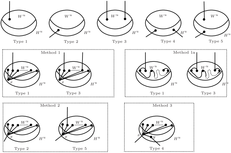
Figure 6: Five types and methods 1, 1a, 2 and 3.

The key to construct $T_{1},\cdots,T_{c}$ is the way of choosing $W^{u}$-Steiner trees $F_{1}^{u},\cdots,F_{c}^{u}$ of $H^{u}$. (We note that if $u$ is not an unlabeled vertex of $G_{s+1}$, then the $F^{u}_{1},\cdots,F^{u}_{c}$ are empty graphs). We have the following five methods to choose.

Method 1 If $F_{i}$ is a graph of Type 1 and $|W^{u}|\geq 2$, or $F_{i}$ is a graph of Type 3, then let $F^{u}_{i}=x\vee W^{u}$, where $x\in R(u)$.

Method 1a If $F_{i}$ is a graph of Type 1 and $|W^{u}|\geq 2$, then let $F^{u}_{i}$ be a Hamiltonian path of $H^{u}[W^{u}]$ such that the vertex in $V_{u,i}$ is an endpoint of this Hamiltonian path; if $F_{i}$ is a graph of type 3, then let $F^{u}_{i}$ be a Hamiltonian path of $H^{u}[W^{u}]$ with the endpoints the two vertices of $V_{u,i}$.

Method 2 If $F_{i}$ is a graph of Type 2 or Type 5, say $x$ is the only vertex of $V_{u,i}$ with $x\notin W^{u}$, then let $F^{u}_{i}=x\vee W^{u}$.

Method 3 If $F_{i}$ is a graph of Type 4, say $V_{u,i}=\{x,y\}$, then let $F^{u}_{i}=xy\cup(x\vee W^{u})$.

Method 4 If $F_{i}$ is a graph of Type 1 and $|W^{u}|=1$. then let $F_{i}^{u}$ be the empty graph.

It is worth noting that the method is deterministic if $F_{i}^{u}$ is a graph of Types 2, 4 and 5, or $F_{i}^{u}$ is a graph of Type 1 and $|W^{u}|=1$. So we can first construct these $F_{i}^{u}$ by using Method 2, Method 3 and Method 4, respectively, and then construct $F^{u}_{i}$ of Type 1 with $|W^{u}|\geq 2$ and Type 3 by using Method 1 or Method 3. Along this process, we have the following result.

Claim 2.

If $|W^{u}|=1$ (say $W^{u}=\{x\}$), then the following statements hold.

1. If $F_{i}$ is not a graph of Type 5, then we can choose $F_{i}^{u}$ such that $d_{T_{i}}(x)=1$.

2. If $F_{i}$ is a graph of Type 5, then we can choose $F_{i}^{u}$ such that $d_{T_{i}}(x)=2$.

Algorithm 1 is an algorithm for finding $c$ $U$-Steiner trees of $G$. For each step of $s$, the algorithm will construct $c$ $U^{s-1}$-steiner trees $T^{\prime}_{1},T^{\prime}_{2},\ldots,T^{\prime}_{c}$. If Arithmetic 1 is correct, then Lines 16-39 indicate that $d_{T^{\prime}}(x)\leq 2$ for any $x\in W^{u}$, and hence ($\star$) always holds. We denote each $T^{\prime}_{i}$ in Line 40 by $T^{u}_{i}$ below.

Remark 2.1.

If $x\in W^{u}$ and there are $p$ $T_{i}^{u}$ such that $d_{T_{i}^{u}}(x)=2$, then $n_{4}(x)\leq p$.

We now check the correctness of the algorithm. Since $F_{i}^{u}$ is deterministic when $u$ is an unlabeled vertex (Lines 5–15 of Algorithm 1), and $F_{i}^{u}$ is deterministic if $F_{i}^{u}$ is a graph of Types 2, 4 and 5, or $F_{i}^{u}$ is a graph of Type 1 and $|W^{u}|=1$ (Lines 16–27 of Algorithm 1), we only need to talk about the labeled vertex $u$ with $|W^{u}|\geq 2$ and check the correctness of Lines 28–35 of Algorithm 1, that is, to ensure that there exists $n_{1}(u)$ $F_{i}^{u}$s of Type 1 and $n_{3}(u)$ $F_{i}^{u}$s of Type 3. If $F_{i}^{u}$ is constructed by Method 1, then $F_{i}^{u}$ is a star with center in $R(u)$ (say the center of the star is $c_{i}$); if $F_{i}^{u}$ is constructed by Method 1a, then $F_{i}^{u}$ is Hamiltonian path of $H^{u}$ with endpoints in $V_{u,i}$. Since $c_{i}$s are pairwise differently and are contained in $R(u)$, and $H^{u}$ has at most $\lfloor|W^{u}|/2\rfloor$ Hamiltonian paths to afford by Corollary 2.2, we only need to ensure that $|R(u)|+\lfloor|W^{u}|/2\rfloor\geq n_{1}(u)+n_{3}(u)$. Since

$$n_{1}(u)+n_{3}(u)-|R(u)| =n_{1}(u)+n_{3}(u)-[\ell-|W^{u}|-n_{2}(u)-2n_{4}(u)-n_{5}(u)]$$

$$=[n_{1}(u)+n_{2}(u)+n_{3}(u)+n_{4}(u)+n_{5}(u)]+n_{4}(u)+|W^{u}|-\ell$$

$$=c+n_{4}(u)+|W^{u}|-\ell.$$

and $c=\ell-\lceil k/2\rceil$, it follows that

$$n_{1}(u)+n_{3}(u)-|R(u)|=n_{4}(u)+|W^{u}|-\lceil k/2\rceil.$$ (1)

Thus, we only need to prove the following result.

Claim 3.

For each labeled vertex $u\in V(\overrightarrow{T})$ with $|W^{u}|\geq 2$, the inequality

$$n_{1}(u)+n_{3}(u)-|R(u)|\leq\lfloor|W^{u}|/2\rfloor$$ (2)

holds.

Before the proof of Claim 3, we give a series of claims as a prelude.

Claim 4.

If $n_{4}(u)\leq 1$ and $2\leq|W^{u}|\leq\left\lceil\frac{k}{2}\right\rceil-1$, then $n_{1}(u)+n_{3}(u)-|R(u)|\leq 0$. Moreover, for each vertex $x\in W^{u}$, there is at most one of $T_{i}^{u}$ such that $d_{T_{i}^{u}}(x)=2$.

Proof.

Since $n_{4}(u)\leq 1$ and $|W^{u}|\leq\left\lceil\frac{k}{2}\right\rceil-1$, it follows from equality (1) that $n_{1}(u)+n_{3}(u)-|R(u)|=|W^{u}|-\left\lceil\frac{k}{2}\right\rceil+1\leq 0.$ By Algorithm 1 (Lines 18–38), each $F_{i}^{u}$ of Type 1 and Type 3 is constructed by using Method 1. Furthermore, for each vertex $x\in W^{u}$, there is at most one $T_{i}^{u}$ such that $d_{T_{i}^{u}}(x)\leq 2$. ∎

Claim 5.

If $n_{4}(u)\leq 1$ and $k-1\geq|W^{u}|\geq\left\lceil\frac{k}{2}\right\rceil$, then $n_{1}(u)+n_{3}(u)-|R(u)|\leq\lfloor|W^{u}|/2\rfloor$. Moreover, for each $x\in W^{u}$,

1. there are at most $|W^{u}|-\left\lceil\frac{k}{2}\right\rceil+2$ $T_{i}^{u}$ such that $d_{T_{i}^{u}}(x)=2$;

2. if $n_{4}(u)=0$, then there are at most $|W^{u}|-\left\lceil\frac{k}{2}\right\rceil+1$ $T_{i}^{u}$ such that $d_{T_{i}^{u}}(x)=2$.

Proof.

Since $n_{4}(u)\leq 1$, it follows that $n_{1}(u)+n_{3}(u)-|R(u)|\leq|W^{u}|-\left\lceil\frac{k}{2}\right\rceil+1$ and the equality indicates $n_{4}(u)=0$. If $|W^{u}|\leq k-2$, then

$$n_{1}(u)+n_{3}(u)-|R(u)|\leq|W^{u}|-\left\lceil(|W^{u}|+2)/2\right\rceil+1\leq\left\lfloor\frac{|W^{u}|}{2}\right\rfloor;$$

if $|W^{u}|=k-1$ and $k$ is even, then

$$n_{1}(u)+n_{3}(u)-|R(u)|\leq|W^{u}|-\left\lceil(|W^{u}|+1)/2\right\rceil+1=\left\lfloor\frac{|W^{u}|+1}{2}\right\rfloor=\left\lfloor\frac{|W^{u}|}{2}\right\rfloor;$$

if $|W^{u}|=k-1$ and $k$ is odd, then

$$n_{1}(u)+n_{3}(u)-|R(u)|\leq(k-1)-\left\lceil k/2\right\rceil+1\leq\left\lfloor k/2\right\rfloor=\left\lfloor(k-1)/2\right\rfloor=\left\lfloor|W^{u}|/2\right\rfloor.$$

Therefore, $n_{1}(u)+n_{3}(u)-|R(u)|\leq\left\lfloor|W^{u}|/2\right\rfloor$. By Algorithm 1 (Lines 18–38), there are $|R(u)|$ $F_{i}^{u}$ of Type 1 and Type 3 constructed by using Method 1, and $n_{1}(u)+n_{3}(u)-|R(u)|$ $F_{i}^{u}$ of Type 1 and Type 3 are constructed by using Method 1a. For each $x\in W^{u}$, there are at most $n_{1}(u)+n_{3}(u)-|R(u)|+1=|W^{u}|-\left\lceil\frac{k}{2}\right\rceil+2$ $T_{i}^{u}$ such that $d_{T_{i}^{u}}(x)=2$, and the equality indicates $n_{4}(u)=1$. Thus, if $n_{4}(u)=0$, then for each vertex $x\in W^{u}$, there are at most $n_{1}(u)+n_{3}(u)-|R(u)|+1=|W^{u}|-\left\lceil\frac{k}{2}\right\rceil+1$ $F_{i}^{u}$ such that $d_{T_{i}^{u}}(x)=2$. ∎

Claim 6.

If $k-1\geq|W^{v}|\geq\left\lceil\frac{k}{2}\right\rceil$ (recall that $v$ is the vertex of $\overrightarrow{T}$ such that $u\in W^{v}$), $2\leq|W^{u}|\leq\left\lceil\frac{k}{2}\right\rceil-1$ and $|W^{u}|+|W^{v}|=k-2+\lambda$, where $\lambda\leq 2$, then $n_{1}(u)+n_{3}(u)-|R(u)|\leq\lfloor|W^{u}|/2\rfloor$ and the following hold.

1. If $\lambda\leq 0$ or $v=v_{root}$, then for each vertex $x\in W^{u}$, there is at most one $T_{i}^{u}$ such that $d_{T_{i}^{u}}(x)=2$.

2. If $v\neq v_{root}$ and $\lambda\in\{1,2\}$, then for each vertex $x\in W^{u}$, there are at most $\lambda+1$ of $T_{i}^{u}$ such that $d_{T_{i}^{u}}(x)=2$.

Proof.

Fact 2.

If $v\neq v_{root}$ and $\lambda=2$, then $n_{1}(u)+n_{3}(u)-|R(u)|\leq\lambda-1$; otherwise, $n_{1}(u)+n_{3}(u)-|R(u)|\leq\lambda$.

Proof.

By Claim 5 (see $v,u$ as the vertices $u,x$ of Claim 5, respectively), we have that $n_{4}(u)\leq|W^{v}|-\lceil k/2\rceil+2$. Note that $|W^{u}|+|W^{v}|=k-2+\lambda$. Then

$$n_{1}(u)+n_{3}(u)-|R(u)| =n_{4}(u)+|W^{u}|-\lceil k/2\rceil$$

$$\leq(|W^{v}|-\lceil k/2\rceil+2)+(k-2+\lambda-|W^{v}|)-\lceil k/2\rceil$$

$$=k-2\lceil k/2\rceil+\lambda\leq\lambda.$$

Thus, we only need to prove that if $v\neq v_{root}$ and $\lambda=2$, then $n_{1}(u)+n_{3}(u)-|R(u)|\leq\lambda-1$.

We first show that if $v\neq v_{root}$ and $\lambda=2$ then $n_{4}(u)\leq|W^{v}|-\lceil k/2\rceil+1$. Note that $|W^{u}|+|W^{v}|+|W^{v_{root}}|\leq k+2$ by Fact 1. Since $|W^{v}|+|W^{u}|=k$ and $|W^{v_{root}}|\geq 2$, it follows that $|W^{v_{root}}|=2$ (say $W^{v_{root}}=\{z_{1},z_{2}\}$). By Claim 1, we have that $d_{T_{i}^{v_{root}}}(z_{j})=1$ for each $j\in\{1,2\}$ and $i\in\{1,\ldots,c\}$. Hence, if $v\in W^{v_{root}}$, then $d_{T_{i}^{v_{root}}}(v)=1$ for each $i\in[c]$, which implies that $n_{4}(v)=0$. By Claim 5, we have that $n_{4}(u)\leq|W^{v}|-\lceil k/2\rceil+1$. Thus, suppose $v\notin W^{v_{root}}$ (without loss of generality, suppose $v_{root}\overrightarrow{T}v=v_{root}v_{1}v_{2}\ldots v_{p}v$). By Fact 1, $|W^{v_{i}}|=1$ for each $i\in\{1,\ldots,p\}$. Recall that $d_{T_{i}^{v_{root}}}(z_{j})=1$ for each $j\in\{1,2\}$ and $i\in\{1,\ldots,c\}$. By Claim 2, we have that $n_{4}(v_{1})=0$. Furthermore, we get that $n_{4}(v_{1})=\ldots=n_{4}(v_{p})=n_{4}(v)$ by a recursive process. So, by Claim 5, $n_{4}(u)\leq|W^{v}|-\lceil k/2\rceil+1$. Therefore, we proved that $n_{4}(u)\leq|W^{v}|-\lceil k/2\rceil+1$. Using this inequality, we have that

$$n_{1}(u)+n_{3}(u)-|R(u)| =n_{4}(u)+|W^{u}|-\lceil k/2\rceil$$

$$\leq(|W^{v}|-\lceil k/2\rceil+1)+(k-|W^{v}|)-\lceil k/2\rceil$$

$$\leq 1=\lambda-1.$$

Thus the proof is complete. ∎

Suppose $\lambda\leq 0$ or $v=v_{root}$. If $\lambda\leq 0$, then by Fact 2, $n_{1}(u)+n_{3}(u)-|R(u)|\leq 0$; if $v=v_{root}$, then $n_{4}(u)\leq|W^{v}|-\lceil k/2\rceil$ by Claim 1, and hence

$$n_{1}(u)+n_{3}(u)-|R(u)| =n_{4}(u)+|W^{u}|-\lceil k/2\rceil\leq(|W^{v}|-\lceil k/2\rceil)+(k-|W^{v}|)-\lceil k/2\rceil\leq 0.$$

Therefore, $n_{1}(u)+n_{3}(u)-|R(u)|\leq 0$. By Algorithm 1 (Lines 18–38), each $F_{i}^{u}$ of Type 1 and Type 3 is constructed by using Method 1. Hence, for each vertex $x\in W^{u}$, there is at most one $T_{i}^{u}$ such that $d_{T_{i}^{u}}(x)=2$.

Input: $U$, $c$ and $G=S(n,\ell)$ with $|W^{root}|\geq 2$

Output: $c$ $U$-Steiner trees $T^{\prime}_{1},T^{\prime}_{2},\ldots,T^{\prime}_{c}$ of $G$

1$T^{\prime}_{1},T^{\prime}_{2},\ldots,T^{\prime}_{c}$ are empty graphs;

2$s=n$ //(* $n$ is the minimum dimension such labeled vertex all in $S(n,\ell)$ *);

3 for $s\geq 1$ do

4       for each vertex $u$ of $G_{s}$ do

5             if  $u$ is an unlabeled vertex then

6                   for  $1\leq i\leq c$ do

7                         if  $u$ is a vertex of $F_{i}$ then

8                               $F_{i}^{u}$ is a spanning tree of $H^{u}$;

9                        else

10                               $\ F_{i}^{u}$ is is the empty graph;

11                         end if

12                        $T^{\prime}_{i}=T^{\prime}_{i}\cup F_{i}^{u}$;

13                         $i=i+1$;

14                        

15                   end for

16                  

17             end if

18            

19            if  $u$ is a labeled vertex then

20                   $\mu=|R(u)|$;

21                   for  $1\leq i\leq c$ do

22                        

23                        if  $T^{\prime}_{i}$ is of Type 2 or Type 5 then

24                               construct $F_{i}^{u}$ by using Method 2;

25                         end if

26                        

27                        if  $T^{\prime}_{i}$ is of Type 4 then

28                               construct $F_{i}^{u}$ by using Method 3;

29                         end if

30                        

31                        if  $T^{\prime}_{i}$ is of Type 1 and $|W^{u}|=1$ then

32                               construct $F_{i}^{u}$ by using Method 4;

33                         end if

34                        

35                        if  either $T^{\prime}_{i}$ is of Type 1 and $|W^{u}|\geq 2$, or $T^{\prime}_{i}$ is of Type 3 then

36                               if  $\mu>0$ then

37                                     construct $F_{i}^{u}$ by using Method 1; $\mu=\mu-1$;

38                               end if

39                              

40                              if  $\mu\leq 0$ then

41                                     construct $F_{i}^{u}$ by using Method 1a;

42                               end if

43                              

44                         end if

45                        

46                        $T^{\prime}_{i}=T^{\prime}_{i}\cup F_{i}^{u}$;

47                         $i=i+1$;

48                        

49                   end for

50                  

51             end if

52            

53       end for

54      $s=s-1$;

55      

56 end for

Algorithm 1 The construction of $c$ $U$-Steiner trees of $G$

Suppose $v\neq v_{root}$ and $\lambda\in\{1,2\}$. Then by Fact 2, $n_{1}(u)+n_{3}(u)-|R(u)|\leq 1\leq\lfloor|W^{u}|/2\rfloor$. By Algorithm 1 (Lines 18–38), there are $|R(u)|$ $F_{i}^{u}$ of Type 1 and Type 3 are constructed by using Method 1, and $n_{1}(u)+n_{3}(u)-|R(u)|$ $F_{i}^{u}$ of Type 1 and Type 3 are constructed by using Method 1a. Thus, for each vertex $x\in W^{u}$, there are at most $n_{1}(u)+n_{3}(u)-|R(u)|+1\leq\lambda+1$ $F_{i}$ such that $d_{T_{i}^{u}}(x)=2$. ∎

Claim 7.

If $|W^{v}|,|W^{u}|\geq\left\lceil\frac{k}{2}\right\rceil$ and $|W^{v}|+|W^{u}|\neq k+1$, then $n_{1}(u)+n_{3}(u)-|R(u)|\leq\lfloor|W^{u}|/2\rfloor$ and the following hold.

1. If $v=v_{root}$, then for each vertex $x\in W^{u}$, there is at most one of $T_{i}^{u}$ such that $d_{T_{i}^{u}}(x)=2$.

2. If $v\neq v_{root}$, then for each vertex $x\in W^{u}$, there are at most two of $T_{i}^{u}$ such that $d_{T_{i}^{u}}(x)=2$.

Proof.

If $k$ is odd, or $k$ is even and one of $|W^{u}|$ and $|W^{v}|$ is greater than $k/2$, then $|W^{u}|+|W^{v}|=k+1$, a contradiction. Therefore, $k$ is even and $|W^{v}|=|W^{u}|=k/2$.

Suppose $v=v_{root}$. Then by Claim 1, $n_{4}(u)=0$. Thus,

$$n_{1}(u)+n_{3}(u)-|R(u)|=n_{4}(u)+|W^{u}|-k/2=|W^{u}|-k/2=0.$$

By Algorithm 1 (Lines 18–38), each $F_{i}^{u}$ of Type 1 and Type 3 is constructed by using Method 1. Moreover, for each vertex $x\in W^{u}$, there is at most one $T_{i}^{u}$ such that $d_{T_{i}^{u}}(x)=2$.

Suppose $v\neq v_{root}$. If $v\in W^{v_{root}}$, then by Claims 1 and 5, we have that $n_{4}(u)\leq|W^{u}|-k/2+1$; if $v\notin W^{v_{root}}$ (without loss of generality, suppose $v_{root}\overrightarrow{T}v=v_{root}v_{1}v_{2}\ldots v_{p}v$), then by Fact 1, $|W^{root}|=2$ and $|W^{v_{i}}|=1$ for each $i\in\{1,\ldots,p\}$. By Claim 1, $d_{T_{i}^{v_{root}}}(v_{1})=1$. By Claim 2, we have that $n_{4}(v_{1})=0$. Furthermore, we get that $n_{4}(v_{1})=\ldots=n_{4}(v_{p})=n_{4}(v)$ by a recursive process. Hence, $n_{4}(u)\leq|W^{v}|-k/2+1$ by Claim 5. So, $n_{4}(u)\leq|W^{v}|-k/2+1$ and

$$n_{1}(u)+n_{3}(u)-|R(u)|=n_{4}(u)+|W^{u}|-k/2=1\leq\lfloor|W^{u}|/2\rfloor.$$

By Algorithm 1 (Lines 18–38), there are $|R(u)|$ $F_{i}^{u}$ of Type 1 and Type 3 are constructed by using Method 1, and $n_{1}(u)+n_{3}(u)-|R(u)|$ $F_{i}^{u}$ of Type 1 and Type 3 are constructed by using Method 1a. For each vertex $x\in W^{u}$, it is obvious that there are at most two $T_{i}^{u}$ such that $d_{T_{i}^{u}}(x)=2$. ∎

Suppose $\mathfrak{S}=\{z\in V(\overrightarrow{T}):z\mbox{ is a labeled vertex and }|W^{z}|\geq\lceil k/2\rceil\}$.

Claim 8.

Suppose $a,b\in V(\overrightarrow{T})$, $a\prec b$ and $V(\overrightarrow{T}-a)\cap\mathfrak{S}=\emptyset$. If either $|W^{a}|=1$ or $a\notin\mathfrak{S}$ and $n_{4}(a)\leq 1$, then for each $z\in V(a\overrightarrow{T}b)-a$, $n_{4}(z)\leq 1$.

Proof.

Without loss of generality, suppose $a\overrightarrow{T}b=az_{1}z_{2}\ldots z_{p}b$. If $|W^{a}|=1$, then $n_{4}(a)\leq 1$ by Claim 2. Therefore, $n_{4}(a)\leq 1$. If $|W^{z_{1}}|=1$, then by Claim 2, $n_{4}(z_{1})\leq 1$. If $|W^{z_{1}}|\geq 2$, then by Claim 4, there are at most one of $T_{i}^{a}$ such that $d_{T_{i}^{a}}(z_{1})=2$. Hence, $n_{4}(z)\leq 1$. Since $z_{2}\notin\mathfrak{S}$ and $n_{4}(z_{1})\leq 1$, it follows that $n_{4}(z_{2})\leq 1$. Repeat this progress, we can get that the result holds. ∎

Proof of Claim 3: Suppose $v^{*}$ is the maximum vertex of $v_{root}\overrightarrow{T}u$ such that either $|W^{v^{*}}|=1$ or $2\leq|W^{v^{*}}|\leq\lceil k/2\rceil-1$ and $n_{4}(v^{*})\leq 1$.

Case 1.

$v^{*}$ exists.

Let $\overrightarrow{P}=v^{*}\overrightarrow{T}u=v^{*}z_{1}z_{2}\ldots z_{p}u$. If $|\overrightarrow{P}|=1$, then $\overrightarrow{P}=u$. Since $|W^{u}|\geq 2$, it follows that $2\leq|W^{u}|\leq\lceil k/2\rceil-1$ and $n_{4}(u)\leq 1$, and hence $n_{1}(u)+n_{3}(u)-|R(u)|\leq 0$, the inequality (2) holds. Thus, suppose $|\overrightarrow{P}|\geq 2$. Since $u\in W^{v}$, it follows that $v\in V(\overrightarrow{P})$. By Claim 8, $n_{4}(z_{1})\leq 1$. Thus, by the maximality of $v^{*}$, we have that $|W^{z_{1}}|\geq\lceil k/2\rceil$.

Subcase 1.1.

$v=v^{*}$.

Then $u=z_{1}$. Since $n_{4}(z_{1})\leq 1$ and $|W^{u}|\geq\lceil k/2\rceil$, it follows from Claim 5 that $n_{1}(u)+n_{3}(u)-|R(u)|\leq\lfloor|W^{u}|/2\rfloor$, the inequality (2) holds.

Subcase 1.2.

$v=z_{1}$.

Then $u=z_{2}$. By Fact 1, we have that $|W^{z_{1}}|+|W^{z_{2}}|+|W^{v_{root}}|-2\leq k$. Hence, $|W^{z_{1}}|\leq k-2$ and $|W^{z_{1}}|+|W^{z_{2}}|\leq k$. Note that $v=z_{1}$ and $|W^{z_{1}}|\geq\lceil k/2\rceil$. If $2\leq|W^{u}|\leq\lceil k/2\rceil-1$, then by Claim 6, we have that $n_{1}(u)+n_{3}(u)-|R(u)|\leq\lceil|W^{u}|/2\rceil$. If $|W^{u}|\geq\lceil k/2\rceil$, then by Claim 7, we have that $n_{1}(u)+n_{3}(u)-|R(u)|\leq\lfloor|W^{u}|/2\rfloor$. Therefore, the inequality (2) holds.

Subcase 1.3.

$v\succeq z_{2}$.

Then $u\succeq z_{3}$. By the choice of $v^{*}$, we have that $|W^{z_{i}}|\geq 2$ for each $i\in[p]$. Since

$$|W^{v_{root}}|+|W^{z_{1}}|+|W^{z_{2}}|+|W^{z_{3}}|-3\leq k$$ (3)

and $|W^{z_{1}}|\geq\lceil k/2\rceil$, it follows that $|W^{z_{2}}|,|W^{z_{3}}|\leq\lceil k/2\rceil-1$ and $|W^{z_{1}}|+|W^{z_{2}}|\leq k-1=k-2+\lambda$, where $\lambda=1$. Hence, by the maximality of $v^{*}$, we have that $n_{4}(z_{3})\geq 2$. By Claim 6 (here, we can see $z_{1}$ and $z_{2}$ as the vertices $v$ and $u$ in Claim 6, respectively, and then $z_{3}$ can be seen as the vertex $x$ in Claim 6), we have that $|W^{z_{1}}|+|W^{z_{2}}|=k-1$ and $n_{4}(z_{3})\leq\lambda+1=2$. Since $n_{4}(z_{3})\geq 2$, we have that $n_{4}(z_{3})=2$. Since $|W^{v_{root}}|,|W^{z_{3}}|\geq 2$, it follows form the inequality (3) that $|W^{v_{root}}|=|W^{z_{3}}|=2$. Since $|W^{z_{3}}|\leq\lceil k/2\rceil-1$ and $|W^{z_{3}}|=2$, we have that $k\geq 5$. Therefore,

$$n_{1}(z_{3})+n_{3}(z_{3})-|R(z_{3})|=n_{4}(z_{3})+|W^{z_{3}}|-\lceil k/2\rceil\leq 1.$$

If $u=z_{3}$, then the inequality (2) holds. If $u\succ z_{3}$, then $u\succeq z_{4}$ and $|W^{u}|=1$ by Fact 1, which contradicts the choice of $v^{*}$.

Case 2.

$v^{*}$ does not exist.

Suppose $\overrightarrow{P}=v_{root}\overrightarrow{T}u=v_{root}z_{1}\ldots,z_{q}u$. For each vertex $z\in V(\overrightarrow{P})$, either $2\leq|W^{z}|\leq\lceil k/2\rceil-1$ and $n_{4}(z)\geq 2$, or $|W^{z}|\geq\lceil k/2\rceil$. Since $n_{4}(v_{root})=0$, it follows that $|W^{v_{root}}|\geq\lceil k/2\rceil$. By Claim 1, $n_{4}(z_{1})\leq|W^{v_{root}}|-\lceil k/2\rceil$.

Subcase 2.1.

$|W^{z_{1}}|\geq\lceil k/2\rceil$.

Since $|W^{v_{root}}|,|W^{z_{1}}|\geq\lceil k/2\rceil$, we have that $t\leq 1$. Otherwise, $\sum_{z\in V(\overrightarrow{P})}|W^{z}|-(|\overrightarrow{P}|-1)>k$, which contradict Fact 1. Moreover, if $t=1$, then $k$ is even, $|W^{v_{root}}|=|W^{z_{1}}|=k/2$ and $|W^{u}|=2$.

Suppose $v=v_{root}$. Then $u=z_{1}$ and $n_{4}(u)\leq|W^{v_{root}}|-\lceil k/2\rceil$ by Claim 1. Thus,

$$n_{1}(u)+n_{3}(u)-|R(u)|=n_{4}(u)+|W^{u}|-\lceil k/2\rceil\leq 1=\lfloor|W^{u}|/2\rfloor,$$

the inequality (2) holds.

Suppose $v\neq v_{root}$. Then $\overrightarrow{P}=v_{root}z_{1}u$ and $v=z_{1}$, and $|W^{v_{root}}|+|W^{z_{1}}|\leq k$. By Claim 7 (here, we see $v_{root}$ and $v=z_{1}$ as the vertices $v$ and $u$ in Claim 7, respectively, and then $u$ can be seen as the vertex $x$ in Claim 7), we have that $n_{4}(u)\leq 1$. Hence,

$$n_{1}(u)+n_{3}(u)-|R(u)|=n_{4}(u)+|W^{u}|-\lceil k/2\rceil\leq 1\leq\lfloor|W^{u}|/2\rfloor,$$

the inequality (2) holds.

Subcase 2.2.

$2\leq|W^{z_{1}}|\leq\lceil k/2\rceil-1$.

Recall that $n_{4}(z_{1})=|W^{v_{root}}|-\lceil k/2\rceil$. If $|W^{v_{root}}|+|W^{z_{1}}|=k+1$, then $v=v_{root}$, $u=z_{1}$ and $n_{1}(u)+n_{3}(u)-|R(u)|\leq 1\leq\lfloor|W^{u}|/2\rfloor.$ Thus, suppose $|W^{v_{root}}|+|W^{z_{1}}|\leq k$. Then

$$n_{1}(z_{1})+n_{3}(z_{1})-|R(z_{1})|=n_{4}(z_{1})+|W^{z_{1}}|-\lceil k/2\rceil\leq 0,$$

and hence $n_{4}(z_{2})\leq 1$, which implies that either $z_{1}=u$ or $z_{2}$ exists and $|W^{z_{2}}|\geq\lceil k/2\rceil$. If $z_{1}=u$, then $n_{1}(u)+n_{3}(u)-|R(u)|\leq 0$, the inequality (2) holds. If $z_{2}$ exists and $|W^{z_{2}}|\geq\lceil k/2\rceil$, then by Fact 1 and the existence of $v^{*}$, $z_{2}=u$ and hence $n_{4}(u)\leq 1$. Furthermore, we get that $n$ is even, $|W^{u}|=|W^{v_{root}}|=k/2$ and $|W^{z_{1}}|=2$. Thus,

$$n_{1}(u)+n_{3}(u)-|R(u)|\leq 1+|W^{u}|-k/2=1\leq\lfloor|W^{u}|/2\rfloor,$$

and the inequality (2) holds. ∎

Proof of Theorem 1.3: We first consider $3\leq k\leq\ell$. The lower bound $\ell-\lceil k/2\rceil\leq\kappa_{k}(S(n,\ell))\leq\lambda_{k}(S(n,\ell))$ can be obtained from Theorem 2.3 directly. For the upper bounds of $\kappa_{k}(S(n,\ell))$ and $\lambda_{k}(S(n,\ell))$, consider the graph $G_{n-1}$. Let $V(G_{n-1})=\{u_{1},\ldots,u_{\ell}\}$, $U=\{x_{1},\ldots,x_{k}\}$ and $x_{i}\in A_{n-1,u_{i}}$, where $k\leq\ell$. Suppose there are $p$ edge-disjoint $U$-Steiner trees $T^{\prime}_{1},\ldots,T^{\prime}_{p}$ of $G=S(n,\ell)$ and $\mathcal{P}=\{A_{n-1,u}:u\in V(G_{n-1})\}$. Let $T^{*}_{i}=T^{\prime}_{i}/\mathcal{P}$ for $i\in[p]$. Then $T^{*}_{1},\ldots,T^{*}_{p}$ are edge-disjoint connected graphs of $G_{n-1}$ containing $\{u_{1},\ldots,u_{k}\}$. Thus, $p\leq\lambda_{k}(G_{n-1})=\lambda_{k}(K_{\ell})=\ell-\lceil k/2\rceil$. Therefore, $\kappa_{k}(S(n,\ell))\leq\lambda_{k}(S(n,\ell))\leq\ell-\lceil k/2\rceil$, the upper bound follows.

Now consider the case $\ell+1\leq k\leq{\ell}^{n}$. By Theorem 1.2, $\lambda_{k}(S(n,\ell))\geq\lfloor\ell/2\rfloor$. Since $\lambda_{k}(S(n,\ell))\leq\lambda_{\ell}(S(n,\ell))=\lfloor\ell/2\rfloor$, it follows that $\kappa_{k}(S(n,\ell))\leq\lambda_{k}(S(n,\ell))\leq\lfloor\ell/2\rfloor$. Therefore, $\lambda_{k}(S(n,\ell))=\lfloor\ell/2\rfloor$ and $\kappa_{k}(S(n,\ell))\leq\lfloor\ell/2\rfloor$. The proof is completed.

3 Some network properties

Generalized connectivity is a graph parameter to measure the stability of networks. In the following part, we will compare the following other parameters of Sierpiński graphs with their generalized connectivity.

Our network is obtained after $t$ iteration as $S(t,\ell)$ that has $N_{t}$ nodes and $E_{t}$ edges, where $t=0,1,2,\cdots,T-1$, and $T$ is the total number of iterations, and our generation process can be illustrated as follows.

Figure 7: The Function of $E_{t}$ and $N_{t}$

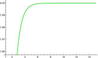
Figure 8: The Average distribution

Step 1: Initialization. Set $t=0$, $G_{1}$ is a complete graph of order $\ell$, and thus $N_{1}=\ell$ and $E_{1}=\binom{\ell}{2}$. Set $G_{1}=S(1,\ell)$.

Step 2: Generation of $G_{t+1}$ from $G_{t}$. Let $S^{1}(t,\ell),S^{2}(t,\ell),\ldots,S^{\ell}(t,\ell)$ be all Sierpiński graphs $S(t,\ell)$ added at Step $t$. At Step $t+1$, we add one edge (bridge edge) between $S^{i}(t,\ell)$ and $S^{j}(t,\ell)$, $i\neq j$, namely the edge between vertices $\langle ij\cdots j\rangle$ and $\langle ji\cdots i\rangle$.

For Sierpiński graphs $G_{t}=S(t,\ell)$, its order and size are $N_{t}=\ell^{t}$ and $E_{t}=\frac{\ell^{t+1}-\ell}{2}$, respectively; see Table 2 and Figure 8; see Figure 8 for the average degree distribution.

Table 2: The size and order of $G_{t}$ for $\ell=3$

$t$	1	2	3	4	5	6	t
$N_{t}$	3	9	27	81	242	729	$\ell^{t}$
$E_{t}$	3	12	39	120	363	1092	$\frac{\ell^{t+1}-\ell}{2}$

The degree distribution for $t$ times are

$$\left(\underbrace{\ell-1,\ell-1,\cdots,\ell-1}_{\ell-1},\underbrace{\ell,\ell,\ell,\cdots,\ell}_{\ell^{t}-\ell}\right).$$ (4)

From Equation 4, the instantaneous degree distribution is $P(\ell-1,t)=(\ell-1)/\ell^{n}$ for $t=1,2,\cdots,T$ and $P(\ell,t)=(\ell^{t}-\ell)/\ell^{n}$ for $t=1,2,\cdots,T$. Note that the density of Sierpiński graphs is $\rho=E_{t}/\binom{N_{t}}{2}$. For any $1\leq k\leq\ell$ we have $|\{v\in V(G)|d_{S(t,\ell)}(v)|\geq k\}\approx|V(S(t,\ell))|$.

Theorem 3.1.

[KlavarS2018] If $n\in\mathbb{N}$ and $G$ is a graph, then $\kappa\left(S(n,G)\right)=\kappa(G)$ and $\lambda\left(S(n,G)\right)=\lambda(G)$.

From Theorem 3.1, we have $\kappa\left(S(n,\ell)\right)=\kappa(K_{\ell})=\ell-1$ and $\lambda\left(S(n,\ell)\right)=\lambda(K_{\ell})=\ell-1$. Note that $\lambda_{k}(S(n,\ell))=\ell-\left\lceil k/2\right\rceil$ and $\kappa_{k}(S(n,\ell))=\ell-\left\lceil k/2\right\rceil$; see Figure 9.

Figure 9: The generalized (edge-)connectivity

of $S(n,\ell)$

As an application of generalized (edge-)connectivity of $S(n,\ell)$, we use the entropy of Steiner trees, which is called the asymptotic complexity; see [7].

Let $\tau(G)$ be the number of spanning tree.

$$\rho(G)=\lim_{V(G)\longrightarrow\infty}\frac{\ln|\tau(G)|}{\left|V(G)\right|}$$ (5)

where $\rho(G)$ is called the entropy of spanning trees or the asymptotic complexity [2].

Similarly to the Equation 5, we give the entropy of the $k$-Steiner tree of a graph $G$ can be defined as

$$\rho_{k}(G)=\lim_{|V(G)|\longrightarrow\infty}\frac{\ln|\kappa_{k}(G)|}{\left|V(G)\right|}$$

The entropy of the $3,4,5$-Steiner tree of Sierpiński graph $S(8,\ell)$ can be seen in Figure 10.

Figure 10: Entropy for $n=8$, $k=3,4,5$

The definition of clustering coefficient can be found in [3]. Let $N_{v}(t)$ be the number of edges in $G_{t}$ among neighbors of $v$, which is the number of triangles connected to the vertex $v$. The clustering coefficient of a graph is based on a local clustering coefficient for each vertex

$$C(v)=\frac{N_{v}(t)}{d_{G}(v)(d_{G}(v)-1)/2},$$

If the degree of node $i$ is $0$ or $1$, then we can set $C_{i}=0$. By definition, we have $0\leq C_{i}\leq 1$.

The clustering coefficient for the whole graph is the average of the local values $C_{i}$

$$C=\frac{1}{|V(G)|}\sum_{i=1}^{n}C_{i}$$

where $n$ is the number of vertices in the network. The clustering coefficient of a graph is closely related to the transitivity of a graph, as both measure the relative frequency of triangles.

Proposition 3.1.

The clustering coefficient of generalized Sierpiński graph $S(n,\ell)$ is

$$C(S(n,\ell))=\frac{\ell^{-n}\left(-2\ell+\ell^{n}+\ell^{n+1}\right)}{\ell-1}.$$

Proof.

For any $v\in V(S(n,\ell))$, if $v$ is a extremal vertex, then $d_{S(n,\ell)}(v)=\ell-1$ and $G[\{N(v)\}]\cong K_{\ell}$, and hence

$$C(v)=\frac{N_{v}(t)}{d_{G}(v)(d_{G}(v)-1)/2}={\binom{\ell}{2}}/{\binom{\ell}{2}}=1.$$

If $v$ is not a extremal vertex, then $d_{S(n,\ell)}(v)=\ell$ and $G[\{N(v)\}]\cong K_{\ell}+e$, where $K_{\ell}+e$ is graph obtained from a complete graph $K_{\ell}$ by adding a pendent edge. Hence, we have $C(v)={\binom{\ell+1}{2}}/{\binom{\ell}{2}}=\frac{\ell+1}{\ell-1}$.

Since there exists $\ell$ extremal vertices in Sierpiński graph $S(n,\ell)$, it follows that

$$C=\frac{1}{|V(G)|}\sum_{i=1}^{n}C_{i}=\frac{1}{\ell^{n}}\left({\ell\times 1+(\ell^{n}-\ell)\frac{\ell+1}{\ell-1}}\right)=\frac{\ell^{-n}\left(-2\ell+\ell^{n}+\ell^{n+1}\right)}{\ell-1}$$

∎

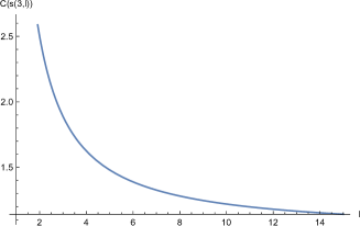
Figure 11: The Function of $C(S(3,l))$

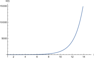
Figure 12: The diameter of $S(n,\ell)$

Theorem 3.2.

[21] The diameter of $S(n,\ell)$ is $Diam(S(n,\ell))=2^{\ell}-1$;

For network properties of Sierpiński graph $S(n,\ell)$, the the diameter function can be seen in Figure 12 and its clustering coefficient is closely related to $1$ when $\ell\longrightarrow\infty$; see Figure 12, which implies that the Sierpiński graph $S(n,\ell)$ is a hight transitivity graph.

References

- [1] J.A. Bondy, U.S.R. Murty, Graph Theory, GTM 244, Springer, 2008.
- [2] R. Burton, R. Pemantle, Local characteristics, entropy and limit theorems for spanning trees and domino tilings via transfer-impedances, Annals of Probability,21(1993),3 1329–1371.
- [3] B. Bollobás, O.M. Riordan, Mathematical results on scale-free random graphs, in: S. Bornholdt, H.G. Schuster (Eds.), Handbook of Graphs and Networks: From the Genome to the Internet, Wiley-VCH, Berlin, 2003, 1–34.
- [4] G. Chartrand, F. Okamoto, P. Zhang, Rainbow trees in graphs and generalized connectivity, Networks 55(4) (2010), 360–367.
- [5] B.L. Chen, K.C. Huange, On the Line -arboricity of and , Discrete Math. 254 (2002), 83–87.
- [6] X. Cheng, D. Du, Steiner trees in Industry, Kluwer Academic Publisher, Dordrecht, 2001.
- [7] M. Dehmer, F. Emmert-Streib, Z. Chen, X. Li, and Y. Shi, Mathematical foundations and applications of graph entropy, John Wiley Sons. (2017).
- [8] D. Du, X. Hu, Steiner tree problems in computer communication networks, World Scientific, 2008.
- [9] C. Hao, W. Yang, The generalized connectivity of data center networks. Parall. Proce. Lett. 29 (2019), 1950007.
- [10] J. Gu, J. Fan, Q. Ye, L. Xi, Mean geodesic distance of the level- Sierpiński gasket, J. Math. Anal. Appl. 508(1) (2022), 125853.
- [11] S. Klavz̆ar, U. Milutinović, Graphs and a variant of tower of hanoi problem, Czechoslovak Math. J. 122(47) (1997), 95–104.
- [12] H. Li, X. Li, and Y. Sun, The generalied -connectivity of Cartesian product graphs, Discrete Math. Theor. Comput. Sci., 14(1) (2012), 43–54.
- [13] H. Li, Y. Ma, W. Yang, Y. Wang, The generalized -connectivity of graph products, Appl. Math. Comput. 295 (2017), 77–83.
- [14] S. Li, J. Tu, C. Yu, The generalized -connectivity of star graphs and bubble-sort graphs, Appl. Math. Comput. 274(1) (2016), 41–46.
- [15] X. Li, Y. Mao, Generalized Connectivity of Graphs, Springer Briefs in Mathematics, Springer, Switzerland, 2016.
- [16] X. Li, Y. Mao, Y. Sun, On the generalized (edge-)connectivity of graphs, Australasian J. Combin. 58(2) (2014), 304–319.
- [17] Y. Li, Y. Mao, Z. Wang, Z. Wei, Generalized connectivity of some total graphs, Czechoslovak Math. J. 71 (2021), 623–640.
- [18] C. Li, S. Lin, S. Li, The -set tree connectivity of -star networks. Theore. Comput. Sci. 844 (2020), 81–86.
- [19] S. Lin, Q. Zhang, The generalized -connectivity of hypercubes. Discrete Appl. Mathe. 220 (2017), 60–67.
- [20] H. Li, X. Li, Y. Sun, The generalized -connectivity of Cartesian product graphs, Discrete Math. Theor. Comput. Sci. 14 (2012), 43–54.
- [21] D. Parisse, On some metric properties of the the Sierpiński graphs . Ars Comb. (2009)90, 145–160
- [22] A. Sahu, A. Priyadarshi, On the box-counting dimension of graphs of harmonic functions on the Sierpiński gasket. Journal of Mathe. Analy. and Appl., 487(2) (2020), 124036.
- [23] B. Xue, L. Zuo, G. Li, The hamiltonicity and path -coloring of Sierpiński-like graphs, Discrete Appl. Math. 160 (2012), 1822–836.
- [24] B. Xue, L. Zuo, On the linear -arboricity of , Discrete Appl. Math 158 (2010) 1546–1550.
- [25] S. Zhao, R. Hao, L. Wu, The generalized connectivity of -bubble-sort graphs. The Comput. Jour., 62 (2019), 1277–1283.
- [26] S. Zhao, R. Hao, J. Wu, The generalized -connectivity of some regular networks, J. Parall. Distr. Comput. 133 (2019), 18–29.
- [27] S. Zhao, R. Hao, The generalized connectivity of alternating group graphs and -star graphs, Discrete Appl. Math. 251 (2018), 310–321.
- [28] S. Zhao, R. Hao, E. Cheng, Two kinds of generalized connectivity of dual cubes, Discrete Appl. Math. 257 (2019), 306–316.
- [29] S. Zhao, R. Hao, The generalized connectivity of alternating group graphs and -star graphs, Discrete Appl. Math. 251 (2018), 310–321.
- [30] S. Zhao, R. Hao, The generalized -connectivity of exchanged hypercubes, Applied Mathe. Comput. 347 (2019), 342–353.
- [31] S. Zhao, R. Hao, J. Wu, The generalized -connectivity of hierarchical cubic networks, Discrete Appl. Mathe., 289 (2021), 194–206.
- [32] S. Zhao, J. Chang, Z. Li, The generalized -connectivity of pancake graphs, Discrete Appl. Math. 327 (2023), 77–86.
- [33] S. Zhao, R. Hao, The generalized -connectivity of exchanged hypercubes. Appl. Math. Comput. 347 (2019), 342–353.