Demonstration and frequency noise characterization of a $17$ µm quantum cascade laser

Abstract

We describe the properties of a continuous-wave room-temperature quantum cascade laser operating at the long wavelength of 17 µm. Long wavelength mid-infrared quantum cascade lasers offer new opportunities for chemical detection, vibrational spectroscopy and metrological measurements using molecular species. In particular, probing low energy vibrational transitions would be beneficial to the spectroscopy of large and complex molecules, reducing intramolecular vibrational energy redistribution which acts as a decoherence channel. By performing linear absorption spectroscopy of the v₂ fundamental vibrational mode of N2O molecules, we have demonstrated the spectral range and spectroscopic potential of this laser, and characterized its free-running frequency noise properties. Finally, we also discuss the potential application of this specific laser in an experiment to test fundamental physics with ultra-cold molecules.

Stimulated by the invention of the quantum cascade laser (QCL) Faist et al. (1994), applications relying on mid-infrared (MIR) radiations have progressed at a very rapid pace in recent years. These range from free-space optical communications Corrigan et al. (2009); Liu et al. (2019); Corrias et al. (2022), gas sensing Nikodem and Wysocki (2012); Daghestani et al. (2014); Martín-Mateos et al. (2017); Robinson et al. (2021) and trace detection Galli et al. (2016), and high-resolution spectroscopy Bielsa et al. (2008); Asselin et al. (2017); Borri et al. (2019); D’Ambrosio et al. (2019), to metrology and frequency referencing Bielsa et al. (2007); Sow et al. (2014); Hansen et al. (2015); Argence et al. (2015); Insero et al. (2017); Santagata et al. (2019), as well as fundamental physics measurements Mejri et al. (2015); Cournol et al. (2019); Lukusa Mudiayi et al. (2021). Unlike MIR gas lasers, such as CO and CO₂ lasers, QCLs can provide broad and continuous frequency tuning over several hundreds of gigahertz. QCLs are also compact, robust and low-power devices compared to other more complex MIR sources based on frequency down conversion Petrov (2012); Schliesser et al. (2012), such as optical parametric generators (OPG), oscillators (OPO) Leindecker et al. (2011), or difference frequency generators (DFG) Sotor et al. (2018); Lamperti et al. (2020), less suited for field deployment. Moreover, QCLs can be easily interchanged and available wavelengths cover large parts of the MIR region from 2.6 Cathabard et al. (2010) to 28 $\mu$m Ohtani et al. (2016), which is not the case of most of the other MIR sources, fiber Jackson and Jain (2020) or crystalline (Cr:ZnSe, Tb:KPb₂Cl₅) MIR lasers Vasilyev et al. (2016)are for example limited to the 2 to 5$\mu$m spectral region.

Distributed feedback (DFB) QCLs Faist et al. (1997), which have a grating embedded in the laser cavity, are single longitudinal mode narrow-band lasers, and thus a solution of choice for molecular spectroscopy. However, until recently continuous wave (CW) DFB QCLs operating at room temperature were only available in the 4 to 11 $\mu$m window. Extending such technologies to longer wavelengths is important for a range of applications: (i) strong vibrational signatures of small hydrocarbons (such as ethene, ethane, acetylene, propane), of larger aromatics (such as BTEX – benzene, toluene, ethylbenzene, and xylenes), of nitrous oxide or uranium hexafluoride are found in the 12-18 $\mu$m spectral window Pirali et al. (2006); Huang et al. (2011); Fuchs et al. (2011); Lamperti et al. (2020); Elkhazraji et al. (2023a, b); in particular, it hosts the strongest absorption lines of C₂H₂, BTEX and UF₆; (ii) long wavelength (N and Q astronomical bands) QCLs would be valuable in radio-astronomy as local oscillators in heterodyne detectors Bourdarot et al. (2020, 2021); (iii) MIR frequency standards and quantum simulators based on trapped ultra-cold diatomic molecules’ vibrations are promising but the vibration wavelength of the few recently laser-cooled and/or trapped species such as SrF, CaF, YbF, BaF, YO all lie above 15 $\mu$m Barontini et al. (2022); (iv) large polyatomic molecules suffer from non-radiative internal vibrational relaxationNesbitt and Field (1996) (IVR) processes which greatly broadens rovibrational transitions ; bringing increasingly complex molecular systems within reach of precise spectroscopic measurements offer promising perspectives in astrophysics, earth sciences, quantum technologies, metrology and fundamental physics, but necessitates to work at increasingly lower transition energies at which IVR is correspondingly reduced Brumfield et al. (2012); Spaun et al. (2016). In this paper, we report the characterization and operation of the longest wavelength room temperature CW DFB QCL technology Nguyen Van et al. (2019). Our source has been designed to operate at a wavelength of 17.2 $\mu$m, in coincidence with the vibration of calcium monofluoride, as it could constitute an enabling technology for a MIR frequency standard based on ultracold CaF samples Barontini et al. (2022).

The article is structured as follows: we describe the spectroscopy of the v₂ mode of N₂O using the QCL, the first absorption spectroscopy reported at $17$ $\mu$m wavelength using a QCL. We then present the measurement of the QCL frequency noise, using an N₂O absorption line as a frequency discriminator. Finally, applications of the QCL are described, in particular the precise spectroscopy of ultra-cold molecules.

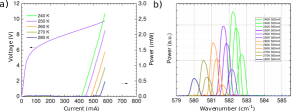
Figure 1: a) Optical output power and voltage versus drive current recorded for various QCL temperatures. b): Emission spectra, measured by a FTIR spectrometer for various QCL temperatures and drive currents.

h

Figure 2: Measured linear absorption spectrum of N₂O (red curve) realised at a pressure of $500$ Pa. The stick spectrum is taken from the NIST database and corresponds to transitions of various N₂O isotopologues, the main contributions are given by the N¹⁴N¹⁴O¹⁶ isotopologue (abundance 99%). The blue sticks Wells et al. (1985); Vanek et al. (1989); Maki and Wells (1992) are characterized by a better accuracy than the black sticksMaki and Wells (1991, 1992, 1998). The three main absorption lines belong to the P branch of the fundamental transitions of the v₂ bending mode (P8, P9 and P10 at $582.07$, $581.24$ and $580.4$ cm^-1 respectively), while other transitions correspond to hot bands of the same v₂ mode.

The active region of the QCL is formed from InAs/AlSb Baranov et al. (2016); Nguyen Van et al. (2019). The laser chip is mounted on a Peltier-cooled module. The laser spectra and output power are shown on Fig.1. Several milliwatts of optical power can be generated, over a frequency range of $\sim 3~{}\textrm{cm}^{-1}$ ($\sim 100$ GHz) by tuning the temperature and drive current. The QCL beam is collimated by a parabolic mirror mounted a few millimeters away from the laser chip.

We realized N₂O absorption spectroscopy over the full tuning range of the QCL. There has hardly been any previous laser spectroscopy of N₂O in this spectral region. The first laser spectroscopy of N₂O around $17\,\mu$m was performed in 1978 by Reisfeld and FlickerReisfeld and Flicker (1979) using a lead salt laser followed later on by the references Baldacchini et al. (1992, 1993). However, these works were hampered by the poor laser performance, such as a broad emission bandwidth and mode hopping. Lead salt lasers present the user with other significant problems, including spectral properties that vary after temperature cycling. QCLs offer a much more reliable and precise alternative as we demonstrate in this article.

In order to explore the full frequency range of the QCL, seven spectral measurements were made, each recorded with different laser operating conditions. For these measurements, the laser temperature set-point was varied from -28.5°C to -2.6°C; for each temperature the unmodulated laser drive current was set around $525$ mA. For each measurement the output frequency was scanned by applying a current ramp of amplitude $\sim\pm 0.5$ mA and period $100$ ms. In this way, N₂O absorption data were recorded in the range from 580 cm^-1 to 582.5 cm^-1. The absorption spectra were recorded with N₂O pressure of $500$ Pa in a $24$ cm long gas cell using a liquid nitrogen-cooled photoconductive HgCdTe (MCT) detector. For each measurement, reference measurements were made in order to allow transmission spectra to be calculated. The first reference measurement was performed with the laser blocked, which allowed the MCT dark signal to be recorded. The second reference measurement was performed with the laser unblocked, but with the gas cell evacuated, which allowed the transmission of the gas cell itself to be measured (including the effects of etalon fringing). With these reference measurements, transmission spectra were generated, with fringing effects largely removed. The frequency scale of each spectrum was calibrated using the NIST database Wavenumbers for Calibration of IR SpectrometersMaki and Wells (1991, 1992, 1998). For each spectrum around eight strong absorption features, covering the full frequency range of the spectrum, were selected for the calibration procedure. A Gaussian function was fitted to each of the selected features, in order to find the line centre in units of the scan data-point number. The known line centres from the NIST database (units of $\textrm{cm}^{-1}$) were then plotted against the uncalibrated line centres, and a third order polynomial function was fitted to the line centre data. The polynomial function was then used to calibrate the spectrum frequency scale. The spectra were recorded with sufficient overlap to allow them to be combined into one spectrum, shown in Fig. 2, where the three large amplitude features in this spectrum correspond to the lines in the P branch of the v₂ fundamental mode (the bending mode), and all other features correspond to hot bands of the same mode.

We also characterized the frequency noise properties of this $17$ $\mu$m QCL. As illustrated in Fig.3, the P9 absorption feature of the v₂ mode ($581.24$ cm^-1) was used as a frequency-to-amplitude converter Bartalini et al. (2010); Sow et al. (2014). The P9 line is measured for a N₂O pressure of $100$ Pa, resulting in a large absorption signal and limited collision-induced broadening. The lineshape is fitted to a Voigt profile. The frequency scale is calibrated using the Doppler width as a reference. A FWHM of $63$ MHz is obtained for the fitted Voigt profile. This is much larger than the linewidth at any time scale of the QCL, as will be shown after. This implies that the laser frequency noise is well within the linear response range of our molecular frequency-to-amplitude converter Kashanian et al. (2016). Once the line profile measured, the laser frequency is locked to the side of the P9 feature. The lock bandwidth was 1 Hz, chosen to stop slow drift of the laser frequency, but without suppressing higher frequency components. The amplitude noise generated by the molecular line frequency discriminator is measured with the MCT detector and processed by a Fast Fourier Transform (FFT) spectrum analyzer. The frequency-to-amplitude conversion coefficient is the derivative of the measured P9 rovibrational line profile shown in Fig.3 at the position where the laser line is parked Bartalini et al. (2010, 2011); Sow et al. (2014). For the following frequency noise measurements, the $17$ $\mu$m QCL is operated at a temperature of $258$ K and a current of $570$ mA.

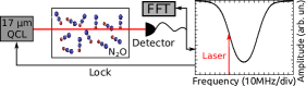
Figure 3: QCL frequency noise measurement setup. A $24$-cm long cell filled at a N₂O pressure $P=100$ Pa is used as a frequency-to-intensity converter. The QCL frequency is locked to the side of the N₂O P9 line ($581.24$ cm^-1) of the $v_{2}$ vibrational bending mode. The lock bandwidth was $1$ Hz to correct for slow frequency drifts without suppressing higher frequency components. Intensity fluctuations proportional to the laser frequency noise are measured with a liquid nitrogen-cooled photoconductive HgCdTe detector and processed by a Fast Fourier Transform (FFT) spectrum analyzer.

The frequency noise PSD of the QCL is shown in Fig.4, red curve. We also measured the contribution from the laser intensity noise (blue line in Fig.4), obtained with the laser tuned far from any molecular resonance, as well as the contribution from a home-made low-noise current source (black line in Fig.4) obtained by multiplying the driver’s current noise spectrum by the laser DC current-to-frequency response of $240$ MHz/mA Sow et al. (2014). This value is the local slope at $260$ K and $570$ mA of the measured QCL frequency shift versus driving current, obtained from the FTIR spectrum measurements (fig.1b). The intensity and driver’s contribution are negligibly small compared to the frequency noise, except at low frequencies ($<10$ Hz) at which the laser driver current noise will contribute to the laser frequency noise.

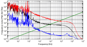
Figure 4: Frequency noise power spectral density (PSD) of the $17$ $\mu$m QCL (red line) and $\beta$-separation line (green line) to estimate the linewidth. The contributions of the laser intensity noise (blue line) and laser driver current noise (black line) are also shown for comparison. The laser intensity contribution has been recorded with the same QCL parameters (temperature, current) as in the frequency noise measurement. The optical power hitting the detector was attenuated to be equivalent to the case with molecular absorption.

At low frequencies ($\lesssim 100$ kHz) the QCL frequency noise (Fig.4 red) is dominated by usual $1/f$ noise . However, for frequencies greater than $100$ kHz, a noise plateau appears, as has been reported for other QCLs at shorter wavelengths Bartalini et al. (2010, 2011). This white noise level $N_{w}=30.4\times 10^{3}$ Hz²/Hz corresponds to an intrinsic Lorentzian FWHM linewidth of $\Delta\nu_{l}=\pi N_{w}=96$ kHz. For frequencies greater than $500$ kHz, the frequency noise PSD falls of rapidly due to the limited bandwidth of our photoconductive MCT detector. Following the theoretical work for a 3 level QCL described in reference Yamanishi et al. (2007), we calculated the expected FWHM intrinsic lorentzian linewidth of the $17$ $\mu$m laser $\Delta\nu_{l,th}$. The details of this calculation including a comparison with other QCLs are presented in the Supplementary Material. We find for this laser at the given operated conditions $\Delta\nu_{l,th}\simeq 400$ Hz. The measured noise plateau gives therefore an intrinsic linewidth two orders of magnitude larger than the theoretical calculation. We do not have an explanation for this discrepancy. Measured or inferred intrinsic linewidth for QCLs at $4.3$ and $10.6$ $\mu$m Bartalini et al. (2010, 2011); Sow et al. (2014) tend to agree with theoretical calculations, with reported values of the order of $100$ Hz.

Using the frequency noise PSD, one can also estimate the lineshape and FWHM linewidth of the QCL including the dominant $1/f$ noise below $100$ kHz. The FWHM linewidth can be calculated with a good approximation using the $\beta$-separation line method as described in reference Di Domenico et al. (2010). The $\beta$-separation line is shown in Fig.4 as a green line. Noise components at frequencies greater than the cutoff defined by the crossing point between the $\beta$-separation line and the frequency noise PSD ($f_{c}=60$ kHz) are discarded in the estimation of the laser linewidth. The estimated FWHM linewidth evolution with the integration time is shown in Fig.5, solid red line. We find $\Delta\nu=240$ kHz at $1$ s integration time. The $\beta$-separation linewidth is not reported for small integration time ($<100$ $\mu$s) approaching the cutoff ($1/f_{c}=16$ $\mu$s) as the approximation discards high frequency noise components and therefore fails in estimating correctly the linewidth in this case Di Domenico et al. (2010). To overcome the limitations of the $\beta$-separation line method we calculated the $17$ $\mu$m laser lineshape (Fig.5 inset) at various integration time from the frequency noise PSD following reference Elliott et al. (1982) and accounting for the integration time Bishof et al. (2013); Sow et al. (2014). For integration times larger than $1$ ms, the lineshape is approaching a Gaussian distribution due to the $1/f$ noise contribution (Fig.5 inset, blue and green lines). The corresponding FWHM linewidth are reported as square points on Fig.5, agreeing reasonably well with the $\beta$-separation line method. The former method under-estimates the linewidth by 10% for pure 1/f noise Di Domenico et al. (2010). A larger disagreement (20%) between the $\beta$-separation line method and the laser lineshape calculation is observed in our case owing to the contribution of the white noise plateau. The calculated FWHM linewidth decreases with decreasing integration time, reaches a minimum of $30$ kHz at $33$ $\mu$s integration. For smaller integration, the linewidth is limited by the measurement time and therefore increases.

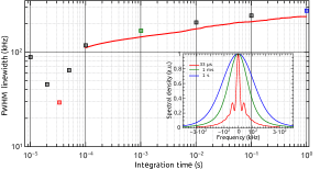
Figure 5: FWHM linewidth as a function of integration time calculated from the frequency noise PSD presented in Fig.4. Red line: $\beta$-separation line method, square points: FWHM linewidth inferred from a lineshape reconstruction. The inset shows the calculated QCL line shape for three integration times: $1$ s (blue), $1$ ms (green) and $33$ $\mu$s (red).

This new, narrow-linewidth laser offers new spectroscopic opportunities in the MIR, e.g. as the local oscillator of a heterodyne detector for astrophysical molecular detection at $17~{}\mu$m Bourdarot et al. (2020, 2021), or the manipulation of bismuth spin states in silicon for solid-state quantum technology and atomic clock applications Saeedi et al. (2015). One of our goal is to extend to longer wavelengths, at which IVR is reduced, the frequency metrology methods for frequency stabilisation recently demonstrated for QCLs at $10~{}\mu$m and below Bielsa et al. (2007); Sow et al. (2014); Hansen et al. (2015); Argence et al. (2015); Insero et al. (2017); Santagata et al. (2019). This opens perspectives for using increasingly complex polyatomic molecules to perform tests of fundamental physics, e.g. to measure the energy difference between enantiomers of a chiral molecule, a signature of weak-interactions-induced parity violation Cournol et al. (2019); Fiechter et al. (2022), and a sensitive probe of dark matter Gaul et al. (2020). Longer wavelength QCLs are also necessary to develop frequency standards in the mid-infrared based on ultra-cold diatomic molecules and the QCL used for the present study has been designed to coincide with the vibration at $17.2$ $\mu$m of CaF Kaledin et al. (1999), one of the few molecules that can be laser cooled down to the microkelvin range Truppe et al. (2017). A clock based on the fundamental vibrational transition of ultra-cold CaF molecules confined in an optical trap is currently under construction Barontini et al. (2022). It is expected to have a linewidth below 10 Hz, a stability of $2\times 10^{-15}$ at 1 s, and the potential to measure the stability of the electron-to-proton mass ratio to a fractional precision better than $10^{-17}$ per year.

In conclusion, we have performed absorption spectroscopy of N₂O to demonstrate the spectroscopic capabilities of a new QCL operating at $17$ $\mu$m . This laser operates in a spectral region that is poorly covered by existing lasers, and its development opens new opportunities in atmospheric sensing and chemical detection, as well as in precise spectroscopic tests of fundamental physics. We have used this spectroscopy to probe the frequency characteristics of the laser, measuring the laser linewidth, the value of which disagrees with theoretical understanding of the noise associated with QCLs. This characterization of the frequency noise is a first step towards a frequency stabilization of this source for subsequent precise spectroscopy in this long wavelength region.

See the supplementary material for details on the intrinsic linewidth calculation as well as a comparison with reported data for other QCLs. TEW acknowledges funding from the Royal Society International Exchanges Scheme (grant IES\R3\183175), the Imperial College European Partners Fund and the Université Sorbonne Paris Nord Visiting Fellow Fund.

Appendix A Supplementary material

	Reference Bartalini et al. (2010)	Reference Bartalini et al. (2011)	$17$ $\mu$m QCL
$\tau_{21}$ (s)	$0.25\times 10^{-12}$	$0.15\times 10^{-12}$	$0.073\times 10^{-12}$
$\tau_{31}$ (s)	$2\times 10^{-12}$	$1.79\times 10^{-12}$	$0.29\times 10^{-12}$
$\tau_{32}$ (s)	$3.4\times 10^{-12}$	unknown	$0.92\times 10^{-12}$
$\tau_{r}$ (s)	$7.5\times 10^{-9}$	$10\times 10^{-9}$	$52\times 10^{-9}$
$\tau_{t}$ (s)	$1.26\times 10^{-12}$	$1\times 10^{-12}$	$0.2\times 10^{-12}$
$\eta$	$0.7$	$0.7$	$0.9$
$\beta$	$9.5\times 10^{-5}$	$5\times 10^{-5}$	$7.2\times 10^{-4}$
$\gamma$ (Hz)	$1.2\times 10^{11}$	$1.2\times 10^{11}$	$3.1\times 10^{11}$
$\beta_{eff}$	$1.6\times 10^{-8}$	$5\times 10^{-9}$	$1.9\times 10^{-9}$
$\epsilon$	$0.25$	$0.2$	$0.3$
$I/I_{th}$	$1.54$	$1.15$	$1.2$
$\bm{\Delta\nu_{l,th}}$ (Hz)	$\mathbf{510}$	$\mathbf{340}$	$\mathbf{380}$

Table 1: Values of the parameters to calculate the intrinsic QCL linewidth given by eq.1, comparison between the $17$ $\mu$m QCLs and QCLs presented in references Bartalini et al. (2010, 2011). Reference Bartalini et al. (2010) and Bartalini et al. (2011) used DFB QCLs, a $4.33$ $\mu$m QCL cooled at liquid-nitrogen temperatures and a $4.36$ $\mu$m QCL working at room-temperature respectively.

Figure 6: Schematics of the quantum levels of a given potential well for a 3 level QCL. The radiative relaxation between level 3 and 2 producing photons is represented in red and characterized by a relaxation time $\tau_{r}$. The other relaxation paths described are non-radiative. The total relaxation time of level 3 is $\tau_{t}=(1/\tau_{r}+1/\tau_{32}+1/\tau_{31})^{-1}$.

In this supplementary material we describe the calculation of the theoretical intrinsic linewidth of the $17$ $\mu$m laser, following the work by Yamanishi et al. Yamanishi et al. (2007) for a 3 level QCL as depicted on Fig.6. The theoretical FWHM intrinsic linewidth $\Delta\nu_{l,th}$ of the $17$ $\mu$m laser is given by

$$\Delta\nu_{l,th}=\frac{\gamma\beta_{eff}}{4\pi(1-\epsilon)}\bigg{[}\frac{1}{I/I{th}-1}+\epsilon\bigg{]}(1+\alpha_{e}^{2}),$$ (1)

corresponding to equation (2) in reference Bartalini et al. (2010), which is equivalent to eq. (16a) in reference Yamanishi et al. (2007). $\epsilon=\frac{\tau_{21}\tau_{31}}{\eta\tau_{t}(\tau_{21}+\tau_{31})}$ is a parameter depending on the relaxation times of the various levels and on the injection efficiency $\eta$ of the charges in level 3. The Henry linewidth enhancement factor $\alpha_{e}$ is close to $0$ for QCLs Faist et al. (1994); Von Staden et al. (2006); Kumazaki et al. (2008). $I$ and $I_{th}$ correspond to the injected and lasing threshold current. $\gamma$ is the photon decay rate, $\beta_{eff}=\beta\tau_{r}/\tau_{t}$ the effective coupling of the spontaneous emission, the ratio of spontaneous emission rate coupled into the lasing mode $\beta\tau_{r}$ to the total relaxation rate of the upper level $\tau_{t}$. This number is typically small for QCLs due to very efficient nonradiative processes ($\tau_{r}\ll\tau_{t}$). This in terms explains the narrow intrinsic linewidth of QCLs due to a reduction of the noise associated to spontaneous emission. The order of magnitude of $\Delta\nu_{l,th}$ is mainly determined by the product $\gamma\beta_{eff}$.

The values of the various parameters in eq.1 are reported in table 1 for the $17$ $\mu$m laser as well as for the QCLs of references Bartalini et al. (2010, 2011) for comparison. Reference Bartalini et al. (2010) and Bartalini et al. (2011) used DFB QCLs, a $4.33$ $\mu$m QCL cooled at liquid-nitrogen temperatures and a $4.36$ $\mu$m QCL working at room-temperature respectively.

Following notations from Yamanishi et al Yamanishi et al. (2007), we give below the various physical quantities characterizing the $17$ $\mu$m QCL necessary to derive its intrinsic linewidth and parameters presented in table 1. The cavity of the $17$ $\mu$m QCL is single mode (TM₀₀). The waveguide core thickness is $t_{g}=5.2$ $\mu$m, the core width $w_{g}=14$ $\mu$m and the cavity length $L_{c}=3$ mm. The cavity mode effective refractive index is $n_{eff}=3.34$, the refractive index of the waveguide active material $n_{g}=3.38$, while the cladding and group indices are $n_{c}=3$ and $n_{gr}=3.77$ respectively. The optical confinement of the mode is such that $\Gamma_{Conf,y}=1$ and $\Gamma_{Conf,z}=0.64$. We find a z-oriented dipole moment of $|\langle\phi_{3}|z|\phi_{2}\rangle$ of $6.2$ nm. The overall cavity losses are expected to be $\alpha_{tot}=3500$ m^-1, which gives a photon decay rate of $\gamma=0.3$ THz. The guided spontaneous relaxation is calculated to be $\tau_{rg}=790$ ns (eq. (A10a) in Yamanishi et al. (2007)), while the spontaneous relaxation partly coupled to the free-space continuum mode is $\tau_{rfp}=92$ ns (eq. (A6b) in Yamanishi et al. (2007)) and thus a total radiative lifetime $\tau_{r}=82$ ns (eq. (A11) in Yamanishi et al. (2007)). With this, we calculate a coupling efficiency of spontaneous emission to the guide of $\beta_{guide}=0.11$ (eq. (A12) in Yamanishi et al. (2007)), and a coupling efficiency of spontaneous emission to a single longitudinal mode of $\beta_{l}=0.007$ (eq. (A13a) in Yamanishi et al. (2007)), wich gives a coupling efficiency of spontaneous emission into a single lasing mode $\beta=\beta_{l}\times\beta_{guide}=7\times 10^{-4}$. The effective coupling efficiency is then $\beta_{eff}=1.9\times 10^{-9}$. The injection efficiency $\eta$ of the charges in level 3 is measured to be 0.9. As for the experimental parameters, a current $I=570$ mA was fed to the $17$ $\mu$m QCL operating at a temperature $T=258$ K, with a corresponding lasing threshold of $I_{th}=480$ mA. Finally, a theoretical intrinsic linewidth $\Delta\nu_{l,th}$ of $380$ Hz is calculated, comparable to the two cases reported in the literature.

References

- Faist et al. (1994) J. Faist, F. Capasso, D. L. Sivco, C. Sirtori, A. L. Hutchinson, and A. Y. Cho, Science 264, 553 (1994).
- Corrigan et al. (2009) P. Corrigan, R. Martini, E. A. Whittaker, and C. Bethea, Optics Express 17, 4355 (2009).
- Liu et al. (2019) J. J. Liu, B. L. Stann, K. K. Klett, P. S. Cho, and P. M. Pellegrino, SPIE Conference Proceedings 11133, 1113302 (2019), publisher: SPIE.
- Corrias et al. (2022) N. Corrias, T. Gabbrielli, P. De Natale, L. Consolino, and F. Cappelli, Optics Express 30, 10217 (2022).
- Nikodem and Wysocki (2012) M. Nikodem and G. Wysocki, Sensors 12, 16466 (2012).
- Daghestani et al. (2014) N. S. Daghestani, R. Brownsword, and D. Weidmann, Optics Express 22, A1731 (2014).
- Martín-Mateos et al. (2017) P. Martín-Mateos, J. Hayden, P. Acedo, and B. Lendl, Analytical Chemistry 89, 5916 (2017).
- Robinson et al. (2021) I. Robinson, H. L. Butcher, N. A. Macleod, and D. Weidmann, Optics Express 29, 2299 (2021).
- Galli et al. (2016) I. Galli, S. Bartalini, R. Ballerini, M. Barucci, P. Cancio, M. D. Pas, G. Giusfredi, D. Mazzotti, N. Akikusa, and P. D. Natale, Optica 3, 385 (2016), publisher: Optica Publishing Group.
- Bielsa et al. (2008) F. Bielsa, K. Djerroud, A. Goncharov, A. Douillet, T. Valenzuela, C. Daussy, L. Hilico, and A. Amy-Klein, Journal of Molecular Spectroscopy 247, 41 (2008).
- Asselin et al. (2017) P. Asselin, Y. Berger, T. R. Huet, L. Margulès, R. Motiyenko, R. J. Hendricks, M. R. Tarbutt, S. K. Tokunaga, and B. Darquié, Physical Chemistry Chemical Physics 19, 4576 (2017), publisher: The Royal Society of Chemistry.
- Borri et al. (2019) S. Borri, G. Insero, G. Santambrogio, D. Mazzotti, F. Cappelli, I. Galli, G. Galzerano, M. Marangoni, P. Laporta, V. Di Sarno, et al., Applied Physics B 125, 1 (2019).
- D’Ambrosio et al. (2019) D. D’Ambrosio, S. Borri, M. Verde, A. Borgognoni, G. Insero, P. De Natale, and G. Santambrogio, Physical Chemistry Chemical Physics 21, 24506 (2019).
- Bielsa et al. (2007) F. Bielsa, A. Douillet, T. Valenzuela, J.-P. Karr, and L. Hilico, Opt. Lett. 32, 1641 (2007).
- Sow et al. (2014) P. L. T. Sow, S. Mejri, S. K. Tokunaga, O. Lopez, A. Goncharov, B. Argence, C. Chardonnet, A. Amy-Klein, C. Daussy, and B. Darquié, Applied Physics Letters 104, 264101 (2014).
- Hansen et al. (2015) M. G. Hansen, E. Magoulakis, Q.-F. Chen, I. Ernsting, and S. Schiller, Optics Letters 40, 2289 (2015), publisher: OSA.
- Argence et al. (2015) B. Argence, B. Chanteau, O. Lopez, D. Nicolodi, M. Abgrall, C. Chardonnet, C. Daussy, B. Darquié, Y. Le Coq, and A. Amy-Klein, Nature Photonics 9, 456 (2015).
- Insero et al. (2017) G. Insero, S. Borri, D. Calonico, P. C. Pastor, C. Clivati, D. D’ambrosio, P. De Natale, M. Inguscio, F. Levi, and G. Santambrogio, Scientific reports 7, 1 (2017).
- Santagata et al. (2019) R. Santagata, D. Tran, B. Argence, O. Lopez, S. Tokunaga, F. Wiotte, H. Mouhamad, A. Goncharov, M. Abgrall, Y. Le Coq, et al., Optica 6, 411 (2019).
- Mejri et al. (2015) S. Mejri, P. L. T. Sow, O. Kozlova, C. Ayari, S. K. Tokunaga, C. Chardonnet, S. Briaudeau, B. Darquié, F. Rohart, and C. Daussy, Metrologia 52, S314 (2015), iSBN: 0026-1394.
- Cournol et al. (2019) A. Cournol, M. Manceau, M. Pierens, L. Lecordier, D. Tran, R. Santagata, B. Argence, A. Goncharov, O. Lopez, M. Abgrall, et al., Quantum Electronics 49, 288 (2019).
- Lukusa Mudiayi et al. (2021) J. Lukusa Mudiayi, I. Maurin, T. Mashimo, J. de Aquino Carvalho, D. Bloch, S. Tokunaga, B. Darquié, and A. Laliotis, Physical Review Letters 127, 043201 (2021), publisher: American Physical Society.
- Petrov (2012) V. Petrov, Optical Materials 34, 536 (2012).
- Schliesser et al. (2012) A. Schliesser, N. Picqué, and T. W. Hänsch, Nature photonics 6, 440 (2012).
- Leindecker et al. (2011) N. Leindecker, A. Marandi, R. L. Byer, and K. L. Vodopyanov, Optics express 19, 6296 (2011).
- Sotor et al. (2018) J. Sotor, T. Martynkien, P. G. Schunemann, P. Mergo, L. Rutkowski, and G. Soboń, Optics express 26, 11756 (2018).
- Lamperti et al. (2020) M. Lamperti, R. Gotti, D. Gatti, M. K. Shakfa, E. Cané, F. Tamassia, P. Schunemann, P. Laporta, A. Farooq, and M. Marangoni, Communications Physics 3, 175 (2020).
- Cathabard et al. (2010) O. Cathabard, R. Teissier, J. Devenson, J. C. Moreno, and A. N. Baranov, Applied Physics Letters 96, 141110 (2010), publisher: American Institute of Physics.
- Ohtani et al. (2016) K. Ohtani, M. Beck, M. J. Süess, J. Faist, A. M. Andrews, T. Zederbauer, H. Detz, W. Schrenk, and G. Strasser, ACS Photonics 3, 2280 (2016), publisher: American Chemical Society.
- Jackson and Jain (2020) S. D. Jackson and R. Jain, Optics Express 28, 30964 (2020).
- Vasilyev et al. (2016) S. Vasilyev, I. Moskalev, M. Mirov, V. Smolsky, S. Mirov, and V. Gapontsev, Laser Technik Journal 13, 24 (2016).
- Faist et al. (1997) J. Faist, C. Gmachl, F. Capasso, C. Sirtori, D. L. Sivco, J. N. Baillargeon, and A. Y. Cho, Applied Physics Letters 70, 2670 (1997).
- Pirali et al. (2006) O. Pirali, N.-T. Van-Oanh, P. Parneix, M. Vervloet, and P. Bréchignac, Physical Chemistry Chemical Physics 8, 3707 (2006).
- Huang et al. (2011) X. Huang, W. O. Charles, and C. Gmachl, Optics Express 19, 8297 (2011), publisher: Optica Publishing Group.
- Fuchs et al. (2011) P. Fuchs, J. Semmel, J. Friedl, S. Höfling, J. Koeth, L. Worschech, and A. Forchel, Applied Physics Letters 98, 211118 (2011).
- Elkhazraji et al. (2023a) A. Elkhazraji, M. K. Shakfa, M. Lamperti, K. Hakimov, K. Djebbi, R. Gotti, D. Gatti, M. Marangoni, and A. Farooq, Optics Express 31, 4164 (2023a).
- Elkhazraji et al. (2023b) A. Elkhazraji, M. Adil, M. Mhanna, N. Abualsaud, A. A. Alsulami, M. K. Shakfa, M. Marangoni, B. Giri, and A. Farooq, Proceedings of the Combustion Institute 39, 1485 (2023b).
- Bourdarot et al. (2020) G. Bourdarot, H. G. de Chatellus, and J.-P. Berger, Astronomy & Astrophysics 639, A53 (2020).
- Bourdarot et al. (2021) G. Bourdarot, J.-P. Berger, and H. G. de Chatellus, JOSA B 38, 3105 (2021).
- Barontini et al. (2022) G. Barontini, L. Blackburn, V. Boyer, F. Butuc-Mayer, X. Calmet, J. R. Crespo López-Urrutia, E. A. Curtis, B. Darquié, J. Dunningham, N. J. Fitch, E. M. Forgan, K. Georgiou, P. Gill, R. M. Godun, J. Goldwin, V. Guarrera, A. C. Harwood, I. R. Hill, R. J. Hendricks, M. Jeong, M. Y. H. Johnson, M. Keller, L. P. Kozhiparambil Sajith, F. Kuipers, H. S. Margolis, C. Mayo, P. Newman, A. O. Parsons, L. Prokhorov, B. I. Robertson, J. Rodewald, M. S. Safronova, B. E. Sauer, M. Schioppo, N. Sherrill, Y. V. Stadnik, K. Szymaniec, M. R. Tarbutt, R. C. Thompson, A. Tofful, J. Tunesi, A. Vecchio, Y. Wang, and S. Worm, EPJ Quantum Technology 9, 1 (2022).
- Nesbitt and Field (1996) D. J. Nesbitt and R. W. Field, The Journal of Physical Chemistry 100, 12735 (1996).
- Brumfield et al. (2012) B. E. Brumfield, J. T. Stewart, and B. J. McCall, The Journal of Physical Chemistry Letters 3, 1985 (2012).
- Spaun et al. (2016) B. Spaun, P. B. Changala, D. Patterson, B. J. Bjork, O. H. Heckl, J. M. Doyle, and J. Ye, Nature 533, 517 (2016).
- Nguyen Van et al. (2019) H. Nguyen Van, Z. Loghmari, H. Philip, M. Bahriz, A. N. Baranov, and R. Teissier, Photonics 6 (2019), 10.3390/photonics6010031.
- Wells et al. (1985) J. S. Wells, A. Hinz, and A. G. Maki, Journal of Molecular Spectroscopy 114, 84 (1985).
- Vanek et al. (1989) M. D. Vanek, M. Schneider, J. S. Wells, and A. G. Maki, Journal of Molecular Spectroscopy 134, 154 (1989).
- Maki and Wells (1992) A. G. Maki and J. S. Wells, Journal of Research of the National Institute of Standards and Technology 97, 409 (1992).
- Maki and Wells (1991) A. G. Maki and J. S. Wells, Wavenumber Calibration Tables From Heterodyne Frequency Measurements (NIST Special Publication 821, 1991).
- Maki and Wells (1998) A. G. Maki and J. S. Wells, “Wavenumbers for calibration of IR spectrometers,” Physical Measurement Laboratory, NIST, https://www.nist.gov/pml/wavenumbers-calibration-ir-spectrometers (1998).
- Baranov et al. (2016) A. N. Baranov, M. Bahriz, and R. Teissier, Opt. Express 24, 18799 (2016).
- Reisfeld and Flicker (1979) M. J. Reisfeld and H. Flicker, Appl. Opt. 18, 1136 (1979).
- Baldacchini et al. (1992) G. Baldacchini, P. K. Chakraborti, and F. D’Amato, Applied Physics B 55, 92 (1992).
- Baldacchini et al. (1993) G. Baldacchini, P. Chakraborti, and F. D’Amato, Journal of Quantitative Spectroscopy and Radiative Transfer 49, 439 (1993).
- Bartalini et al. (2010) S. Bartalini, S. Borri, P. Cancio, A. Castrillo, I. Galli, G. Giusfredi, D. Mazzotti, L. Gianfrani, and P. De Natale, Physical review letters 104, 083904 (2010).
- Kashanian et al. (2016) S. V. Kashanian, A. Eloy, W. Guerin, M. Lintz, M. Fouché, and R. Kaiser, Physical Review A 94, 043622 (2016).
- Bartalini et al. (2011) S. Bartalini, S. Borri, I. Galli, G. Giusfredi, D. Mazzotti, T. Edamura, N. Akikusa, M. Yamanishi, and P. De Natale, Optics express 19, 17996 (2011).
- Yamanishi et al. (2007) M. Yamanishi, T. Edamura, K. Fujita, N. Akikusa, and H. Kan, IEEE Journal of Quantum Electronics 44, 12 (2007).
- Di Domenico et al. (2010) G. Di Domenico, S. Schilt, and P. Thomann, Applied optics 49, 4801 (2010).
- Elliott et al. (1982) D. Elliott, R. Roy, and S. Smith, Physical Review A 26, 12 (1982).
- Bishof et al. (2013) M. Bishof, X. Zhang, M. J. Martin, and J. Ye, Physical Review Letters 111, 093604 (2013).
- Saeedi et al. (2015) K. Saeedi, M. Szech, P. Dluhy, J. Z. Salvail, K. J. Morse, H. Riemann, N. V. Abrosimov, N. Nötzel, K. L. Litvinenko, B. N. Murdin, and M. L. W. Thewalt, Scientific Reports 5, 10493 (2015), number: 1 Publisher: Nature Publishing Group.
- Fiechter et al. (2022) M. R. Fiechter, P. A. B. Haase, N. Saleh, P. Soulard, B. Tremblay, R. W. A. Havenith, R. G. E. Timmermans, P. Schwerdtfeger, J. Crassous, B. Darquié, L. F. Pašteka, and A. Borschevsky, “Towards detection of the molecular parity violation in chiral Ru(acac)$_3$ and Os(acac)$_3$,” (2022), arXiv:2111.05036 [physics].
- Gaul et al. (2020) K. Gaul, M. G. Kozlov, T. A. Isaev, and R. Berger, Physical Review Letters 125, 123004 (2020), publisher: American Physical Society.
- Kaledin et al. (1999) L. A. Kaledin, J. C. Bloch, M. C. McCarthy, and R. W. Field, Journal of Molecular Spectroscopy 197, 289 (1999).
- Truppe et al. (2017) S. Truppe, H. Williams, M. Hambach, L. Caldwell, N. Fitch, E. Hinds, B. Sauer, and M. Tarbutt, Nature Physics 13, 1173 (2017).
- Von Staden et al. (2006) J. Von Staden, T. Gensty, W. Elsäßer, G. Giuliani, and C. Mann, Optics letters 31, 2574 (2006).
- Kumazaki et al. (2008) N. Kumazaki, Y. Takagi, M. Ishihara, K. Kasahara, A. Sugiyama, N. Akikusa, and T. Edamura, Applied Physics Letters 92, 121104 (2008).