DyExplainer: Explainable Dynamic Graph Neural Networks

Abstract.

Graph Neural Networks (GNNs) resurge as a trending research subject owing to their impressive ability to capture representations from graph-structured data. However, the black-box nature of GNNs presents a significant challenge in terms of comprehending and trusting these models, thereby limiting their practical applications in mission-critical scenarios. Although there has been substantial progress in the field of explaining GNNs in recent years, the majority of these studies are centered on static graphs, leaving the explanation of dynamic GNNs largely unexplored. Dynamic GNNs, with their ever-evolving graph structures, pose a unique challenge and require additional efforts to effectively capture temporal dependencies and structural relationships. To address this challenge, we present DyExplainer, a novel approach to explaining dynamic GNNs on the fly. DyExplainer trains a dynamic GNN backbone to extract representations of the graph at each snapshot, while simultaneously exploring structural relationships and temporal dependencies through a sparse attention technique. To preserve the desired properties of the explanation, such as structural consistency and temporal continuity, we augment our approach with contrastive learning techniques to provide priori-guided regularization. To model longer-term temporal dependencies, we develop a buffer-based live-updating scheme for training. The results of our extensive experiments on various datasets demonstrate the superiority of DyExplainer, not only providing faithful explainability of the model predictions but also significantly improving the model prediction accuracy, as evidenced in the link prediction task.

1. Introduction

The advent of Graph Neural Networks (GNNs) has caused a veritable revolution in the field, and has been embraced with great enthusiasm due to their demonstrated efficacy in a variety of applications, ranging from node classification (Kipf and Welling, 2016) and link prediction (Zhang and Chen, 2018), to graph clustering (Liu et al., 2023) and recommender systems (Wu et al., 2022). However, these models are usually treated as black boxes, and their predictions lack understanding and explanations, thus preventing them to produce reliable solutions. Therefore, the study of the explainability of GNNs is in need. Recent research on GNN explainability mainly focuses on explaining the model predictions. However, the labyrinthine nature of GNNs has often resulted in their predictions being shrouded in mystery and lacking transparency. Consequently, the trustworthiness of their solutions is frequently called into question. To rectify this, the exploration and understanding of the explainability of GNNs have become imperative. The current research landscape in this arena primarily centers on demystifying the underlying mechanisms of GNN predictions, utilizing methods such as gradient-based techniques (Baldassarre and Azizpour, 2019; Pope et al., 2019), mask-based approaches (Ying et al., 2019; Luo et al., 2020; Yuan et al., 2021), and surrogate models (Vu and Thai, 2020) to shed light on the reasoning (Liang et al., 2022) behind them. These techniques endeavor to bring greater transparency to the predictions of GNNs and to provide a deeper insight into the thought process of the model.

The advancement in explainability in static GNNs has been substantial, yet the same cannot be said for dynamic GNNs. Despite this, dynamic GNNs have gained widespread use in real-world applications, as they are capable of handling graphs that change over time. Elevating the level of explainability in dynamic GNNs is of utmost importance as it can foster greater human trust in the model’s predictions. However, the dynamic and evolving nature of graphs presents several challenges. Firstly, learning in dynamic graphs involves taking into consideration not only the topology and node attributes at each time point but also the temporal dynamics, making it a formidable task to present explanations in a manner that is easily understood by humans. Secondly, the consecutive order of dynamic graphs imposes unique constraints on the continuity of explanations. Lastly, the underlying patterns in dynamic graphs may also evolve with changes in node features and topologies, making it a challenge to find a balance between the continuity and evolution of explanations.

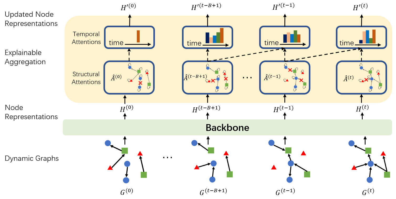
Figure 1. DyExplainer for dynamic graphs. ${\bm{H}}^{(t)}$ is the node representation for snapshot $G^{(t)}$ after backbone module. ${\bm{H}}^{\prime(t)}$ is the updated node representation after explainable module. $\widehat{{\bm{A}}}^{(t)}$ is the structural attention for snapshot $G^{(t)}$.

To handle these challenges, in this paper, we propose DyExplainer, a dynamic explainable mechanism for dynamically interpreting GNNs. DyExplainer constitutes a high-level, generalizable explainer that imparts insightful and comprehensible explanations through the utilization of graph patterns, thereby providing a deeper understanding of predictions made by diverse dynamic GNNs. The proposed approach incorporates pooling operations (Ying et al., 2018; Ma et al., 2019) on nodes, thereby yielding graph-level embeddings that are encoder-agnostic and afford a remarkable degree of flexibility to a broad spectrum of dynamic encoders serving as the backbone. Furthermore, the introduction of the explainer module into the encoder incurs only a minimal overhead, making it highly efficient for large-scale backbone networks. Specifically, DyExplainer trains a dynamic GNN model to produce node embeddings at each snapshot, where the explainer module comprises two attention components: structural attention and temporal attention. The former leverages the pivotal relationships between nodes within the graph at each snapshot to inform the node representations, while the latter accounts for the temporal dependencies between representations generated by long-term snapshots. Despite the proliferation of dynamic GNNs (You et al., 2022; Rossi et al., 2020), most of these approaches deduce the representation at each snapshot $t$ solely based on the embedding at the previous snapshot $(t-1)$, thereby making it challenging to fully comprehend the intricate, long-term temporal dependencies between snapshots in real-world applications. For instance, social network connections between individuals, groups, and communities may be subject to change over time, influenced by a multitude of factors, such as geographical distance, personal life stage, and evolving interests. To encompass longer-term temporal dependencies, we have devised a buffer-based, live-updating scheme with temporal attention. Specifically, the temporal attention aggregates the node embeddings from the preceding $B$ snapshots stored in a buffer. In this regard, prior works on dynamic GNNs are reduced to a special case of the DyExplainer, where $B=1$. The proposed framework constitutes a generalization that encompasses all recent graph learning methods for dynamic graphs. For example, by relinquishing explainability and incorporating the Markov chain property for temporal evolution, our framework degenerates to ROLAND (You et al., 2022). Additionally, by restricting temporal aggregations to only the final layer, our framework degenerates to a common approach in which a sequence model, such as GRU (Cho et al., 2014), is placed on top of GNNs (Peng et al., 2020; Wang et al., 2020; Yu et al., 2017).

The dual sparse attention components of DyExplainer serve a trifold function. Firstly, they impart incisive explanations for the model’s predictions in downstream tasks. Secondly, they serve as a sparse regularizer, enhancing the learning process. As research in the field of ranshomon set theory (Xin et al., 2022; Rudin et al., 2022) demonstrates, sparse and interpretable models possess a higher degree of robustness and better generalization performance, as outlined in Sec. 4.3. Lastly, the attention components allow for the augmentation of the approach with priori-guided regularization, preserving the desirable properties of the explanation, such as structural consistency and temporal continuity. Structural consistency pertains to the consistency of node embeddings between connected nodes in a single snapshot, while temporal continuity enforces smoothness constraints on the temporal attention between closely spaced snapshots, guided by pre-established human priors. To achieve more lucid explanations, we employ the use of contrastive learning techniques, treating connected pairs as positive examples and unconnected pairs as negative examples for consistency regularization, and recent snapshots as positive examples and distant historical snapshots as negative examples for continuity regularization. Overall, our contributions are summarized as follows:

• We put forward the problem of explainable dynamic GNNs and propose a general DyExplainer to tackle it. As far as we know, it is the first work solving this problem.

• DyExplainer seamlessly integrates the modeling of both structural relationships and long-term dependencies via sparse attentions. As a result, it is capable of providing real-time explanations for both the structural and temporal factors that influence the model’s predictions. This innovative explaining module has been designed to be encoder-agnostic, thereby affording flexibility to a range of dynamic GNN backbones. Its implementation requires minimal overhead, as it only entails adding a lightweight parameterization to the encoder for its explanation modules. This makes DyExplainer highly efficient even for large backbone networks.

• We propose two contrastive regularizations to provide consistency and continuity explanations. Our approach to augmenting desired properties in the explanation is a fresh contribution to the field and may be of independent interest.

• Extensive experiments on various datasets demonstrate the superiority of DyExplainer, not only providing faithful explainability of the model predictions but also significantly improving the model prediction accuracy, as evidenced in the link prediction task.

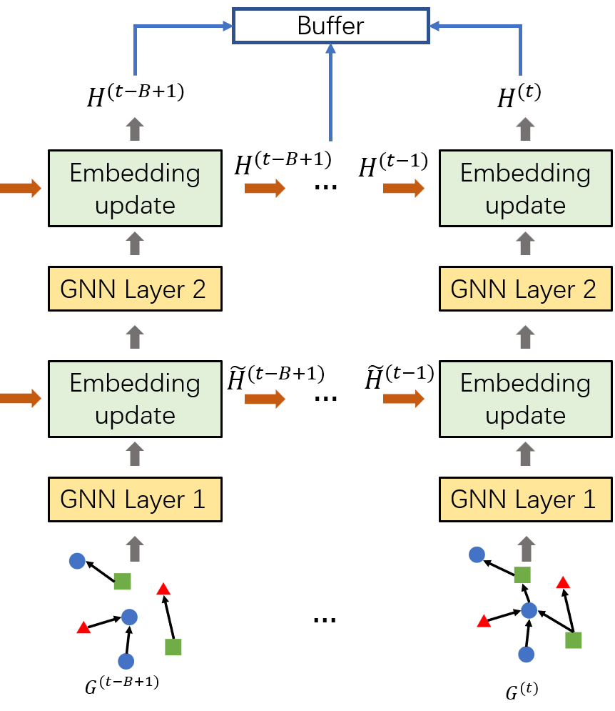
Figure 2. Backbone encoder architecture.

2. Problem Definition

We formulate a dynamic graph as a series of $T$ attributed graphs as ${\mathcal{G}}=(G^{(1)},...,G^{(T)})$, where each graph $G^{(t)}=({\mathcal{V}},{\mathcal{E}}^{(t)},{\bm{X}}^{(t)})$ is a snapshot at time step $t$. ${\mathcal{V}}=\{v_{1},v2,...v_{N}\}$ is the set of $N$ nodes shared by all snapshots and ${\mathcal{E}}^{(t)}\in{\mathcal{V}}\times{\mathcal{V}}$ is the set of edges of a graph $G^{(t)}$. ${\bm{X}}^{(t)}\in{\mathbb{R}}^{N\times D}$ is the node feature matrix at snapshot $t$, where $D$ is the number of dimensions of node features. The topology and node features of each snapshot are dynamically changing over time. We aim to learn an explainable dynamic GNN model $f$ from the long-term snapshots defined as:

(1) $$\widehat{{\bm{A}}}^{(t-B+1)},...,\widehat{{\bm{A}}}^{(t)},{\bm{H}}^{\prime(t+1)}\leftarrow f\left(G^{(t-B+1)},...,G^{(t)}\right),$$

where $\widehat{{\bm{A}}}^{(t-B+1)},...,\widehat{{\bm{A}}}^{(t)}$ are explanations we are interested and ${\bm{H}}^{\prime(t+1)}$ is the future node representation predicted for the downstream tasks. In our study, we examine its application for link prediction. It’s worth noting that our framework can also easily support other downstream tasks.

3. Method

3.1. Encoder Backbone

There are different approaches to designing dynamic GNNs. As a plug-and-use framework, the proposed DyExplainer is flexible to the choice of dynamic GNNs as the backbone. In this work, we adopt a state-of-the-art method ROLAND (You et al., 2022) as the backbone due to its powerful expressiveness and impressive empirical performances in real-life datasets. Specifically, it hierarchically updates the node embedding to obtain the ${\bm{H}}^{(t)}$ at snapshot $t$. With ROLAND as the backbone, the architecture of the encoder is shown in Figure 2. We put the node embedding inferred by the backbone to a buffer of size $B$ for the learning of our explainer module. Formally, we denote the node embeddings in the buffer as $\{{\bm{H}}^{(t-B+1)},...,{\bm{H}}^{(t)}\}$.

3.2. Explainable Aggregations

The node embedding at snapshot $t$ is denoted by ${\bm{H}}^{(t)}=\{{\bm{h}}_{1},...,{\bm{h}}_{N}\}$, ${\bm{h}}_{i}\in{\mathbb{R}}^{F}$, where $N$ is the number of nodes, and $F$ is the feature dimension of the node embedding.

3.2.1. Structural Aggregation

On dynamic graphs, each snapshot has its unique topology information. An effective explanation, therefore, should highlight the crucial structural components at a given snapshot that significantly contribute to the model’s prediction. To this end, inspired by the idea in (Veličković et al., 2017), we propose structural attention to aggregate the weighted neighborhoods at each time step. Formally, we have

(2) $$\omega^{(s,t)}_{ij}=\text{LeakyReLU}\Big{(}{\bm{a}}^{(s)T}\Big{[}{\bm{W}}^{(s)}{\bm{h}}^{(t)}_{i}||{\bm{W}}^{(s)}{\bm{h}}^{(t)}_{j}\Big{]}\Big{)},$$

(3) $$\widehat{{\bm{A}}}^{(t)}_{ij}=\mathrm{softmax}_{j}\Big{(}\omega^{(s,t)}_{ij}\Big{)}=\frac{\exp{\Big{(}\omega^{(s,t)}_{ij}}\Big{)}}{\sum_{k\in{\mathcal{N}}^{(t)}_{i}}\exp{\Big{(}\omega^{(s,t)}_{ik}\Big{)}}},$$

where $\widehat{{\bm{A}}}^{(t)}$ is the structural attention at time step $t$, ${\bm{W}}^{(s)}$ is a weight matrix in a shared linear transformation, ${\bm{a}}^{(s)}$ is the weight vector in the single-layer network, $\mathcal{N}^{(t)}_{i}$ is the set of neighbors of node $i$ at time step $t$, and $||$ indicates the concatenation operation.

However, the utilization of weights in traditional attention models may pose a challenge in complex dynamic graph environments, particularly with regard to explanation. Explanations in these settings are often derived by imposing a threshold and disregarding insignificant attention weights. This approach, however, fails to account for the cumulative impact of numerous small but non-zero weights, which can be substantial. Moreover, the non-exclusivity of attention weights raises questions about their accuracy in reflecting the true underlying importance (Veličković et al., 2017). To address this issue and equip structural attention with better explainability, we design a hard attention mechanism to alleviate the effects of small attention coefficients. The basic idea uses a prior work on differentiable sampling (Maddison et al., 2016; Jang et al., 2016), which states that the random variable

(4) $$e=\sigma\bigg{(}\Big{(}\log\epsilon-\log\big{(}1-\epsilon\big{)}+\omega\Big{)}/\tau\bigg{)}\quad\text{where}\quad\epsilon\sim\text{Uniform}\big{(}0,1\big{)},$$

where $\sigma(\cdot)$ is the sigmoid function and $\tau$ is the temperature controlling the approximation. Equation 4 follows a distribution that converges to a Bernoulli distribution with success probability $p=(1+e^{-\omega})^{-1}$ as $\tau>0$ tends to zero. Hence, if we parameterize $\omega$ and specify that the presence of an edge between a pair of nodes has probability $p$, then using $e$ computed from equation 4 to fill the corresponding entry of $\widehat{{\bm{A}}}$ will produce a matrix $\widehat{{\bm{A}}}$ that is close to binary. We use this matrix as the hard attention with the hope of obtaining a better explanation due to the dropping of small attention weights. Moreover, because equation 4 is differentiable with respect to $\omega$, we can train the parameters of $\omega$ like in a usual gradient-based training. In the structural attention, we have the parameterized $\omega^{(s,t)}_{ij}$ in Equation 2, thus we get

$$\widetilde{e}_{ij}^{(s,t)}=\sigma\bigg{(}\Big{(}\log\epsilon-\log\big{(}1-\epsilon\big{)}+\omega_{ij}^{(s,t)}\Big{)}/\tau\bigg{)}\quad\text{where}\quad\epsilon\sim\text{Uniform}\big{(}0,1\big{)},$$

which returns an approximate Bernoulli sample for the edge $(i,j)$. When $\tau$ is not sufficiently close to zero, this sample may not be close enough to binary, and in particular, it is strictly nonzero. The rationality of such an approximation is that with temperature $\tau>0$, the gradient $\frac{\partial\widetilde{e}_{ij}^{(s,t)}}{\partial\omega_{ij}^{(s,t)}}$ is well-defined. The output of the binary concrete distribution is in the range of (0,1). To further alleviate the effects of small values by encouraging them to be exactly zero, we propose a “stretching and clipping” technique in the hard attention mechanism. To explicitly zero out an edge, we follow (Louizos et al., 2017) and introduce two parameters, $\gamma<0$ and $\xi>1$, to remove small values of $\widetilde{e}_{ij}^{(s,t)}$given by

$$\widehat{{\bm{A}}}_{ij}^{(t)}=\min\Big{(}1,\max\big{(}e_{ij}^{(s,t)},0\big{)}\Big{)}\quad\text{where}\quad e_{ij}^{(s,t)}=\widetilde{e}_{ij}^{(s,t)}(\xi-\gamma)+\gamma.$$

The structural attention $\widehat{{\bm{A}}}^{(t)}$ does not insert new edges to the graph (i.e., when $(i,j)\notin{\mathcal{E}}^{(t)}$, $\widehat{{\bm{A}}}_{ij}^{(t)}=0$), but only removes (denoises) some edges $(i,j)$ originally in ${\mathcal{E}}^{(t)}$. Then, we obtain the node embedding $\widetilde{{\bm{H}}}^{(t)}\in{\mathbb{R}}^{N\times F^{\prime}}$ at the time step $t$ after the structural aggregation with each row given by

(5) $$\widetilde{{\bm{h}}}^{(t)}_{i}=\sigma\Big{(}\sum_{j\in{\mathcal{N}}_{i}^{(t)}}\widehat{{\bm{A}}}_{ij}^{(t)}{\bm{W}}^{(s)}{\bm{h}}_{j}^{(t)}\Big{)}.$$

3.2.2. Temporal Aggregation

In light of the dynamic and evolving nature of node features and inter-node relationships over time, temporal dependency holds paramount importance in the modeling of dynamic graphs. Existing methods either adopt RNN architectures, such as GRU (Cho et al., 2014) and LSTM (Hochreiter and Schmidhuber, 1997) or assume the Markow chain property (You et al., 2022) to capture the temporal dependencies in dynamic graphs. As shown in (Vaswani et al., 2017), despite their utility, these methods are insufficient in capturing long-range dependencies, thereby hindering their ability to generalize and model previously unseen graphs. To overcome this limitation, we propose a solution that leverages an attention-based temporal aggregation mechanism to adaptively integrate node embeddings from distant snapshots. This is achieved through the utilization of a buffer-dependent temporal mask, which serves as a temporal topology to guide the aggregation process.

In Equation 5, the structural attention provides the node embedding $\widetilde{{\bm{H}}}^{(t)}\in{\mathbb{R}}^{N\times F^{\prime}}$ for each snapshot $t$. Therefore, we have a set of node embedding $\{\widetilde{{\bm{H}}}^{(t-B+1)},...,\widetilde{{\bm{H}}}^{(t)}\}$. Concatenating them to a 3-dimensional tensor and take transpose, for each node $i$, we have a buffer-dependent node embedding $\widehat{{\bm{H}}}^{(i)}\in{\mathbb{R}}^{B\times F^{\prime}}$, $\widehat{{\bm{H}}}^{(i)}=\{\widehat{{\bm{h}}}_{t-B+1},...,\widehat{{\bm{h}}}_{t}\}$, $\widehat{{\bm{h}}}_{t}\in{\mathbb{R}}^{F^{\prime}}$. We propose the temporal attention given by

(6) $$\omega^{(i)}_{t_{k},t_{j}}=\text{LeakyReLU}\Big{(}{\bm{a}}^{T}\Big{[}{\bm{W}}{\bm{h}}^{(i)}_{t_{k}}||{\bm{W}}{\bm{h}}^{(i)}_{t_{j}}\Big{]}\Big{)},$$

(7) $$\widetilde{{\bm{A}}}^{(i)}_{t_{k},t_{j}}=\mathrm{softmax}_{t_{j}}\Big{(}\omega^{(i)}_{t_{k},t_{j}}\Big{)}=\frac{\exp{\Big{(}\omega^{(i)}_{t_{k},t_{j}}}\Big{)}}{{\sum_{t_{p}\in{\mathcal{M}}_{t_{k}}}}\exp{\Big{(}\omega^{(s,t)}_{t_{k},t_{p}}\Big{)}}},$$

where $\widetilde{{\bm{A}}}^{(i)}$ is the temporal attention for node $i$, ${\bm{W}}$ is a weight matrix for linear transformation, ${\bm{a}}$ is a weight vector for single-layer network, ${\mathcal{M}}_{t_{k}}$ is the time steps that has element 1 in the temporal mask. The values in $\widetilde{{\bm{A}}}^{(i)}\in{\mathbb{R}}^{B\times B}$ indicate the importance of relations between the embedding for node $i$ at the past snapshots. We compute Equation 6 and 7 in batch for acceleration due to the graphs usually have large numbers of nodes. Then, after the temporal attention, we obtain the node embedding ${\bm{H}}^{{}^{\prime}(i)}\in{\mathbb{R}}^{B\times K}$ for each node $i$ for all the B snapshots in the buffer, with each row given by

(8) $${\bm{h}}^{{}^{\prime}(i)}_{t_{k}}=\sigma\Big{(}\sum_{t_{j}\in{\bm{M}}_{t_{k}}}\widetilde{{\bm{A}}}^{(i)}_{t_{k},t_{j}}{\bm{W}}{\bm{h}}_{t_{j}}^{(i)}\Big{)}.$$

Therefore, we have the embedding of node $i$ at time $t$ is ${\bm{h}}^{{}^{\prime}(i)}_{t}\in{\mathbb{R}}^{K}$, and the embedding of all nodes results in ${\bm{H}}^{{}^{\prime}(t)}\in{\mathbb{R}}^{N\times K}$, ${\bm{H}}^{{}^{\prime}(t)}=\{{\bm{h}}^{{}^{\prime}(0)}_{t},...,{\bm{h}}^{{}^{\prime}(N-1)}_{t}\}$.

3.3. Regularizations

The framework of DyExplainer is flexible with various regularization terms to preserve desired properties on the explanation. Inspired by the graph contrastive learning that makes the node representations more discriminative to capture different types of node-level similarity, we propose a structural consistency and a continuity consistency. We now discuss the regularization terms as well as their principles.

3.3.1. Consistency Regularization

Inspired by the homophily nature of graph-structured data (McPherson et al., 2001), we propose a topology-wise regularization to encourage consistent explanations of the connected nodes in a graph. Specifically, on the graph $G^{(t)}=\{{\mathcal{V}},{\mathcal{E}}^{(t)}\}$, for a node $i\in{\mathcal{V}}$, we sample a positive pair $(i,p)$, the edge $e_{i,p}\in{\mathcal{E}}^{(t)}$. We sample unconnected pairs $(i,j)$ such that $e_{i,j}\notin{\mathcal{E}}^{(t)}$ to form a set of non-negative samples $\bar{\mathcal{N}}_{i}$, then we propose the consistency regularization for the structural attention $\widehat{{\bm{A}}}^{(t)}$ as

(9) $$\mathcal{L}_{cons}=-\log\frac{\exp\bigg{(}\text{sim}\Big{(}\widehat{{\bm{A}}}^{(t)}_{i},\widehat{{\bm{A}}}^{(t)}_{p}\Big{)}\bigg{)}}{\exp\bigg{(}\text{sim}\Big{(}\widehat{{\bm{A}}}^{(t)}_{i},\widehat{{\bm{A}}}^{(t)}_{p}\Big{)}\bigg{)}+\sum_{j\in\bar{\mathcal{N}}_{i}}\exp\bigg{(}\text{sim}\Big{(}\widehat{{\bm{A}}}^{(t)}_{i},\widehat{{\bm{A}}}^{(t)}_{j}\Big{)}\bigg{)}}.$$

Note that the computation of Equation 9 is very time-consuming for graphs with large numbers of nodes and edges. In practice, we select some anchors to compute the $\mathcal{L}_{cons}$.

3.3.2. Continuity Regularization

As suggested in (Nauta et al., 2022), preserving continuity ensures the robustness of explanations that small variations applied to the input, for which the model prediction is nearly unchanged, will not lead to large differences in the explanation. In addition, continuity benefits generalizability beyond a particular input instance. Based on the practical principle, in dynamic graphs, we aim to maintain a consistent explanation of snapshots even as the graph structure evolves. Inspired by the idea in (Tonekaboni et al., 2021) that two close subsequences are considered as a positive pair while the ones with large distances are the negatives, we propose a continuity regularization.

For a snapshot $G^{t}$, a positive pair $(G^{t},G^{p})$ is sampled from the sliding window in the temporal mask. The set of non-negative samples $\bar{\mathcal{N}}_{t}$ is historical snapshots that are not in the buffer. Then, the continuity regularization for each node $i$ is given by

(10) $$\mathcal{L}_{cont}=-\log\frac{\exp\bigg{(}\text{sim}\Big{(}\widetilde{{\bm{A}}}^{(t)}_{i},\widetilde{{\bm{A}}}^{(p)}_{i}\Big{)}\bigg{)}}{\exp\bigg{(}\text{sim}\Big{(}\widetilde{{\bm{A}}}^{(t)}_{i},\widetilde{{\bm{A}}}^{(p)}_{i}\Big{)}\bigg{)}+\sum_{k\in\bar{\mathcal{N}}_{t}}\exp\bigg{(}\text{sim}\Big{(}\widetilde{{\bm{A}}}^{(t)}_{i},\widetilde{{\bm{A}}}^{(k)}_{i}\Big{)}\bigg{)}},$$

where $\widetilde{{\bm{A}}}^{(t)}_{i}\in\mathbb{R}^{B\times B}$ is the temporal attention of node $i$ on $G^{t}$. To compute Equation 10 for all of the nodes instead of one-by-one, we form a block diagonal matrix with each diagonal block be the attention corresponding to each node, say $\widetilde{{\bm{A}}}^{(t)}_{\text{block}}=\text{diag}\Big{(}\widetilde{{\bm{A}}}^{(t)}_{0},...,\widetilde{{\bm{A}}}^{(t)}_{N}\Big{)}$.

3.4. Buffer-based live-update

After we obtain the node embedding ${\bm{H}}^{{}^{\prime}(t)}\in{\mathbb{R}}^{N\times K}$ for the current snapshot, DyExplainer uses an MLP to predict the probability of a future edge from node $i$ to $j$. We compute a cross entropy loss ${\mathcal{L}}_{ce}$ between the predictions and the edge labels at the future snapshot. After all, we have the objective function

(11) $${\mathcal{L}}=(1-\alpha-\beta){\mathcal{L}}_{ce}+\alpha\mathcal{L}_{cons}+\beta\mathcal{L}_{cont}.$$

Inspired by ROLAND (You et al., 2022), we develop a buffer-based live-update algorithm to train the model. The key idea is to balance the efficiency and the aggregation from historical embeddings. Specifically, we update the backbone lively and fine-tuning the attention modules with the node embedding from the buffer. Note that the backbone is updated based on cross-entropy loss because without attention module, the terms ${\mathcal{L}}_{cons}$ and ${\mathcal{L}}_{cont}$ are zeros. We provide the details in Algorithm 1.

1:  Input: Dynamic graphs ${\mathcal{G}}=(G^{(1)},...,G^{(T)})$, link prediction labels $y_{1},...y_{T}$, number of snapshots $T$, maximum fine-tuning epoch $E$, maximum buffer size $B$, trade-off parameters $\alpha$ and $\beta$, the DyExplainer model. 2:  Initialize the node state $H^{(0)}$ and an empty queue as a buffer with size 0; 3:  for $t=1,...,T-1$ do 4:     Train and update the backbone module based on $y_{t}$ with early stopping and get $H^{(t)}$; 5:     if Buffer size ¡ B then 6:        Insert ${\bm{H}}^{(t)}$ into the buffer; 7:     else 8:        Delete ${\bm{H}}^{(t-B)}$ and insert ${\bm{H}}^{(t)}$; 9:     end if 10:     for $e=1,...,E$ do 11:        Input the node embedding stored in the buffer to the structural attention and get $\widetilde{{\bm{H}}}^{(t)}$, as described in Section 3.2.1; 12:        Compute ${\mathcal{L}}_{cons}$ in equation 9; 13:        Input the structural node embedding to the temporal attention and get ${\bm{H}}^{{}^{\prime}(t)}$, as described in Section 3.2.2; 14:        Compute ${\mathcal{L}}_{cont}$ in equation 10; 15:        Compute ${\mathcal{L}}$ in equation 11; 16:        Train and Update the attention modules based on $y_{t}$. 17:     end for 18:  end for

Algorithm 1 Buffer-based live-update algorithm.

4. Experiments

To evaluate the performance of the DyExplainer, we compare it against state-of-the-art baselines. Our findings demonstrate the effectiveness in model generalization for link predictionFurthermore, we quantitatively validate the accuracy of its explanations. We also delve deeper with ablation studies and case studies, offering a deeper understanding of the proposed method.

Table 1. Comparison of MRR for the DyExplainer and the baselines. Standard deviations are obtained by repeating each model training 5 times. For each data set, the two best cases are boldface.

	AS-733	Reddit-Title	Reddit-Body	UCI-Message	Bitcoin-OTC	Bitcoin-Alpha
EvolveGCN-H	0.263 $\pm$ 0.098	0.156 $\pm$ 0.121	0.072 $\pm$ 0.010	0.055 $\pm$ 0.011	0.081 $\pm$ 0.025	0.054 $\pm$ 0.019
EvolveGCN-O	0.180 $\pm$ 0.104	0.015 $\pm$ 0.019	0.093 $\pm$ 0.022	0.028 $\pm$ 0.005	0.018 $\pm$ 0.008	0.005 $\pm$ 0.006
GCRN-GRU	0.337 $\pm$ 0.001	0.328 $\pm$ 0.005	0.204 $\pm$ 0.005	0.095 $\pm$ 0.013	0.163 $\pm$ 0.005	0.143 $\pm$ 0.004
GCRN-LSTM	0.335 $\pm$ 0.001	0.343 $\pm$ 0.006	0.209 $\pm$ 0.003	0.107 $\pm$ 0.004	0.172 $\pm$ 0.013	0.146 $\pm$ 0.008
GCRN-Baseline	0.321 $\pm$ 0.002	0.342 $\pm$ 0.004	0.202 $\pm$ 0.002	0.090 $\pm$ 0.011	0.176 $\pm$ 0.005	0.152 $\pm$ 0.005
TGCN	0.335 $\pm$ 0.001	0.382 $\pm$ 0.005	0.234 $\pm$ 0.004	0.080 $\pm$ 0.015	0.080 $\pm$ 0.006	0.060 $\pm$ 0.014
ROLAND	0.330 $\pm$ 0.004	0.384 $\pm$ 0.013	0.342 $\pm$ 0.008	0.090 $\pm$ 0.010	0.189 $\pm$ 0.008	0.147 $\pm$ 0.006
DyExplainer	0.341 $\pm$ 0.000	0.383 $\pm$ 0.002	0.335 $\pm$ 0.010	0.109 $\pm$ 0.004	0.194 $\pm$ 0.002	0.164 $\pm$ 0.002

4.1. Experimental Setup

Datasets. The experiments are performed on six widely used data sets in the following list. The data set (1) AS-733 is an autonomous systems dataset of traffic flows among routers comprising the Internet (Leskovec et al., 2005). (2) Reddit-Title and (3) Reddit-Body are networks of subreddit-to-subreddit hyperlinks extracted from posts. The posts contain hyperlinks that connect one subreddit to another. The edge label shows if the source post expresses negativity towards the target post (Kumar et al., 2018a). (4) UCI-Message is composed of private communications exchanged on an online social network system among students (Panzarasa et al., 2009). The data sets Bitcoin-OTC and Bitcoin-Alpha consist of ”who-trusts-whom” networks of individuals who engage in trading on these platforms (Kumar et al., 2018b, 2016).

Baselines. We compare DyExplainer with both link prediction methods and explainable methods. For link prediction methods, we use 7 state-of-the-art dynamic GNNs. The (1) EvolveGCN-H and (2) EvolveGCN-O models employ an RNN to dynamically adapt the weights of internal GNNs, enabling the GNN to change during testing (Pareja et al., 2020). (3) T-GCN integrates a GNN into the GRU cell by replacing the linear transformations in GRU with graph convolution operators (Zhao et al., 2019). The (4) GCRN-GRU and (5) GCRN-LSTM methods are widely adopted baselines that are generalized to capture temporal information by incorporating either a GRU or an LSTM layer. GCRN uses a ChebNet (Defferrard et al., 2016) for spatial information and separate GNNs to compute different gates of RNNs. The (6) GCRN-Baseline first builds node features using a Chebyshev spectral graph convolution layer to capture spatial information, then feeds these features into an LSTM cell to extract temporal information (Seo et al., 2018). The (7) ROLAND views the node embeddings at different layers in the GNNs as hierarchical node states, which it updates recurrently over time. It integrates advanced design features from static GNNs and enables lively updating. Throughout our experiments, we use the GRU-based ROLAND which is shown to perform better than the others (You et al., 2022).

To evaluate the effectiveness of explainability, we compare DyExplainer with GNNExplainer (Ying et al., 2019) and a gradient-based method (Grad). (1) GNNExplainer is a post-hoc state-of-the-art method providing explanations for every single instance. (2). Grad learns weights of edges by computing gradients of the model’s objective function w.r.t. the adjacency matrix.

Metrics. For measuring link prediction performance, we use the standard mean reciprocal rank (MRR). For evaluating the faithfulness of explainability, we mainly use the Fidelity score of probability (Yuan et al., 2021). We let ${\mathcal{G}}^{t}=\{{\mathcal{V}}_{t},{\mathcal{E}}_{t}\}$ be the graph at the snapshot $t$, with ${\mathcal{V}}_{t}$ a set of vertices and ${\mathcal{E}}_{t}$ a set of edges. For snapshot $t$, there is a set of edges ${\mathcal{E}}^{\prime}_{t}$ needed to make predictions. After training the DyExplainer, we obtain an explanation mask ${\bm{M}}_{t}\in\{0,1\}^{n\times n}$ for the snapshot ${\mathcal{G}}^{t}$, with each element 0 or 1 to indicate whether the corresponding edge is identified as important. According to ${\bm{M}}_{t}$ we obtain the important edges in ${\mathcal{G}}^{t}$ to create a new graph $\hat{{\mathcal{G}}}^{t}$. The Fidelity score is computed as

(12) $$Fidelity=\frac{1}{\left|{\mathcal{E}}^{\prime}_{t}\right|}\sum_{i=1}^{\left|{\mathcal{E}}^{\prime}_{t}\right|}\left|f\big{(}{\mathcal{G}}^{t}\big{)}_{e^{\prime}_{i}}-f\big{(}\hat{{\mathcal{G}}}^{t}\big{)}_{e^{\prime}_{i}}\right|,$$

where $\left|{\mathcal{E}}^{\prime}_{t}\right|$ is the number of edges need to predict, $f\big{(}{\mathcal{G}}^{t}\big{)}_{e^{\prime}_{i}}$ means the predicted probability of edge $e^{\prime}_{i}\in{\mathcal{E}}^{\prime}_{t}$. We follow (Pope et al., 2019; Yuan et al., 2022) to compute the Fidelity scores at different sparsity given by

(13) $$Sparsity=1-\frac{\left|{\bm{M}}_{t}\right|}{\left|{\mathcal{E}}_{t}\right|},$$

where $\left|{\bm{M}}_{t}\right|$ is the number of important edges identified in ${\bm{M}}_{t}$ and $\left|{\mathcal{E}}_{t}\right|$ means the number of edges in ${\mathcal{G}}_{t}$.

Implementation details. To ensure a fair comparison, all methods were trained through live updating as outlined in (You et al., 2022). The evaluation is supposed to happen at each snapshot, however, models training on streaming data with early-stopping usually do not converge in the early epochs. Therefore, we report the average of MRR of the most recent 60% snapshots. The hyper-parameter space of the DyExplainer model is similar to the hyper-parameter space of the underlying static GNN layers. For all methods, the node state hidden dimensions are set to 128 with GNN layers featuring skip connection, sum aggregation, and batch normalization. The DyExplainer is trained for a maximum of 100 epochs in each time step before early stopping, and its explainable module is fine-tuned for several additional epochs. For the attention modules, the slope in LeakyRelU is set to $0.2$. We follow the practice in (Jang et al., 2016) to adopt the exponential decay strategy by starting the training with a high temperature of 1.0, and annealing to a small value of 0.1. For each dataset, we follow (You et al., 2022) of the parameter settings in the backbone. we use grid search to tune the hyperparameters of DyExplainer. Specifically, we tune: (1) The hidden dimension for structural and temporal attention modules (8, 16); (2) the learning rate for live-update the backbone (0.001 to 0.02); (3) the learning rate for fine-tuning the explainable module (0.001 to 0.1); (4) buffer size of the explainable module (3 to 20); (5) trade-off parameters $\alpha$ for temporal regularization and $\beta$ for structural regularization (0 to 1).

Computing environment. We implemented all models using PyTorch (Paszke et al., 2019), PyTorch Geometric (Fey and Lenssen, 2019), and Scikit-learn (Pedregosa et al., 2011). All data sets used in the experiments are obtained from (Leskovec and Krevl, 2014). We conduct the experiments on a server with four NVIDIA RTX A6000 GPUs (48GB memory each).

4.2. Link Prediction Performance

Table 1 showcases the MRR results for all compared methods on all datasets, which were all trained through live updating. The results are obtained by averaging the MRR of the most recent 60% snapshots on the test datasets. The buffer size for DyExplainer was set to 5 across all datasets, and the attention module was fine-tuned for 4 epochs. The ROLAND method outperforms the other baselines on most datasets. DyExplainer surpasses the best baseline on 4 datasets, showing a 7.89% improvement on Bitcoin-Alpha, and performs similarly to the best baseline on the remaining datasets. This effectively demonstrates the Rashomon set theory (Xin et al., 2022; Rudin et al., 2022), and highlights the benefits of seeking a simple and understandable model, which can result in improved robustness and better overall performance.

4.3. Ablation Study

To present deep insights into the proposed method, we conducted multiple ablation studies on the Bitcoin-Alpha dataset to empirically verify the effectiveness of the proposed explainable aggregations and the contrastive regularizations. Specifically, we compare DyExplainer with variants. (1) w/o structural attention and w/o temporal attention are the DyExplainer without one of the attention modules in the explainable aggregations. (2) w/o consistency regularization and w/o continuity regularization refers to DyExplainer without one of the contrastive regularization terms in the loss. Results are shown in Figure 3.

From the figure, we observe that: (1) the performance of w/o structural attention is much worse than w/o temporal attention; (2) the performance of w/o consistency regularization is much worse than w/o continuity regularization. It is evident from both (1) and (2) that the topological information within a single snapshot holds greater sway over the prediction outcome, as compared to the temporal dependencies that exist between snapshots. (3) The results of the ablation studies performed on regularization and attention further reinforce the superiority of our approach over these alternatives.

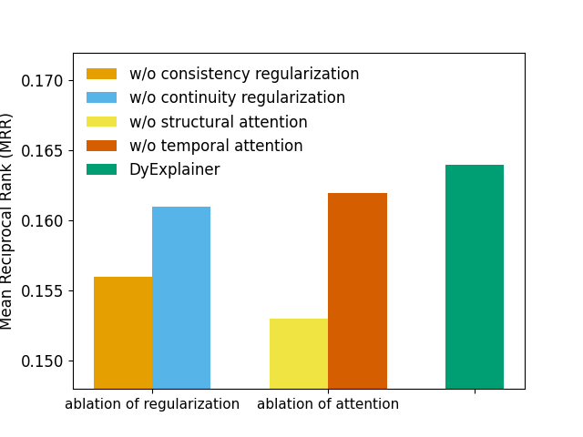
Figure 3. Ablation studies on Bitcoin-Alpha.

4.4. Explanations Performance

In order to demonstrate the reliability of the explanations provided by DyExplainer, we conduct quantitative evaluations that compare our approach with various baselines across three datasets characterized by a limited number of edges: UCI-Message, Bitcoin-OTC, and Bitcoin-Alpha. Specifically, we adopt the Fidelity vs. Sparsity metrics for our evaluation, in accordance with the methodology described in (Pope et al., 2019; Yuan et al., 2021). The Fidelity metric assesses the accuracy with which the explanations reflect the significance of various factors to the model’s predictions, while the Sparsity metric quantifies the proportion of structures that are deemed critical by the explanation techniques. For a fair comparison, for all three methods, we use a trained dynamic GNN (You et al., 2022) as the base model to calculate the predicted probability.

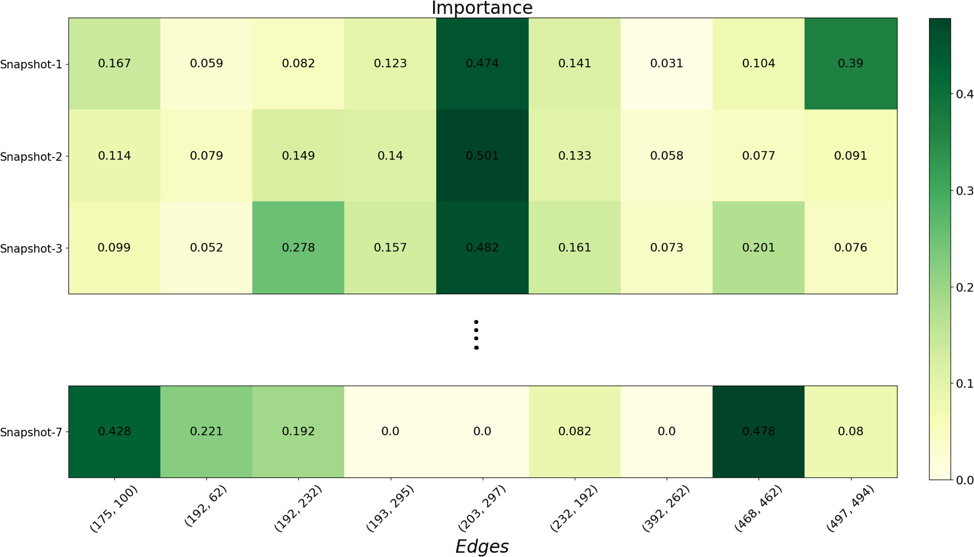
Figure 4. Heat map of edge importance over time. We sample some edges shared by continuous snapshots and show their attention values. 0.0 means this edge does not appear in this snapshot.

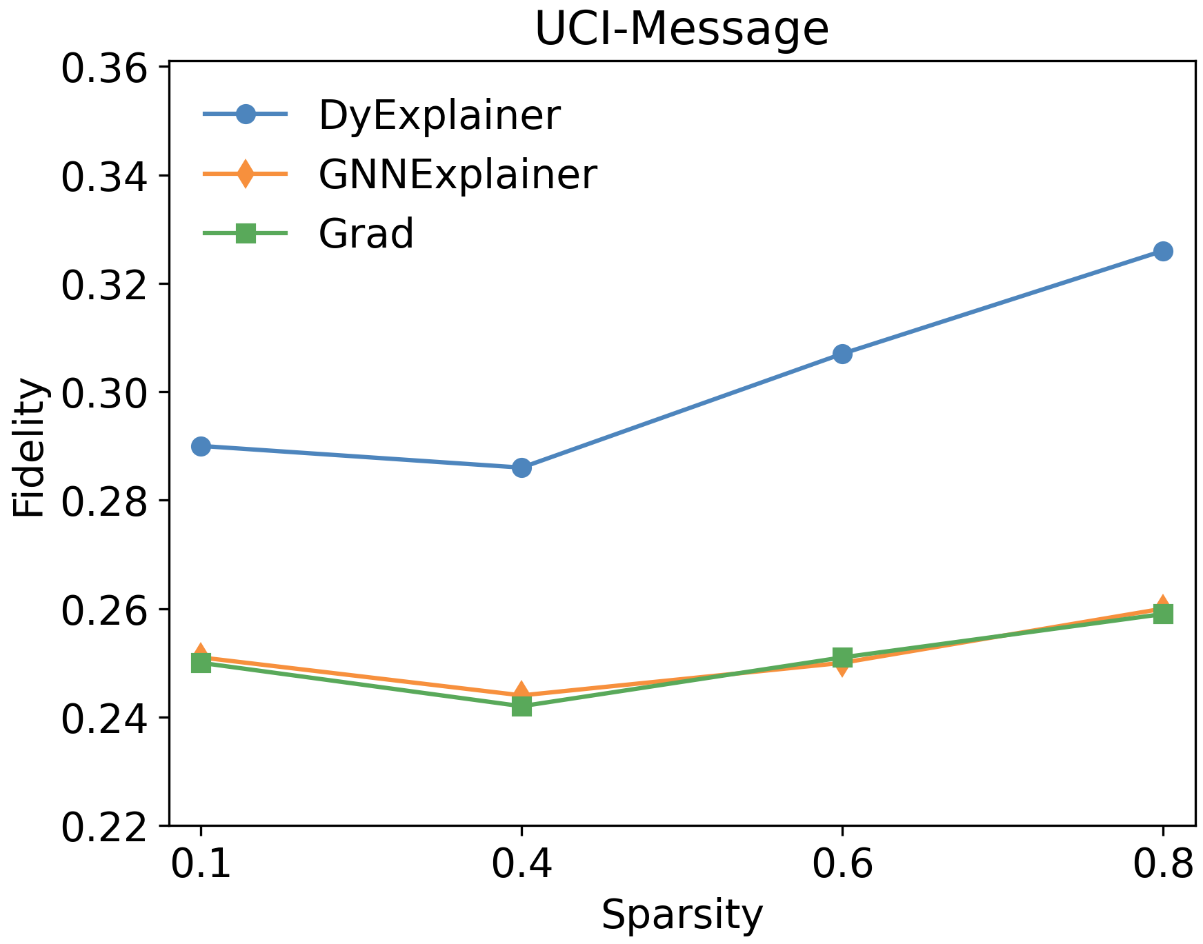
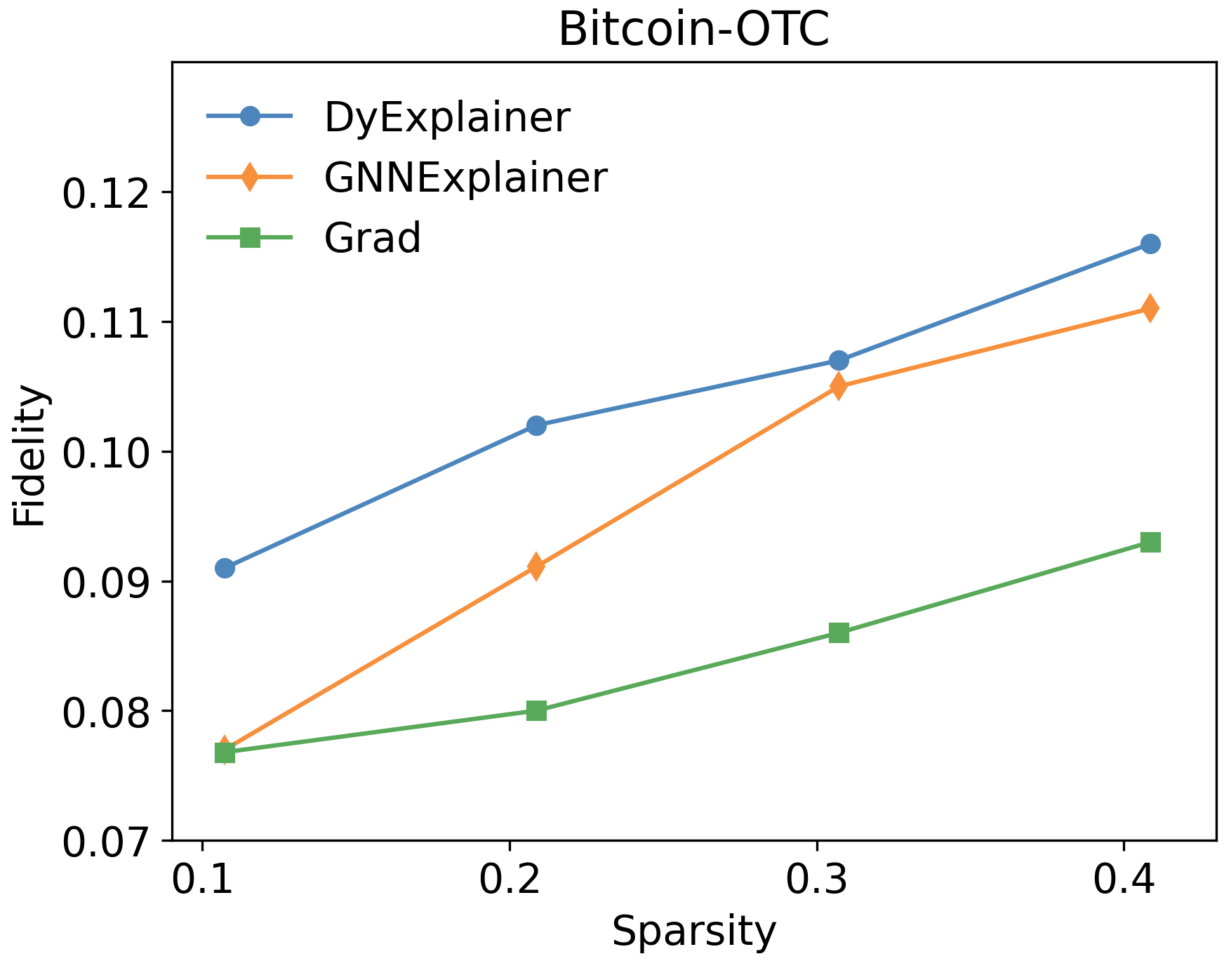
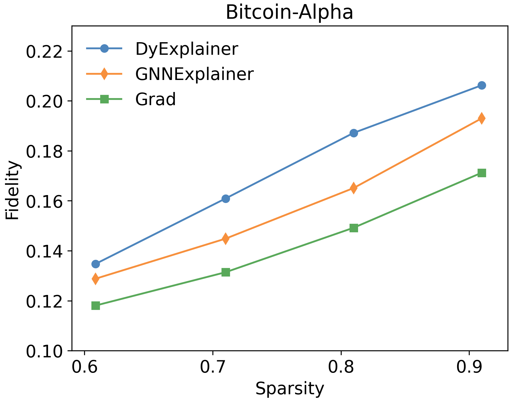
Figure 5. The quantitative studies for different explanation methods on UCI-Message, Bitcoin-OTC, and Bitcoin-Alpha.

The baseline method, GNNExplainer, was not originally developed for dynamic graph settings. Nevertheless, for a fair comparison, we assess the Fidelity of both DyExplainer and GNNExplainer using only the graph at the final snapshot, despite the fact that DyExplainer provides explanations for all snapshots stored in a buffer. GNNExplainer identifies the most influential nodes within a k-hop neighborhood and generates a mask to highlight these nodes for a given prediction node. As our DyExplainer provides a global attention mechanism for the entire graph, for a fair comparison, we calculate the average Fidelity of each mask produced by GNNExplainer with respect to all of the edges. To obtain the Fidelity and Sparsity metrics for each mask, we select a subset of the top-ranked edges based on the weights from the explanation mask and use this subset to create a new graph. The Fidelity of an edge is defined as the difference between the predicted probability of that edge on the new graph and the global graph. For DyExplainer, we directly select the top-ranked edges based on the attention weights to form a new graph, as there is only one global attention mechanism that provides the explanation.

The comparison of Fidelity and Sparsity is presented in Figure 5. The evaluation of various methods is based on their Fidelity scores under comparable levels of Sparsity, as the Sparsity level cannot be precisely controlled. From the figure, we see that for all three datasets, the Fidelity of these methods increases as Sparsity increases. This is due to the calculation of Fidelity as the difference between the predicted probability of the model on the reduced graph and the original graph, leading to higher Fidelity values with greater Sparsity. Furthermore, GNNExplainer demonstrates superior Fidelity compared to Grad on Bitcoin-OTC and Bitcoin-Alpha, while performing similarly on UCI-Message. Additionally, DyExplainer outperforms both methods on all three datasets at varying Sparsity levels, revealing that it provides more accurate explanations.

4.5. Case Studies

To show the evolving and continuity of underlying patterns the DyExplainer detects from the dynamic graph, we visualize the attention values of some edges at different snapshots on the Bitcoin-Alpha data set in Figure 4. From this figure, we observe that the edges $(192,62)$, $(193,295)$, $(203,297)$ and $(232,192)$ has close importance on snapshots 1-3. It indicates the temporal continuity of edge importance exists in dynamic graphs and our intuition is reasonable. The edges $(175,100)$, $(192,62)$, and $(468,462)$ are less important at snapshots 1-3 while becoming more important at snapshot 7. It infers that the importance of an edge is evolving along with the time steps.

We further visualize the temporal attention to show which historical snapshot has more influence on the current. The importance of snapshots provided by the temporal attention is shown in Figure 6. From the figure, we see that the most important snapshot to the current is snapshot 32.

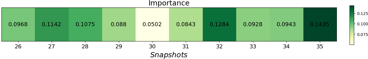
Figure 6. Heat map of temporal importance over time. The current snapshot is at 35. The buffer size is set to 10. It means we consider the importance of the previous snapshot from 27 to 34.

To see how the patterns have an effect, we randomly pick an edge $(623,26)$ at snapshot 35 to investigate the local structure of this edge at snapshot 32. The visualization of nodes 623 and 26 are shown in Figure 7. Note that these two nodes are unconnected at snapshot 32. The widths of edges are according to the weights of structural attention. Thicker ones mean large weights. From the figure, we can find that there are three clusters of substructures with larger weights, which can be viewed as important patterns that DyExplainer detects.

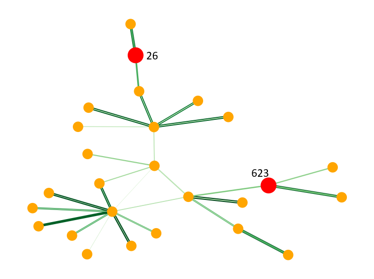
Figure 7. Local structure of node 26 and 623 (red nodes) on snapshot 32. Orange points are their 3-hop neighborhoods. The green edges are obtained from the structural attention weights at snapshot 32.

5. Related Work

The goal of explainability in GNNs is to provide transparency and accountability in the predictions of the models, especially when they are used in critical applications such as detecting the fraud (Liu et al., 2021) or medical diagnosis (Liu et al., 2020). Recently, many works are proposed to explain the GNN predictions, with a focus on diverse facets of the models from various perspectives. According to the type of explanation they provide, the methodologies can be categorized into two main classes: instance-level and model-level methods (Yuan et al., 2022).

The instance-level methods explain the GNN models by identifying the most influential features of the graph to the given prediction. Among them, some methods employ the gradients or the feature values to indicate the importance of features. SA (Baldassarre and Azizpour, 2019) computes the gradient value as the importance score for each input feature. While it is easy to compute by the back-propagation, the results cannot accurately capture the importance of each feature due to the output changing minimally with respect to the input change, and a gradient value is hard to reflect the input contribution. CAM (Pope et al., 2019) maps the node features in the final layer to the input space to identify important nodes. However, the representation from the final layer of GNN may not reflect the node contribution because the feature distribution may change after mapping by a neural network. Another kind of method aims to provide instance-level explanations by a surrogate model that approximates the predictions of the original GNN model. GraphLime (Huang et al., 2022) provides a model-agnostic local explanation framework for the node classification task. It adopts the node feature and predicted labels in the K-hop neighbors of the predicted node and trains an HSIC Lasso. GNNExplainer (Ying et al., 2019) takes a trained GNN and its predictions as inputs to provide explanations for a given instance, e.g. a node or a graph. The explanation includes a compact subgraph structure and a small subset of node features that are crucial in GNN’s prediction for the target instance. However, the explanation provided by GNNExplainer is limited to a single instance, making GNNExplainer difficult to be applied in the inductive setting because the explanations are hard to generalize to other unexplained nodes. PGExplainer (Luo et al., 2020) is proposed to provide a global understanding of predictions made by GNNs. It models the underlying structure as edge distributions where the explanatory graph is sampled. To explain the predictions of multiple instances, the generation process in PGExplainer is parameterized by a neural network. Similar to the PGExplainer, GraphMask (Schlichtkrull et al., 2020) trains a classifier to predict whether an edge can be dropped without affecting the original predictions. As a post-hoc method, GraphMask obtains an edge mask for each GNN layer. SubgraphX (Yuan et al., 2021) explains the GNN predictions as an efficient exploration of different subgraphs with Monte Carlo tree search. It adopts Shapley values as a measure of subgraph importance that also capture the interactions among different subgraphs. All of these methods are to provide explanations with respect to the GNN predictions. Different from them, this work provides a high-level understanding to explain the GNN models. The model-level methods that study what graph patterns can lead to a certain GNN behavior, e.g., the improvement of performance, is particularly related to us. There are fewer studies in this field. The method XGNN (Yuan et al., 2020) aims to explain GNNs by training a graph generator so that the generated graph patterns maximize a certain prediction of the model. The explanations by XGNN are general that provide a global understanding of the trained GNNs.

Current explainers for GNNs are limited to static graphs, hindering their application in dynamic scenarios. The explanation of dynamic GNNs is an under-studied area. Indeed, there is a recent work (Xie et al., 2022) attempted to provide explanations on dynamic graphs by exploring backward relevance, but it is limited to a specific model TGCN. Besides, the work in (He et al., 2022) considers explaining time series predictions by temporal GNNs. The work (Fan et al., 2021) learns attention weights for a linear combination of node representations dynamic graphs, but it explains the model by detecting the node importance. There are distinct challenges in explaining dynamic GNNs in general. Firstly, existing explanation methods mainly focus on identifying the important parts of the data in relation to the GNN predictions. However, dynamic GNNs make predictions for each snapshot, making it difficult to provide explanations for a particular prediction as it depends on all previous snapshots. Secondly, it is challenging to provide a generalizable solution to interpret various types of dynamic GNNs. DyExplainer, on the other hand, provides model-level explanations for all dynamic GNNs, overcoming these limitations.

6. Conclusion

We present DyExplainer, a pioneering approach to explaining dynamic GNNs in real-time. DyExplainer leverages a dynamic GNN backbone to extract representations at each snapshot, concurrently exploring structural relationships and temporal dependencies through a sparse attention mechanism. To ensure structural consistency and temporal continuity in the explanation, our approach incorporates contrastive learning techniques and a buffer-based live-updating scheme. The results of our experiments showcase the superiority of DyExplainer, providing a faithful explanation of the model predictions while concurrently improving the accuracy of the model, as evidenced by the link prediction task.

References

- (1)
- Baldassarre and Azizpour (2019) Federico Baldassarre and Hossein Azizpour. 2019. Explainability techniques for graph convolutional networks. Preprint arXiv:1905.13686 (2019).
- Cho et al. (2014) Kyunghyun Cho, Bart Van Merriënboer, Dzmitry Bahdanau, and Yoshua Bengio. 2014. On the properties of neural machine translation: Encoder-decoder approaches. arXiv preprint arXiv:1409.1259 (2014).
- Defferrard et al. (2016) Michaël Defferrard, Xavier Bresson, and Pierre Vandergheynst. 2016. Convolutional neural networks on graphs with fast localized spectral filtering. NIPS 29 (2016).
- Fan et al. (2021) Yucai Fan, Yuhang Yao, and Carlee Joe-Wong. 2021. Gcn-se: Attention as explainability for node classification in dynamic graphs. In 2021 IEEE International Conference on Data Mining (ICDM). IEEE, 1060–1065.
- Fey and Lenssen (2019) Matthias Fey and Jan Eric Lenssen. 2019. Fast graph representation learning with PyTorch Geometric. RLGM@ICLR (2019).
- He et al. (2022) Wenchong He, Minh N Vu, Zhe Jiang, and My T Thai. 2022. An explainer for temporal graph neural networks. In GLOBECOM. IEEE, 6384–6389.
- Hochreiter and Schmidhuber (1997) Sepp Hochreiter and Jürgen Schmidhuber. 1997. Long short-term memory. Neural computation 9, 8 (1997), 1735–1780.
- Huang et al. (2022) Qiang Huang, Makoto Yamada, Yuan Tian, Dinesh Singh, and Yi Chang. 2022. Graphlime: Local interpretable model explanations for graph neural networks. IEEE Transactions on Knowledge and Data Engineering (2022).
- Jang et al. (2016) Eric Jang, Shixiang Gu, and Ben Poole. 2016. Categorical reparameterization with gumbel-softmax. Preprint arXiv:1611.01144 (2016).
- Kipf and Welling (2016) Thomas N Kipf and Max Welling. 2016. Semi-supervised classification with graph convolutional networks. Preprint arXiv:1609.02907 (2016).
- Kumar et al. (2018a) Srijan Kumar, William L Hamilton, Jure Leskovec, and Dan Jurafsky. 2018a. Community interaction and conflict on the web. In WWW. 933–943.
- Kumar et al. (2018b) Srijan Kumar, Bryan Hooi, Disha Makhija, Mohit Kumar, Christos Faloutsos, and VS Subrahmanian. 2018b. Rev2: Fraudulent user prediction in rating platforms. In WSDM. 333–341.
- Kumar et al. (2016) Srijan Kumar, Francesca Spezzano, VS Subrahmanian, and Christos Faloutsos. 2016. Edge weight prediction in weighted signed networks. In ICDM. IEEE, 221–230.
- Leskovec et al. (2005) Jure Leskovec, Jon Kleinberg, and Christos Faloutsos. 2005. Graphs over time: densification laws, shrinking diameters and possible explanations. In ACM SIGKDD. 177–187.
- Leskovec and Krevl (2014) Jure Leskovec and Andrej Krevl. 2014. SNAP Datasets: Stanford Large Network Dataset Collection. http://snap.stanford.edu/data.
- Liang et al. (2022) Ke Liang, Lingyuan Meng, Meng Liu, Yue Liu, Wenxuan Tu, Siwei Wang, Sihang Zhou, Xinwang Liu, and Fuchun Sun. 2022. Reasoning over different types of knowledge graphs: Static, temporal and multi-modal. Preprint arXiv:2212.05767 (2022).
- Liu et al. (2023) Meng Liu, Yue Liu, Ke Liang, Siwei Wang, Sihang Zhou, and Xinwang Liu. 2023. Deep Temporal Graph Clustering. Preprint arXiv:2305.10738 (2023).
- Liu et al. (2021) Yang Liu, Xiang Ao, Zidi Qin, Jianfeng Chi, Jinghua Feng, Hao Yang, and Qing He. 2021. Pick and choose: a GNN-based imbalanced learning approach for fraud detection. In WWW. 3168–3177.
- Liu et al. (2020) Zheng Liu, Xiaohan Li, Hao Peng, Lifang He, and S Yu Philip. 2020. Heterogeneous similarity graph neural network on electronic health records. In Big Data. IEEE, 1196–1205.
- Louizos et al. (2017) Christos Louizos, Max Welling, and Diederik P Kingma. 2017. Learning Sparse Neural Networks through Regularization. Preprint arXiv:1712.01312 (2017).
- Luo et al. (2020) Dongsheng Luo, Wei Cheng, Dongkuan Xu, Wenchao Yu, Bo Zong, Haifeng Chen, and Xiang Zhang. 2020. Parameterized explainer for graph neural network. Advances in neural information processing systems 33 (2020), 19620–19631.
- Ma et al. (2019) Yao Ma, Suhang Wang, Charu C Aggarwal, and Jiliang Tang. 2019. Graph convolutional networks with eigenpooling. In Proceedings of the 25th ACM SIGKDD international conference on knowledge discovery & data mining. 723–731.
- Maddison et al. (2016) Chris J Maddison, Andriy Mnih, and Yee Whye Teh. 2016. The concrete distribution: A continuous relaxation of discrete random variables. arXiv preprint arXiv:1611.00712 (2016).
- McPherson et al. (2001) Miller McPherson, Lynn Smith-Lovin, and James M Cook. 2001. Birds of a feather: Homophily in social networks. Annual review of sociology 27, 1 (2001), 415–444.
- Nauta et al. (2022) Meike Nauta, Jan Trienes, Shreyasi Pathak, Elisa Nguyen, Michelle Peters, Yasmin Schmitt, Jörg Schlötterer, Maurice van Keulen, and Christin Seifert. 2022. From Anecdotal Evidence to Quantitative Evaluation Methods: A Systematic Review on Evaluating Explainable AI. arXiv preprint arXiv:2201.08164 (2022).
- Panzarasa et al. (2009) Pietro Panzarasa, Tore Opsahl, and Kathleen M Carley. 2009. Patterns and dynamics of users’ behavior and interaction: Network analysis of an online community. Journal of the American Society for Information Science and Technology 60, 5 (2009), 911–932.
- Pareja et al. (2020) Aldo Pareja, Giacomo Domeniconi, Jie Chen, Tengfei Ma, Toyotaro Suzumura, Hiroki Kanezashi, Tim Kaler, Tao Schardl, and Charles Leiserson. 2020. Evolvegcn: Evolving graph convolutional networks for dynamic graphs. In AAAI, Vol. 34. 5363–5370.
- Paszke et al. (2019) Adam Paszke, Sam Gross, Francisco Massa, Adam Lerer, James Bradbury, Gregory Chanan, Trevor Killeen, Zeming Lin, Natalia Gimelshein, Luca Antiga, et al. 2019. Pytorch: An imperative style, high-performance deep learning library. Advances in neural information processing systems 32 (2019).
- Pedregosa et al. (2011) Fabian Pedregosa, Gaël Varoquaux, Alexandre Gramfort, Vincent Michel, Bertrand Thirion, Olivier Grisel, Mathieu Blondel, Peter Prettenhofer, Ron Weiss, Vincent Dubourg, et al. 2011. Scikit-learn: Machine learning in Python. Journal of Machine Learning Research 12 (2011), 2825–2830.
- Peng et al. (2020) Hao Peng, Hongfei Wang, Bowen Du, Md Zakirul Alam Bhuiyan, Hongyuan Ma, Jianwei Liu, Lihong Wang, Zeyu Yang, Linfeng Du, Senzhang Wang, et al. 2020. Spatial temporal incidence dynamic graph neural networks for traffic flow forecasting. Information Sciences 521 (2020), 277–290.
- Pope et al. (2019) Phillip E Pope, Soheil Kolouri, Mohammad Rostami, Charles E Martin, and Heiko Hoffmann. 2019. Explainability methods for graph convolutional neural networks. In CVPR. 10772–10781.
- Rossi et al. (2020) Emanuele Rossi, Ben Chamberlain, Fabrizio Frasca, Davide Eynard, Federico Monti, and Michael Bronstein. 2020. Temporal graph networks for deep learning on dynamic graphs. arXiv preprint arXiv:2006.10637 (2020).
- Rudin et al. (2022) Cynthia Rudin, Chaofan Chen, Zhi Chen, Haiyang Huang, Lesia Semenova, and Chudi Zhong. 2022. Interpretable machine learning: Fundamental principles and 10 grand challenges. Statistics Surveys 16 (2022).
- Schlichtkrull et al. (2020) Michael Sejr Schlichtkrull, Nicola De Cao, and Ivan Titov. 2020. Interpreting graph neural networks for nlp with differentiable edge masking. Preprint arXiv:2010.00577 (2020).
- Seo et al. (2018) Youngjoo Seo, Michaël Defferrard, Pierre Vandergheynst, and Xavier Bresson. 2018. Structured sequence modeling with graph convolutional recurrent networks. In ICONIP. Springer, 362–373.
- Tonekaboni et al. (2021) Sana Tonekaboni, Danny Eytan, and Anna Goldenberg. 2021. Unsupervised Representation Learning for Time Series with Temporal Neighborhood Coding. In ICLR.
- Vaswani et al. (2017) Ashish Vaswani, Noam Shazeer, Niki Parmar, Jakob Uszkoreit, Llion Jones, Aidan N Gomez, Łukasz Kaiser, and Illia Polosukhin. 2017. Attention is all you need. Advances in neural information processing systems 30 (2017).
- Veličković et al. (2017) Petar Veličković, Guillem Cucurull, Arantxa Casanova, Adriana Romero, Pietro Lio, and Yoshua Bengio. 2017. Graph attention networks. Preprint arXiv:1710.10903 (2017).
- Vu and Thai (2020) Minh Vu and My T Thai. 2020. Pgm-explainer: Probabilistic graphical model explanations for graph neural networks. NeurIPS 33 (2020), 12225–12235.
- Wang et al. (2020) Xiaoyang Wang, Yao Ma, Yiqi Wang, Wei Jin, Xin Wang, Jiliang Tang, Caiyan Jia, and Jian Yu. 2020. Traffic flow prediction via spatial temporal graph neural network. In Proceedings of The Web Conference 2020. 1082–1092.
- Wu et al. (2022) Shiwen Wu, Fei Sun, Wentao Zhang, Xu Xie, and Bin Cui. 2022. Graph neural networks in recommender systems: a survey. Comput. Surveys 55, 5 (2022), 1–37.
- Xie et al. (2022) Jiaxuan Xie, Yezi Liu, and Yanning Shen. 2022. Explaining Dynamic Graph Neural Networks via Relevance Back-propagation. Preprint arXiv:2207.11175 (2022).
- Xin et al. (2022) Rui Xin, Chudi Zhong, Zhi Chen, Takuya Takagi, Margo Seltzer, and Cynthia Rudin. 2022. Exploring the Whole Rashomon Set of Sparse Decision Trees. In NeurIPS.
- Ying et al. (2019) Zhitao Ying, Dylan Bourgeois, Jiaxuan You, Marinka Zitnik, and Jure Leskovec. 2019. Gnnexplainer: Generating explanations for graph neural networks. In NeurIPS. 9240–9251.
- Ying et al. (2018) Zhitao Ying, Jiaxuan You, Christopher Morris, Xiang Ren, Will Hamilton, and Jure Leskovec. 2018. Hierarchical graph representation learning with differentiable pooling. Advances in neural information processing systems 31 (2018).
- You et al. (2022) Jiaxuan You, Tianyu Du, and Jure Leskovec. 2022. ROLAND: graph learning framework for dynamic graphs. In ACM SIGKDD. 2358–2366.
- Yu et al. (2017) Bing Yu, Haoteng Yin, and Zhanxing Zhu. 2017. Spatio-temporal graph convolutional networks: A deep learning framework for traffic forecasting. arXiv preprint arXiv:1709.04875 (2017).
- Yuan et al. (2020) Hao Yuan, Jiliang Tang, Xia Hu, and Shuiwang Ji. 2020. Xgnn: Towards model-level explanations of graph neural networks. In ACM SIGKDD. 430–438.
- Yuan et al. (2022) Hao Yuan, Haiyang Yu, Shurui Gui, and Shuiwang Ji. 2022. Explainability in graph neural networks: A taxonomic survey. IEEE Transactions on Pattern Analysis and Machine Intelligence (2022).
- Yuan et al. (2021) Hao Yuan, Haiyang Yu, Jie Wang, Kang Li, and Shuiwang Ji. 2021. On explainability of graph neural networks via subgraph explorations. In ICML. PMLR, 12241–12252.
- Zhang and Chen (2018) Muhan Zhang and Yixin Chen. 2018. Link prediction based on graph neural networks. NeurIPS 31 (2018).
- Zhao et al. (2019) Ling Zhao, Yujiao Song, Chao Zhang, Yu Liu, Pu Wang, Tao Lin, Min Deng, and Haifeng Li. 2019. T-gcn: A temporal graph convolutional network for traffic prediction. IEEE Transactions on Intelligent Transportation Systems 21, 9 (2019), 3848–3858.