Pauli resonance states in light nuclei: how they appear and how they can be eliminated

Abstract

Systematic analysis of parameters and properties of the Pauli resonance states are performed for light nuclei ⁶Li, ⁷Li, ⁸Be, ⁹Be and ¹⁰B, which are treated as two-cluster systems. The Pauli resonance states are redundant solutions of the resonating group method appearing when one try use more advanced description of the internal structure of interacting clusters. Our calculations are performed in a standard and advanced versions of the resonating group method. The standard version employs wave functions of many-particle shell model to describe internal motion of nucleons within each cluster. The advanced version is based on three-cluster resonating group method. As in the standard version, the internal wave functions of three clusters are approximated by wave functions of many-particle shell model model. However, in advanced version one of pair of clusters forms a bound state, and third cluster is considered to interact with such state. It is found that the Pauli resonance states in nuclei under consideration have energy between 11 and 46 MeV, and their widths vary from 8 keV to 6.7 MeV. Analysis of wave functions of Pauli resonance states and matrix elements of norm kernel allowed us to formulate an effective method for eliminating Pauli resonance states. It is demonstrated that this method effectively eliminate all determined the Pauli resonance states.

I Introduction

We are going to study properties of so-called Pauli resonance states, which have been numerously observed in Refs. Clement et al. (1974); Spitz et al. (1981); Kanada et al. (1975a, b); Fliessbach and Walliser (1982); Kanada et al. (1982); Stubeda et al. (1982); Fujiwara and Tang (1983); Walliser and Fliessbach (1983); Walliser et al. (1985); Kanada et al. (1988); Kruglanski and Baye (1992) and many others. These resonance states appear within the resonating group method (RGM) when one tries to use more realistic description of interacting nuclei (clusters). They have been considered as redundant solutions of equations of the resonating group method. As the Pauli resonance states appear not in all realizations (versions) of the resonating group method, we start with a short classification of main versions of the RGM, which are relevant to the subject of the present paper. The main difference of these methods is in the form of the wave function, which is used to approximate cluster structure of a compound nucleus. The standard version of the RGM suggests the following form of wave function of a two-cluster system of $A$ nucleons for the partition $A=A_{1}+A_{2}$

$$\Psi\left(A\right)=\widehat{\mathcal{A}}\left\{\Phi_{1}\left(A_{1},b\right)\Phi_{2}\left(A_{2},b\right)\psi\left(\mathbf{x}\right)\right\},$$ (1)

where $\mathbf{x}$ is a distance between centers of mass of clusters, $\psi\left(\mathbf{x}\right)$ is a wave function of relative motion of clusters, $\Phi_{1}\left(A_{1},b\right)$ and $\Phi_{2}\left(A_{2},b\right)$ are wave functions of the many-particle shell model describing motion of nucleons within the first and second cluster, respectively. They are antisymmetric and translationally invariant. Oscillator length $b$ determines effective size of clusters. An important component of Eq. (1) is the antisymmetrization operator $\widehat{\mathcal{A}}$ which makes antisymmetric wave function of a compound system. For the sake of brevity, we omit all quantum numbers. They will be explicitly indicated in Sec. II.

In second version which we call improved one wave function is chosen in the form

$$\Psi\left(A\right)=\widehat{\mathcal{A}}\left\{\Phi_{1}\left(A_{1},b_{1}\right)\Phi_{2}\left(A_{2},b_{2}\right)\psi\left(\mathbf{x}\right)\right\},$$ (2)

where different oscillator length $b_{1}$ and $b_{2}$ are used to improve description of the internal structure of each cluster. This version is suitable for clusters with large difference of masses, i.e., for example, when $A_{1}\gg A_{2}$.

The third version is called advanced version of the RGM and related to advanced description of the internal structure of one

$$\Psi\left(A\right)=\widehat{\mathcal{A}}\left\{\Phi_{1}\left(A_{1},b_{1}\right)\Psi_{2}\left(A_{2},b\right)\psi\left(\mathbf{x}\right)\right\},$$ (3)

or two clusters

$$\Psi\left(A\right)=\widehat{\mathcal{A}}\left\{\Psi_{1}\left(A_{1},b\right)\Psi_{2}\left(A_{2},b\right)\psi\left(\mathbf{x}\right)\right\}.$$ (4)

Contrary to the wave function $\Phi_{\alpha}\left(A_{\alpha},b\right)$ ($\alpha$=1,2), the wave function $\Psi_{\alpha}\left(A_{\alpha},b\right)$ is a solution of two-cluster Schrödinger equation with clusterization $A_{\alpha}=A_{\alpha 1}+A_{\alpha 2}$ and is presented in the form similar to (1). This version of the RGM suggests more correct description of compound system and is appropriate when one or both clusters $A_{1}$ and $A_{2}$ have an evident two-cluster structure or, in other words, they have weakly bound state(s) and thus can be easily split on two fragments. Many light nuclei, such as $d$, ⁶Li, ⁷Li, ⁷Be, have such properties as their separation energies are less than 3 MeV.

The Pauli resonance states have not seen in the standard version of the RGM. Only shape resonance states were detected within this version in a single-channel approximation. As it is well-known, shape resonances are created by the centrifugal and/or Coulomb barriers, and thus they lie relative close to the threshold of corresponding channel. The Pauli resonance states have been detected in the improved and advanced versions.

The most spectacular demonstration of the Pauli resonance states was presented in Refs. Walliser and Fliessbach (1983); Walliser et al. (1985), where elastic scattering of alpha particles on ¹⁶O has been calculated within standard and improved versions. Set of narrow and wide resonance states was emerged when different oscillator lengths (frequencies) were used for wave functions describing internal structure of ¹⁶O and ⁴He nuclei. They spread over a wide energy range from small to relatively high energies above the ¹⁶O+⁴He threshold. In light nuclei, within the advanced version of the RGM Clement et al. (1974); Spitz et al. (1981); Kanada et al. (1975a, b, 1982); Stubeda et al. (1982); Fujiwara and Tang (1983); Kanada et al. (1988) the Pauli resonance states have been observed at relatively high energy region $E>$15 MeV. It was also noticed in Ref. Spitz et al. (1981) that the Pauli resonance states manifest themselves in the states with small values of the total orbital momentum $L$.

Despite that the different authors have used different names for such type of resonances, such as ”positive energy bound states” Clement et al. (1974), ”redundant” Fliessbach and Walliser (1982) or ”spurious states” Stubeda et al. (1982), it was widely recognized that the correctly treated Pauli principle is the origin of those states.

Let us recall the main types of resonance states observed in many-particle and particular in nuclear systems. The first type is shape resonance states, they are created by centrifugal or/and Coulomb barriers. The second type is represented by the Feshbach resonance states. These resonance states appear due to a weak coupling between open and closed channels. There are two necessary conditions for creating the Feshbach resonances. A compound system should have at least two channels with different threshold energies, and there should be at least one bound state in the channel with larger threshold energy, provided that this channel is considered separately from the channel with lowest threshold energy.

The phenomenon which is called the Pauli resonance state cannot be explained by two main factors of creating of resonance states and thus cannot be attributed to the first or second types of resonances. It cannot be the Feshbach resonance as such resonance states observed in single-channel cases. It is impossible to relate the Pauli resonances to centrifugal or Coulomb barrier as they appear in states with zero or very small angular momenta, or they require very huge barrier.

The Pauli resonance states have been considered as redundant solutions of the RGM equations, and thus one needs to use an algorithm to eliminate these states. They distort real physical quantities, such as phase shifts, cross sections of different processes and so on. To our knowledge, there is only one algorithm for eliminating the Pauli resonance states formulated in Ref. Kruglanski and Baye (1992) and applied to the $\alpha$+¹⁶O system. We refer to this method as the REV method, which is stand for removing of eigenvalues of the norm kernel. It was suggested in Ref. Kruglanski and Baye (1992) to omit so-called almost forbidden Pauli states. A criterion was formulated how to distinguish such states from allowed states. This algorithm has eliminated all Pauli resonance states from the elastic scattering of alpha particles on ¹⁶O.

In the present paper we are going to examine continuous spectrum states of a set of light nuclei such as ⁶Li, ⁷Li, ⁷Be, ⁸Be, ⁹Be and ¹⁰B. All these nuclei are considered as a three-cluster configuration and treated within a three-cluster model formulated in Ref. Vasilevsky et al. (2009). The three-cluster configuration is than reduced to three (if all three clusters are different) or two (if two of three clusters are identical) binary channels. With such reduction, one pair of clusters forms a bound state, which within our method is described in a two-cluster approximation.

To study Pauli resonance states we will first of all analyze matrix of overlap and its eigenvalues for some set of light nuclei. Based on this analysis, we suggest an alternative method for eliminating the Pauli resonance states. This new method we call as the ROF method, it means Removing of Oscillator Functions. We will demonstrate that both method give close results and completely eliminate all Pauli resonance states.

The structure of the present paper is the following. In Section II we give a brief introduction to the methods applied to study properties of the Pauli resonances in light nuclei.In Section III the choice of input parameters and details of calculations are discussed. The manifestations of the Pauli resonance states in various two-cluster systems are demonstrated in Section III.1. The analysis of parameters of the Pauli resonance states and their wave functions is carried out in this section. Then in the Section III.5 we analyze behavior of matrix elements of the norm kernel and eigenvalues of the matrix. In Section IV we briefly explain main ideas of eliminating the Pauli resonance states suggested in Ref. Kruglanski and Baye (1992). Here we also demonstrate its efficiency. In Section V we formulate an alternative method for eliminating the Pauli resonance states and demonstrate how it works in two-cluster systems under consideration. Concluding remarks are presented in Section VI.

II Method

In this paper we will use two types of two-cluster functions and thus two realizations of the RGM. The first type of functions realizes the standard form of the resonating group method and the second type realizes the advanced form of the RGM. Wave function of the first type for partition $A=A_{1}+A_{2}$ are

$$\Psi_{E,J}\left(A\right)=\widehat{\mathcal{A}}\left\{\left\{\left[\Phi_{1}\left(A_{1},L_{1},S_{1},b\right)\Phi_{2}\left(A_{2},L_{2},S_{2},b\right)\right]_{S}\psi_{E,l,L,J}\left(x\right)Y_{l}\left(\widehat{\mathbf{x}}\right)\right\}_{L}\right\}_{J}$$ (5)

and wave functions of the second type for partition $A=A_{1}+A_{2}=A_{1}+\left(A_{21}+A_{22}\right)$ are

$$\Psi_{E,J}\left(A\right)=\widehat{\mathcal{A}}\left\{\left\{\left[\Phi_{1}\left(A_{1},L_{1},S_{1},b\right)\Psi_{2}\left(A_{2},L_{2},S_{2},b\right)\right]_{S}\psi_{E,l,J}\left(x\right)Y_{l}\left(\widehat{\mathbf{x}}\right)\right\}_{L}\right\}_{J},$$ (6)

where $\Psi_{2}\left(A_{2},S_{2},L_{2},b\right)$ is wave function of a bound state of two-cluster subsystem with partition $\left(A_{21}+A_{22}\right)$

$$\Psi_{2}\left(A_{2},L_{2},S_{2},b\right)=\widehat{\mathcal{A}}\left\{\left[\Phi_{1}\left(A_{21},S_{21},b\right)\Phi_{2}\left(A_{22},S_{22},b\right)\right]_{S_{2}}g_{\mathcal{E},\lambda,J}\left(y\right)Y_{\lambda}\left(\widehat{\mathbf{y}}\right)\right\}_{J}.$$ (7)

Recall, that in this paper we use capital letter $\Phi$ to denote wave functions that are not solutions of corresponding Schrödinger equation, they are wave functions of the many-particle shell model. These functions can be constructed as Slater determinants from a single-particle oscillator orbitals. The capital and small letters $\Psi$ and $\psi$ represent solutions of the many-particle Schrödinger equation or corresponding integro-differential Wheeler equation Wheeler (1937a, b).

One can see that we use $LS$ coupling scheme when the total spin $S$ is a vector sum of spins of clusters, and total orbital momentum $L$ is a vector sum of the orbital momenta of both clusters $L_{1}$ and $L_{2}$ and orbital moment of relative motion of clusters $l$.

In the present paper we consider special case of the advanced version of the RGM. The usage of the special case is justified by employing of a three-cluster model for investigating of a compound nucleus and a set of reactions proceeding through the nucleus. In this special case only one of two functions $\Psi_{1}$ and $\Psi_{2}$ of internal motion of nucleons is the solution of two-cluster Schrödinger equation, and another function is the many-body shell model wave functions. A four-cluster model will allow one to consider a general case with two wave functions $\Psi_{1}$ and $\Psi_{2}$ to be solutions of two-cluster Schrödinger equations.

To realize the advanced model, we employ of a three-model which was formulated in Refs. Vasilevsky et al. (2009); Nesterov et al. (2009). Within this model a three-cluster configuration is transformed into a set of binary channels, i.e. in several pairs of interacting nuclei, and one of the interacting nuclei is considered as a two-cluster system. In Refs. Vasilevsky et al. (2009); Nesterov et al. (2009) the model has been applied to study nuclei ⁷Be and ⁷Li with three-cluster configurations $\alpha+d+n$ and $\alpha+d+p$ respectively. The structure of the ¹⁰B nucleus has been investigated in Ref. Nesterov et al. (2014) by employing three-cluster configurations $\alpha+\alpha+d$. Recently, the model which involves two three-cluster configurations $\alpha+p+n$ and $t+d+p$ has been used in Ref. Kalzhigitov et al. (2021) to study resonance states of ⁶Li in a wide energy range.

The model involves the Gaussian basis to determine bound-state wave functions of two-cluster subsystems and oscillator basis to describe scattering of the third cluster on a bound state of two-cluster subsystem. The abbreviation AMGOB is used to distinguish this model. In the AMGOB, two-cluster (7) and three-cluster (6) wave functions are represented as

$$\Psi_{2}\left(A_{2},S_{2},L_{2},b\right)=\sum_{\nu=1}^{N_{G}}D_{\nu}^{E,L,J}\widehat{\mathcal{A}}\left\{\left[\Phi_{1}\left(A_{21},S_{21},b\right)\Phi_{2}\left(A_{22},S_{22},b\right)\right]_{S}G_{L}\left(x,b_{\nu}\right)Y_{L}\left(\widehat{\mathbf{x}}\right)\right\}_{J},$$ (8)

$$\Psi_{E,J}\left(A\right)=\sum_{n=0}^{N_{O}}C_{nL}^{E,J}\widehat{\mathcal{A}}\left\{\left[\Phi_{1}\left(A_{1},S_{1},b\right)\Psi_{2}\left(A_{2},S_{2},L_{2},b\right)\right]_{S,L_{2}}\Phi_{n,L}\left(y,b\right)Y_{L}\left(\widehat{\mathbf{y}}\right)\right\}_{J},$$ (9)

where

$$G_{L}\left(x,b_{\nu}\right)=\frac{1}{b_{\nu}^{3/2}}\sqrt{\frac{2}{\Gamma\left(L+3/2\right)}}\rho^{L}\exp\left\{-\frac{1}{2}\rho^{2}\right\},\qquad\left(\rho=\frac{x}{b_{\nu}}\right),$$ (10)

is the Gaussian function and

$$\Phi_{n,L}\left(y,b\right) = \left(-1\right)^{n}\mathcal{N}_{nL}~{}b^{-3/2}\rho^{L}e^{-\frac{1}{2}\rho^{2}}L_{n}^{L+1/2}\left(\rho^{2}\right),$$ (11)

$$\rho = \frac{y}{b},\quad\mathcal{N}_{nL}=\sqrt{\frac{2\Gamma\left(n+1\right)}{\Gamma\left(n+L+3/2\right)}},$$

is the oscillator function. In Eqs. (10) and (11), $b_{\nu}$ and $b$ denote oscillator lengths. Motivation for usage of these functions can be found in Ref. Vasilevsky et al. (2009). The expansion coefficients $D_{\nu}^{E,L,J}$ and $C_{nL}^{E,J}$ are solutions of a set of linear equations originated from corresponding Schrödinger equations. This is a system of equations for the expansion coefficients $D_{\nu}^{E,L,J}$

$$\sum_{\widetilde{\nu}=0}\left[\left\langle\nu,L\left|\widehat{H}^{\left(2\right)}\right|\widetilde{\nu},L\right\rangle-E\left\langle\nu,L|\widetilde{\nu},L\right\rangle\right]D_{\widetilde{\nu}}^{E,L,J}=0$$ (12)

and here is a system of equations for the expansion coefficients $C_{nL}^{E,J}$

$$\sum_{\widetilde{n}=0}\left[\left\langle n,L\left|\widehat{H}\right|\widetilde{n},L\right\rangle-E\left\langle n,L|\widetilde{n},L\right\rangle\right]C_{\widetilde{n}L}^{E,J}=0.$$ (13)

System of equations (12) involves matrix elements of the two-cluster Hamiltonian

$$\left\langle\nu,L\left|\widehat{H}^{\left(2\right)}\right|\widetilde{\nu},L\right\rangle$$

and unit operator (norm kernel) $\left\langle\nu,L|\widetilde{\nu},L\right\rangle$ between cluster Gaussian functions

$$\left|\nu,L\right\rangle=\widehat{\mathcal{A}}\left\{\left[\Phi_{1}\left(A_{1},S_{1},b\right)\Psi_{2}\left(A_{2},S_{2},L_{2},b\right)\right]_{S,L_{2}}G_{L}\left(x,b_{\nu}\right)Y_{L}\left(\widehat{\mathbf{y}}\right)\right\}_{J},$$ (14)

while system of equations (13) involves matrix elements of the three-cluster Hamiltonian $\left\langle n,L\left|\widehat{H}\right|\widetilde{n},L\right\rangle$ and unit operator $\left\langle n,L|\widetilde{n},L\right\rangle$ between cluster oscillator functions

$$\left|n,L\right\rangle=\widehat{\mathcal{A}}\left\{\left[\Phi_{1}\left(A_{1},S_{1},b\right)\Psi_{2}\left(A_{2},S_{2},L_{2},b\right)\right]_{S,L_{2}}\Phi_{n,L}\left(y,b\right)Y_{L}\left(\widehat{\mathbf{y}}\right)\right\}_{J}.$$ (15)

We will also use another basis of cluster oscillator functions

$$\left|n,L\right\rangle_{0}=\widehat{\mathcal{A}}\left\{\left[\Phi_{1}\left(A_{1},S_{1},b\right)\Phi_{2}\left(A_{2},S_{2},L_{2},b\right)\right]_{S,L_{2}}\Phi_{n,L}\left(y,b\right)Y_{L}\left(\widehat{\mathbf{y}}\right)\right\}_{J}$$ (16)

to expand wave functions of two-cluster systems in the standard version of the RGM (5). It is obvious, that the wave functions $\left|n,L\right\rangle_{0}$ are partial case of wave functions $\left|n,L\right\rangle$ when the second cluster has the most compact shape.

Appearance of the matrix $\left\|\left\langle n,L|\widetilde{n},L\right\rangle\right\|$ in Eq. (13) indicates that cluster oscillator basis (15) is not orthonormal, despite that all functions to the right of the antisymmetrization operator in Eq. (15) are normalized to unity on the corresponding part of coordinate space. This matrix plays an important role in cluster models. It reflects effects of the Pauli principle. If one neglects the total antisymmetrization by putting $\widehat{\mathcal{A}}=1$, one obtains unit matrix $\left\|\left\langle n,L|\widetilde{n},L\right\rangle\right\|$. When effects of the Pauli principle are small, than the diagonal matrix elements are close to unity and off-diagonal matrix elements tend to zero. Such behavior of matrix elements $\left\langle n,L|\widetilde{n},L\right\rangle$ is observed for large values of $n$ and $\widetilde{n}$. This region of quantum numbers $n$ and $\widetilde{n}$ corresponds to large distances between clusters and thus is called as asymptotic region.

In the standard version of the RGM, the matrix $\left\|\left\langle n,L|\widetilde{n},L\right\rangle\right\|$ is diagonal for two $s$-clusters. Within advanced version of the RGM, as will be demonstrated later, the matrix $\left\|\left\langle n,L|\widetilde{n},L\right\rangle\right\|$ is not diagonal, however, the largest matrix elements are situated on the main diagonal of the matrix.

It worthwhile noticing that the wave functions $\left\{C_{nL}^{E,J}\right\}$ obtained by solving the system of equations (13) are normalized by the conditions

$$\sum_{n,n=0}C_{nL}^{E_{\alpha},J}\left\langle n,L|\widetilde{n},L\right\rangle C_{\widetilde{n}L}^{E_{\alpha},J}=\delta_{\alpha\beta}$$ (17)

for states of discrete spectrum and

$$\sum_{n,n=0}C_{nL}^{E,J}\left\langle n,L|\widetilde{n},L\right\rangle C_{\widetilde{n}L}^{\widetilde{E},J}=\delta\left(E-\widetilde{E}\right)$$ (18)

for continuous spectrum states. An important consequence of Eqs. (17) and (18) is that the value $\left|C_{nL}^{E,J}\right|^{2}$ does not determine the contribution of the oscillator functions $\left|n,L\right\rangle$ to the norm of a bound state or continuous spectrum state.

To solve equation (13) for a finite number of basis functions ($n$=0, 1, 2, …, $N_{O}-1$), one needs to analyze the $N_{O}\times N_{O}$ matrix $\left\|\left\langle n,L|\widetilde{n},L\right\rangle\right\|$, whether this matrix contains redundant states, which are called the Pauli forbidden states. For this aim the diagonalization procedure is usually employed which yields the eigenvalues $\Lambda_{\alpha}$ ($\alpha$=1, 2, …, $N_{O}$) and corresponding eigenfunctions $\left\|U_{n}^{\alpha}\right\|$ of the matrix $\left\|\left\langle n,L|\widetilde{n},L\right\rangle\right\|$. Eigenstates with $\Lambda_{\alpha}=0$ are called the Pauli forbidden states and have to be removed from the space. Eigenstates with small values of $\Lambda_{\alpha}$ are called the partially or almost forbidden states. There are usually a large number of eigenstates with $\Lambda_{\alpha}=1$. These states are not affected by the antisymmetrization. Besides, the matrix $\left\|\left\langle n,L|\widetilde{n},L\right\rangle\right\|$ can have eigenvalues with $\Lambda_{\alpha}>1$, they are called the super allowed states.

Note that the construction of the Pauli allowed states is a key problem for many-cluster systems. Many algorithms have been formulated (see, for example, Horiuchi (1977); Fujiwara and Horiuchi (1980); Kato et al. (1988),) to construct and to select Pauli allowed states.

Actually, in our hands we have two different discrete representations of the Schrödinger equation. The first representation is the oscillator basis representation and will be referred as $n-$representation. The second representation is formed by eigenvalues of the norm kernel matrix and will be referred as $\alpha-$representation. It is necessary to recall that both representations are related by the orthogonal matrix $\left\|U_{n}^{\alpha}\right\|$.

In the $\alpha-$representation the set of equations (13) is transformed to the form

$$\sum_{\widetilde{\alpha}=1}^{N_{O}}\left[\left\langle\alpha,L\left|\widehat{H}\right|\widetilde{\alpha},L\right\rangle-E\Lambda_{\alpha}\delta_{\alpha,\widetilde{\alpha}}\right]C_{\widetilde{\alpha}L}^{E,J}=0,$$ (19)

where

$$\left\langle\alpha,L\left|\widehat{H}\right|\widetilde{\alpha},L\right\rangle=\sum_{n,\widetilde{n}=0}^{N_{O}}U_{n}^{\alpha}\left\langle n,L\left|\widehat{H}\right|\widetilde{n},L\right\rangle U_{\widetilde{n}}^{\widetilde{\alpha}}.$$ (20)

If the cluster system under consideration contains no the Pauli forbidden states, then one may use the set of equations (13) or (19), both sets give the same spectrum but different wave functions. One has to use the set of equations (19) when there are one or more the Pauli forbidden states.

To study effects of the Pauli principle we will analyze the overlap matrix $\left\|\left\langle n,L|\widetilde{n},L\right\rangle\right\|$, we will also analyze the eigenvalues and eigenfunctions of the matrix.

III Results and discussions

As was pointed above, we consider a set of light nuclei. In Table 1 we list these nuclei and present details of the model and calculations. Here 3C stands for a three-cluster configuration which is taken into consideration, BC indicates binary channels which are studied. The Minnesota potential Thompson et al. (1977) is used as a nucleon-nucleon potential. Oscillator length $b$ is chosen to minimize energy of three-cluster threshold. The exchange parameter $u$ of the MP is usually selected to reproduce energy of the ground state of a compound system, accounted from the lowest two- or three-body thresholds.

We employ four Gaussian function to obtain the energy and wave functions of two-cluster subsystems, and 100 oscillator functions to describe scattering of the third cluster on two-cluster subsystem. It was checked numerously, that such number of oscillator functions is sufficient to obtain the bound state energies of a compound nucleus and scattering parameters with acceptable precision.

Table 1: List of nuclei to be considered, their three-cluster configurations (3C) and binary channels (BC), and input parameters of calculations: oscillator length $b$, exchange parameter $u$ of the Minnesota potential

Nucleus	3C	BC	$b$	$u$	Source
6Li	$\alpha+p+n$	$\alpha+d$	1.285	0.863	Kalzhigitov et al. (2021)
	$t+d+p$	$t+^{3}$He
7Li	$\alpha+d+n$	$\alpha+^{3}$H, 6Li$+n$	1.311	0.956	Nesterov et al. (2009)
7Be	$\alpha+d+p$	$\alpha+^{3}$He, 6Li$+p$	1.311	0.956	Vasilevsky et al. (2009)
8Be	$\alpha+d+d$	6Li$+d$	1.311	0.956
9Be	$\alpha+t+d$	$t+^{6}$Li	1.285	0.950	Lashko et al. (2023)
10B	$\alpha+\alpha+d$	$d+^{8}$Be, $\alpha+^{6}$Li	1.298	0.900	Nesterov et al. (2014)

To consider properties of the Pauli resonances in more detail, we restricted ourselves to a single-channel approximation. Moreover, we do not consider mixture of states with different values of the total orbital momentum $L$ and total spin $S$, thus in our present model $L$ and $S$ are additional quantum numbers to the angular momentum $J$ and parity $\pi$ of a compound system. In this paper we will not consider many-channel cases. This is a subject for our next investigation.

III.1 Manifestation of the Pauli resonance states

In this section we show how the Pauli resonance states manifest themselves in nuclei under consideration. For this aim we consider phase shifts. The most typical picture is shown in Fig. 1 where phase shifts are displayed for four different $J^{\pi}$ states of the elastic $\alpha+t$ scattering. These phase shifts exhibit resonance states of two different types. The first type is the shape resonance states, they are created in the states 7/2^- and 5/2^-. These resonance states are formed by combination of a huge centrifugal barrier at the $L$=3 state and Coulomb barrier. The shape resonance states lie close to the $\alpha+t$ threshold. The second type is the Pauli resonances which exhibit themselves in the states 3/2^- and 1/2^-. Energies of the Pauli resonances are $E$=25.8 MeV for 3/2^- state and $E$=29.0 MeV for 1/2^- state. The total orbital momentum $L$=1 is responsible for these resonance states. It means that in these states the centrifugal barrier is approximately 6 smaller than in the 7/2^- and 5/2^- states. Thus the centrifugal barrier cannot be responsible for the Pauli resonance states. The phase shifts displayed in Fig. 1 are similar to the phase shifts which were shown in Fig. 1 of Ref. Clement et al. (1974). The improved version of the RGM has been used in Ref. Clement et al. (1974), and two different oscillator lengths were chosen for an alpha particle and a triton.

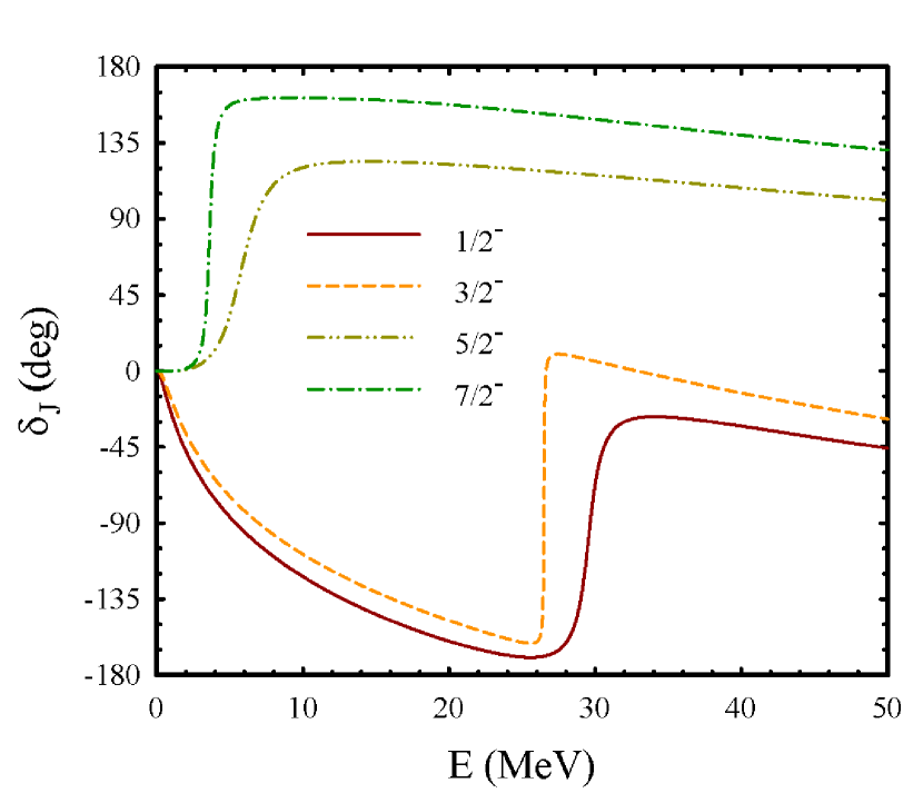
Figure 1: Phase shifts of the $\alpha+t$ elastic scattering in the states $J^{\pi}$ = 1/2^-, 3/2^-, 5/2^- and 7/2^-

Let us consider the Pauli resonance states in the 1⁺ ($L$=0, $S$=1) and 2^- ($L$=1, $S$=1) states of ⁶Li, which exhibit themselves in the channels ⁴He+$d$ and ³He+$t$. It is necessary to recall, that wave functions of deuteron and triton are obtained in two-cluster (two-body) approximations as $p+n$ and $d+n$, respectively. Such advanced description of deuteron and triton stipulate appearance of the Pauli resonance states, shown in Fig. 2. Only one Pauli resonance state is found in each channel. Energies and widths of these resonances depend on the total orbital momentum $J$.

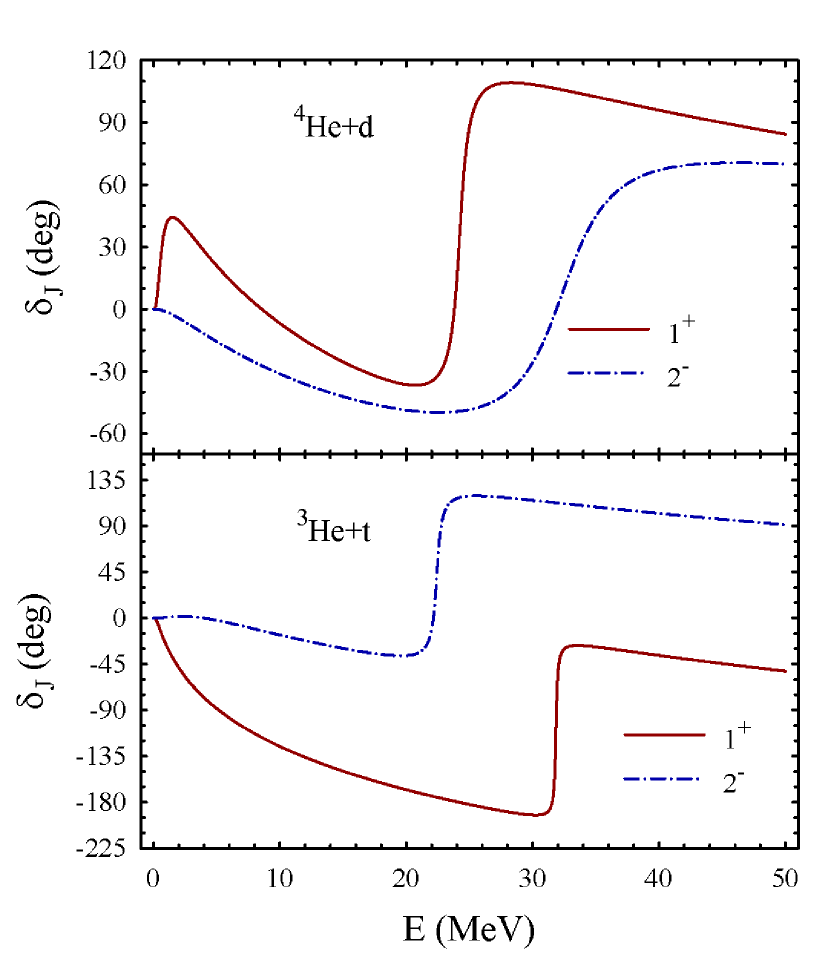
Figure 2: Phase shifts of the elastic ⁴He+$d$ and ³He+$t$ calculated for the 1⁺ and 2^- states in the advanced version of RGM

Another example of the Pauli resonance manifestation is shown in Fig. 3 for the ⁶Li+$\alpha$ scattering. This case demonstrates that two-cluster system may have two Pauli resonance states, they are located at energy range 10$\leq E\leq$45 MeV. A sharp growing of the 1⁺ phase shifts around 13.4 MeV indicates that there is very narrow resonance state with the widths $\Gamma$=56 keV. Other Pauli resonances are significantly wider.

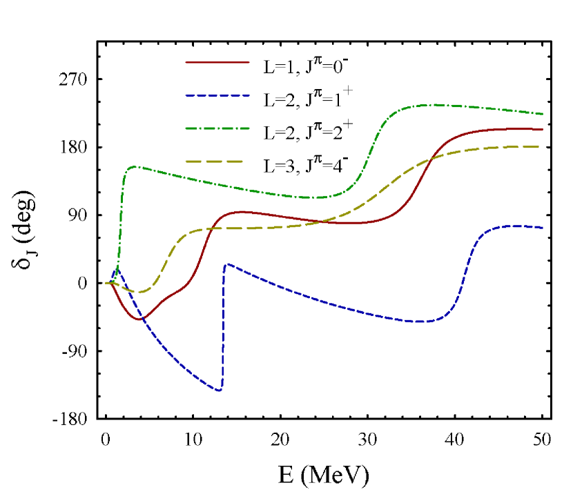
Figure 3: Phase shifts of the elastic ⁶Li+$\alpha$ scattering as a function of energy $E$.

In Fig. 4 we show phase shifts of the elastic ⁶Li+$d$ scattering with the total orbital momentum $L$=1 and total spin $S$=2. Due to the spin-orbital potential we obtain phase shifts for three states of the total angular momentum $J^{\pi}$ =3^-, 2^- and 1^-. Thus difference in behavior of phase shifts is totally originated from the spin-orbit potential. Fig. 4 demonstrates that energy and width of the Pauli resonance states depends on the spin-orbit components of nucleon-nucleon interaction. Indeed, we obtained that $E$=22.636 MeV, $\Gamma$=0.952 MeV for $J$=1^-, $E$=20.981 MeV, $\Gamma$=0.402 MeV for $J$=2^-, $E$=18.523 MeV, $\Gamma$=0.008 MeV for $J$=3^-. We see that spin-orbital potential substantially changes energy and width of the Pauli resonance states.

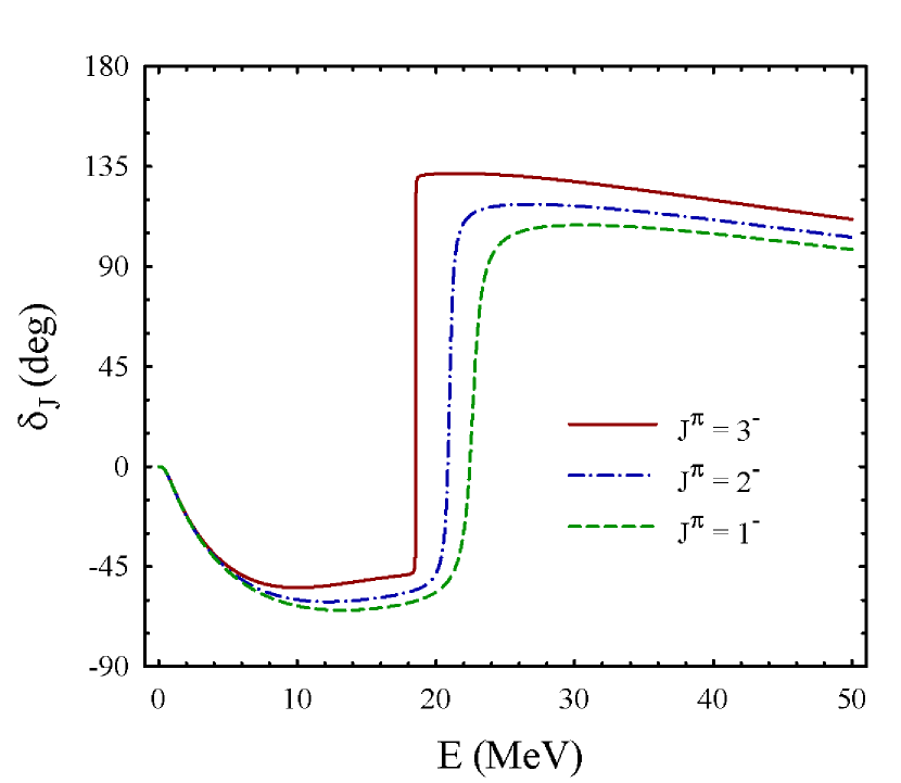
Figure 4: Phase shifts of the elastic ⁶Li+$d$ scattering as a function of energy. They obtained for $L$=1, $S$=2, and three values of the total angular momentum $J$.

Let us consider how central part of the MP affects energy and width of the Pauli resonance states. That can be done by varying the exchange parameter $u$ of that potential. This parameter affects interaction of nucleons in odd states, they also affects cluster-cluster interaction. The smaller is $u$, the smaller is interaction between clusters. When the parameter $u$ approaches to unity, interaction between clusters is increased. Influence of parameter $u$ variation is carried out for the 3/2^- state of ⁷Li considered as two-cluster system $\alpha+t$. Results of variation $u$ is demonstrated for the ground state energy $E_{GS}$, and for energy and width of the Pauli resonance. On can see in Fig. 5 that parameter $u$ changes energy of the ground state. Moreover, when $u<$0.86, the nucleus ⁷Li has no bound state. By varying parameter $u$ from 0.86 to 1, we change the ground state energy from -0.038 to -1.78 MeV. However, variation of $u$ from 0.8 to 1, reduces significantly energy of the Pauli resonance from 30.67 to 24.44 MeV. Such a variation of $u$ slightly changes width of the Pauli resonance state from 13 to 33 keV.

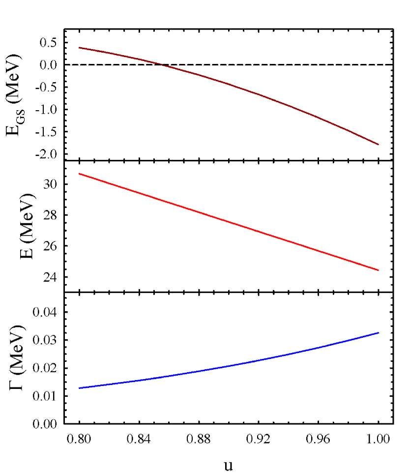
Figure 5: Dependence of the ground state energy $E_{GS}$ of ⁷Li, energy and width of the Pauli resonance state in the 3/2^- state of the $\alpha+t$ channel on the exchange parameter $u$ of the MP

III.2 Special case for $d+\alpha$ system

Taking into account peculiarities of our model, we decided to carry out an additional investigation of the $d+\alpha$ system. For this specific case our model allows to realize not only standard and advanced, but also improved version of the RGM. If we take only one Gaussian function in expansion of deuteron wave function, and select parameters $b_{0}$ (see Eq. (8)) to minimize the bound state energy of a deuteron, we realize therefore the improved version of the RGM. One Gaussian function with the optimal value of $b_{0}=$1.512 fm creates bound state of deuteron with energy $E$ =-0.132 MeV, while four Gaussian functions with optimal values of $b_{0}$ and $q$ generates the deuteron bound state with energy $E$ =-2.020 MeV.

To locate the Pauli resonance state in the approximation in the energy range below 50 MeV, we have to change the exchange parameter $u$ and take $u$=1.0. In Fig. 6 we show phase shift of the $d+\alpha$ scattering in $L$=0, $S$=1 $J^{\pi}=1^{+}$ state obtained in three approximations. Standard version of the RGM does not generate the Pauli resonance state in this case. The Pauli resonance states appear in the improved (I) and advanced (A) versions. Parameters of the Pauli resonance states substantially depends on a wave function describing internal structure of deuteron. More realistic wave function significantly increases width of the Pauli resonance (from $\Gamma=$0.001 MeV to $\Gamma=$1.718 MeV), and dramatically changes the energy (from $E=$47.55 MeV to $E=$22.49 MeV) of the resonance state in the state $J^{\pi}=1^{+}$.

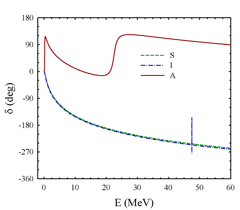
Figure 6: Phase shifts of the elastic $\alpha+d$ scattering in the state $L=0$, $S=1$, $J^{\pi}=$1⁺, obtained in three different approximations of the RGM

III.3 Main properties of the Pauli resonance states

In Table 2 we collect information on parameters of the Pauli resonance states detected in nuclei under consideration. It is detected 28 Pauli resonance states. The energy of resonance states is reckoned from the threshold of the channel indicated in column ”Channel” of Table 2 and is varying from 11 to 46 MeV. There are 10 narrow resonance states with $\Gamma<$1 MeV, six of them are very narrow resonance states with the width $\Gamma<$0.1 MeV. The rest 18 resonance states are wider ones, their widths exceed 1 MeV. One can see that in most cases two-cluster system with fixed quantum numbers $L$, $S$ and $J^{\pi}$ has only one Pauli resonance state. However, there are some cases when two Pauli resonance states are observed. The larger is energy of the resonance state, the larger is the total width. Energy of the second resonance state in ⁷Li and ⁸Be is approximately 15 MeV larger than the energy of the first resonance state. In ¹⁰B the energy difference is more than 25 MeV.

Table 2: Parameters of the Pauli resonance states in ⁶Li, ⁷Li and ¹⁰B

Nucleus	Channel	$L$	$S$	$J^{\pi}$	$E$, MeV	$\Gamma$, MeV
6Li	$\alpha+d$	0	1	1+	24.218	1.165
		1	1	2-	32.370	6.755
	3He$+t$	0	1	1+	31.844	0.209
		1	1	2-	22.403	0.618
7Li	$\alpha+t$	1	1/2	1/2-	29.002	2.144
		1	1/2	3/2-	25.810	0.027
		0	1/2	1/2+	20.148	2.589
		0	1/2	1/2+	34.444	4.702
	6Li$+n$	0	1/2	1/2+	12.863	3.332
		0	3/2	3/2+	18.895	0.196
10B	6Li$+\alpha$	1	1	0-	11.090	3.198
		1	1	0-	35.834	4.600
		1	1	1-	11.098	3.424
		1	1	1-	36.167	5.105
		0	1	1+	13.427	0.056
		0	1	1+	41.144	2.751

In Table 3 we present parameters of the Pauli resonance states obtained in different state of ⁶Li+$d$ and ⁷Li+$d$ scattering.

Table 3: Energies and widths of the Pauli resonance states in ⁸Be and ⁹Be observed in the channels ⁶Li+$d$ and ⁷Li+$d$, respectively

Nucleus	Channel	$L$	$S$	$J^{\pi}$	$E$, MeV	$\Gamma$, MeV
8Be	6Li+$d$	0	0	$0^{+}$	17.233	3.553
		0	1	$1^{+}$	14.989	1.011
		0	1	$1^{+}$	25.724	4.628
		0	2	$2^{+}$	20.656	0.008
		1	0	$1^{-}$	18.253	0.058
		1	1	$2^{-}$	45.555	6.097
		1	1	$2^{-}$	18.523	0.008
		1	2	$3^{-}$	18.531	0.013
		1	2	$2^{-}$	20.981	0.402
9Be	7Li+$d$	1	1/2	1/2-	13.733	1.003
		0	1/2	1/2+	15.717	5.796
		0	1/2	1/2+	27.958	1.836

By analyzing results presented in Tables 2 and 3, we came to the conclusion that the Pauli resonance states in light nuclei have energy more than 11 MeV, their widths are mainly large ($\Gamma>$0.9 MeV), however a few very narrow resonance state were found. The most populated area of resonance states lies in the interval 16$<E<$21 MeV, as it is demonstrated in Fig. 7, left panel. Two dense area of widths of resonance states are located in intervals 0.008 $<\Gamma<$0.22 MeV and 0.9$<\Gamma<$1.2 MeV (Fig. 7, right panel). In many cases only one Pauli resonance state appeared in a binary channel. We also determined several cases with two resonance states.

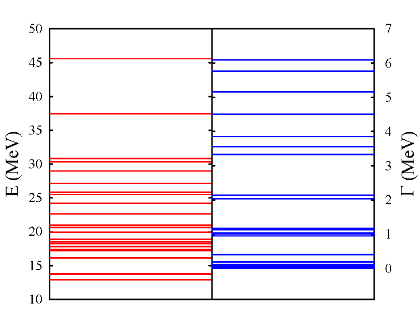
Figure 7: Density of resonance state energies (left panel) and widths (right panel) of all determined Pauli resonance states

In Fig. 8 we display spectrum of the Pauli resonances of positive parity states with the total orbital momentum $L=0$. These resonance states emerge in nuclei ⁷Li, ⁸Be, ⁹Be and ¹⁰B with clusterization ⁶Li+$A_{2}$, where $A_{2}$ stands for neutron, deuteron, triton and alpha particle. This Figure shows that the energies of the first Pauli resonance states are quite close for all nuclei. It also shows that there are two Pauli resonance states in the channel ⁶Li$+d$ with the total spin $S$=1 and in the channel ⁶Li$+t$ with the total spins $S$=1/2 and $S$=3/2. One can see that the larger is the second cluster, the larger is the energy of the highest Pauli resonance state. Indeed, it growths from 19 MeV in ⁶Li$+n$ channel to 41 MeV in the channel ⁶Li$+\alpha$.

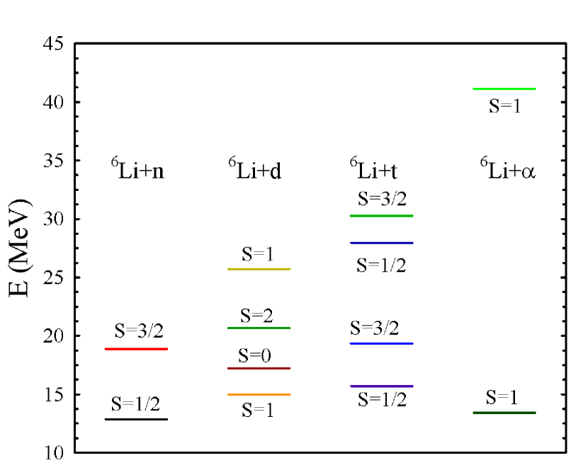
Figure 8: Spectrum of positive parity Pauli resonances for $L$=0 state of nuclei ⁷Li, ⁸Be, ⁹Be, ¹⁰B detected in the channels ⁶Li+$n$, ⁶Li+$d$, ⁶Li+$t$ and ⁶Li+$\alpha$, correspondingly

The Pauli resonance states of negative parity created in the channel ⁶Li+$A_{2}$ ($A_{2}$ =$d$, $t$, $\alpha$) with the total orbital momentum $L$=1 are show in Fig. 9. We did not find any resonance state in the channel ⁶Li+$n$. In this channel, the Pauli resonance states do not appear neither in states with total spin $S$=1/2 nor in the states $S$=3/2. Five Pauli resonance states are found in ⁸Be and ⁹Be, and four resonances are detected in ¹⁰B. Fig. 9 shows that the energy of the lowest Pauli resonance state is deceasing with increasing of mass of the ”projectile” $A_{2}$. It is interesting tendency, as the Coulomb repulsing between ⁶Li and $A_{2}$ is increased with increasing of mass of the second cluster $A_{2}$. It necessary to underline that the spin-orbit interaction plays an important role in all cases when both the total orbital momentum $L$ and total spin $S$ do not equal to zero.

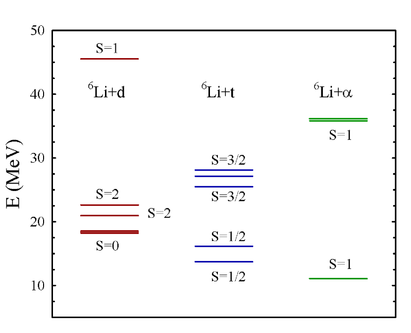
Figure 9: Spectrum of the Pauli resonance states of the negative parity in ⁸Be, ⁹Be and ¹⁰B created in the state with the total orbital momentum $L$=1.

III.3.1 Birth of the Pauli resonance state

To detect the Pauli and shape resonance states we analyzed behavior of phase shifts as a function of energy. Rapid growth of phase shift was considered as a signal of a resonance state. There is another way for detecting of resonance states of both types. This way applicable for any method which involve a square integrable basis of functions. Unfortunately this method works for relatively narrow resonance states. The narrow resonance states can be detected by calculating eigenspectrum of a Hamiltonian with different number of basis functions. By displaying eigenenergies as a function of the number of basis functions (we denote them as $N_{O}$) involved in calculations, a resonance state will display itself as a plateau or/and as a avoid crossing. Energy of plateau is the energy of a resonance state. Such way of detecting of resonance states is an essential element of the stabilization method (Ref. Hazi and Taylor (1970)) and complex scaling method (see definitions of the method and its recent progress in applications to many-cluster systems in Refs. Myo et al. (2014); Horiuchi et al. (2012); Myo and Katō (2020)).

In Fig. 10 we show dependence of eigenenergies of the 3/2^- state in ⁷Li=$\alpha+t$ as a functions of the number of oscillator function $N_{0}$ used in calculations. We gradually change the number of oscillator from 1 to 100. One can see that it necessary to use at least three oscillator functions to create plateau or, in other words, to obtain eigenvalue with the energy which is very close to the energy of resonance state. Such a plateau unambiguously indicate presence of a narrow resonance state. This result is naturally consistent with the results of phase shift calculations. Besides, the wave functions of the resonance states obtained with 5, 10 and 100 oscillator functions are very close to each other in the range of small values of $n$, as it demonstrated in Fig. 11. It proves that the narrow 3/2^- resonance state is formed by oscillator functions with a very small values of $n$.

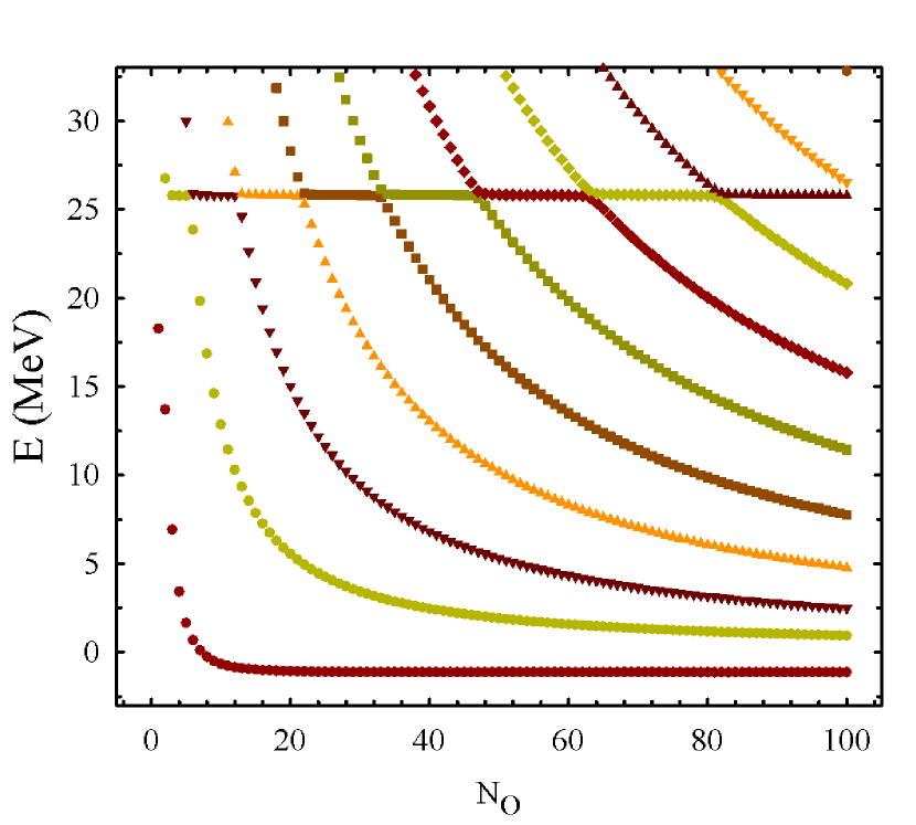
Figure 10: Spectrum of the 3/2^- states in ⁷Li as a function of the number of oscillator functions $N_{O}$ involved in calculations

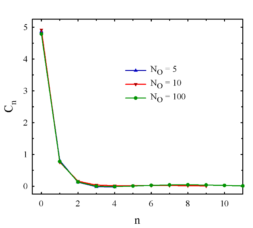
Figure 11: Convergence of wave function of the narrow 3/2^- Pauli resonance state in ⁷Li in the channel $\alpha+t$

III.4 Peculiarities of the Pauli resonance states

Let us consider peculiarities of the wave functions of the Pauli resonance state. Analysis of wave functions will allow us to understand nature of the Pauli resonances. Wave functions of resonance and nonresonant states are considered in the oscillator and coordinate representations.

In Fig. 12 we show three wave functions of the 3/2^- states in ⁷Li for clusterization $\alpha+t$. One of these functions is the wave function of the ground state (GS), the second function is the Pauli resonance state (PR) with energy $E$=25.810 MeV and the third function is the wave function of nonresonant, elastic $\alpha+t$ scattering state (SC) ($E$=10.1 MeV). Main difference between the Pauli resonance and nonresonant states wave functions is that the contribution of the oscillator function $\left|0\right\rangle$. This function gives the largest contribution to the wave function of the Pauli resonance states, and it has smallest contribution to the wave functions of the ground and continuous spectrum state.

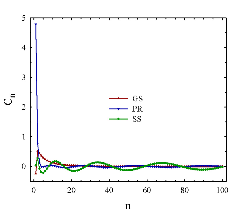
Figure 12: Wave functions in oscillator representation of the ground state (GS), Pauli resonance state (PR) and scattering state (SS) in the 3/2^- state of ⁷Li

In Fig. 13 we demonstrate wave functions of these states in coordinate space. As one should expect, nonresonant wave functions have a node at small distances ($r<$2.5 fm), while resonance wave function has the first node at relatively large distance ($r\approx$5.5fm). Besides, the resonance function has a very large amplitude, at list two times larger than the amplitude of the bound and scattering states.

Fig. 14 shows general picture of contribution of oscillator functions with the quantum numbers $n=0$ and $n=1$ to wave functions of continuous spectrum states over large energy range. Fig. 14 confirms also that the oscillator wave function with $n=0$ contribute mainly to the Pauli resonance state and gives a small contribution to other states of the $\alpha+t$ continuous spectrum.

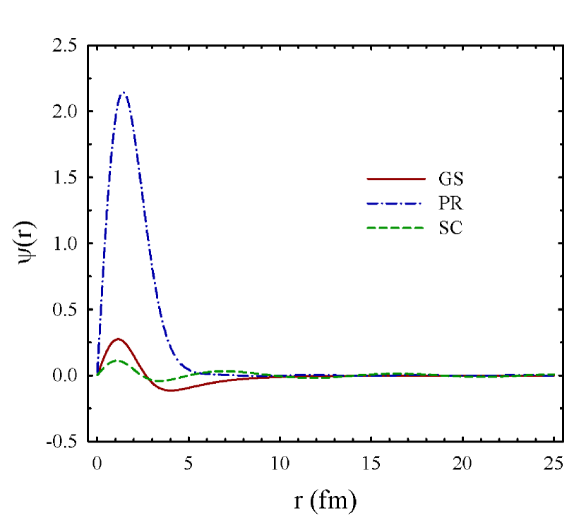
Figure 13: Wave functions of ⁷Li=$\alpha+t$ in coordinate space of the 3/2^- bound (BS), resonance (PR) and scattering (SC) states.

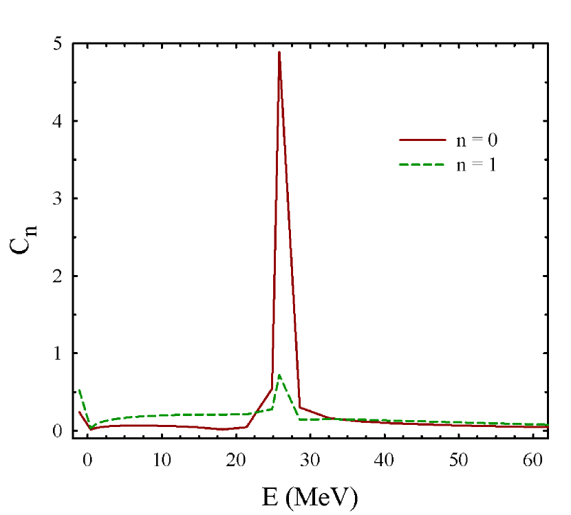
Figure 14: Contribution of the oscillator wave functions with $n=0$ and $n=1$ to wave functions of the continuous spectrum 3/2^- states of the $\alpha+t$ channel

Let us now consider a case with two Pauli resonance states. They are detected in the 1/2⁺ state of ⁷Li in the channel $\alpha+t$. Wave functions of two Pauli resonance states are shown in Fig. 15 in oscillator space and in Fig. 16 in coordinate space. Two oscillator functions with $n=0$ and $n=1$ give the main contribution to the Pauli resonance functions. As the results, these wave function in coordinate space describe a very compact two-cluster system, main part of which are concentrated at the small distances between clusters, namely $0\leq r\leq 5$ fm. Amplitudes of the wave functions in this small region are substantially larger than their amplitude at large distances.

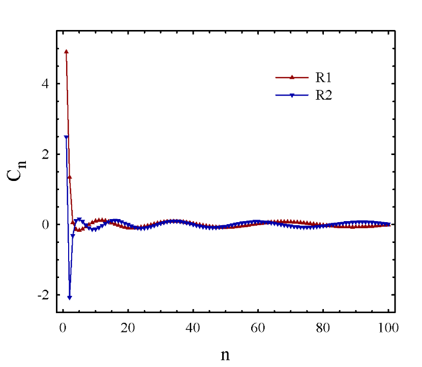
Figure 15: Wave functions in oscillator space of two Pauli resonance state in the 1/2⁺ state of ⁷Li

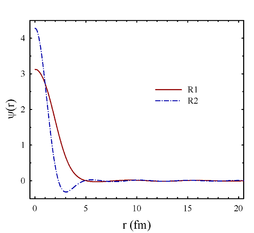
Figure 16: Wave functions in coordinate space of two Pauli resonances in the 1/2⁺ state in the $\alpha+t$ channel

III.5 Overlap

As it was widely recognized that mysteries (spurious) resonance states appear due to the Pauli principle, it is then expedient to analyze its effects on the norm kernels. Matrix of norm kernel in general case (for improved and advanced version of the RGM) is nondiagonal, thus we start the analysis with 3D picture of the matrix. In Fig. 17 we display the overlap matrix $\left\|\left\langle n|m\right\rangle\right\|$ for the channel $\alpha$+$t$ in the state $L$=0, $S$=1/2 and $J^{\pi}$=1/2⁺.  One can see that this matrix is a quasi-diagonal. The largest matrix elements are located on the main diagonal, and the larger is $m=n$, the close to unity they are. Off-diagonal matrix elements $\left\langle n|m\right\rangle$ are very small. A few diagonal matrix element with small values of $n$ are also small due to the Pauli principle. One may conclude that the Pauli principle has a short-range nature as it affects a relatively small number of cluster basis functions $\left|n\right\rangle$ (15) and corresponding matrix elements $\left\langle n|m\right\rangle$. Note that Fig. 17 demonstrates a typical behavior of matrix elements of norm kernel in the advanced version of the RGM for all nuclei and all states considered in this paper.

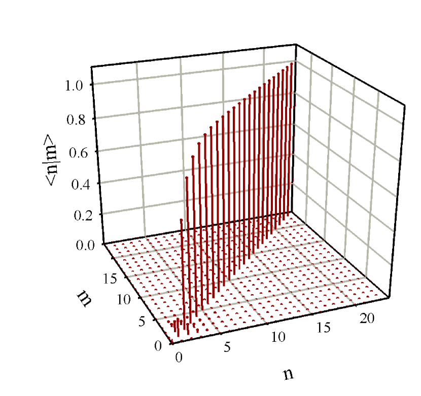
Figure 17: Matrix of norm kernel for the state $L$=0, $S$=1/2 and $J^{\pi}$=1/2⁺ of the channel $\alpha+t$

Fig. 17 prompts us to study only diagonal matrix elements of the norm kernel, which completely reflects effects of the Pauli principle. Consequently in this section we discuss the diagonal matrix elements and eigenvalues of the norm kernel. In Fig. 18 we compare diagonal matrix elements of the norm kernel, determined in the standard (S) and advanced (A) version of the RGM, for ⁷Li as two-cluster configuration $\alpha+t$. It is worthwhile recalling that in the standard version, the matrix of the norm kernel is diagonal. This figure demonstrates general features of the quantities $\left\langle n|n\right\rangle$ and $\Lambda_{\alpha}$ for all two-cluster systems under consideration. As was pointed our in previous paragraph, the major part of diagonal matrix elements are equal unity and only small fraction of them differ from unity, showing effects of the Pauli principle. It is necessary to recall that oscillator wave functions with small values of the quantum number $n$ describe two clusters at smallest relative distance, thus effects of the Pauli principle for these functions are prominent. One can see that there are two Pauli forbidden states in the 1/2⁺ state and one in the 3/2^- state within the standard version. In the advanced versions these basis states, namely, $\left|0\right\rangle$ and $\left|1\right\rangle$ for 1/2⁺ and $\left|0\right\rangle$ for 3/2^-, can be considered as almost-forbidden Pauli states, as the corresponding diagonal matrix elements are very small ($\left\langle n|n\right\rangle<0.1$). Fig. 18 demonstrates important features of matrix elements: the number of forbidden states in the standard version coincides with the number of almost-forbidden states in the advanced version.

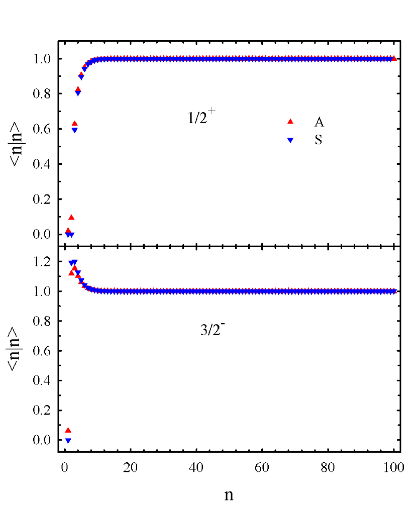
Figure 18: Comparison of diagonal matrix elements of the norm kernel, determined in the standard (S) and advanced (A) versions of the RGM for 1/2⁺ and 3/2^- states of ⁷Li=$\alpha+t$

The diagonal matrix elements $\left\langle n|n\right\rangle$ and eigenvalues $\Lambda_{\alpha}$ of the norm kernel for the $0^{+}$ and $1^{-}$ states of two-cluster system ⁶Li+$n$ are shown in Fig. 20. The almost forbidden states are found for the states $L^{\pi}=0^{+}$ and $S$=1/2 and $S$=3/2. Comparing Figs. 19 and 20 we see that the larger are interacting clusters, the larger is the region of diagonal matrix elements $\left\langle n|n\right\rangle$ which are affected of the Pauli principle.

In Fig. 19 we display the diagonal matrix elements $\left\langle n|n\right\rangle$ and eigenvalues $\Lambda_{\alpha}$ of the norm kernel for the $0^{+}$ states of cluster system ⁶Li+$d.$ Diagonal matrix element also show that there are a few almost forbidden states when $\left\langle n|n\right\rangle$ are close to zero. One may observe a set of the super-allowed Pauli states ($\left\langle n|n\right\rangle>1$) for the total spin $S$=1 and $S$=2. There are similarities between eigenvalues and the diagonal matrix elements of the norm kernel. The eigenvalues $\Lambda_{\alpha}$ reveals a few almost forbidden states, two states for $S$=1 and one state for the total spin $S$=0 and $S$=2. Similar to the diagonal matrix elements, the eigenvalues for $S$=0 and $S$=2 possess the super allowed states.

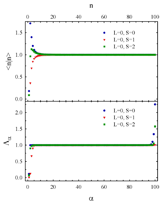
Figure 19: Diagonal matrix elements (the upper panel) and eigenvalues (the lower panel) of the norm kernel for the $L^{\pi}$= $0^{+}$ states and different values of the total spin $S$ in two-cluster system ⁶Li+$d$

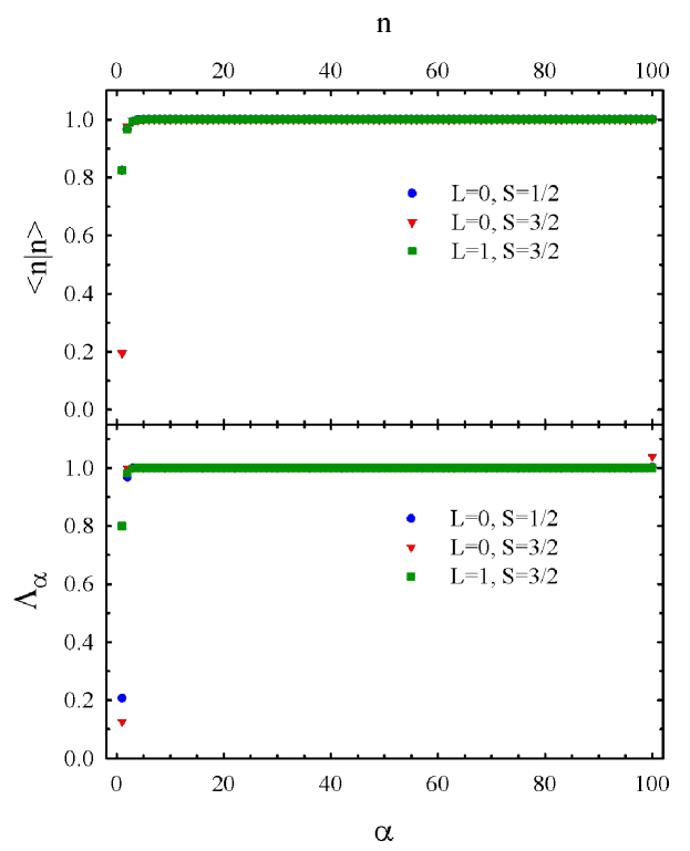
Figure 20: Diagonal matrix elements (the upper panel) and eigenvalues (the lower panel) of the norm kernel for two-cluster system ⁶Li+$n$.

Diagonal matrix elements $\left\langle n|n\right\rangle$ of the norm kernel and its eigenvalues $\Lambda_{\alpha}$ for the channel ⁶Li+$\alpha$ are displayed in Fig. 21. Two almost forbidden states are demonstrated by both diagonal matrix elements and eigenvalues. They are observed in two states: $L$=0, $S$=1, $J^{\pi}$=1⁺ and $L$=1, $S$=1, $J^{\pi}$=1^-.

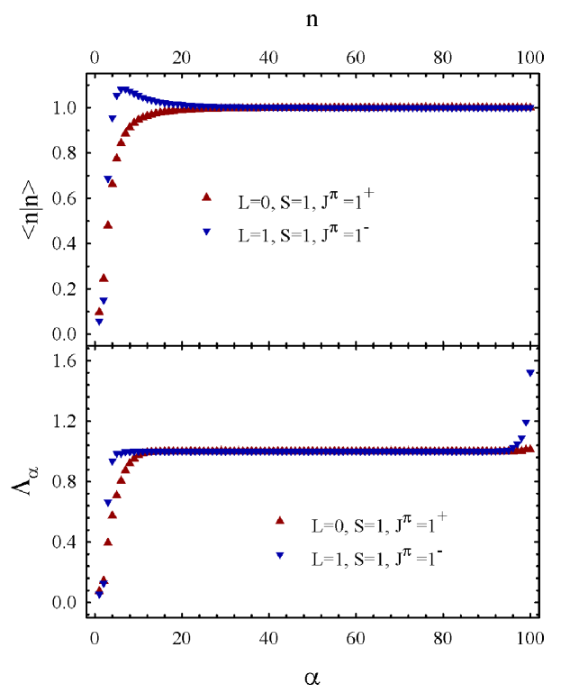
Figure 21: Diagonal matrix elements (upper panel) and eigenvalues (lower panel) of the norm kernel for the channel ⁶Li+$\alpha$ in the states $L$=0, $S$=1, $J^{\pi}$=1⁺ and $L$=1, $S$=1, $J^{\pi}$=1^-

Finishing this subsections, we conclude that the number of almost forbidden states coincides with the number of almost forbidden eigenstates. Almost forbidden states $\left|n\right\rangle$ obey the restriction $\left\langle n|n\right\rangle<0.3$, while almost forbidden eigenstates have $\Lambda_{\alpha}<0.2$. Comparing results demonstrated in Figs. 17, 18, 19, 20 with results of Tables 2 and 3 we came to the conclusion that the number of almost forbidden states equals of the number of the Pauli resonance states.

IV Method REV

Let us consider main ideas of the REV method formulated in Ref. Kruglanski and Baye (1992). The author of Ref. Kruglanski and Baye (1992) paid attention that a set of new eigenstates of the norm kernel appeared in the case when different oscillator lengths were used for an alpha particle and ¹⁶O. These eigenstates have very small values comparatively to eigenstates with the common oscillator length. For example, the smallest eigenvalue obtained for the total orbital momentum $L^{\pi}$=0⁺ with the common oscillator length is equal to 0.229, while there are four eigenstates with eigenvalues less than 0.03. Similar picture was also observed for the state $L^{\pi}$=1^-. The lowest eigenvalue obtained with the common oscillator length equals 0.344, for different oscillator lengths $b_{\alpha}$=1.395 fm and $b_{O}$=1.776 fm, four eigenstates emerged with eigenvalues less than 0.04.

It was suggested in Ref. Kruglanski and Baye (1992) to eliminate such eigenvalues and to use smaller set of norm kernel eigenstates. Thus in the case of different oscillator lengths, all eigenstates with eigenvalue smaller than eigenvalues with common oscillator length were treated as the Pauli forbidden states. Actually, the border between the Pauli allowed and Pauli forbidden state the Pauli allowed and Pauli forbidden states in system $\alpha+^{16}$O was selected to be 0.1. Having applied such restrictions, all Pauli resonance states disappeared.

We decided to use this method to eliminate the Pauli resonance states which appear in light nuclei within the advanced resonating group method. Analysis of the eigenvalues of the norm kernel carried out in Section III.5 indicates that we have to redetermine the border between the Pauli allowed and Pauli forbidden states.

Efficiency of the REV method will be demonstrated in Section V.1.

V Method ROF

We suggest another method to struggle with the Pauli resonance states in light nuclei. This method relay on properties of matrix elements of the norm kernel. By analyzing properties of the matrix elements, our attention was attracted by behavior of diagonal matrix elements $\left\langle n|n\right\rangle$. In many cases the matrix element $\left\langle 0|0\right\rangle$ and some times matrix element $\left\langle 1|1\right\rangle$ are very small with respect to other diagonal matrix elements. The analysis also revealed that matrix elements of corresponding row ($\left\langle 0|n\right\rangle$, $\left\langle 1|n\right\rangle$) and columns ($\left\langle n|0\right\rangle$, $\left\langle n|1\right\rangle$) are also very small. Besides, it was shown above (Section III.4) that oscillator functions with $n=0$ and sometimes with $n=1$ dominate in the wave function of the Pauli resonance states. Thus we suggest to omit those part of the matrix $\left\|\left\langle n|\widetilde{n}\right\rangle\right\|$ whose diagonal matrix elements are very small. We also suggest a criteria for smallness of the diagonal matrix elements. Let us introduce minimal value of the diagonal matrix elements $O_{\min}$ which will mark a border between the Pauli forbidden (or almost forbidden) and Pauli allowed states. Within our method, all diagonal matrix elements which are smaller than $O_{\min}$ will be omitted with their correspondent rows and columns.

Analysis of the diagonal matrix elements of the norm kernel leads us to the conclusion that in many two-cluster cases, considered above, $O_{\min}$ can be set to 0.2. This can be seen in Figs. 19, 20, 21. Such a value can be also used both for the case of one or two Pauli resonance states.

It is important to notice, that from mathematical point of view almost forbidden basis states or eigenstates are allowed states and should not create any problems. The same is true also from computational point of view, as the smallest eigenvalues are much larger than the smallest numerical value (numerical zero) in modern computers. Indeed, almost forbidden states do not create any problem for bound states and their parameters, such as root-mean-square mass and proton radii and so on. Presence of almost forbidden states affects (distorts) only continuous spectrum states. In this respect, both methods suggest re-determination of essentially allowed Pauli states. Both methods determine border between almost forbidden and allowed states. This border is marked by $\Lambda_{\min}$ and $O_{\min}$ in the REF and ROF  methods, respectively. In general case, one can use $\Lambda_{\min}$ and $O_{\min}$ as variational parameters to control the number of eliminated basis states $\left|n\right\rangle$ or eigenstates $\left|\alpha\right\rangle$ and their effects on scattering parameters. Naturally, the main aim of such procedure is to eliminate the Pauli resonance state(s) and to cause minimal effects on bound states and shape resonance states.

V.1 Demonstration of the REV and ROF methods

Having analyzed the diagonal matrix elements and eigenvalues of the overlap matrix, we deduced $O_{\min}$ and $\Lambda_{\min}$ for all nuclei and for those states $J^{\pi}$ which have the Pauli resonance states. These quantities are displayed in Table 4. In this table we also indicated the number $N_{f.s.}$ of eliminated basis functions or eigenfunctions.

Table 4: Actual values of $O_{\min}$ and $\Lambda_{\min}$, and the number of forbidden states $N_{f.s.}$, which are omitted to eliminate the Pauli resonance states

Nucleus	Clusterization	$L$	$S$	$J^{\pi}$	$O_{\min}$	$\Lambda_{\min}$	$N_{f.s}$
6Li	4He+$d$	0	1	$1^{+}$	0.2	0.2	1
		1	1	$2^{-}$	0.2	0.2	1
	3H+3He	0	1	$1^{+}$	0.1	0.1	1
		1	1	$2^{-}$	0.1	0.1	1
7Li	4He+3H	1	1/2	$3/2^{-}$	0.1	0.1	1
		1	1/2	$1/2^{-}$	0.1	0.1	1
		0	1/2	$1/2^{+}$	0.1	0.1	2
		2	1/2	$3/2^{+}$	0.1	0.1	1
	6Li+$n$	0	1/2	$1/2^{+}$	0.3	0.3	1
8Be	6Li+$d$	0	0	$0^{+}$	0.2	0.2	1
		0	1	$1^{+}$	0.1	0.1	1
		1	0	$1^{-}$	0.2	0.2	1
		1	1	$2^{-}$	0.3	0.3	1
		0	2	$2^{+}$	0.1	0.1	1
9Be	6Li+$t$	0	1/2	$1/2^{+}$	0.2	0.1	2
		1	1/2	$1/2^{-}$	0.1	0.1	1
		0	3/2	$3/2^{+}$	0.2	0.1	2
		1	3/2	$5/2^{-}$	0.1	0.1	1
		1	3/2	$5/2^{-}$	0.2	0.2	1
10B	6Li+4He	1	1	$0^{-}$	0.3	0.2	2
		1	1	$1^{-}$	0.3	0.2	2
		2	1	$1^{+}$	0.2	0.2	2
		2	1	$2^{+}$	0.2	0.2	1
		2	1	$3^{+}$	0.2	0.2	1

In Fig. 22 we demonstrate efficiency of the REV and ROF methods for the $\alpha+t$ scattering in the 1/2⁺ state. Here OA stands for ordinary algorithm of obtaining phase shifts within the advanced version of the RGM. The phase shift in this approach exhibits two Pauli resonance states, parameter of which are shown in Table 2. As we can see both methods remove the Pauli resonance states. They also yield the phase shifts which are close to the standard version at low energy region 0$\leq E<$6 MeV. There is very small difference of phase shifts obtained with the REV and ROF methods. We used minimal values of $\Lambda_{\min}=O_{\min}=0.2$. This restriction eliminated two functions in both methods.

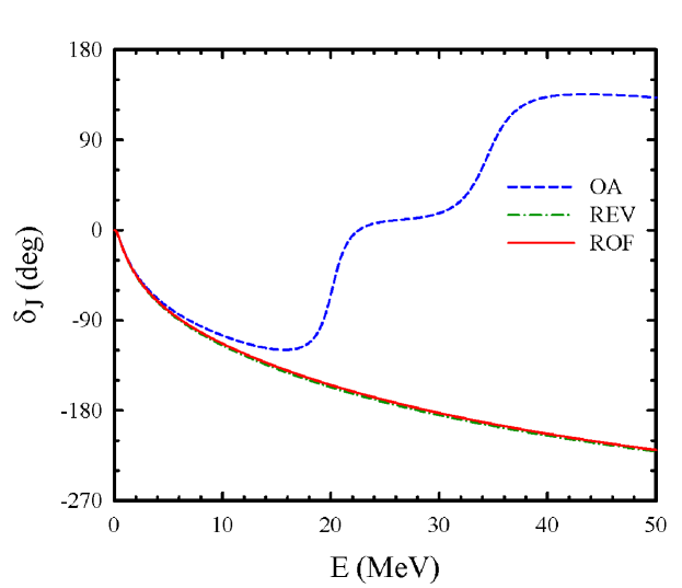
Figure 22: Phase shifts of the elastic $\alpha+t$ scattering in 1/2⁺ state as a function of energy determined in three different approaches.

The similar picture is observed for the $\alpha+d$ scattering in the 2^- state, see Fig. 23. Only one Pauli resonance state is generated in this case. Both REV and ROF methods remove that Pauli resonance state and produce the phase shifts with very small differences. In this case we also used minimal values of $\Lambda_{\min}=O_{\min}=0.2$. This restriction eliminated only one function in both methods.

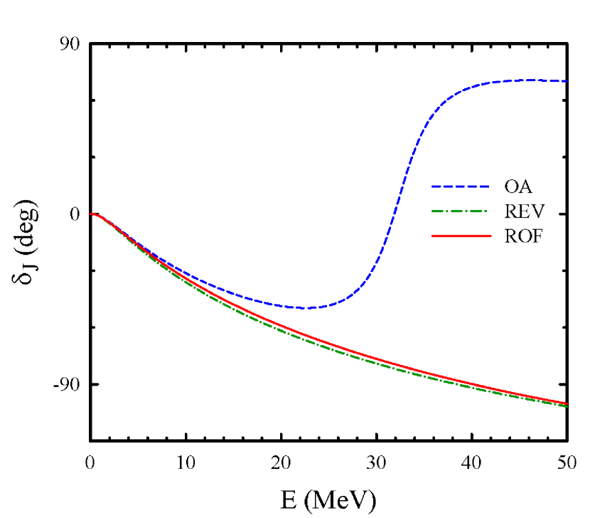
Figure 23: Phase shifts of the elastic $\alpha+d$ scattering in the 2^- state

Phase shifts of the elastic ⁶Li+$d$ scattering obtained within three different approaches are shown in Fig. 24. As one can see, in this case we observe both low-energy shape and high-energy Pauli resonance states. The REV and ROF methods eliminating one eigenfunction and one oscillator function, respectively, remove the Pauli resonance state. They also slightly change parameters of the shape resonance. In the original approach (OA) parameters of the shape resonance are $E$=0.153 MeV and $\Gamma$=0.013 MeV, while in the REV method they are $E$=0.374 MeV and $\Gamma$=0.485 MeV and in the ROF method we obtain $E$=0.352 MeV and $\Gamma$=0.371 MeV. Note that the REV and ROF give almost identical phase shifts of the ⁶Li+$d$ scattering. It means that the eliminated eigenfunction of the norm kernel and the eliminated oscillator function are close to each other.

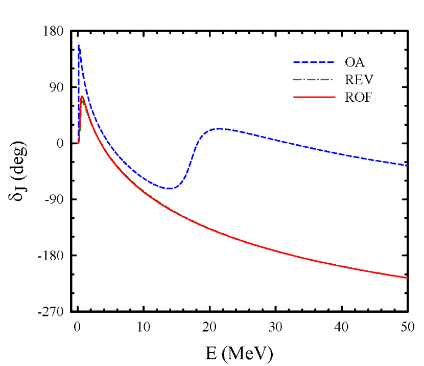
Figure 24: Phase shifts of the elastic ⁶Li+$d$ scattering in the state $L=0$, $S=0$ and $J^{\pi}=0^{+}$

We found several cases when the REV and ROF methods give noticeable different phase shifts. One of such examples is shown in Fig. 25, where phase shifts of the ⁶Li+$\alpha$ scattering in the state $L=1$, $S=1$ and $J^{\pi}=1^{-}$ are drawn. Note that almost the same results are observed for the state $J^{\pi}=0^{-}$ and $J^{\pi}=2^{-}$ generated by the coupling of the total orbital momentum $L=1$ with the total spin $S=1$. Two Pauli resonance states were removed by eliminating two eigenfunctions of the norm kernel obeying the restriction $\Lambda_{\alpha}\leq$0.2, and two oscillator functions with the restriction $\left\langle n|n\right\rangle\leq$0.3. Noticeable deviation of the phase shifts obtained in the REV and ROF methods is seen at the energy region $E>$3 MeV. Such deviation can be explained by structure of the eigenfunctions and their relation to oscillator functions. If an eigenfunction is mainly represented by one oscillator function, one may expect close results of both methods. If eigenfunction is spread over large number of oscillator functions, results obtained with these two method would be different. To prove this statement, we show in Fig. 27 eigenfunctions $\left\|U_{n}^{\alpha}\right\|$of the norm kernel as a function of $n$ for two different cases with two Pauli resonance states. We selected cases for elastic ⁶Li+$\alpha$ scattering with quantum numbers $L=S$=1, $J^{\pi}$=1^-and $L=0,$ $S$=1, $J^{\pi}$=1⁺. Phase shifts for them are shown in Figs 25 and 26. Fig. 27 demonstrates that for the $J^{\pi}$=1^- state, a large number of oscillator functions participate in formation of eigenfunctions $U_{n}^{1}$ and $U_{n}^{2}$. While for the $J^{\pi}$=1⁺ state, lowest oscillator functions with $n=0$ and $n=1$ totally dominates in corresponding eigenfunctions $U_{n}^{1}$ and $U_{n}^{2}$. Similar dominance of oscillator function with the quantum number $n=0$ in the eigenfunction $U_{n}^{1}$ are observed in all cases, when phase shifts obtained with the REV and ROF are coincide.

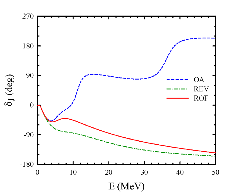
Figure 25: Phase shifts of the ⁶Li+$\alpha$ scattering in the state $L=1$, $S=1$, $J^{\pi}=1^{-}$ obtained with three different approaches.

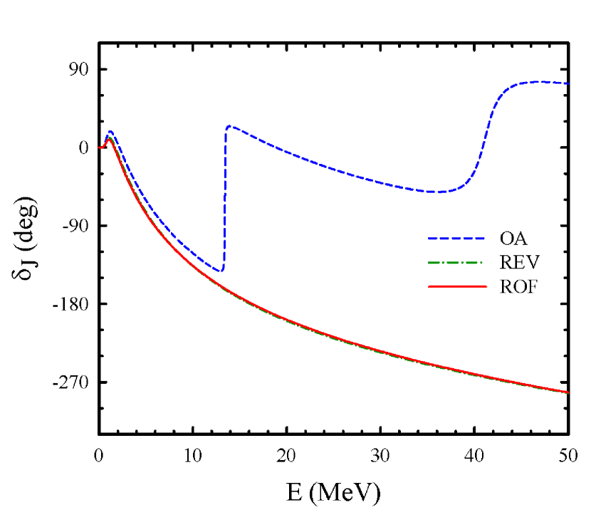
Figure 26: Phase shifts of the elastic ⁶Li+$\alpha$ scattering with J^π=1⁺ calculated within three approximations

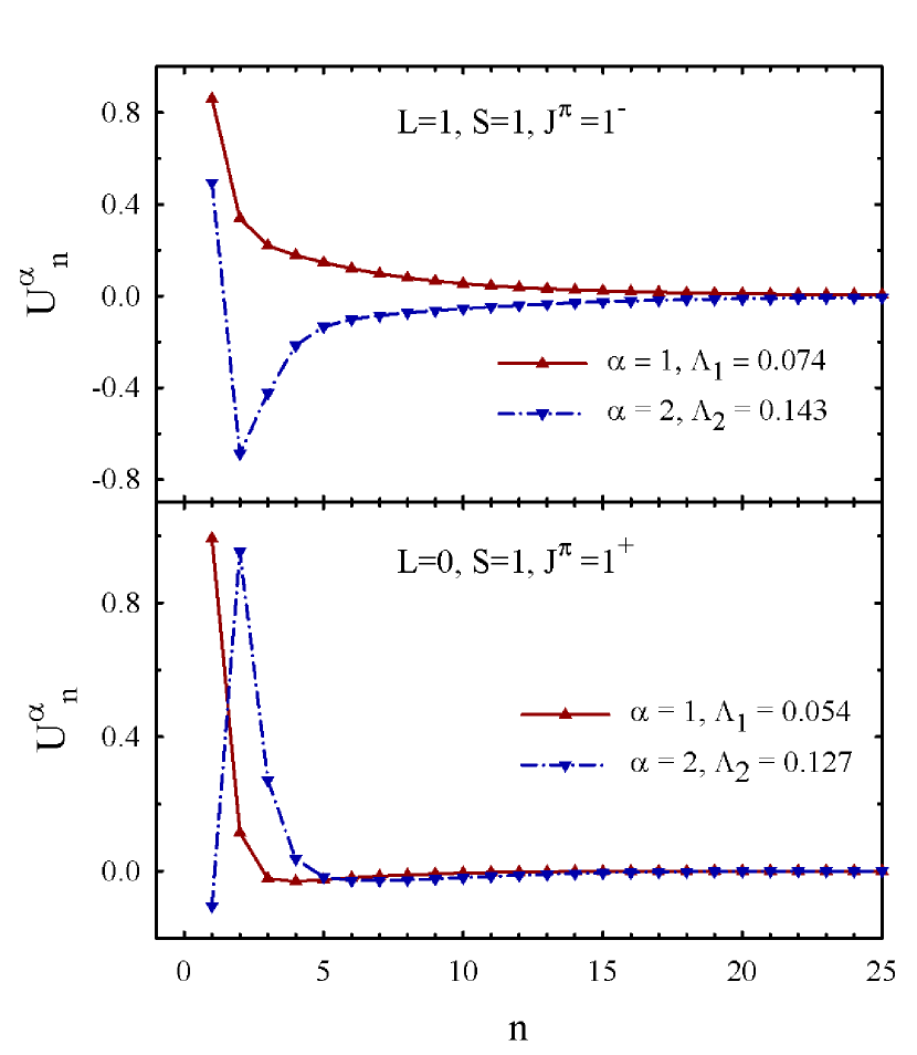
Figure 27: Eigenfunctions $U_{n}^{\alpha}$ of the norm kernel as a function of $n$ for $J^{\pi}$=1^- and $J^{\pi}$=1⁺ states in ¹⁰B, considered as two-cluster system ⁶Li+$\alpha$

In Table 5 we demonstrate effects of eliminated eigenfunctions and oscillator functions on parameters of bound and resonance states. These results are obtained for the 1⁺ states in ¹⁰B. By increasing $\Lambda_{\min}$ ($O_{\min})$ from zero to a certain value, indicated in the second column of Table 5, we manage to eliminate one two and three eigenfunctions (oscillator functions). In the fourth column of Table 28, we demonstrate how eliminated eigenfunctions and oscillator functions affect energy of the $1^{+}$ bound state of ¹⁰B. In Fig. 28 we show effects of eliminated functions on the ⁶Li+$\alpha$ phase shift. By eliminating one eigenfunction or one oscillator function, we remove the lowest Pauli resonance state and change position (lower down) of the second resonance on approximately 6.5 MeV. However, the energy of the ground state is slightly changed after removing one function. When we remove two eigenfunctions or two oscillator functions, both Pauli resonance states are disappeared. Two removed eigenfunctions increase energy of the bound state on 0.9 MeV, while two removed oscillator functions increase the energy on $\approx$1.3 MeV.

Table 5: Evolution of bound and resonance states in ¹⁰B. Energies and widths are in MeV

Method	$\Lambda_{\min}/O_{\min}$	$N_{f}$	$E_{GS}$	$E$	$\Gamma$	$E$	$\Gamma$
OA	0.0	100	-2.477	13.427	0.056	41.144	2.751
REV	0.1	99	-2.280	-	-	34.539	3.503
ROF	0.1	99	-2.264	-	-	34.826	3.684
REV	0.2	98	-1.527	-	-	-	-
ROF	0.2	98	-1.183	-	-	-	-
REV	0.7	97	-0.132	-	-	-	-
ROF	0.7	97	0.526	-	-	-	-

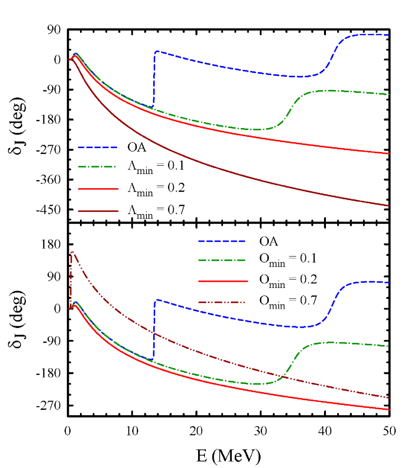
Figure 28: Phase shifts of the elastic ⁶Li+$\alpha$ scattering obtained with different values of $\Lambda_{\min}$ (the upper part) and $O_{\min}$ (the lower part)

As we pointed out above, oscillator functions with small values of the quantum number $n$ and eigenfunctions with small value of index $\alpha$ describe the most compact two-cluster configurations. It is interesting to analyze effects of their deletion on energies of bound states and shape resonances, if they appear. For this aim we collected in Table 6 energies of bound and resonance states.

Table 6: Effects of removed eigenfunctions and oscillator functions on energy of bound and shape resonance states

Nucleus	Channel	$J^{\pi}$	Parameter	OA	REV	ROF
7Li	$\alpha+t$	3/2-	$N_{f}$	100	99	99
			$E_{GS}$, MeV	-1.127	-1.105	-1.064
8Be	6Li$+d$	0+	$N_{f}$	100	99	99
			$E_{GS}$, MeV	-18.971	-15.281	-14.426
			$E$, MeV	0.153	0.374	0.352
			$\Gamma$, MeV	0.013	0.485	0.371
		2-	$N_{f}$	100	99	99
			$E$, MeV	0.800	0.825	0.805
			$\Gamma$, MeV	0.738	0.957	0.762
10B	6Li$+\alpha$	1+	$N_{f}$	100	98	98
			$E_{GS}$, MeV	-2.477	-1.527	-1.183

V.1.1 Preliminary conclusions

At the end of this section we made preliminary conclusions concerning the REV and ROF methods. In all cases, presented above, both methods completely remove all detected Pauli resonance states. In many cases, both methods give close results for phase shifts. In some cases, phase shifts are somewhat different. Such a difference as we demonstrated, appear when eigenfunctions of the norm kernel are spread over a large number of oscillator functions. In other words, removed eigenfunctions and removed oscillator functions are quit different. When results of both method coincide, removed eigenfunctions are presented mainly by removed oscillator functions.

We demonstrated that the ROF method, formulated in this paper, is an alternative method to the one suggested by Kruglanski and Baye. Advantage of the ROF is that it does no require an orthogonalization procedure of matrices of norm kernel and then transformation of matrix of Hamiltonian to new representation. This procedure is time consuming when a large number of basis functions are involved. We also demonstrated that oscillator representation is appropriate tool for studying effects of the Pauli principle on kinematic (matrix of norm kernel) and dynamics (matrix of Hamiltonian) of two- and many-cluster systems.

VI Conclusions

Properties of Pauli resonance states in two-body continuum of the light nuclei ⁶Li, ⁷Li, ⁷Be, ⁹Be and ¹⁰B have investigated within the advanced version of the resonating group method. The advanced version employs a three-cluster configuration which allows to consider in general case three two-body (binary) channels. One of constituents of a binary channel is considered as a two-cluster subsystem, which provides us with more correct description of the nuclei having distinct two-cluster structure and a small separation energy. Wave functions of two-cluster subsystem are obtained by solving appropriate Schrödinger equation. The advanced version we have employed make use of the square-integrable bases - Gaussian and oscillator bases. Gaussian basis is used to describe relative motion of two clusters in two-cluster subsystem and is very efficient in obtaining wave functions of bound states with minimal number of basis functions. Oscillator basis is used to study interaction of the third cluster with two-cluster subsystem. It allows us to implement proper boundary condition for discrete and continuous spectrum states. It was demonstrated that oscillator basis is suitable tool to study effects of the Pauli principle and to reveal nature of the Pauli resonance states.

It was demonstrated that the advanced form of two-cluster subsystem is the origin of the Pauli resonance states. More precisely, an advanced form of wave function of two-cluster subsystem is responsible for appearance of the Pauli resonance states.

It has been shown that the Pauli resonance states appear at the relatively high energy $E>$11 MeV. Some of these resonance states are very narrow resonance states, however, major part of them are broad resonance states. The most populated area of resonance states lies in the interval 16$<E<$21 MeV. Two dense area of widths of resonance states are located in intervals 0.008$<\Gamma<$0.22 MeV and 0.9$<\Gamma<$1.2 MeV.

It was found that the oscillator functions with minimal value of the quantum number $n$ (the number of radial oscillator quanta) dominates in resonance wave functions. These basis functions yields very small values of the diagonal matrix elements $\left\langle n|n\right\rangle$ of the norm kernel. It was also demonstrated that the very narrow Pauli resonance states can be detected by using a very small number of oscillator functions: from three to five functions.

We have established that the Pauli principle predetermine appearance of the Pauli resonance states by creating almost forbidden states, however energies and widths of the Pauli resonance states are mainly formed by nucleon-nucleon forces.

We found that the number of Pauli resonance states for the given $J^{\pi}$ state, discovered within the advanced version of the RGM, coincides with the number of the Pauli forbidden states determined in the standard version of the RGM.

One of the main conclusions of the present paper is that one needs to find proper definition of the Pauli forbidden and Pauli allowed (fully or partially) states. Standard or formal definition for Pauli forbidden states is that the eigenvalues for them should be equal zero $\Lambda_{\alpha}=0$. Then, the Pauli allowed states should have $\Lambda_{\alpha}>0$. However, the carried out analysis leads us to the conclusion that for light nuclei with two-body clusterization the border between forbidden and allowed states is $\Lambda_{\min}=0.2$. It was also shown that oscillator functions $\left|n\right\rangle$ which generates diagonal matrix elements of the norm kernel $\left\langle n|n\right\rangle\leq O_{\min}=0.2$, can be considered as the Pauli forbidden states. By removing of the Pauli forbidden states, one eliminates the Pauli resonance states and causes minor effects on energy of bound states and energy and width of the shape resonance states, if they exist. We have not found universal values of $\Lambda_{\min}$ and $O_{\min}$ for all light nuclei, which have been considered.

As for perspective of this work. In the present paper we have restricted ourselves to a single-channel approximation to reveal the Pauli resonance states and find main factors responsible for formation of such states. In the future we are planning to consider appearance of the Pauli resonance states in many-channel systems and how the REF and ROF can help to eliminate them. Many-channel cases are specially interesting since small eigenvalues of the norm kernel can appear due to strong overlap of basis functions belonging to different channels. This strong coupling is not directly related to the Pauli principle. This makes the problem more attractive and challenging.