S1 Box and Residual Computation

We provide details of $\ominus,\oplus$ computation between boxes and residuals. Conventional 3D object detectors represent 3D boxes with 7-dimensional vectors $(x,y,z,w,h,l,\theta)$. Here, $(x,y,z)$ represents center coordinates of boxes, $(w,h,l)$ represents sizes of boxes, and $\theta$ represents yaw rotation along the z-axis. According to box encoding function (second_yan), residual $x^{gt}$ between proposal box $X^{P}$ and target object box $X^{T}$ is formulated as follows:

$$x^{gt} =X^{P}\ominus X^{T}$$

$$=(\Delta x,\Delta y,\Delta z,\Delta w,\Delta h,\Delta l,\Delta\theta),$$ (S1)

$$\Delta x =\frac{x^{T}-x^{P}}{d^{P}},\Delta y=\frac{y^{T}-y^{P}}{d^{P}},\Delta z=\frac{z^{T}-z^{P}}{h^{P}},$$ (S2)

$$\Delta w =\mathrm{log}(\frac{w^{T}}{w^{P}}),\Delta h=\mathrm{log}(\frac{h^{T}}{h^{P}}),\Delta l=\mathrm{log}(\frac{l^{T}}{l^{P}}),$$ (S3)

$$\Delta\theta =\theta^{T}-\theta^{P}.$$ (S4)

Here, $d^{P}=\sqrt{(w^{P})^{2}+(h^{P})^{2}}$ is the diagonal of the base of the box, the superscripts $P$ and $T$ indicate the proposal and target, respectively. Above formulation is expressed as $x^{gt}=X^{T}\ominus X^{P}$ for brevity. In contrast, $\oplus$ represents box transformation by residual, which is inverse of $\ominus$.

S2 Residual Normalization

DiffRef3D samples noise from Gaussian distribution $\mathcal{N}(0,I)$ to generate noisy residuals. However, directly applying sampled noises as box residuals would result in unlikely hypotheses since residuals in 3D object detection have a different distribution. From our observation of the true residual distribution, we propose to adaptively normalize the residuals with respect to the shape and size of the proposal. Accordingly, we formulate box normalization using the notations above as follows:

$$x^{gt}_{norm}=(\frac{\Delta x}{d^{P}},\frac{\Delta y}{d^{P}},\frac{\Delta z}{l^{P}},\frac{\Delta w}{d^{P}},\frac{\Delta h}{d^{P}},\frac{\Delta l}{l^{P}},\frac{\Delta\theta}{r^{P}})$$ (S5)

Here, $r^{P}=\mathrm{max}(w^{P}/h^{P},h^{P}/w^{P})$ is the aspect ratio of the base of the proposal.

S3 Training Losses

For two-stage 3D object detectors, the first stage region proposal network (RPN) and the second stage proposal refinement module are trained with independent training losses, respectively. As the main contribution of DiffRef3D lies on the second stage, we provide the details of training losses for our proposal refinement module here. DIffRef3D-V, PV, and T adopts the same training losses of the respective baselines. For all three models, the classification loss $L_{cls}$ and the regression loss $L_{reg}$ is employed to supervise the confidence and bounding box prediction $\hat{c}$ and $\hat{x}$, respectively.

For regression loss $L_{reg}$, the smooth-L1 loss is computed in two terms: residuals and box corner points. It is formulated as follows:

$$L_{reg}=\mathbb{1}(\mathrm{IoU}_{i}\geq\theta_{reg})\frac{1}{N_{P}}\sum^{N_{P}}_{i=1}[\mathrm{smoothL1}(x^{gt}_{i},\hat{x}^{(t)}_{i})\\ +\sum^{8}_{j=1}\mathrm{smoothL1}(b^{T}_{i,j},b^{P}_{i,j})].$$ (S6)

$\mathrm{IoU}_{i}$ represents $\mathrm{IoU}$ between $i$-th proposal and corresponding target box and $\mathbb{1}(\mathrm{IoU}_{i}\geq\theta_{reg})$ indicates that only region proposals with $\mathrm{IoU}$ over threshold $\theta_{reg}$ contributes to the regression loss, $N_{P}$ is number of proposals. For corner loss, $b_{i,j}$ indicates $j$-th corner point coordinates, and superscripts $T$ and $P$ indicate the target object box and proposal box, respectively.

In case of classification loss $L_{cls}$, the target is assigned by an $\mathrm{IoU}$ related value. Specifically, the target for $i$-th proposal is assigned as follows:

$$c^{gt}_{i}=\begin{cases}1&\mathrm{IoU}_{i}\geq\theta_{H},\\ \frac{\mathrm{IoU}_{i}-\theta_{L}}{\theta_{H}-\theta_{L}}&\theta_{L}\leq\mathrm{IoU}_{i}<\theta_{H},\\ 0&\mathrm{IoU}_{i}<\theta_{L},\end{cases}$$ (S7)

and the binary cross-entropy loss is computed according to assigned target as follows:

$$L_{cls}=\frac{1}{N_{P}}\sum^{N_{P}}_{i=1}L_{BCE}(c^{gt}_{i},\hat{c}_{i}).$$ (S8)

DiffRef3D-PV employs additional keypoint segmentation loss (pvrcnn_shi) to the above losses, which is implemented with a Focal loss (focal_yun) supervised with the foreground label for each keypoint. Formally, the segmentation loss $L_{seg}$ is formulated as:

$$L_{seg}=-\frac{1}{N_{kp}}\sum^{N_{kp}}_{k=1}L_{Focal}(s_{k}^{gt},\hat{s}_{k})$$ (S9)

where $N_{kp}$ is the number of keypoints, $\hat{s}_{k}$ denotes the foreground score prediction. The foreground label $s^{gt}_{k}$ is assigned as 1 if the keypoint lies inside an object bounding box, otherwise 0.

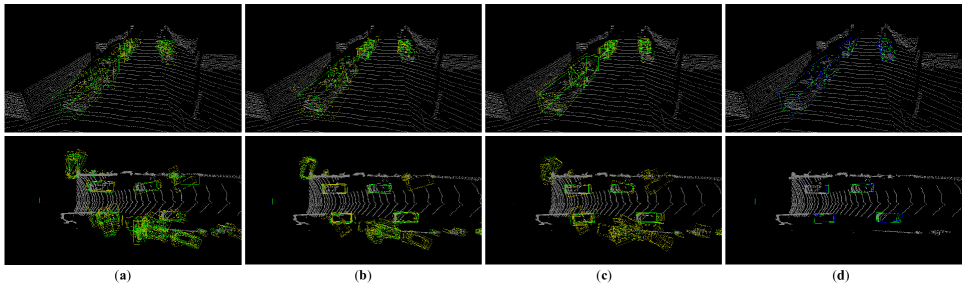
Figure S1: More qualitative results. Visualizations of iterative sampling steps of DiffRef3D on various scenes. Each image shows hypotheses and predictions at (a) t=1000, (b) t=500, (c) t=200, and (d) the final prediction. Hypotheses are colored in yellow, predictions are colored in green, and ground truths are colored in blue.

S4 Additional Experiments

Figure S2: Hypotheses generation on different SNRs. We visualize how hypotheses are generated based on reference boxes according to various SNRs at timestep $t=1000$. Hypotheses are colored in yellow, reference boxes are colored in green.

In this section, we present more qualitative results and ablation studies on the KITTI benchmark (kitti). Figure S1 shows visualization results on the inference phase in various scenes.

Signal-to-Noise Ratio

Table S1: Ablation studies with different signal-to-noise ratio on the KITTI val set with AP (R40) for moderate difficulty.

SNR	Car		Pedestrian		Cyclist
	step1	step3	step1	step3	step1	step3
1	77.80	77.89	61.36	62.83	68.63	69.44
2	84.98	84.77	60.45	63.07	71.80	74.20
4	83.47	83.47	62.47	63.44	71.57	72.39

We further study the influence of signal-to-noise ratio (SNR) in Table S1. Results demonstrate that the SNR of 2 achieves optimal AP performance on the KITTI val set. We explain that performance degradation at SNR of 1 is due to impractical shapes of hypotheses that fall short on detection. Figure S2 illustrates how hypotheses are generated based on proposals according to each SNR. Hypotheses generated by SNR of 1 could appear far from proposal which leverages irrelevant features, and SNR of 4 generates hypotheses condensed on proposals which lack to exploit additional local features. Note that, Table S1 highlights AP improvements at larger sampling steps in general regardless of SNR, which implies the effectiveness of iterative sampling steps by the diffusion process on 3D object detection.

Attention Mechanism

Table S2: Ablation studies with different implementation of attention mechanism on the KITTI val set with AP (R40) for moderate difficulty. Method ”MLP” stands for employing a multi-layer perceptron rather than the attention block, ”C.A.” stands for the cross-attention between proposal and hypothesis feature, and ”S.A.” stands for the self-attention on hypothesis feature, respectively. Involving $x_{t}$ indicates embedding positional information from noisy residuals into features or queries.

Method	Involve	Mod. AP(R40), step3
	$x_{t}$	Car	Ped.	Cyc.
MLP		82.37	62.23	72.28
	✓	82.48	61.49	73.68
C.A.		82.56	62.66	72.52
	✓	82.82	63.81	72.79
S.A.		83.44	64.62	72.92
	✓	84.77	63.07	74.20

We conduct experiments to further verify design choice of attention mechanism in hypothesis attention module (HAM). Table S2 demonstrates results of various implementations, on the KITTI val set with sampling steps of 3. Only with self-attention already outperforms other methods involving $x_{t}$ on every class, and AP gains derived from involving $x_{t}$ is higher at self-attention compared to other methods. Therefore, we designed our HAM to include a self-attention block involving $x_{t}$ as positional embedding on query.

Temporal Transformation Block

As shown in Fig. S1, hypotheses generated at smaller timestep are located closer to the predicted object bounding box. Figure 4 in the main manuscript also highlights that our temporal transformation block regularizes the contribution of the hypothesis feature with respect to timestep. Table S3 quantitatively presents the effect of the temporal transformation block, verifying its necessity.

Table S3: Ablation studies with temporal transformation block on the KITTI val set with AP (R40) for moderate difficulty.

TT	Car		Pedestrian		Cyclist
	step1	step3	step1	step3	step1	step3
	77.80	77.89	61.36	62.83	68.63	69.44
✓	84.98	84.77	60.45	63.07	71.80	74.20

Table S4: Ablation studies with box ensemble methods on the KITTI val set with AP (R40) for moderate difficulty pedestrian class. Method ”None” stands for no ensemble applied during the iterative sampling steps, ”NMS” stands for the non-maximum suppression applied on ensemble of box predictions then applied averaging, and ”Mean” stands for the averaging ensemble of box predictions, respectively.

Ensemble	Sampling Steps
	1	2	3
None	60.45	62.70	61.13
NMS	60.45	60.58	60.56
Mean	60.45	62.77	63.07

Box Ensemble

We further compare the box ensemble methods during the inference phase. Table S4 summarizes the comparison results. Notably, non-maximum suppression (NMS) results lower AP (R40) compared to no ensemble applied. Box ensemble via averaging outperforms other methods along each sampling step, thus we adopted the method to boost detection performance.