SMURF-THP: Score Matching-based UnceRtainty quantiFication for Transformer Hawkes Process

Abstract

Transformer Hawkes process models have shown to be successful in modeling event sequence data. However, most of the existing training methods rely on maximizing the likelihood of event sequences, which involves calculating some intractable integral. Moreover, the existing methods fail to provide uncertainty quantification for model predictions, e.g., confidence intervals for the predicted event’s arrival time. To address these issues, we propose SMURF-THP, a score-based method for learning Transformer Hawkes process and quantifying prediction uncertainty. Specifically, SMURF-THP learns the score function of events’ arrival time based on a score-matching objective that avoids the intractable computation. With such a learned score function, we can sample arrival time of events from the predictive distribution. This naturally allows for the quantification of uncertainty by computing confidence intervals over the generated samples. We conduct extensive experiments in both event type prediction and uncertainty quantification of arrival time. In all the experiments, SMURF-THP outperforms existing likelihood-based methods in confidence calibration while exhibiting comparable prediction accuracy.

1 Introduction

Sequences of discrete events in continuous time are routinely generated in many domains such as social media (Yang et al.,, 2011), financial transactions (Bacry et al.,, 2015), and personalized treatments (Wang et al.,, 2018). A common question to ask is: Given the observations of the past events, when and what type of event will happen next? Temporal point process such as the Hawkes process (Hawkes,, 1971) uses an intensity function to model the arrival time of events. A conventional Hawkes process defines a parametric form of the intensity function, which assumes that the influence of past events on the current event decreases over time. Such a simplified assumption limits the model’s expressivity and fails to capture complex dynamics in modern intricate datasets. Recently, neural Hawkes process models parameterize the intensity function using recurrent neural networks (Du et al.,, 2016; Mei and Eisner,, 2017) and Transformer (Zuo et al.,, 2020; Zhang et al.,, 2020). These models have shown to be successful in capturing complicated event dependencies.

However, there are two major drawbacks with existing training methods for neural Hawkes process models. First, they mainly focus on maximizing the log-likelihood of the events’ arrival time and types. To calculate such likelihood, we need to compute the integral of the intensity function over time, which is usually computationally challenging, and therefore numerical approximations are often applied. As a result, not only is the computation complex, but the estimation of the intensity function can still be inaccurate in these likelihood-based methods. Second, the arrival time of events often follows a long tail distribution, such that point estimates of the arrival time are unreliable and insufficient. Thus, confidence intervals that can quantify model uncertainty are necessary. However, calculating the confidence interval directly from density is computationally challenging. This is because we need to compute the coverage probability, which is essentially another integral of the intensity function (recall that the intensity is an infinitesimal probability).

To overcome the above two challenges, we propose SMURF-THP, a score-based method for learning Transformer Hawkes process models and quantifying the uncertainty of the models’ predicted arrival time. The score-based objective in SMURF-THP, originally introduced by Hyvärinen and Dayan, (2005), is to match the derivative of the log-likelihood (known as score) of the observed events’ arrival time to the derivative of the log-density of the empirical (unknown) distribution. Note that calculating scores no longer requires computing the intractable integral in the likelihood function. Moreover, SMURF-THP is essentially a score-based generative model: With the neural score function learnt by SMURF-THP, we can generate samples from the predicted distribution of the arrival time. This naturally allows for the quantification of uncertainty in predictions by computing confidence intervals over the generated samples.

Note that Transformer Hawkes process jointly models event types and arrival time. Because score matching methods can only be applied to handle the continuous arrival time but not the categorical event types, we need to decompose the joint likelihood into a marginal likelihood of the arrival time and a partial likelihood of the types. When training the Transformer Hawkes process models using SMURF-THP, the objective becomes a weighted sum of the score-matching loss (which replaces the marginal likelihood of the arrival time) and the negative partial log-likelihood of event types.

We demonstrate the effectiveness of SMURF-THP for learning Transformer Hawkes process models on four real-world datasets, each of which contains sequences of multiple types of discrete events in continuous time. We decompose the joint likelihood by conditioning event type on the arrival time and consider a Transformer Hawkes process where one single intensity function is shared across all event types. Our experimental results show that compared with likelihood-based methods, SMURF-THP demonstrates superior performance on uncertainty quantification of arrival time, while exhibiting comparable event-type prediction accuracy. For example, SMURF-THP achieves within 0.3% prediction accuracy compared with likelihood-based methods, while gaining 4-10% confidence calibration in predictions of arrival times.

The rest of the paper is organized as follows: Section 2 briefly reviews the background, Section 3 describes our proposed method, Section 4 presents the experimental results, and Section 5 discusses the related work and draws a brief conclusion.

2 Background

We briefly review the neural Hawkes process models, the Transformer model and the score matching method.

2.1 Neural Hawkes Process

For simplicity, we review neural Hawkes process with only one event type. And we will introduce Hawkes process with multiple event types (i.e., marked point process) in the next section. Let $\mathcal{S}=\{t_{i}\}_{i=1}^{L}$ denote an event sequence with length $L$, where each event is observed at time $t_{i}\in[0,t_{\max}]$. We further denote the history up to time $t$ as $\mathcal{H}_{t}=\{t_{j}:t_{j}<t\}$, and the conditional intensity function as $\lambda(t\mid\mathcal{H}_{t})$. Then, we have the conditional probability of the next event proceeding $t_{i-1}$ as:

$$p_{T}(t\mid\mathcal{H}_{t_{i}})=\lambda(t\mid\mathcal{H}_{t_{i}})e^{-\int_{t_{i-1}}^{t}\lambda(\tau\mid\mathcal{H}_{t_{i}})d\tau}.$$ (1)

The log-likelihood of the event sequence $\mathcal{S}$ is then

$$\ell_{0}(\mathcal{S})=\sum_{i=1}^{L}\log\lambda(t_{i}|\mathcal{H}_{t_{i}})-\int_{0}^{t_{\max}}\lambda(\tau|\mathcal{H}_{t_{i}})d\tau.$$ (2)

Notice that exact computation of the integral in Eq. (1) is intractable, such that numerical approximations are required.

Neural Hawkes Process parameterizes the intensity function $\lambda$ with deep neural networks. For example, Du et al., (2016); Mei and Eisner, (2017) use variants of recurrent neural networks, and Zuo et al., (2020); Zhang et al., (2020) use the Transformer model (Vaswani et al.,, 2017). Other examples include employments of deep Fourier kernel (Zhu et al.,, 2021) and feed-forward neural networks (Omi et al.,, 2019).

2.2 Transformer Model

In this paper, we parameterize the intensity function $\lambda$ in Eq. (1) using a Transformer model (Vaswani et al.,, 2017). The Transformer model has multiple Transformer layers, where each layer contains a self-attention mechanism and a feed-forward neural network. The self-attention mechanism assigns attention weights to every pair of events in a sequence. These weights signify the strength of the dependency between pairs of events, with smaller weights indicating weaker dependencies and larger weights suggesting stronger ones. Such mechanism efficiently models the dependencies between events irrespective of their position in the sequence, thereby capturing long-term effects. The feed-forward neural network in each layer further incorporates non-linearities to offer a larger model capacity for learning complex patterns. Studies have shown that the Transformer model outperforms recurrent neural networks in modeling event sequences (Zuo et al.,, 2020; Zhang et al.,, 2020).

2.3 Score Matching

Score matching (Hyvärinen,, 2005) is originally designed for estimating non-normalized statistical methods on $\mathbb{R}^{n}$ without challenging computation of the normalization term. In practice, however, score matching is not scalable to high-dimensional data and deep neural networks due to the calculation of derivative of density. Denoising score matching (Vincent,, 2011) is one of its variants that circumvent the derivative by adding perturbation to data points. Song et al., (2019) also enhance the scalability by projecting the score function onto random vectors. Yu et al., (2019) and Yu et al., (2022) further generalize the origin score matching to accommodate densities supported on a more general class of domains. Early work (Sahani et al.,, 2016) has adopted score matching in modeling Poisson point process, but it fails to model complicated event dependencies induced in the modern event data due to the simplified assumption that the intensity function is independent of the historical events. A suitable sampling algorithm for score matching-based models is Langevin Dynamics (LD), which can produce samples from a probability density using only its score function. Hsieh et al., (2018) propose Mirror Langevin Dynamics (MLD) as a variant of Langevin Dynamics that focuses on sampling from a constrained domain. We employs both LD and MLD for generating event samples in our experiments.

3 Method

3.1 Score Matching Objective of Hawkes Process

Let $\mathcal{S}=\{(t_{i},k_{i})\}_{i=1}^{L}$ denote an event sequence of length $L$, where each pair $(t_{i},k_{i})$ corresponds to an event of type $k_{i}\in\{1,\cdots,M\}$ happened at time $t_{i}\in[0,t_{\mathrm{max}}]$. Also, we denote the history events up to time $t$ as $\mathcal{H}_{t}=\{(t_{j},k_{j}):t_{j}<t\}$. Our goal is to learn $p_{T,K}(t,k{\,|\,}\mathcal{H}_{t})$, the joint conditional probability of the event proceeding time $t$ given the history $\mathcal{H}_{t}$.

To employ score matching, we decompose the joint conditional pdf $p_{T,K}$ by conditioning on the event time. By doing so, the partial likelihood of the discrete event types can be maximized by minimizing the cross entropy loss; and the marginal likelihood of the continuous event time can be substituted by a score-matching objective. Such a substitution avoids the intractable integral of the intensity. Specifically, we condition $p_{T,K}$ on the event time and we have:

$$p_{{T,K}}(t,k{\,|\,}\mathcal{H}_{t})=p_{T}(t{\,|\,}\mathcal{H}_{t})\cdot p_{{K{\,|\,}T}}(k{\,|\,}t,\mathcal{H}_{t}).$$ (3)

Correspondingly, we have the log-likelihood:

$$\ell(\mathcal{S})\!=\!\sum_{i=1}^{L}\log p_{T}(t_{i}|\mathcal{H}_{t_{i}})\!+\!\sum_{i=1}^{L}\log p_{{K|T}}(k_{i}|t_{i},\mathcal{H}_{t_{i}}).$$ (4)

We can use a neural network to parameterize the intensity function and directly train the model using Eq. (4). However, such an approach inevitably faces computational challenges, i.e., exact computation of the intensity’s integral is intractable. Therefore, we derive a score-matching objective to substitute the first term in Eq. (4).

In SMURF-THP, we use a Transformer model with parameters $\theta$ to parameterize the intensity function. More details are presented in Section 3.3. A sample’s score is defined as the gradient of its log-density. Then, using Eq. (1), we can write the score of the $i$-th event given its history $\mathcal{H}_{t_{i}}$ and the model parameters $\theta$ as:

$${\psi}(t_{i}{\,|\,}\mathcal{H}_{t_{i}};\theta)=\partial_{t}\log{p_{T}(t_{i}{\,|\,}\mathcal{H}_{t_{i}};\theta)}=\partial_{t}\log{\lambda(t_{i}{\,|\,}\mathcal{H}_{t_{i}};\theta)}-\lambda(t_{i}{\,|\,}\mathcal{H}_{t_{i}};\theta).$$

The original objective of score matching is to minimize the expected squared distance between the score of the model $\psi(\cdot;\theta)$ and the score of the ground truth $\psi^{*}(\cdot)$. However, minimizing such an objective is infeasible since it relies on the unknown score $\psi^{*}(\cdot)$. We can resolve this issue by following the general derivation in Hyvärinen, (2005) and arrive at an empirical score-matching objective for Hawkes process with single type:

$$\widehat{J}(\theta)=\sum_{i=1}^{L}[\frac{1}{2}{\psi}(t_{i}{\,|\,}\mathcal{H}_{t_{{i}}};\theta)^{2}+\partial_{t}{\psi}(t_{i}{\,|\,}\mathcal{H}_{t_{{i}}};\theta)],$$ (5)

where $\partial_{t}\psi(t_{i}{\,|\,}\mathcal{H}_{t_{i}};\theta)=\partial^{2}_{t}\log{\lambda(t_{i}{\,|\,}\mathcal{H}_{t_{i}};\theta)}-\partial_{t}\lambda(t_{i}{\,|\,}\allowbreak\mathcal{H}_{t_{i}};\theta)$. We state in the follow theorem that the score matching objective in Eq. (5) satisfies local consistency: minimizing $\widehat{J}(\theta)$ is as sufficient as maximizing the first term of Eq. (4) for estimating the model parameters.

Theorem 3.1.

Assume the event time in sequence $\mathcal{S}$ follows the model: $p_{T}^{*}(t{\,|\,}\mathcal{H}_{t})=p_{T}(t{\,|\,}\mathcal{H}_{t};\theta^{*})$ for some $\theta^{*}$, and that no other parameter gives a pdf that is equal to $p_{T}(\cdot;\theta^{*})$. Assume further that the optimization algorithm is able to find the global minimum and $p_{T}(t{\,|\,}\mathcal{H}_{t};\theta)$ is positive for all $t$ and $\theta$. Then the score matching estimator obtained by minimizing Eq. (5) is consistent, i.e., it converges in probability towards $\theta^{*}$ when sample size approaches infinity.

Proof.

Let $\psi^{*}(\cdot)$ and $\psi(\cdot;\theta)$ be the associated score function of $p_{T}^{*}(\cdot)$ and $p_{T}(\cdot;\theta)$, respectively. The objective in Eq. (5) is an empirical estimator of the following objective:

$$J(\theta)\!=\!\frac{1}{2}{\left\langle\sum_{i=1}^{L}(\psi(t_{i}\mid\mathcal{H}_{t_{i}};\theta)-\psi^{*}(t_{i}\mid\mathcal{H}_{t_{i}}))^{2}\right\rangle}_{\{t_{i}\}_{i=1}^{L}\sim p_{T}^{*}}.$$ (6)

We first prove that $J(\theta)=0\Rightarrow\theta=\theta^{*}$. Since $p_{T}^{*}(\cdot)$ is positive, we can infer from $J(\theta^{\prime})=0$ that $\psi(\cdot;\theta^{\prime})$ and $\psi^{*}(\cdot)$ are equal, which implies $\log p_{T}^{*}(\cdot)=\log p_{T}(\cdot;\theta^{\prime})+c$ for some constant $c$. Because both $p_{T}^{*}$ and $p_{T}$ are pdf’s, the constant $c$ must be 0 and hence we have $p_{T}^{*}=p_{T}$. By assumption, $\theta^{*}$ is the only parameter that fulfills this equation, so necessarily $\theta^{\prime}=\theta^{*}$.

Then according to the law of large numbers, $\widehat{J}$ converges to $J$ as the sample size approaches infinity. Thus, the estimator converges to a point where $J$ is globally minimized. Considering $J(\theta)=0\Rightarrow\theta=\theta^{*}$, the minimum is unique and must be found at the true parameter $\theta^{*}$. ∎

We highlight that by substituting the first term of Eq. (4) with the score-matching objective in Eq. (5), we no longer need to compute the intractable integral. For the second term in Eq. (4), we employ a neural network classifier $g(t_{i},\mathcal{H}_{t_{i}};\omega)$ parameterized by $\omega$. The classifier takes the timestamp $t_{i}$ and its history $\mathcal{H}_{t_{i}}$ as inputs, and the classifier outputs an event type distribution of the next event proceeding time $t_{i}$. We can learn the model parameters $[\theta;\omega]$ by minimizing the following loss function

$$\mathcal{L}(\mathcal{S})=\alpha\widehat{J}(\theta)+\sum_{i=1}^{L}\mathrm{CE}(g(t_{i},\mathcal{H}_{t_{i}};\omega),k_{i}),$$ (7)

where $\alpha$ is a hyperparameter that controls the weight of the score matching objective and $\mathrm{CE}$ is the cross entropy loss.

3.2 Training: Denoising Score Matching

In practice, the direct score-based approach has limited success because of two reasons. First, the estimated score functions are inaccurate in low-density regions (Song and Ermon,, 2019). Second, the derivatives of the score functions in Eq. (5) contain second-order derivatives, leading to numerical instability.

To alleviate these issues, we adopt denoising score matching (Vincent,, 2011), which perturbs the data with a pre-specified noise distribution. Specifically, we add a Gaussian noise $\mathcal{N}(0,\sigma)$ to each observed event time $t_{i}$, obtaining a noise-perturbed distribution $q_{\sigma}(t{\,|\,}t_{i})$, the intent of which is to augment samples in the low density regions of the original data distribution. Moreover, the denoising score matching objective circumvents computing second-order derivatives by replacing them with the scores of the noise distributions. Suppose for the $i$-th event, we have $S$ perturbed event time denoted by $\{t_{i}^{\sigma,j}\}_{j=1}^{S}$, then we can substitute the objective $\widehat{J}(\theta)$ in Eq. (5) by

$$\widehat{J}^{\sigma}(\theta)\!=\!\sum_{i=1}^{L}\sum_{j=1}^{S}\frac{1}{2}\|{\psi}(t_{i}^{\sigma,j}{\,|\,}\mathcal{H}_{t_{i}};\theta)^{2}-\partial_{t}\log q_{\sigma}(t_{i}^{\sigma,j}{\,|\,}t_{i})\|^{2}.$$ (8)

Here, $\partial_{t}\log q_{\sigma}(t{\,|\,}t_{i})=\frac{t_{i}-t}{\sigma^{2}}$ is the score of the noise distribution, which directs the perturbed timestamps to move towards the original time $t_{i}$.

3.3 Parametrization

We now introduce how we construct our model. We follow Transformer Hawkes Process (Zuo et al.,, 2020; Zhang et al.,, 2020) that leverages self-attention mechanism to extract features from sequence data. Given input sequence $\mathcal{S}$, each event are firstly encoded by the summation of temporal encoding and event type embedding (Zuo et al.,, 2020). Then we pass the encoded sequence $\mathbf{C}\in\mathbb{R}^{L\times D}$ through the self-attention module that compute the multi-head attention output $\mathbf{A}$ as

$$\mathbf{A}=\mathrm{Concat}(\mathbf{A}_{1},...,\mathbf{A}_{H})\mathbf{W}^{O},$$

$$\mathbf{A}_{h}={\mathrm{Softmax}}(\frac{(\mathbf{CW}_{h}^{Q})^{\top}\mathbf{CW}_{h}^{K}}{\sqrt{d_{k}}})\mathbf{CW}_{h}^{V}.$$

Matrices $\mathbf{W}^{Q}_{h},\mathbf{W}^{K}_{h}\in\mathbb{R}^{d\times d_{k}}$ and $\mathbf{W}^{V}_{h}\in\mathbb{R}^{d\times d_{v}}$ are query, key, value projections, and $\mathbf{W}^{O}\in\mathbb{R}^{(d_{v}*H)\times d}$ aggregates the final attention outputs. Then $\mathbf{A}$ is fed through a position-wise feed-forward neural network (FFN) to obtain the hidden representations as

$$\mathrm{FFN}(\mathbf{A}) =\max(0,\mathbf{AW}_{1}^{\mathrm{FC}}+\mathbf{b_{1}})\mathbf{W}_{2}^{\mathrm{FC}}+\mathbf{b_{2}},$$

where the $j^{th}$ row of $\mathrm{FFN}(\mathbf{A})$ encodes the $j^{th}$ event and all past events up to time $t_{j}$. In practice, we stack multiple self-attention modules and position-wise feed-forward networks to construct a model with a larger capacity. We add future masks while computing the attention to avoid encoding future events.

After generating hidden representations for event sequence, we parametrize the total intensity function $\lambda$ as $f$ and the conditional distribution of next event type $p_{K{\,|\,}T}$ as $g$. The parametric functions are defined by

$$f(t,\mathcal{H}_{t_{j+1}}) =\mathrm{Tanh}(\mathbf{h}(j)[\mathbf{W}_{1}^{f}(t-t_{j})+\mathbf{W}_{2}^{f}]+\mathbf{b}_{1}^{f}){\mathbf{w}_{3}^{f}}^{\top}\quad+\mathbf{b}_{2}^{f},$$

$$g(t,\mathcal{H}_{t_{j+1}}) ={\mathrm{Softmax}}(\mathbf{h}(j)\left[\mathbf{W}_{1}^{g}(t-t_{j})+\mathbf{W}_{2}^{g}\right]+\mathbf{b}^{g}),$$

where $\mathbf{W}_{1}^{f},\mathbf{W}_{2}^{f},\mathbf{w}_{3}^{f},\mathbf{W}_{1}^{g},\mathbf{W}_{2}^{g}$ are trainable weight matrix.

3.4 Uncertainty Quantification

Using the learnt score function, we can generate new events using the Langevin Dynamics (LD) and compute confidence intervals. Without loss of generality, we denote the learnt score function as $\psi(t{\,|\,}\mathcal{H}_{t})=\partial_{t}\log p(t{\,|\,}\mathcal{H}_{t})$. Suppose we aim to generate a sample for the $i^{th}$ event, we first generate an initial time gap $t^{(0)}\sim\pi(t)$ with $\pi$ being a uniform prior distribution. Then, the LD method recursively updates the time gap given history $\mathcal{H}_{t_{i}}$ by

$$t^{(n)}=t^{(n-1)}+\frac{\epsilon}{2}\psi(t_{i-1}+t^{(n-1)}{\,|\,}\mathcal{H}_{t_{i}})+\sqrt{\epsilon}z_{n}.$$ (9)

Here, $\epsilon$ is a step size and we have $z_{n}\sim\mathcal{N}(0,1)$ for $n=1,\cdots,N$. The distribution of $t^{(N)}$ is proved to approximate the predicted distribution as $\epsilon\to 0$ and $N\to\infty$ under certain regularity conditions (Welling and Teh,, 2011). Note that negative time gap can appear in both the perturbation process and the sampling process due to the added random Gaussian noise. This violates the constraint that an event’s arrival time should be non-decreasing. To resolve this issue, we adopt Tweedie’s formula (Efron,, 2011) and add an extra denoising step after the LD procedure:

$$\widehat{t}=t^{(N)}+\sigma\psi(t_{i-1}+t^{(N)}{\,|\,}\mathcal{H}_{t_{i}}).$$ (10)

Here, $\sigma$ is the standard deviation of the Gaussian noises. The final event time sample is then $t_{i-1}+\widehat{t}$.

Using the above sampling algorithm, we can generate event time samples under different histories for uncertainty quantification. As for event type, we sample from the learnt conditional density function $g(t_{i-1}+\widehat{t},\mathcal{H}_{t_{i}};\widehat{\omega})$ for each time sample.

4 Experiments

We demonstrate the effectiveness of our method on four real-world datasets with four baselines. Our code is publicly available at https://github.com/zichongli5/SMURF-THP.

4.1 Setup

Datasets. We experiment on four real-world datasets. Table 1 summarizes their statistics.

Table 1: Datasets statistics. From left to right columns: name of the dataset, number of event types, number of events, and average length per sequence.

Dataset	#Type	#Event	Avg. Length
StackOverflow	22	480413	64
Retweet	3	2173533	109
MIMIC-II	75	2419	4
Financial	2	414800	2074

StackOverflow (Leskovec and Krevl,, 2014) StackOverflow is a website that serves as a platform for users to ask and answer questions. Users will be awarded badges based on their proposed questions and their answers to others. This dataset contains sequences of $6,633$ users’ reward history in a two-year period, where each event signifies receipt of a particular type of medal.

Retweet (Zhao et al.,, 2015) This dataset contains $24,000$ sequences of tweets. Each sequence starts with an original tweet at time 0, and the following events signify retweeting by other users. All users are grouped into three categories based on the number of their followers. So each event is labeled with the retweet time and the retweeter’s group.

MIMIC-II (Du et al.,, 2016) This dataset contains a subset of $650$ patient’s clinical visits to the Intensive Care Units in a seven-year period. Each sequence consist of visits from one particular patient, and each event is labeled with a timestamp and a set of diagnosis codes.

Financial Transactions (Du et al.,, 2016) This dataset contains a total of $0.7$ million transaction records for a stock from the New York Stock Exchange. The long single sequence of transactions are partitioned into $2,000$ subsequences, where each event is labeled with the transaction time and the action that was taken: buy or sell.

For all the aforementioned datasets, we adhere to the same data pre-processing and train-dev-test partitioning as described in Du et al., (2016) and Mei and Eisner, (2017). Additionally, we apply normalization and log-normalization techniques to enhance performance. In particular, we normalize the event time in the MIMIC-II dataset, while for the Retweet and Financial datasets, we perform log-normalization of time using the formula $\frac{\log(t)-\mathrm{Mean}(\log(t))}{\mathrm{Var}(log(t))}$. During the testing phase, we rescale the generated events’ timestamps to their original scale and assess their quality.

Baselines. We compare our method to four existing works:

$\bullet$ Neural Hawkes Process (NHP, Mei and Eisner, (2017)), which designs a continuous-time LSTM to model the evolution of the intensity function between events;

$\bullet$ Noise-Contrastive Estimation for Temporal Point Process (NCE-TPP, Mei et al., (2020)), which adopts the noise-contrastive estimator to bypass the computation of the intractable normalization constant;

$\bullet$ Self-Attentive Hawkes Process (SAHP, Zhang et al., (2020)), which proposes a time-shifted positional encoding and adopts self-attention to model the intensity function;

$\bullet$ Transformer Hawkes Process (THP, Zuo et al., (2020)), which adopts the Transformer architecture to capture long-term dependencies in history and designs a continuous formulation for the intensity function.

For a fair comparison, we employ the same backbone architecture as THP and use default hyperparameters for NHP and SAHP. We implement NCE-TPP using the Transformer backbone in place of its original LSTM structure. Because these methods do not support uncertainty quantification originally, we calculate the scores from their estimated intensity functions that were learnt through maximum likelihood or noise-contrastive estimation. Then we can follow the similar LD sampling procedure of ours to generate samples using these baseline models.

Metrics. We apply five metrics for measuring the quality of the generated event samples:

$\bullet$ Calibration Score calculates the Root Mean Squared Error (RMSE) between the coverage of the confidence intervals produced by the samples and that of the desired probabilities. Specifically, with $U$ generated samples $\{{\widehat{t}_{i}}^{~{}j}\}_{j=1}^{U}$ for each time point $t_{i}$, we can estimate a $q_{s}$-confidence interval as $[0,t_{i}^{q_{s}}]$, where $t_{i}^{q_{s}}$ is the $q_{s}$-quantile of the $U$ samples. Then we can compute the coverage of the estimated $q_{s}$-intervals by counting how many times the true value $t_{i}$ falls in the estimated intervals, i.e., $c_{s}=\sum_{i=1}^{L}\mathbb{I}_{t_{i}<t_{i}^{q_{s}}}$. Calibration Score is defined as the average RMSE between the coverage and the confidence level $q_{s}$. We consider to compute CS scores at quantiles of $\{0.5,0.55,...,0.95\}$ because the samples generated below $0.5$ quantiles are less useful and can be still noisy even using the denoising sampling method;

$\bullet$ Continuous Ranked Probability Score (CRPS) measures the compatibility of the estimated cumulative distribution function (cdf) $\widehat{F}$ per time $t_{i}$ as

$$\mathrm{CRPS}(\widehat{F},t_{i})=\int_{0}^{\infty}(\widehat{F}(t)-\mathbb{I}_{t\geq t_{i}})^{2}dt.$$

We compute the empirical CRPS (Jordan et al.,, 2017) for time $t_{i}$ from the samples by

$$\mathrm{CRPS}=\frac{1}{LU}\sum_{i=1}^{L}[\sum_{j=1}^{U}|\widehat{t}_{i}^{~{}j}-t_{i}|-\frac{1}{2U}\sum_{j=1}^{U}\sum_{k=1}^{U}|\widehat{t}_{i}^{~{}j}-\widehat{t}_{i}^{~{}k}|].$$

The total CRPS is then defined as the average among the empirical CRPS of all events.

$\bullet$ Interval Length (IL) computes the average length of the predicted intervals for a particular confidence level $q_{s}$ as

$$\mathrm{IL}=\frac{1}{L}\sum_{i=1}^{L}t_{i}^{q_{s}}.$$

$\bullet$ Coverage Error (CER) calculates the mean absolute error between a coverage $c_{s}$ and the corresponding confidence level $q_{s}$ as

$$\mathrm{CER}=|c_{s}-q_{s}|.$$

We report IL and CER at $q_{s}=0.5$ in the main results. For all of the above metrics, lower is considered “better”.

$\bullet$ Type Prediction Accuracy measures the quality of the generated event’s types. We take the mode of the sampled types as the prediction and then compute the accuracy.

4.2 Results

Table 2: Comparison of different methods’ performance on four real-world datasets in terms of Calibration Score (CS), CRPS, Coverage Error (CER) and Interval Length (IL). CER and IL are both calculated at confidence level $0.5$.

	StackOverflow					Retweet
Methods	$\mathrm{CS}(\%)(\downarrow)$	$\mathrm{CRPS}(\downarrow)$	$\mathrm{CER}(\%)(\downarrow)$	$\mathrm{IL}(\downarrow)$	$\mathrm{Acc}(\%)(\uparrow)$	$\mathrm{CS}(\%)(\downarrow)$	$\mathrm{CRPS}(\downarrow)$	$\mathrm{CER}(\%)(\downarrow)$	$\mathrm{IL}(\downarrow)$	$\mathrm{Acc}(\%)(\uparrow)$
NHP	$6.64\scriptstyle{\pm 0.55}$	$0.69\scriptstyle{\pm 0.01}$	$5.78\scriptstyle{\pm 0.26}$	$0.67\scriptstyle{\pm 0.04}$	$46.20\scriptstyle{\pm 0.13}$	$14.35\scriptstyle{\pm 0.22}$	$1.65\scriptstyle{\pm 0.05}$	$16.98\scriptstyle{\pm 0.24}$	$0.077\scriptstyle{\pm 0.005}$	$60.28\scriptstyle{\pm 0.08}$
NCE-TPP	$5.64\scriptstyle{\pm 0.46}$	$0.62\scriptstyle{\pm 0.01}$	$5.99\scriptstyle{\pm 0.39}$	$0.63\scriptstyle{\pm 0.04}$	$46.20\scriptstyle{\pm 0.15}$	$13.55\scriptstyle{\pm 0.10}$	$1.59\scriptstyle{\pm 0.05}$	$10.30\scriptstyle{\pm 0.16}$	$0.055\scriptstyle{\pm 0.002}$	$60.30\scriptstyle{\pm 0.06}$
SAHP	$4.48\scriptstyle{\pm 0.24}$	$0.48\scriptstyle{\pm 0.02}$	$7.73\scriptstyle{\pm 0.47}$	$0.55\scriptstyle{\pm 0.01}$	$46.22\scriptstyle{\pm 0.06}$	$10.06\scriptstyle{\pm 0.35}$	$1.12\scriptstyle{\pm 0.02}$	$15.65\scriptstyle{\pm 0.03}$	$0.061\scriptstyle{\pm 0.001}$	$60.32\scriptstyle{\pm 0.08}$
THP	$4.13\scriptstyle{\pm 0.25}$	$0.46\scriptstyle{\pm 0.01}$	$5.90\scriptstyle{\pm 0.33}$	$0.56\scriptstyle{\pm 0.02}$	$\mathbf{46.48}\scriptstyle{\pm 0.05}$	$4.12\scriptstyle{\pm 0.13}$	$1.08\scriptstyle{\pm 0.05}$	$3.00\scriptstyle{\pm 0.02}$	$0.059\scriptstyle{\pm 0.002}$	$\mathbf{60.63}\scriptstyle{\pm 0.13}$
SMURF-THP	$\mathbf{0.65}\scriptstyle{\pm 0.12}$	$\mathbf{0.44}\scriptstyle{\pm 0.01}$	$\mathbf{0.48}\scriptstyle{\pm 0.09}$	$\mathbf{0.52}\scriptstyle{\pm 0.01}$	$46.26\scriptstyle{\pm 0.08}$	$\mathbf{0.71}\scriptstyle{\pm 0.16}$	$\mathbf{0.86}\scriptstyle{\pm 0.04}$	$\mathbf{0.76}\scriptstyle{\pm 0.03}$	$\mathbf{0.031}\scriptstyle{\pm 0.001}$	$60.34\scriptstyle{\pm 0.12}$
	MIMIC-II					Financial
Methods	$\mathrm{CS}(\%)(\downarrow)$	$\mathrm{CRPS}(\downarrow)$	$\mathrm{CER}(\%)(\downarrow)$	$\mathrm{IL}(\downarrow)$	$\mathrm{Acc}(\%)(\uparrow)$	$\mathrm{CS}(\%)(\downarrow)$	$\mathrm{CRPS}(\downarrow)$	$\mathrm{CER}(\%)(\downarrow)$	$\mathrm{IL}(\downarrow)$	$\mathrm{Acc}(\%)(\uparrow)$
NHP	$9.87\scriptstyle{\pm 0.35}$	$0.74\scriptstyle{\pm 0.03}$	$8.85\scriptstyle{\pm 0.29}$	$0.69\scriptstyle{\pm 0.04}$	$83.25\scriptstyle{\pm 0.27}$	$4.64\scriptstyle{\pm 0.42}$	$1.03\scriptstyle{\pm 0.01}$	$3.85\scriptstyle{\pm 0.30}$	$0.053\scriptstyle{\pm 0.002}$	$60.23\scriptstyle{\pm 0.05}$
NCE-TPP	$6.52\scriptstyle{\pm 0.24}$	$0.65\scriptstyle{\pm 0.01}$	$9.23\scriptstyle{\pm 0.38}$	$0.77\scriptstyle{\pm 0.04}$	$83.60\scriptstyle{\pm 0.32}$	$3.55\scriptstyle{\pm 0.12}$	$1.35\scriptstyle{\pm 0.05}$	$4.09\scriptstyle{\pm 0.04}$	$0.055\scriptstyle{\pm 0.04}$	$60.28\scriptstyle{\pm 0.09}$
SAHP	$7.49\scriptstyle{\pm 0.32}$	$0.61\scriptstyle{\pm 0.01}$	$15.70\scriptstyle{\pm 0.52}$	$\mathbf{0.35}\scriptstyle{\pm 0.01}$	$83.76\scriptstyle{\pm 0.13}$	$3.50\scriptstyle{\pm 0.33}$	$1.09\scriptstyle{\pm 0.05}$	$3.19\scriptstyle{\pm 0.06}$	$0.048\scriptstyle{\pm 0.003}$	$60.37\scriptstyle{\pm 0.08}$
THP	$3.89\scriptstyle{\pm 0.14}$	$0.75\scriptstyle{\pm 0.05}$	$5.81\scriptstyle{\pm 0.12}$	$0.84\scriptstyle{\pm 0.03}$	$\mathbf{84.78}\scriptstyle{\pm 0.13}$	$3.53\scriptstyle{\pm 0.19}$	$1.57\scriptstyle{\pm 0.02}$	$3.19\scriptstyle{\pm 0.13}$	$0.042\scriptstyle{\pm 0.006}$	$60.51\scriptstyle{\pm 0.06}$
SMURF-THP	$\mathbf{2.87}\scriptstyle{\pm 0.11}$	$\mathbf{0.55}\scriptstyle{\pm 0.04}$	$\mathbf{2.33}\scriptstyle{\pm 0.09}$	$0.43\scriptstyle{\pm 0.03}$	$84.02\scriptstyle{\pm 0.31}$	$\mathbf{2.49}\scriptstyle{\pm 0.13}$	$\mathbf{0.84}\scriptstyle{\pm 0.01}$	$\mathbf{2.61}\scriptstyle{\pm 0.06}$	$\mathbf{0.042}\scriptstyle{\pm 0.003}$	$\mathbf{61.02}\scriptstyle{\pm 0.09}$

Comparison of Uncertainty Quantification. We compare different methods’ performance in Table 2. We can see that SMURF-THP outperforms other baselines by large margins in terms of CS and CER. It also achieves the lowest CRPS and IL at confidence level of $0.5$ for most datasets. This indicates that SMURF-THP provides the most precise and concurrently, the narrowest confidence intervals. The improvements come from two reasons: 1) SMURF-THP can generate samples in higher quality using the scores that are more accurately learned by minimizing the score matching objective. In contrast, the baselines do not initially support sampling and their scores are less accurate as they are derived from the intensity functions that are estimated by maximizing an approximated log-likelihood. 2) SMURF-THP can utilize the denoising score matching method to perturb the data points and effectively reduce the area of low-density regions in the original data space, whereas other baselines do not support this.

Comparison of Event Type Prediction. We also compare the event type prediction accuracy of all the methods in Table 2. NHP, NCE-TPP and SAHP predict event type by the estimated expectation of intensity, while THP and our method adopt an additional classifier for prediction. As depicted in the table, SMURF-THP attains slightly lower accuracy compared to THP, but surpasses other baselines. We attribute the accuracy loss to the fact that SMURF-THP is trained to predict event type given a ground truth timestamp but is tested on a sampled timestamp since it is unknown in the testing. As elaborated in Section 4, SMURF-THP can achieve comparable or even superior accuracy when tested using true timestamps.

Different Confidence Level. Figure 1 and Figure 2 compare the coverage and the interval length of the confidence intervals at different levels across four datasets. The black line in Figure 1 signifies the desired coverage. Compared with THP and SAHP, our method is much closer to the black line, which indicates that the generated confidence intervals are more accurate. Notice that the coverage error on small probabilities is larger than that on large probabilities. The reason is that sampling around 0 is more challenging as the Langevin step size is relatively larger and the score function changes more rapidly. SMURF-THP effectively mitigates such bias by learning a more precise event distribution. Figure 2 reveals that SMURF-THP also achieves a shorter interval length than THP and SAHP for most of the assessed confidence levels. Despite SMURF-THP experiencing longer intervals on small probability for the StackOverflow dataset, the corresponding coverage of the baselines is less precise. The improvement on the Retweet dataset is particularly notable since its distribution of event time exhibits a longer tail, where adding perturbation is necessary for modeling scores on low-density regions.

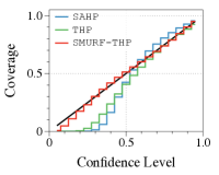
(a) StackOverflow

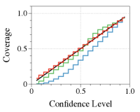
(b) Retweet

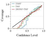
(c) MIMIC-II

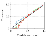
(d) Financial

Figure 1: Coverage of different confidence levels on four datasets.

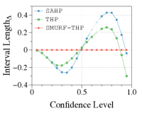
(a) StackOverflow

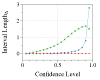
(b) Retweet

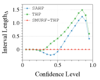
(c) MIMIC-II

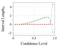
(d) Financial

Figure 2: Interval Length of different confidence levels on four datasets. We minus the interval length of all methods with the length of SMURF-THP (denoted as Interval Length_Δ) to better show the differences.

Distribution of Samples. We visualize the distribution of samples generated by SMURF-THP for several events to study the predicted intensity and present them in Figure 3. A large proportion of the samples stay close to value 0, which is reasonable since most of the events occur within a short time after the previous one. Distributions vary as time goes further. Figure 3(c) and Figure 3(d) exhibit that SMURF-THP can still present tiny peaks around the ground truth value, indicating that our model can still capture the effect of historical events. Yet, the generated samples may be inaccurate due to the huge randomness around the large values of arrival time.

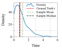
(a) Ground truth $t\in[0,1)$

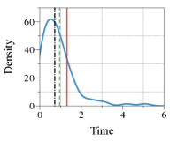
(b) Ground truth $t\in[1,2)$

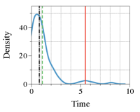
(c) Ground truth $t\in[4,5)$

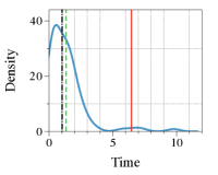
(d) Ground truth $t\in[5,6)$

Figure 3: Distribution of samples generated by SMURF-THP and the ground truth value $t$ in the StackOverflow dataset. The green and black lines signify the mean and median values of the samples. Ground truth of the event arrival time $t$ is chosen randomly from time intervals $[0,1),[1,2),[4,5)$, and $[5,6)$.

4.3 Ablation Study

Parametrization. In addition to parametrizing the intensity function, we can also parametrize the score function directly as was done in conventional score-based methods. That is, we can mask the intensity function and directly parametrize the corresponding score function with the neural network. Table 3 summarizes the results on the StackOverflow and Retweet datasets, where $\texttt{SMURF-THP}^{\texttt{s}}$ indicates SMURF-THP with the score function parametrized. Results imply that parametrizing the intensity function fits the sequence better than parametrizing the score function. This might occur because deriving the score function from the intensity implicitly narrows the searching space, which facilitates the model’s convergence.

Table 3: Calibration Score and CRPS of SMURF-THP with two different parametrizations. The superscript s indicates a direct parametrization on the score function as opposed to no superscript indicating a parameterization on the intensity function.

	StackOverflow		Retweet
Methods	$\mathrm{CS}(\%)$	$\mathrm{CRPS}$	$\mathrm{CS}(\%)$	$\mathrm{CRPS}$
$\texttt{SMURF-THP}^{\texttt{s}}$	6.13	0.54	3.92	1.33
SMURF-THP	0.65	0.44	0.71	0.86

Denoising. SMURF-THP adds Gaussian noise to data points and adopts denoising score matching for better performance and computational efficiency. We test the effects of different noise scales $\sigma$ in Figure 4. Compared with training on clean data, adding perturbations effectively improves the performance with a suitable noise scale. Nevertheless, the selection of noise scale is tricky. Adding too small noise will lead to unstable training, which does not cover the low-density regions enough and degrades the performance. A too large noise, on the other hand, over-corrupts the data and alters the distribution significantly from the original one. We simply select $\sigma$ by grid search in the above experiments and leave auto-selection for future work.

Sampling Method. We inspect variants of our sampling algorithm, including Langevin Dynamics without the denoising step and Mirror Langevin Dynamics, on two datasets. Table 4 summarizes the results. Langevin with the denoising step yields the best performance since the denoising step corrects the perturbed distribution and ensures non-negativity. Mirror Langevin yields the worst results, likely due to the fact that SMURF-THP learns the score of a perturbed distribution which is not restricted to a constrained region.

Table 4: Calibration Score and CRPS of SMURF-THP with different sampling algorithms on StackOverflow and Retweet datasets.

	StackOverflow		Retweet
Sampling Algorithm	$\mathrm{CS}(\%)$	$\mathrm{CRPS}$	$\mathrm{CS}(\%)$	$\mathrm{CRPS}$
Langevin+DS	0.65	0.44	0.71	0.86
Langevin	0.87	0.46	1.38	0.92
Mirror Langevin	8.88	0.69	6.73	1.29

Accuracy with ground truth timestamp. We measure the type prediction accuracy of SMURF-THP given ground truth event time as the inputs of the classifier $g$. As presented in Table 5, the prediction accuracy of SMURF-THP exhibits an obvious increase compared with results in Table 2. This indicates the value of arrival time for type prediction and also demonstrates that SMURF-THP successfully captures the time-type dependencies.

Table 5: Event type prediction accuracy of SMURF-THP given ground truth event time as the inputs.

	SMURF-THP
Dataset	Acc(%)
StackOverflow	48.38
Retweet	61.65
MIMIC-II	83.84
Financial	61.62

Hyperparameter Sensitivity. We examine the sensitivity of the hyperparameter $\alpha$ in the training objectives to our model’s prediction performance on the StackOverflow dataset. As shown in Figure 5, the Calibration Score and CRPS become lower as $\alpha$ grows, while the accuracy worsens. This accords with intuition since a larger $\alpha$ indicates more attention on fitting event time and less on predicting event type. In the above experiments, we choose the biggest $\alpha$ that can achieve comparable accuracy with THP.

We also train SMURF-THP with different volumes of training data to study its generalization ability. We train the model on different ratios of the dataset and present the performance in Figure 6 and Figure 7. As shown, all metrics go better as we feed more training data. Compared to the Retweet dataset, SMURF-THP is more sensitive to training ratio on the StackOverflow dataset. This is due to that the StackOverflow dataset contains less events than the Retweet, thereby SMURF-THP requires larger proportion to learn the distribution.

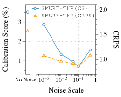
(a) Retweet

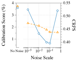
(b) StackOverflow

Figure 4: Comparison of Calibration Score and CRPS of SMURF-THP with different noise scales and with no noise added.

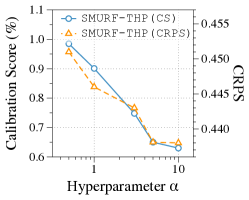
(a) Calibration Score and CRPS

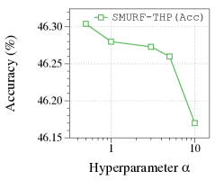
(b) Accuracy

Figure 5: Sensitivity of the hyperparameter $\alpha$ in the training objective to prediction performance.

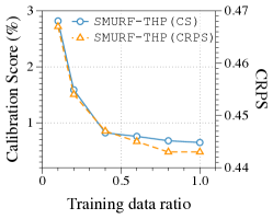
(a) StackOverflow

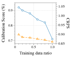
(b) Retweet

Figure 6: Calibration Score and CRPS of SMURF-THP trained with different ratios of the StackOverflow and Retweet datasets.

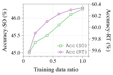
Figure 7: Prediction Accuracy of SMURF-THP trained with different ratio of the StackOverflow and Retweet datasets.

5 Discussion and Conclusion

We acknowledge the existence of several studies that adopt non-likelihood-based estimators to circumvent the intractable integral within the log-likelihood computation. We present our discussions on these works below. Xiao et al., (2017) trains the model to directly predict the next event’s time and type through a summation of Mean Squared Error (MSE) and cross-entropy loss. However, their model does not construct an explicit intensity function and hence doesn’t support flexible sampling and uncertainty quantification. TPPRL (Li et al.,, 2018) employs reinforcement learning (RL) for learning an events generation policy, but they concentrate on the temporal point process (TPP) rather than the marked temporal point process (MTPP), which is the focus of our work. Furthermore, they presume the intensity function to be constant between timestamps, a limitation that hampers the accurate capture of the point process’s temporal dynamics. Upadhyay et al., (2018) applies RL for MTPP which trains a policy to maximize feedback from the environment. Similar to TPPRL, it assumes a very stringent intensity function, e.g., in exponential forms, which is oversimplified to capture the complex point process in real-world applications. INITIATOR (Guo et al.,, 2018) and NCE-TPP (Mei et al.,, 2020) are both based on noise-contrastive estimations for MTPP. However, they utilize the likelihood objective for training the noise generation network, which consequently reintroduces the intractable integral. In our experiments, we include NCE-TPP’s performance, as its authors have demonstrated it outperforms INITIATOR.

Several other works (Wang et al.,, 2020; Fox et al.,, 2016) explore different scopes of uncertainty quantification for the Hawkes process. That is, they provide uncertainty quantification for the parameters in conventional Hawkes process models, whereas we focus on uncertainty quantification for the predicted arrival time.

In this work, we present SMURF-THP, a score-based method for training Transformer Hawkes process models and quantifying prediction uncertainty. Our proposed model adopts score matching as the training objective to avoid intractable computations in conventional Hawkes process models. Moreover, with the learnt score function, we can sample arrival time of events using the Langevin Dynamics. This enables uncertainty quantification by calculating the associated confidence interval. Experiments on various real-world datasets demonstrate that SMURF-THP achieves state-of-the-art performance in terms of Calibration Score, CRPS and Interval Length.

Appendix A Training Detail

Table 6: Summary of hyperparameters used in training.

Dataset	#head	#layer	$d_{\mathrm{model}}$	$d_{k}=d_{v}$	$d_{\mathrm{hidden}}$	dropout	batch	lr	noise scale	Langevin step size $\epsilon$	#step
StackOverflow	4	4	64	16	256	0.1	4	1e-4	1e-1	5e-2	1000
Retweet	3	3	64	16	256	0.1	16	5e-3	5e-2	1e-3	5000
MIMIC-II	3	3	64	16	256	0.1	1	1e-4	1e-1	2e-2	1000
Financial	6	6	128	64	2048	0.1	1	1e-4	5e-2	5e-3	3000

For all datasets used in the experiments, we employ the same data pre-processing and train-dev-test split as Du et al., (2016) and Mei and Eisner, (2017). Please found more details and downloadable links in the aforementioned papers. In addition, we apply normalization to the Retweet, MIMIC-II and MemeTrack datasets to keep the time scale consistent. The hyper-parameters we use are summarized in Table 6. We adopt the Adam optimizer and train all models with 50 epochs using an NVIDIA Tesla P100 GPU. The number of perturbation and samples are set to be 100, increasing which may improve model’s performance.

References

- Bacry et al., (2015) Bacry, E., Mastromatteo, I., and Muzy, J.-F. (2015). Hawkes processes in finance. Market Microstructure and Liquidity, 1(01):1550005.
- Du et al., (2016) Du, N., Dai, H., Trivedi, R., Upadhyay, U., Gomez-Rodriguez, M., and Song, L. (2016). Recurrent marked temporal point processes: Embedding event history to vector. In KDD, pages 1555–1564. ACM.
- Efron, (2011) Efron, B. (2011). Tweedie’s formula and selection bias. Journal of the American Statistical Association, 106(496):1602–1614. PMID: 22505788.
- Fox et al., (2016) Fox, E. W., Schoenberg, F. P., and Gordon, J. S. (2016). Spatially inhomogeneous background rate estimators and uncertainty quantification for nonparametric hawkes point process models of earthquake occurrences.
- Guo et al., (2018) Guo, R., Li, J., and Liu, H. (2018). INITIATOR: noise-contrastive estimation for marked temporal point process. In IJCAI, pages 2191–2197. ijcai.org.
- Hawkes, (1971) Hawkes, A. G. (1971). Spectra of some self-exciting and mutually exciting point processes. Biometrika, 58(1):83–90.
- Hsieh et al., (2018) Hsieh, Y., Kavis, A., Rolland, P., and Cevher, V. (2018). Mirrored langevin dynamics. In NeurIPS, pages 2883–2892.
- Hyvärinen, (2005) Hyvärinen, A. (2005). Estimation of non-normalized statistical models by score matching. J. Mach. Learn. Res., 6:695–709.
- Hyvärinen and Dayan, (2005) Hyvärinen, A. and Dayan, P. (2005). Estimation of non-normalized statistical models by score matching. Journal of Machine Learning Research, 6(4).
- Jordan et al., (2017) Jordan, A., Krüger, F., and Lerch, S. (2017). Evaluating probabilistic forecasts with scoringrules.
- Leskovec and Krevl, (2014) Leskovec, J. and Krevl, A. (2014). SNAP Datasets: Stanford large network dataset collection. http://snap.stanford.edu/data.
- Li et al., (2018) Li, S., Xiao, S., Zhu, S., Du, N., Xie, Y., and Song, L. (2018). Learning temporal point processes via reinforcement learning. In NeurIPS, pages 10804–10814.
- Mei and Eisner, (2017) Mei, H. and Eisner, J. (2017). The neural hawkes process: A neurally self-modulating multivariate point process. In NIPS, pages 6754–6764.
- Mei et al., (2020) Mei, H., Wan, T., and Eisner, J. (2020). Noise-contrastive estimation for multivariate point processes. In NeurIPS.
- Omi et al., (2019) Omi, T., Ueda, N., and Aihara, K. (2019). Fully neural network based model for general temporal point processes. In NeurIPS, pages 2120–2129.
- Sahani et al., (2016) Sahani, M., Bohner, G., and Meyer, A. (2016). Score-matching estimators for continuous-time point-process regression models. In 2016 IEEE 26th International Workshop on Machine Learning for Signal Processing (MLSP), pages 1–5. IEEE.
- Song and Ermon, (2019) Song, Y. and Ermon, S. (2019). Generative modeling by estimating gradients of the data distribution. In NeurIPS, pages 11895–11907.
- Song et al., (2019) Song, Y., Garg, S., Shi, J., and Ermon, S. (2019). Sliced score matching: A scalable approach to density and score estimation. In UAI, volume 115 of Proceedings of Machine Learning Research, pages 574–584. AUAI Press.
- Upadhyay et al., (2018) Upadhyay, U., De, A., and Rodriguez, M. G. (2018). Deep reinforcement learning of marked temporal point processes. In NeurIPS, pages 3172–3182.
- Vaswani et al., (2017) Vaswani, A., Shazeer, N., Parmar, N., Uszkoreit, J., Jones, L., Gomez, A. N., Kaiser, L., and Polosukhin, I. (2017). Attention is all you need. In NIPS, pages 5998–6008.
- Vincent, (2011) Vincent, P. (2011). A connection between score matching and denoising autoencoders. Neural Comput., 23(7):1661–1674.
- Wang et al., (2020) Wang, H., Xie, L., Cuozzo, A., Mak, S., and Xie, Y. (2020). Uncertainty quantification for inferring hawkes networks. In NeurIPS.
- Wang et al., (2018) Wang, L., Zhang, W., He, X., and Zha, H. (2018). Supervised reinforcement learning with recurrent neural network for dynamic treatment recommendation. In Proceedings of the 24th ACM SIGKDD international conference on knowledge discovery & data mining, pages 2447–2456.
- Welling and Teh, (2011) Welling, M. and Teh, Y. W. (2011). Bayesian learning via stochastic gradient langevin dynamics. In ICML, pages 681–688. Omnipress.
- Xiao et al., (2017) Xiao, S., Yan, J., Yang, X., Zha, H., and Chu, S. M. (2017). Modeling the intensity function of point process via recurrent neural networks. In AAAI, pages 1597–1603. AAAI Press.
- Yang et al., (2011) Yang, S.-H., Long, B., Smola, A., Sadagopan, N., Zheng, Z., and Zha, H. (2011). Like like alike: joint friendship and interest propagation in social networks. In Proceedings of the 20th international conference on World wide web, pages 537–546.
- Yu et al., (2019) Yu, S., Drton, M., and Shojaie, A. (2019). Generalized score matching for non-negative data. J. Mach. Learn. Res., 20:76:1–76:70.
- Yu et al., (2022) Yu, S., Drton, M., and Shojaie, A. (2022). Generalized score matching for general domains. Information and Inference: A Journal of the IMA, 11(2):739–780.
- Zhang et al., (2020) Zhang, Q., Lipani, A., Kirnap, Ö., and Yilmaz, E. (2020). Self-attentive hawkes process. In ICML, volume 119 of Proceedings of Machine Learning Research, pages 11183–11193. PMLR.
- Zhao et al., (2015) Zhao, Q., Erdogdu, M. A., He, H. Y., Rajaraman, A., and Leskovec, J. (2015). SEISMIC: A self-exciting point process model for predicting tweet popularity. In KDD, pages 1513–1522. ACM.
- Zhu et al., (2021) Zhu, S., Zhang, M., Ding, R., and Xie, Y. (2021). Deep fourier kernel for self-attentive point processes. In AISTATS, volume 130 of Proceedings of Machine Learning Research, pages 856–864. PMLR.
- Zuo et al., (2020) Zuo, S., Jiang, H., Li, Z., Zhao, T., and Zha, H. (2020). Transformer hawkes process. In ICML, volume 119 of Proceedings of Machine Learning Research, pages 11692–11702. PMLR.