Covariance Blocking and Whitening Method for Successive Relative Transfer Function Vector Estimation in Multi-Speaker Scenarios

Abstract

This paper addresses the challenge of estimating the relative transfer function (RTF) vectors of multiple speakers in a noisy and reverberant environment. More specifically, we consider a scenario where two speakers activate successively. In this scenario, the RTF vector of the first speaker can be estimated in a straightforward way and the main challenge lies in estimating the RTF vector of the second speaker during segments where both speakers are simultaneously active. To estimate the RTF vector of the second speaker the so-called blind oblique projection (BOP) method determines the oblique projection operator that optimally blocks the second speaker. Instead of blocking the second speaker, in this paper we propose a covariance blocking and whitening (CBW) method, which first blocks the first speaker and applies whitening using the estimated noise covariance matrix and then estimates the RTF vector of the second speaker based on a singular value decomposition. When using the estimated RTF vectors of both speakers in a linearly constrained minimum variance beamformer, simulation results using real-world recordings for multiple speaker positions demonstrate that the proposed CBW method outperforms the conventional BOP and covariance whitening methods in terms of signal-to-interferer-and-noise ratio improvement.

Index Terms—  successive speakers, RTF vector estimation, LCMV beamforming

1 Introduction

In many hands-free speech communication systems such as hearing aids, mobile phones and smart speakers, interfering sounds and ambient noise may degrade the speech quality and intelligibility of the recorded microphone signals [1]. When multiple microphones are available, beamforming is a widely used technique to enhance a target speaker and suppress interfering speakers and noise [2, 3, 4]. One commonly used beamforming technique is the linearly constrained minimum variance (LCMV) beamformer [2, 5, 6, 7], which requires estimates of the relative transfer function (RTF) vectors of the target speaker and interfering speakers, as well as an estimate of the noise covariance matrix.

Over the last decades, several methods have been proposed to estimate the RTF vector of a single speaker in a noisy environment, e.g., based on (weighted) least-squares [8, 9], using covariance subtraction and covariance whitening [10, 11, 12, 13, 14], using manifold learning [15] or by jointly estimating the RTF vector and power spectral densities [16, 17]. The state-of-the-art covariance whitening (CW) method estimates the RTF vector of a single speaker by de-whitening the principal eigenvector of the whitened noisy covariance matrix, where an estimate of the noise covariance matrix is used for the whitening.

In contrast to estimating the RTF vector of a single speaker, estimating the RTF vectors of multiple speakers that are simultaneously active is more challenging. In a multi-speaker scenario, the CW method can only estimate a subspace spanning the RTF vectors of all speakers, instead of the individual RTF vectors [11]. Methods to estimate the RTF vectors of multiple speakers have been proposed, e.g., using an expectation maximization algorithm [18], utilizing subframes to perform factor analysis [19] or using joint diagonalization [20]. A drawback of the methods is the permutation ambiguity, requiring a method to correctly assign the estimated RTF vectors to the speakers in each frequency band. An RTF vector update method using Procrustes analysis was proposed in [21].

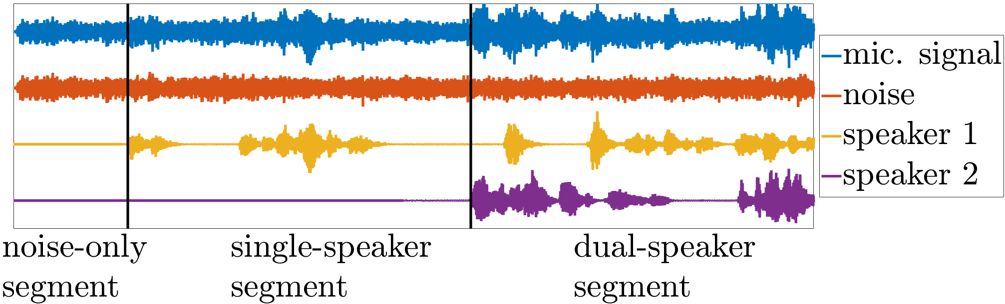
Figure 1: Example of successive speaker scenario with two speakers, depicting a microphone signal and its speech and noise components for three different segments.

In this paper, we consider a specific scenario with two speakers that activate successively (see Figure 1). In this scenario, the RTF vector of the first speaker can be estimated in the single-speaker segment, e.g., using the CW method with an estimate of the noise covariance matrix from the noise-only segment. The focus of this paper is on estimating the RTF vector of the second speaker in the dual-speaker segment, using available estimates of the noise covariance matrix and the RTF vector of the first speaker. First, we consider a modified version of the conventional CW method, where the whitening is performed using the undesired covariance matrix (estimated in the single-speaker segment) instead of the noise covariance matrix. A disadvantage of this method is its dependence on the possibly time-varying power spectral density (PSD) of the first speaker. Second, we consider the blind oblique projection (BOP) method [22], which estimates the RTF vector of the second speaker by determining the oblique projection operator which optimally blocks the unknown second speaker. A disadvantage of the BOP method is that it assumes a sufficiently large signal-to-noise ratio (SNR). Third, we propose the covariance blocking and whitening (CBW) method, which overcomes the mentioned disadvantages of the CW and BOP methods, i.e. it is independent of the PSD of the first speaker and does not assume a large SNR. Instead of blocking the unknown second speaker as done by the BOP method, the CBW method uses a residual maker matrix to block the known RTF vector of the first speaker, followed by noise whitening. Since the blocking of the first speaker leads to a dimension reduction, it is shown that a singular value decomposition (SVD) instead of an eigenvalue decomposition is required to extract the RTF vector of the second speaker. When using the estimated RTF vectors in an LCMV beamformer, simulation results using real-world recordings for multiple speaker positions and signal-to-interferer ratios (SIRs) demonstrate that the proposed CBW method outperforms the conventional methods in terms of signal-to-interferer-and-noise ratio (SINR) improvement.

2 Signal Model

We consider a scenario where two speakers are successively activated and captured by an array with $M$ microphones in a noisy and reverberant environment. Figure 1 depicts this specific scenario, which can be divided into three time segments: a noise-only segment $(s=1)$, a single-speaker segment containing the first speaker and noise $(s=2)$, and a dual-speaker segment containing both speakers and noise $(s=3)$, where $s$ denotes the segment index. We assume that the segment boundaries are known. Without loss of generality, the first speaker is considered the interfering speaker, whereas the second speaker is considered the target speaker. We assume that for the whole signal duration the scenario is spatially stationary, i.e., the speakers do not move. The short-time Fourier transform (STFT) coefficients of the microphone signals at time frame $t$ are denoted by

$$\mathbf{y}_{t}=\begin{bmatrix}y_{1,t}&\cdots&y_{M,t}\end{bmatrix}^{\mathrm{T}}\in\mathbb{C}^{M\times 1},$$ (1)

where $\{\cdot\}^{\mathrm{T}}$ denotes the transpose operator. The frequency index is omitted as it is assumed that each frequency band is independent and can be processed individually. The multi-channel microphone signal $\mathbf{y}_{t}$ can be written as the sum of the target speaker component $\mathbf{x}_{t}$ and the undesired component $\mathbf{v}_{t}$, which consists of the interfering speaker component $\mathbf{u}_{t}$ and the noise component $\mathbf{n}_{t}$, i.e.,

$$\mathbf{y}_{t}=\mathbf{x}_{t}+\underbrace{\mathbf{u}_{t}+\mathbf{n}_{t}}_{\mathbf{v}_{t}}=\mathbf{h}x_{r,t}+\mathbf{g}u_{r,t}+\mathbf{n}_{t},$$ (2)

where the vectors $\mathbf{x}_{t}$, $\mathbf{u}_{t}$, $\mathbf{n}_{t}$ and $\mathbf{v}_{t}$ are defined similarly as in (1). Assuming sufficiently large STFT frames, the speaker components $\mathbf{x}_{t}$ and $\mathbf{u}_{t}$ are modeled as the multiplication of the STFT coefficient of a reference microphone (denoted by $r$) with the respective time-invariant RTF vectors $\mathbf{h}$ and $\mathbf{g}$ [23]. Note that the reference entry of both RTF vectors equals $1$. Assuming all signal components in (2) to be uncorrelated, the noisy covariance matrix for each time segment $s$ is given by

$$\mathbf{R}_{\mathbf{y},s}=\underbrace{\mathbf{h}\phi_{x,s}\mathbf{h}^{\mathrm{H}}}_{\mathbf{R}_{\mathbf{x},s}}+\underbrace{\underbrace{\mathbf{g}\phi_{u,s}\mathbf{g}^{\mathrm{H}}}_{\mathbf{R}_{\mathbf{u},s}}+\mathbf{R}_{\mathbf{n}}}_{\mathbf{R}_{\mathbf{v},s}},$$ (3)

where $\{\cdot\}^{\mathrm{H}}$ denotes the conjugate transpose operator. The matrices $\mathbf{R}_{\mathbf{u},s}$ and $\mathbf{R}_{\mathbf{x},s}$ denote the rank-1 covariance matrices of the first and second speaker, respectively, $\mathbf{R}_{\mathbf{n}}$ and $\mathbf{R}_{\mathbf{v},s}$ denote the full-rank covariance matrices of the noise and undesired component, respectively, and $\phi_{x,s}=\mathcal{E}\{\left\lvert x_{r}\right\rvert^{2}\}$ and $\phi_{u,s}=\mathcal{E}\{\left\lvert u_{r}\right\rvert^{2}\}$ denote the PSDs with $\mathcal{E}\{\cdot\}$ the expectation operator. Note that $\phi_{x,1}=\phi_{u,1}=\phi_{x,2}=0$ for the considered successive speaker scenario.

3 LCMV beamformer

To extract the second speaker (target speaker) and suppress the first speaker (interfering speaker) and noise in the dual-speaker segment $(s=3)$, we will use an LCMV beamformer. The LCMV beamformer minimizes the noise PSD subject to linear constraints, which aim at keeping the target speaker distortionless and reducing the interfering speaker [2, 5, 6], i.e.,

$$\mathbf{w}=\operatorname*{argmin}_{\tilde{\mathbf{w}}}\left(\tilde{\mathbf{w}}^{\mathrm{H}}\mathbf{R}_{\mathbf{n}}\tilde{\mathbf{w}}\right)\quad\mathrm{s.t.}\quad\begin{matrix}\tilde{\mathbf{w}}^{\mathrm{H}}\mathbf{x}_{t}=x_{r,t}\\ \tilde{\mathbf{w}}^{\mathrm{H}}\mathbf{u}_{t}=\delta u_{r,t}\end{matrix},$$ (4)

where $\delta$ denotes the scaling factor to reduce the interfering speaker. The widely known solution to the minimization problem in (4) is given by

$$\boxed{\mathbf{w}=\mathbf{R}_{\mathbf{n}}^{-1}\mathbf{C}\left(\mathbf{C}^{\mathrm{H}}\mathbf{R}_{\mathbf{n}}^{-1}\mathbf{C}\right)^{-1}\begin{bmatrix}1\\ \delta\end{bmatrix}}$$ (5)

where the constraint matrix $\mathbf{C}$ contains the RTF vectors of both speakers, i.e., $\mathbf{C}=\begin{bmatrix}\mathbf{h}&\mathbf{g}\end{bmatrix}$. Applying the LCMV beamformer to the microphone signals yields the enhanced signal

$$\mathbf{z}_{t}=\mathbf{w}^{\mathrm{H}}\mathbf{y}_{t}.$$ (6)

As can be seen in (5), the LCMV beamformer requires an estimate of the noise covariance matrix $\mathbf{R}_{\mathbf{n}}$, which can be easily obtained in the noise-only segment, and estimates of the RTF vectors of both speakers. Section 3.1 discusses a method to estimate the RTF vector $\mathbf{g}$ of the first speaker. The main focus of the paper is on estimating the RTF vector $\mathbf{h}$ of the second speaker, for which several methods will be presented in Section 4 and Section 5.

3.1 Covariance Whitening (CW)

In the single-speaker segment $(s=2)$ where $\phi_{x,2}=0$, the RTF vector $\mathbf{g}$ of the first speaker can be estimated using the state-of-the-art CW method [11, 12, 14]. First, the noisy covariance matrix $\mathbf{R}_{\mathbf{y},2}$ in (3) is whitened using a square-root decomposition of the noise covariance matrix $\mathbf{R}_{\mathbf{n}}=\mathbf{R}_{\mathbf{n}}^{\nicefrac{{\mathrm{H}}}{{2}}}\mathbf{R}_{\mathbf{n}}^{\nicefrac{{1}}{{2}}}$, i.e.,

$$\mathbf{R}_{\mathbf{n}}^{-\nicefrac{{\mathrm{H}}}{{2}}}\mathbf{R}_{\mathbf{y},2}\mathbf{R}_{\mathbf{n}}^{-\nicefrac{{1}}{{2}}}=\mathbf{R}_{\mathbf{n}}^{-\nicefrac{{\mathrm{H}}}{{2}}}\mathbf{g}\phi_{u,2}\mathbf{g}^{\mathrm{H}}\mathbf{R}_{\mathbf{n}}^{-\nicefrac{{1}}{{2}}}+\mathbf{I}_{M}.$$ (7)

This whitening operation spatially decorrelates the noise, transforming the noise covariance matrix into an identity matrix. From (7), the RTF vector $\mathbf{g}$ can then be estimated as the normalized de-whitened principal eigenvector of the whitened noisy covariance matrix, i.e.,

$$\boxed{\widehat{\mathbf{g}}=\nicefrac{{\tilde{\mathbf{g}}}}{{\mathbf{e}_{r}^{\mathrm{T}}\tilde{\mathbf{g}}}}\quad\mathrm{with}\quad\tilde{\mathbf{g}}=\mathbf{R}_{\mathbf{n}}^{\nicefrac{{\mathrm{H}}}{{2}}}\mathcal{P}\{\mathbf{R}_{\mathbf{n}}^{-\nicefrac{{\mathrm{H}}}{{2}}}\mathbf{R}_{\mathbf{y},2}\mathbf{R}_{\mathbf{n}}^{-\nicefrac{{1}}{{2}}}\}}$$ (8)

where $\mathbf{e}_{r}=\begin{bmatrix}0&\cdots&1&\cdots&0\end{bmatrix}^{\mathrm{T}}$ is an $M$-dimensional selection vector of the reference microphone $r$ and $\mathcal{P}\{\cdot\}$ denotes the principal eigenvector operator.

4 Conventional RTF Estimation Methods

In this section, we describe two conventional methods to estimate the RTF vector $\mathbf{h}$ of the second speaker in the dual-speaker segment, where both speakers and noise are present, assuming estimates of the noise covariance matrix $\mathbf{R}_{\mathbf{n}}$, the undesired covariance matrix $\mathbf{R}_{\mathbf{v}}$ and the RTF vector $\mathbf{g}$ of the first speaker to be available.

4.1 CW with undesired covariance matrix (CWu)

In Section 3.1 the CW method was discussed to estimate the RTF vector of the first speaker. Although the CW method typically performs whitening using the estimated noise covariance matrix $\mathbf{R}_{\mathbf{n}}$, this method can also be used to estimate the RTF vector of the second speaker in the dual-speaker segment by performing whitening with the undesired covariance matrix $\mathbf{R}_{\mathbf{v}}$ (estimated during the single-speaker segment), i.e.,

$$\boxed{\widehat{\mathbf{h}}^{(\mathrm{CW})}=\nicefrac{{\tilde{\mathbf{h}}}}{{\mathbf{e}_{r}^{\mathrm{T}}\tilde{\mathbf{h}}}}\quad\mathrm{with}\quad\tilde{\mathbf{h}}=\mathbf{R}_{\mathbf{v},2}^{\nicefrac{{\mathrm{H}}}{{2}}}\mathcal{P}\{\mathbf{R}_{\mathbf{v},2}^{-\nicefrac{{\mathrm{H}}}{{2}}}\mathbf{R}_{\mathbf{y},3}\mathbf{R}_{\mathbf{v},2}^{-\nicefrac{{1}}{{2}}}\}}$$ (9)

This will be referred to as CW with the undesired covariance matrix (CWu). It should be noted that since the PSD of the first speaker in the single-speaker segment $\phi_{u,2}$ may not be the same as in the dual-speaker segment $\phi_{u,3}$, the undesired covariance matrix $\mathbf{R}_{\mathbf{v},2}$ used for whitening may strongly deviate form the undesired covariance matrix $\mathbf{R}_{\mathbf{v},3}$, resulting in a biased RTF vector estimate.

4.2 Blind Oblique Projection (BOP)

Avoiding the influence of the time-varying PSD $\phi_{u}$ of the first speaker, the BOP method proposed in [22] estimates the RTF vector $\mathbf{h}$ of the second speaker by blocking the second speaker as much as possible while keeping the first speaker distortionless. This can be achieved by the so-called oblique projection operator [24] with vector variable $\bm{\theta}$, defined as

$$\mathbf{P}^{\angle}_{\mathbf{g}\bm{\theta}}=\mathbf{g}\left(\mathbf{g}^{\mathrm{H}}\mathbf{P}^{\perp}_{\bm{\theta}}\mathbf{g}\right)^{-1}\mathbf{g}^{\mathrm{H}}\mathbf{P}^{\perp}_{\bm{\theta}},$$ (10)

where $\mathbf{P}^{\perp}_{\bm{\theta}}$ denotes the residual maker matrix

$$\mathbf{P}^{\perp}_{\bm{\theta}}=\mathbf{I}_{M}-\nicefrac{{\bm{\theta}\bm{\theta}^{\mathrm{H}}}}{{\bm{\theta}^{\mathrm{H}}\bm{\theta}}}.$$ (11)

The oblique projection operator in (10) keeps the RTF vector of the first speaker, i.e., $\mathbf{P}^{\angle}_{\mathbf{g}\bm{\theta}}\mathbf{g}=\mathbf{g}$, but blocks the range of the vector $\bm{\theta}$, i.e., $\mathbf{P}^{\angle}_{\mathbf{g}\bm{\theta}}\bm{\theta}=\mathbf{0}_{M\times 1}$. Applying the oblique projection operator in (10) to (3) in the dual-speaker segment and taking the trace yields

$$\mathrm{Tr}\{\mathbf{P}^{\angle}_{\mathbf{g}\bm{\theta}}\mathbf{R}_{\mathbf{y},3}\mathbf{P}^{\angle\mathrm{H}}_{\mathbf{g}\bm{\theta}}\}=\phi_{x,3}\mathbf{h}^{\mathrm{H}}\mathbf{P}^{\angle\mathrm{H}}_{\mathbf{g}\bm{\theta}}\mathbf{P}^{\angle}_{\mathbf{g}\bm{\theta}}\mathbf{h}+\phi_{u,3}\mathbf{g}^{\mathrm{H}}\mathbf{g}\\ +\mathrm{Tr}\{\mathbf{P}^{\angle}_{\mathbf{g}\bm{\theta}}\mathbf{R}_{\mathbf{n}}\mathbf{P}^{\angle\mathrm{H}}_{\mathbf{g}\bm{\theta}}\}.$$ (12)

In [22] a sufficiently large SNR was assumed, such that the noise term $\mathrm{Tr}\{\mathbf{P}^{\angle}_{\mathbf{g}\bm{\theta}}\mathbf{R}_{\mathbf{n}}\mathbf{P}^{\angle\mathrm{H}}_{\mathbf{g}\bm{\theta}}\}$ in (12) can be neglected. Since the term $\phi_{u,3}\mathbf{g}^{\mathrm{H}}\mathbf{g}$ is a constant, it can be seen that the power of the projected noisy covariance matrix $\mathrm{Tr}\{\mathbf{P}^{\angle}_{\mathbf{g}\bm{\theta}}\mathbf{R}_{\mathbf{y},3}\mathbf{P}^{\angle\mathrm{H}}_{\mathbf{g}\bm{\theta}}\}$ is minimized when the oblique projection operator $\mathbf{P}^{\angle}_{\mathbf{g}\bm{\theta}}$ blocks the RTF vector $\mathbf{h}$ of the second speaker in (12), which is achieved if the vector $\bm{\theta}$ points in the same direction as $\mathbf{h}$. Therefore an estimate of the RTF vector of the second speaker can be obtained as

$$\boxed{\widehat{\mathbf{h}}^{(\mathrm{BOP})}=\nicefrac{{\tilde{\mathbf{h}}}}{{\mathbf{e}_{r}^{\mathrm{T}}\tilde{\mathbf{h}}}}\quad\mathrm{with}\quad\tilde{\mathbf{h}}=\operatorname*{argmin}_{\bm{\theta}}\left(\mathrm{Tr}\{\mathbf{P}^{\angle}_{\mathbf{g}\bm{\theta}}\mathbf{R}_{\mathbf{y},3}\mathbf{P}^{\angle\mathrm{H}}_{\mathbf{g}\bm{\theta}}\}\right)}$$ (13)

Since no closed-form solution for the optimization problem in (13) exists, it was proposed in [22] to use a gradient-descent method. For faster computational speed and higher robustness, in this paper we provided the analytical gradient of (13) to the sequential-quadratic-programming method [25], implemented within the Matlab optimization toolbox [26].

5 Covariance Blocking and Whitening

Instead of whitening using the undesired covariance matrix $\mathbf{R}_{\mathbf{v}}$ as in the CWu method, in this section we propose a method that blocks the known first speaker before noise whitening. This can be seen as introducing blocking of the first speaker to the conventional CW method, to enable estimation of the individual RTF vector of the second speaker. It should be noted that this blocking approach differs fundamentally from the BOP method, where the unknown second speaker is blocked instead of the known first speaker. In principle, the RTF vector $\mathbf{g}$ of the first speaker can be blocked by applying the residual maker matrix

$$\mathbf{P}^{\perp}_{{\mathbf{g}}}=\mathbf{I}_{M}-\nicefrac{{\mathbf{g}\mathbf{g}^{\mathrm{H}}}}{{\left(\mathbf{g}^{\mathrm{H}}\mathbf{g}\right)}}$$ (14)

with $\mathbf{g}^{\mathrm{H}}\mathbf{P}^{\perp}_{{\mathbf{g}}}=\mathbf{0}_{1\times M}$, to (3) from the right in the dual-speaker segment, yielding

$$\mathbf{R}_{\mathbf{y},3}\mathbf{P}^{\perp}_{\mathbf{g}}={\mathbf{h}}\phi_{x,3}{\mathbf{h}}^{\mathrm{H}}\mathbf{P}^{\perp}_{{\mathbf{g}}}+\mathbf{R}_{\mathbf{n}}\mathbf{P}^{\perp}_{{\mathbf{g}}}.$$ (15)

It should be noted that since the matrix $\mathbf{P}^{\perp}_{{\mathbf{g}}}$ in (15) has rank $(M-1)$, the noise term $\mathbf{R}_{\mathbf{n}}\mathbf{P}^{\perp}_{{\mathbf{g}}}$ in (15) also has rank $(M-1)$. Since full column rank of the noise term is required to whiten the noise component, we propose to use a dimension-reduced version $\mathbf{P}^{\perp}_{{\mathbf{g},\mathrm{r}}}=\mathbf{P}^{\perp}_{{\mathbf{g}}}\begin{bmatrix}\mathbf{I}_{M-1}&\mathbf{0}_{\left(M-1\right)\times 1}\end{bmatrix}^{\mathrm{T}}\in\mathbb{C}^{M\times M-1}$ of the residual maker matrix $\mathbf{P}^{\perp}_{{\mathbf{g}}}$ instead, i.e.,

$$\mathbf{R}_{\mathbf{y},3}\mathbf{P}^{\perp}_{\mathbf{g},\mathrm{r}}={\mathbf{h}}\phi_{x,3}{\mathbf{h}}^{\mathrm{H}}\mathbf{P}^{\perp}_{{\mathbf{g},\mathrm{r}}}+\mathbf{R}_{\mathbf{n}}\mathbf{P}^{\perp}_{{\mathbf{g},\mathrm{r}}}\in\mathbb{C}^{M\times M-1}.$$ (16)

Whitening the blocked noise term $\mathbf{R}_{\mathbf{n}}\mathbf{P}^{\perp}_{{\mathbf{g},\mathrm{r}}}$ in (16) using its pseudo-inverse denoted by $\{\cdot\}^{+}$, i.e., transforming it to an identity matrix similarly as for the conventional CW method in (7), and subtracting the resulting identity matrix yields

$$\mathbf{R}_{\mathbf{y}}^{\mathrm{w}}=\left(\mathbf{R}_{\mathbf{n}}\mathbf{P}^{\perp}_{{\mathbf{g},\mathrm{r}}}\right)^{+}\mathbf{R}_{\mathbf{y},3}\mathbf{P}^{\perp}_{{\mathbf{g},\mathrm{r}}}-\mathbf{I}_{M-1}=\left(\mathbf{R}_{\mathbf{n}}\mathbf{P}^{\perp}_{{\mathbf{g},\mathrm{r}}}\right)^{+}{\mathbf{h}}\phi_{x}{\mathbf{h}}^{\mathrm{H}}\mathbf{P}^{\perp}_{{\mathbf{g},\mathrm{r}}}.$$ (17)

This set of equations has dimensions $(M-1)\times(M-1)$ in contrast to the signal model in (3) having dimensions $M\times M$. It should be noted that the right side of (17) is given by the outer product of two transformed versions of the RTF vector $\mathbf{h}$ of the second speaker, whereby both transformations only depend on $\mathbf{R}_{\mathbf{n}}$ and $\mathbf{g}$. The transformed versions of the RTF vector can be extracted by means of an SVD, i.e.,

$$\mathbf{q}_{\mathrm{L}}= \;\mathcal{S}_{\mathrm{L}}\{\mathbf{R}_{\mathbf{y}}^{\mathrm{w}}\}=\left(\mathbf{R}_{\mathbf{n}}\mathbf{P}^{\perp}_{{\mathbf{g},\mathrm{r}}}\right)^{+}{\mathbf{h}}\alpha_{\mathrm{L}},$$ (18)

$$\mathbf{q}_{\mathrm{R}}= \;\mathcal{S}_{\mathrm{R}}\{\mathbf{R}_{\mathbf{y}}^{\mathrm{w}}\}=\left(\mathbf{P}^{\perp}_{{\mathbf{g},\mathrm{r}}}\right)^{\mathrm{H}}{\mathbf{h}}\alpha_{\mathrm{R}},$$ (19)

where $\mathcal{S}_{\mathrm{L}}\{\cdot\}$ and $\mathcal{S}_{\mathrm{R}}\{\cdot\}$ denote the principal left and right singular vector operator, respectively, and $\alpha_{\mathrm{L}}$ and $\alpha_{\mathrm{R}}$ are scaling factors. It should be noted that since $\mathbf{q}_{\mathrm{L}}$ and $\mathbf{q}_{\mathrm{R}}$ are $(M-1)$-dimensional vectors, neither vector provides a solution for the $M$-dimensional RTF vector $\mathbf{h}$.

By introducing the scaled RTF vector $\tilde{\mathbf{h}}=\alpha_{\mathrm{L}}\mathbf{h}$ and the weighting factor $\alpha=\nicefrac{{\alpha_{\mathrm{L}}}}{{\alpha_{\mathrm{R}}}}$ and by stacking (18) and (19) into one unified set of equations, we obtain

$$\begin{bmatrix}\mathbf{q}_{\mathrm{L}}\\ \mathbf{q}_{\mathrm{R}}\alpha\end{bmatrix}\overset{!}{=}\mathbf{B}\tilde{\mathbf{h}}\quad\mathrm{with}\quad\mathbf{B}=\begin{bmatrix}\left(\mathbf{R}_{\mathbf{n}}\mathbf{P}_{\mathbf{g},\mathrm{r}}^{\perp}\right)^{+}\\ \left(\mathbf{P}_{\mathbf{g},\mathrm{r}}^{\perp}\right)^{\mathrm{H}}\end{bmatrix}.$$ (20)

This non-linear set of equations contains $2(M-1)$ equations and $M+1$ unknowns ($\tilde{\mathbf{h}}$ and $\alpha$), hence requiring $2(M-1)\geq M+1$, i.e., $M\geq 3$. Inverting $\mathbf{B}$ using its pseudo-inverse and applying it to (20) from the left yields

$$\tilde{\mathbf{h}}\overset{}{=}\mathbf{B}^{+}\begin{bmatrix}\mathbf{q}_{\mathrm{L}}\\ \mathbf{q}_{\mathrm{R}}\alpha\end{bmatrix},$$ (21)

which depends on the unknown $\alpha$. Substituting (21) into (20) leads to

$$\begin{bmatrix}\mathbf{q}_{\mathrm{L}}\\ \mathbf{q}_{\mathrm{R}}\alpha\end{bmatrix}\overset{!}{=}\mathbf{B}\mathbf{B}^{+}\begin{bmatrix}\mathbf{q}_{\mathrm{L}}\\ \mathbf{q}_{\mathrm{R}}\alpha\end{bmatrix}\quad\Rightarrow\quad\mathbf{P}^{\perp}_{\mathbf{B}}\begin{bmatrix}\mathbf{q}_{\mathrm{L}}\\ \mathbf{q}_{\mathrm{R}}\alpha\end{bmatrix}\overset{!}{=}\mathbf{0}_{2(M-1)\times 1},$$ (22)

where $\mathbf{P}^{\perp}_{\mathbf{B}}$ is the residual maker matrix of $\mathbf{B}$ defined similarly to (14). Reformulating (22) using the block decomposition $\mathbf{P}^{\perp}_{\mathbf{B}}=\begin{bmatrix}\mathbf{P}^{\perp,\mathrm{L}}_{\mathbf{B}}&\mathbf{P}^{\perp,\mathrm{R}}_{\mathbf{B}}\end{bmatrix}$ provides a solution for $\alpha$, i.e.,

$$-\mathbf{P}^{\perp,\mathrm{L}}_{\mathbf{B}}\mathbf{q}_{\mathrm{L}}=\mathbf{P}^{\perp,\mathrm{R}}_{\mathbf{B}}\mathbf{q}_{\mathrm{R}}\alpha\quad\Rightarrow\quad\alpha=-\left(\mathbf{P}^{\perp,\mathrm{R}}_{\mathbf{B}}\mathbf{q}_{\mathrm{R}}\right)^{+}\mathbf{P}^{\perp,\mathrm{L}}_{\mathbf{B}}\mathbf{q}_{\mathrm{L}}.$$ (23)

Substituting $\alpha$ in (23) into $\tilde{\mathbf{h}}$ in (21) and applying normalization provides an estimate of the RTF vector of the second speaker, i.e.,

$$\boxed{\widehat{\mathbf{h}}^{(\mathrm{CBW})}=\nicefrac{{\tilde{\mathbf{h}}}}{{\mathbf{e}_{r}^{\mathrm{T}}\tilde{\mathbf{h}}}}\quad\mathrm{with}\quad\tilde{\mathbf{h}}\overset{}{=}\mathbf{B}^{+}\begin{bmatrix}\mathbf{q}_{\mathrm{L}}\\ -\mathbf{q}_{\mathrm{R}}\left(\mathbf{P}^{\perp,\mathrm{R}}_{\mathbf{B}}\mathbf{q}_{\mathrm{R}}\right)^{+}\mathbf{P}^{\perp,\mathrm{L}}_{\mathbf{B}}\mathbf{q}_{\mathrm{L}}\end{bmatrix}}$$ (24)

6 Experimental Results

In this section, we compare the performance of the conventional RTF vector estimation methods (see Section 4) with the proposed CBW method, when using the estimated RTF vectors of the target and interfering speakers (second and first speaker, respectively) in an LCMV beamformer.

6.1 Acoustic Scenario

Figure 2 depicts the acoustic setup. We considered a linear array with 4 microphones with a microphone spacing of $2\text{\,}\mathrm{cm}$, located approximately in the center of an acoustic laboratory $($7\text{\,}\mathrm{m}$\times$6\text{\,}\mathrm{m}$\times$2.7\text{\,}\mathrm{m}$)$ with a reverberation time $T_{60}\approx$500\text{\,}\mathrm{ms}$$. The acoustic scenario consists of constantly active background noise, one interfering speaker active in the interval $\left[$1\text{\,}\mathrm{s}$,$7\text{\,}\mathrm{s}$\right]$ and one target speaker active in the interval $\left[$4\text{\,}\mathrm{s}$,$7\text{\,}\mathrm{s}$\right]$. The target and interfering speech components at the microphones were generated by convolving clean speech signals with room impulse responses measured from loudspeakers at 9 different positions (see Figure 2). Quasi-diffuse noise was generated by playing back uncorrelated babble noise using 4 loudspeakers facing the corners of the laboratory. The sampling frequency was equal to $16\text{\,}\mathrm{kHz}$.

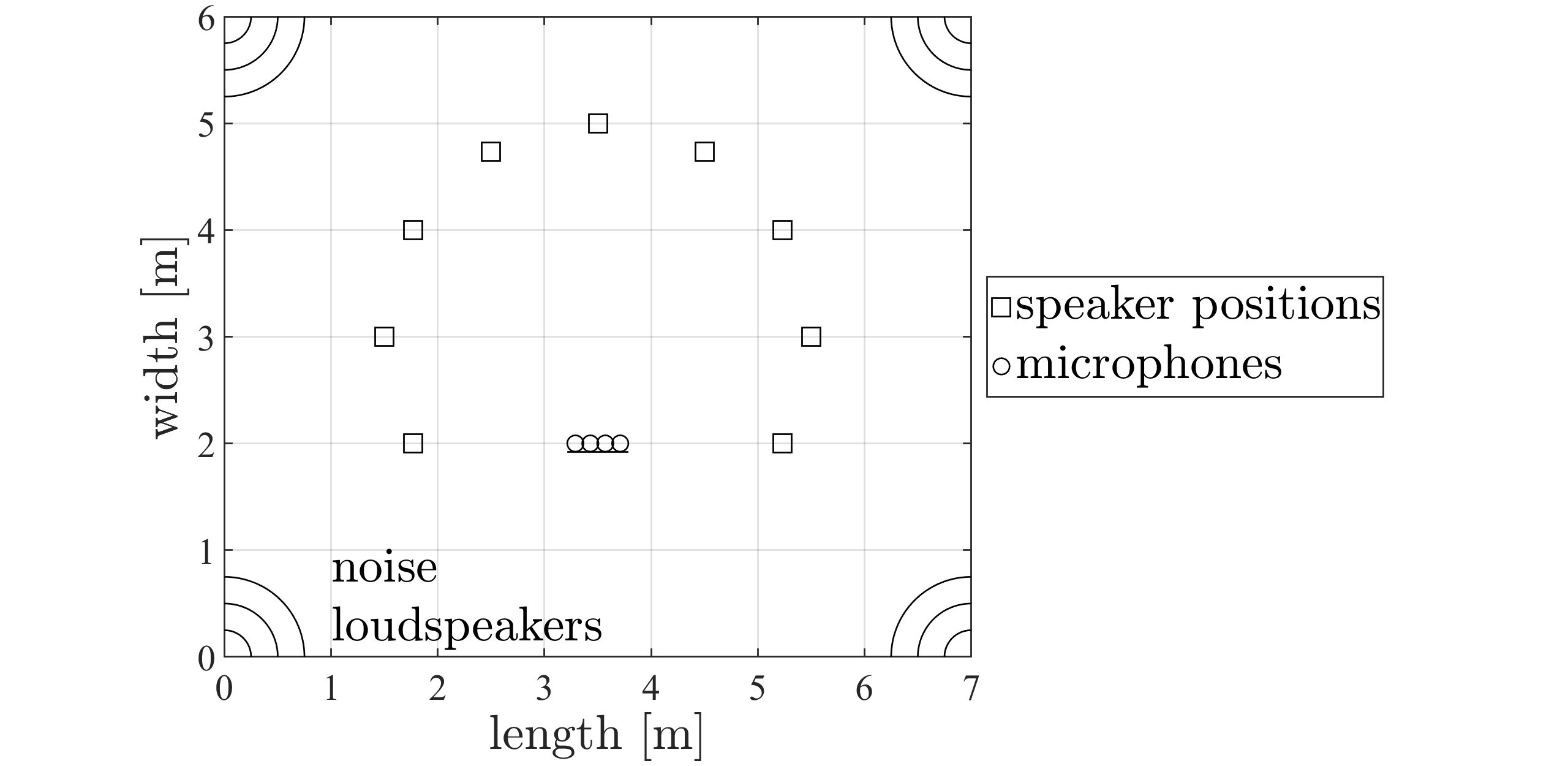
Figure 2: Acoustic setup with 9 speaker positions, a linear microphone array with 4 microphones and background noise.

The LCMV beamformer and RTF estimation is performed within an STFT framework with a frame length of 3200 samples (corresponding to $200\text{\,}\mathrm{ms}$), a frame shift of 800 samples (corresponding to $50\text{\,}\mathrm{ms}$) and a square-root-Hann window for analysis and synthesis. The scaling factor of the interfering speaker in (5) was set to $\delta=$-40\text{\,}\mathrm{dB}$$. The noise covariance matrix $\mathbf{R}_{\mathbf{n}}$ and the undesired covariance matrix $\mathbf{R}_{\mathbf{v},2}$ were estimated using the sample covariance matrix method in the noise-only and the single-speaker segment, respectively. The RTF vector $\mathbf{g}$ of the interfering speaker was estimated by CW in the single-speaker segment as described in Section 3.1.

The performance of the LCMV beamformer is evaluated in terms of the broadband signal-to-interferer-and-noise ratio (SINR) improvement for each microphone as reference ($r\in\{1,\ldots,M\}$), i.e.,

$$\Delta\mathrm{SINR}_{r}=10\cdot\log_{10}\left(\frac{\sum_{n}\left\lvert x_{r,n}^{\mathrm{out}}\right\rvert^{2}}{\sum_{n}\left\lvert v_{r,n}^{\mathrm{out}}\right\rvert^{2}}\right)-10\cdot\log_{10}\left(\frac{\sum_{n}\left\lvert x_{r,n}^{\mathrm{in}}\right\rvert^{2}}{\sum_{n}\left\lvert v_{r,n}^{\mathrm{in}}\right\rvert^{2}}\right),$$ (25)

where $n$ denotes the sample index, $x_{r,n}^{\mathrm{in}}$ and $v_{r,n}^{\mathrm{in}}$ denote the time-domain target speaker component and the undesired component (sum of interfering speaker and noise) in the $r$-th microphone signal, respectively, and $x_{r,n}^{\mathrm{out}}$ and $v_{r,n}^{\mathrm{out}}$ denote the shadow-filtered versions of $x_{r,n}^{\mathrm{in}}$ and $v_{r,n}^{\mathrm{in}}$ using the LCMV beamformer in (6).

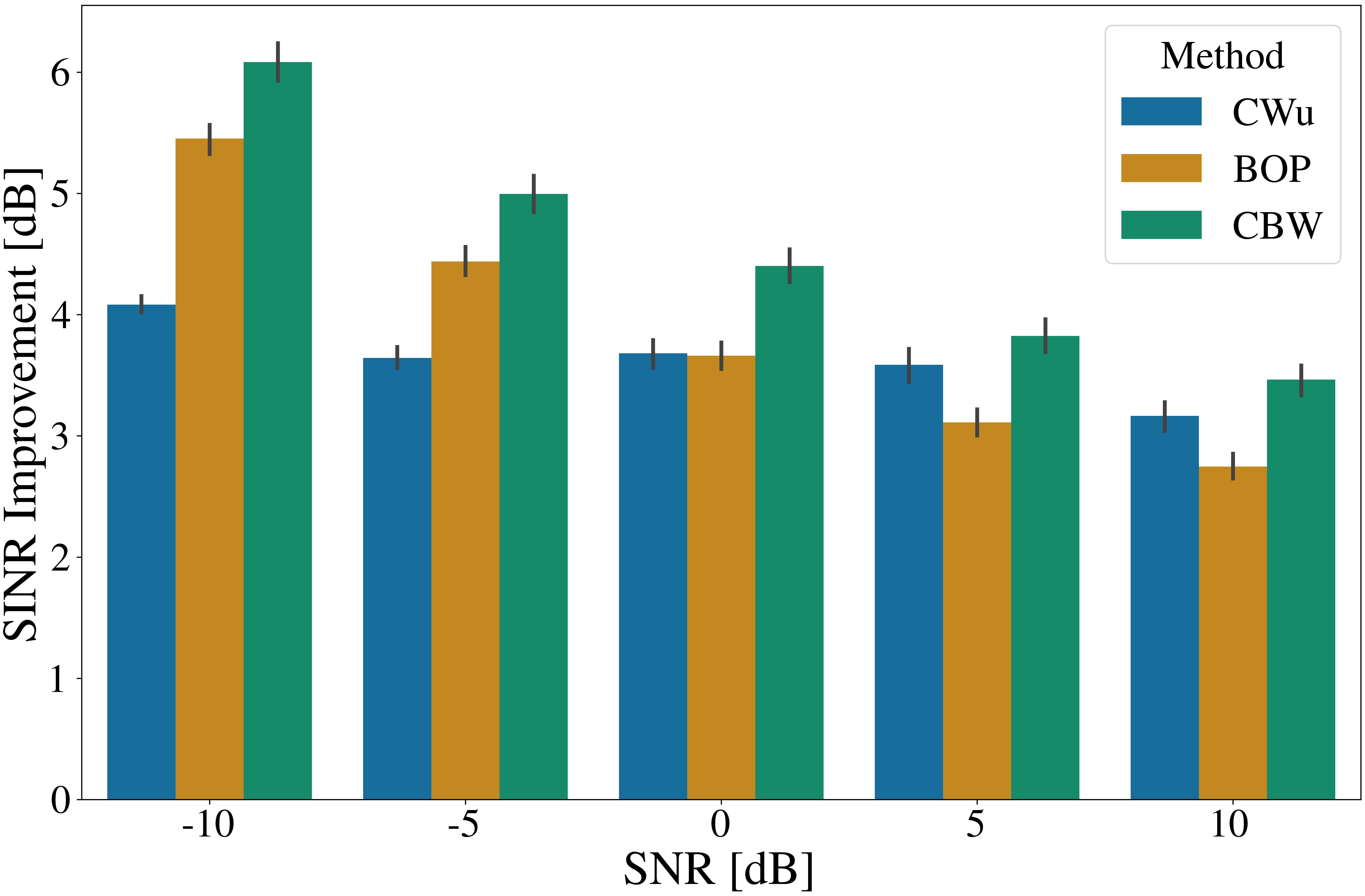
Figure 3: SINR improvement (average and standard deviation) for the considered RTF vector estimation methods (CWu, BOP, CBW) for different SNRs.

6.2 Results

For different SNRs, Figure 3 depicts the SINR improvement of the LCMV beamformer for the considered RTF vector estimation methods of the target speaker. Results were averaged over 72 non-collocated combinations of target and interferer position and 5 different broadband SIRs between $\left[$-10\text{\,}\mathrm{dB}$,$10\text{\,}\mathrm{dB}$\right]$ with an increment of $5\text{\,}\mathrm{dB}$. Results were also averaged over the choice of the reference microphone $m\in\{1,\ldots,M\}$. For all three methods, the SINR improvement increases for lower input SNRs, which can be explained by the larger potential improvement in conditions with more noise. For all considered SNRs, the CWu method yields an SINR improvement between $3\text{\,}\mathrm{d}\mathrm{B}$ and $4\text{\,}\mathrm{d}\mathrm{B}$. The BOP method outperforms the CWu method at low input SNRs, but yields a lower performance at high input SNRs. It can be observed that the proposed CBW method outperforms both conventional methods for all input SNRs, e.g., achieving an average SINR improvement of $6\text{\,}\mathrm{dB}$ for in the $-10\text{\,}\mathrm{dB}$ SNR condition.

7 Conclusion

In this paper, we proposed a covariance blocking and whitening (CBW) method to perform RTF vector estimation of the second speaker in a dual-speaker scenario with background noise, where the speakers activate successively. In contrast to the conventional methods (CWu and BOP), the CBW method uses an estimate of the RTF vector of the first speaker to block the first speaker before noise whitening. When using the estimated RTF vectors of both speakers in an LCMV beamformer, simulation results demonstrate that the proposed CBW method outperforms the conventional BOP and covariance whitening methods in terms of SINR improvement. In future work we aim at investigating different combinations of blocking and noise handling, e.g., also introduce noise handling to the BOP method.

References

- [1] R. Beutelmann and T. Brand, “Prediction of speech intelligibility in spatial noise and reverberation for normal-hearing and hearing-impaired listeners,” The Journal of the Acoustical Society of America, vol. 120, no. 1, pp. 331–342, Jul. 2006.
- [2] B. D. Van Veen and K. M. Buckley, “Beamforming: a versatile approach to spatial filtering,” IEEE ASSP Magazine, vol. 5, no. 2, pp. 4–24, Apr. 1988.
- [3] S. Doclo, W. Kellermann, S. Makino, and S. E. Nordholm, “Multichannel Signal Enhancement Algorithms for Assisted Listening Devices: Exploiting spatial diversity using multiple microphones,” IEEE Signal Processing Magazine, vol. 32, no. 2, pp. 18–30, Mar. 2015.
- [4] S. Gannot, E. Vincent, S. Markovich-Golan, and A. Ozerov, “A Consolidated Perspective on Multimicrophone Speech Enhancement and Source Separation,” IEEE/ACM Trans. on Audio, Speech, and Language Processing, vol. 25, no. 4, pp. 692–730, Apr. 2017.
- [5] E. Hadad, S. Doclo, and S. Gannot, “The Binaural LCMV Beamformer and its Performance Analysis,” IEEE/ACM Trans. on Audio, Speech, and Language Processing, vol. 24, no. 3, pp. 543–558, Mar. 2016.
- [6] N. Gößling, D. Marquardt, I. Merks, T. Zhang, and S. Doclo, “Optimal binaural LCMV beamforming in complex acoustic scenarios: Theoretical and practical insights,” in Proc. International Workshop on Acoustic Signal Enhancement, Tokyo, Japan, 2018, pp. 381–385.
- [7] J. Zhang, A. I. Koutrouvelis, R. Heusdens, and R. C. Hendriks, “Distributed rate-constrained LCMV beamforming,” IEEE Signal Processing Letters, vol. 26, no. 5, pp. 675–679, 2019.
- [8] S. Gannot, D. Burshtein, and E. Weinstein, “Signal enhancement using beamforming and nonstationarity with applications to speech,” IEEE Trans. on Signal Processing, vol. 49, no. 8, pp. 1614–1626, Aug. 2001.
- [9] I. Cohen, “Relative transfer function identification using speech signals,” IEEE Trans. on Speech and Audio Processing, vol. 12, no. 5, pp. 451–459, 2004.
- [10] E. Warsitz and R. Haeb-Umbach, “Blind acoustic beamforming based on generalized eigenvalue decomposition,” IEEE Trans. on Audio, Speech, and Language Processing, vol. 15, no. 5, pp. 1529–1539, 2007.
- [11] S. Markovich, S. Gannot, and I. Cohen, “Multichannel Eigenspace Beamforming in a Reverberant Noisy Environment With Multiple Interfering Speech Signals,” IEEE Trans. on Audio, Speech, and Language Processing, vol. 17, no. 6, pp. 1071–1086, Aug. 2009.
- [12] R. Serizel, M. Moonen, B. Van Dijk, and J. Wouters, “Low-rank Approximation Based Multichannel Wiener Filter Algorithms for Noise Reduction with Application in Cochlear Implants,” IEEE/ACM Trans. on Audio, Speech, and Language Processing, vol. 22, no. 4, pp. 785–799, Apr. 2014.
- [13] R. Varzandeh, M. Taseska, and E. A. Habets, “An iterative multichannel subspace-based covariance subtraction method for relative transfer function estimation,” in Proc. Hands-free Speech Communications and Microphone Arrays, 2017, pp. 11–15.
- [14] S. Markovich-Golan, S. Gannot, and W. Kellermann, “Performance analysis of the covariance-whitening and the covariance-subtraction methods for estimating the relative transfer function,” in Proc. European Signal Processing Conference, Rome, Italy, Sep. 2018, pp. 2499–2503.
- [15] A. Brendel, J. Zeitler, and W. Kellermann, “Manifold learning-supported estimation of relative transfer functions for spatial filtering,” in Proc. International Conference on Acoustics, Speech and Signal Processing, Singapore, 2022, pp. 8792–8796.
- [16] M. Tammen, S. Doclo, and I. Kodrasi, “Joint estimation of RETF vector and power spectral densities for speech enhancement based on alternating least squares,” in Proc. International Conference on Acoustics, Speech and Signal Processing, Brighton, UK, 2019, pp. 795–799.
- [17] C. Li, J. Martinez, and R. C. Hendriks, “Joint maximum likelihood estimation of microphone array parameters for a reverberant single source scenario,” IEEE/ACM Trans. on Audio, Speech, and Language Processing, vol. 31, pp. 695–705, 2023.
- [18] B. Schwartz, S. Gannot, and E. A. Habets, “Two model-based em algorithms for blind source separation in noisy environments,” IEEE/ACM Transactions on Audio, Speech, and Language Processing, vol. 25, no. 11, pp. 2209–2222, 2017.
- [19] A. I. Koutrouvelis, R. C. Hendriks, R. Heusdens, and J. Jensen, “Robust joint estimation of multimicrophone signal model parameters,” IEEE/ACM Trans. on Audio, Speech, and Language Processing, vol. 27, no. 7, pp. 1136–1150, 2019.
- [20] C. Li, J. Martinez, and R. C. Hendriks, “Low complex accurate multi-source RTF estimation,” in Proc. International Conference on Acoustics, Speech and Signal Processing, Singapore, 2022, pp. 4953–4957.
- [21] T. Dietzen, S. Doclo, M. Moonen, and T. van Waterschoot, “Square root-based multi-source early PSD estimation and recursive RETF update in reverberant environments by means of the orthogonal Procrustes problem,” IEEE/ACM Trans. on Audio, Speech, and Language Processing, vol. 28, pp. 755–769, 2020.
- [22] D. Cherkassky and S. Gannot, “Successive Relative Transfer Function Identification Using Blind Oblique Projection,” IEEE/ACM Trans. on Audio, Speech, and Language Processing, vol. 28, pp. 474–486, 2020.
- [23] Y. Avargel and I. Cohen, “On Multiplicative Transfer Function Approximation in the Short-Time Fourier Transform Domain,” IEEE Signal Processing Letters, vol. 14, no. 5, pp. 337–340, May 2007.
- [24] R. Behrens and L. Scharf, “Signal processing applications of oblique projection operators,” IEEE Trans. on Signal Processing, vol. 42, no. 6, pp. 1413–1424, Jun. 1994.
- [25] J. Nocedal and S. J. Wright, Numerical optimization. Springer, 1999.
- [26] The MathWorks, Inc., Optimization Toolbox User’s Guide, The MathWorks, Inc., 2023.