Electron EDM and LFV decays in the light of
Muon $(g-2)_{\mu}$ with U(2) flavor symmetry

1 Introduction

The electric and magnetic dipole moments of the electron and the muon are low-energy probes of New Physics (NP) beyond the Standard Model (SM). Recently, the muon $(g-2)_{\mu}$ experiment at Fermilab reported a new measurement of the muon magnetic anomaly using data collected in 2019 (Run-2) and 2020 (Run-3) [1]. Improvements of the analysis and run condition lead to more than a factor of two reduction in the systematic uncertainties, which is compared with the E989 experiment at Fermilab [2] and the previous BNL result [3]. This result indicates the discrepancy of $5.1\,\sigma$ with the SM prediction by "Muon $g-2$ Theory Initiative" [4] (see also [5, 6, 7, 8, 9, 10, 11, 12, 13, 14]).

While there is a debatable point on the precise value of the SM prediction. The problem is the contribution of the hadronic vacuum polarization (HVP). The current situation is complicated. The CMD-3 collaboration [15] released results on the cross section that disagree at the $(2.5-5)\sigma$ level with all previous measurements including those from the previous CMD-2 collaborations. The origin of this discrepancy is currently unknown. The BMW collaboration published the first complete lattice-QCD result with subpercent precision [16]. Their result is closer to the experimental average ($1.7\sigma$ tension for no NP in the muon $(g-2)_{\mu}$). Further studies are underway to clarify these theoretical differences. The white paper (SM prediction) is expected to be updated including the HVP problem in 2024.

If the muon $(g-2)_{\mu}$ anomaly comes from NP, it possibly appears in other observables of the charged lepton sector. The interesting one is the electric dipole moments (EDM) of the electron. In this year, the JILA group has reported a new upper-bound on the electron EDM, which is $|d_{e}|<4.1\times 10^{-30}\rm e\,cm\,(90\%\,{confidence})$, by using the $\rm{}^{18}Hf^{19}f^{+}$ ions trapped by the rotating electric field [17]. It overcame the latest ACME collaboration result obtained in 2018 [18]. Precise measurements of the electron EDM will be rapidly being updated. The future sensitivity at ACME $\rm I\hskip-1.13791ptI\hskip-1.13791ptI$ is expected to be $|d_{e}|<0.3\times 10^{-30}\,\text{e\,cm}$ [19, 20]. In contrast, the present upper-bound of the muon [21] and tauon EDM’s [22, 23, 24] are not so tight.

The lepton flavor violation (LFV) is also possible NP phenomena of the charged leptons. The tightest constraint for LFV is the branching ratio of the $\mu\to e\gamma$ decay. The experimental bound is $\mathcal{B}({\mu^{+}\to e^{+}\gamma})<4.2\times 10^{-13}$ in the MEG experiment [25]. On the other hands, the present upper-bounds of $\mathcal{B}\,({\tau\to\mu\gamma})$ and $\mathcal{B}\,({\tau\to e\gamma})$ are $4.4~{}\times~{}10^{-8}$ and $3.3~{}\times~{}10^{-8}$ [26, 27], respectively.

Comprehensive studies of the electric and magnetic dipole moments of leptons are given in the SM Effective Field Theory (SMEFT) [28, 29, 30], i.e., under the hypothesis of new degrees of freedom above the electroweak scale [31, 32, 33, 34]. The phenomenological discussion of NP has presented taking the anomaly of the muon $(g-2)_{\mu}$ and the LFV bound in the SMEFT with imposing $U(2)_{L_{L}}\otimes U(2)_{E_{R}}$ flavor symmetry [35], which is the corresponding subgroup acting only on the first two (light) families [36, 37, 38]. Since this flavor symmetry reduces the number of independent parameters of the flavor sector [39, 40], we can expect the interplay among possible NP evidence in the observables of different flavors, which is independent of details of NP. Thus, the SMEFT with flavor symmetry can probe NP without discussing its dynamics in the flavor space.

We have already studied the interplay of NP among the muon $(g-2)_{\mu}$, the electron EDM and the $\mu\to e\gamma$ decay in the modular symmetry of flavors [41, 42], which is realized in the context of string effective field theory [43] (see also [44]). The obtained result depends on the modular weights of the charged leptons and the relevant discrete symmetry, considerably. Therefore, more general discussions are required to confirm the role of flavor symmetry for the NP search without depending on details of the flavor model.

There are many possible discrete symmetries for the leptons flavor mixing [45, 46, 47, 48, 49, 50, 51, 52, 53, 54, 55]. Some of them are subgroups of continuous groups [48]. On the other hand, the NP analysis of SMEFT has been performed attractively by imposing the flavor symmetry of continuous group, especially $U(2)$ [39, 40]. We also adopt the $U(2)$ flavor symmetry for discussing the dipole operator of leptons to investigate NP [35]. In this paper, we present numerical discussions of the interplay of NP in the light of recent data of the muon $(g-2)_{\mu}$ and the electron EDM by taking $U(2)_{L_{L}}\otimes U(2)_{E_{R}}$ flavor symmetry of the charged leptons. Since we discuss the electron EDM, we analyze NP in the three family space of $U(2)_{L_{L}}\otimes U(2)_{E_{R}}$ flavor symmetry to take into account of possible CP violating phases. It is remarked that the third-family contributes significantly to the $\mu\to e\gamma$ decay and the electron EDM.

In addition to the muon $(g-2)_{\mu}$ and the electron EDM, we also study $(g-2)_{e,\tau}$ of the electron and tauon, and EDM of the muon and tauon as well as LFV processes $\tau\to e\gamma$ and $\tau\to\mu\gamma$.

The paper is organized as follows. In section 2, we discuss the experimental constraints for Wilson coefficients of the leptonic dipole operator. In section 3, we present our framework of the $U(2)$ flavor model. In section 4, numerical discussions are presented. The summary and discussion are devoted to section 5. In Appendix A, the experimental constraints of the relevant Wilson coefficients of the leptonic dipole operator are presented. In Appendix B, the $3\times 3$ Yukawa matrices, $YY^{\dagger}$ and $Y^{\dagger}Y$, are given explicitly.

2 Constraints of Wilson coefficients of the dipole operator

2.1 Input experimental data

The combined result from the E989 experiment at Fermilab  [1, 2] and the E821 experiment at BNL [3] on $a_{\mu}=(g-2)_{\mu}/2$, together with the SM prediction $a_{\mu}^{\mathrm{SM}}$ in [4], implies

$$\Delta a_{\mu}=a_{\mu}^{\mathrm{Exp}}-a_{\mu}^{\mathrm{SM}}=\left(249\pm 49\right)\times 10^{-11}~{}.$$ (1)

We suppose that the contribution of NP appears in $\Delta a_{\mu}$.

However, the precise value of the SM prediction of HVP is still unclear. Further studies will clarify the theoretical differences. If $\Delta a_{\mu}$ is significantly lower, less than or of order $1\,\sigma$, one may obtain somewhat loose bound in phenomenological studies of NP [56]. In our study, we take a following reference value (the discrepancy of $5.1\,\sigma$ with the SM prediction) as the input in our numerical analysis:

$$\Delta a_{\mu} =249\times 10^{-11}\,.$$ (2)

We will comment on our result in the case that the discrepancy with the SM prediction is reduced in section 5.

We also input the upper-bound of the electron EDM by the JILA group [17]:

$$|{d_{e}}|<4.1\times 10^{-30}\,\rm e\,cm=6.3\times 10^{-14}\,TeV^{-1}\,.$$ (3)

On the other hand, the upper-bound of muon EDM is [21]:

$$|{d_{\mu}}|<1.8\times 10^{-19}\,\rm e\,cm=2.76\times 10^{-3}\,TeV^{-1}\,.$$ (4)

The tauon EDM can be evaluated through the measurement of CP-violating correlations in tauon-pair production such as $e^{+}e^{-}\to\tau^{+}\tau^{-}$ [22] (see also [23]). The present upper-bound on the tauon EDM $d_{\tau}$ is given as: [24]:

$$-1.85\times 10^{-17}{\rm e\,cm}<{\rm Re}\,d_{\tau}<0.61\times 10^{-17}{\rm e\,cm},\ \ -1.03\times 10^{-17}{\rm e\,cm}<{\rm Im}\,d_{\tau}<0.23\times 10^{-17}{\rm e\,cm}.$$ (5)

Taking the bound of ${\rm Re}\,d_{\tau}$, we have

$$|d_{\tau}|<1.85\times 10^{-17}{\rm e\,cm}=2.84\,{\rm TeV}^{-1}\,.$$ (6)

The experimental upper-bound for the branching ratio of $\mu\to e\gamma$ is [25]:

$$\mathcal{B}({\mu^{+}\to e^{+}\gamma})<4.2\times 10^{-13}\,.$$ (7)

We also take account of the upper-bound for LFV comes from the branching ratios of $\tau\to\mu\gamma$ and $\tau\to e\gamma$ [26, 27] :

$$\mathcal{B}({\tau\to\mu\gamma})<4.2\times 10^{-8}\,,\quad\qquad\mathcal{B}({\tau\to e\gamma})<3.3\times 10^{-8}\,.$$ (8)

These input data are converted into the magnitudes of the Wilson coefficients of the leptonic dipole operator in the next subsection.

2.2 Wilson coefficients of the leptonic dipole operator

We make the assumption that NP is heavy and can be given by the SMEFT Lagrangian. Let us focus on the dipole operators of leptons and their Wilson coefficients at the weak scale as:

$$\mathcal{O}_{\underset{LR}{e\gamma}}=\frac{v}{\sqrt{2}}\overline{E}_{L}\sigma^{\mu\nu}E_{R}F_{\mu\nu}\,,\qquad\qquad\mathcal{C}_{\underset{LR}{e\gamma}}^{\prime}=\begin{pmatrix}\mathcal{C}_{\underset{ee}{e\gamma}}^{\prime}&\mathcal{C}_{\underset{e\mu}{e\gamma}}^{\prime}&\mathcal{C}_{\underset{e\tau}{e\gamma}}^{\prime}\\ \mathcal{C}_{\underset{\mu e}{e\gamma}}^{\prime}&\mathcal{C}_{\underset{\mu\mu}{e\gamma}}^{\prime}&\mathcal{C}_{\underset{\mu\tau}{e\gamma}}^{\prime}\\ \mathcal{C}_{\underset{\tau e}{e\gamma}}^{\prime}&\mathcal{C}_{\underset{\tau\mu}{e\gamma}}^{\prime}&\mathcal{C}_{\underset{\tau\tau}{e\gamma}}^{\prime}\\ \end{pmatrix}\,,$$

$$\mathcal{O}_{\underset{RL}{e\gamma}}=\frac{v}{\sqrt{2}}\overline{E}_{R}\sigma^{\mu\nu}E_{L}F_{\mu\nu}\,,\qquad\qquad\mathcal{C}_{\underset{RL}{e\gamma}}^{\prime}=\mathcal{C}_{\underset{LR}{e\gamma}}^{\prime\,\dagger}\,,$$ (9)

where $E_{L}$ and $E_{R}$ denote three flavors of the left-handed and right-handed leptons, respectively, and $v$ denotes the vacuum expectation value (VEV) of the Higgs field $H$. The prime of the Wilson coefficient indicates the flavor basis corresponding to the mass-eigenstate basis of the charged leptons. The relevant effective Lagrangian is written as:

$$\mathcal{L}_{\rm dipole}=\frac{1}{\Lambda^{2}}\,\left(\mathcal{C}_{\underset{LR}{e\gamma}}^{\prime}\mathcal{O}_{\underset{LR}{e\gamma}}+\mathcal{C}_{\underset{RL}{e\gamma}}^{\prime}\mathcal{O}_{\underset{RL}{e\gamma}}\right)\,,$$ (10)

where $\Lambda$ is a certain mass scale of NP in the effective theory. Here the Wilson coefficient is understood to be evaluated at the weak scale (we neglect the small effect of running below the weak scale) .

Inputting the value in Eq. (2), the Wilson coefficient is obtained as[35] (see Appendix A):

$$\frac{1}{\Lambda^{2}}\text{Re}\ [\mathcal{C}_{\underset{\mu\mu}{e\gamma}}^{\prime}]=1.0\times 10^{-5}\,\mathrm{TeV}^{-2}\,.$$ (11)

The LFV process $\mu\to e\gamma$ gives us more severe constraint for the Wilson coefficient by the experimental data in Eq. (7). The upper-bound is obtained [35] (see Appendix A):

$$\frac{1}{\Lambda^{2}}|\mathcal{C}_{\underset{e\mu(\mu e)}{e\gamma}}^{\prime}|<2.1\times 10^{-10}\,\mathrm{TeV}^{-2}\,.$$ (12)

Taking into account Eqs. (11) and (12), one has the ratio [35] :

$$\left|\frac{\mathcal{C}_{\underset{e\mu(\mu e)}{e\gamma}}^{\prime}}{\mathcal{C}_{\underset{\mu\mu}{e\gamma}}^{\prime}}\right|<2.1\times 10^{-5}\,.$$ (13)

Thus, the magnitude of $\mathcal{C}_{\underset{e\mu(\mu e)}{e\gamma}}^{\prime}$ is much suppressed compared with $\mathcal{C}_{\underset{\mu\mu}{e\gamma}}^{\prime}$. This gives the severe constraint for parameters of the flavor model.

The $\tau\to\mu\gamma$ process also gives us another constraint for the Wilson coefficient by the experimental data in Eq. (8). The upper-bounds are obtained as seen in Appendix A:

$$\frac{1}{\Lambda^{2}}|\mathcal{C}_{\underset{\mu\tau(\tau\mu)}{e\gamma}}^{\prime}|<2.65\times 10^{-6}\,\mathrm{TeV}^{-2}\,,\qquad\frac{1}{\Lambda^{2}}|\mathcal{C}_{\underset{e\tau(\tau e)}{e\gamma}}^{\prime}|<2.35\times 10^{-6}\,\mathrm{TeV}^{-2}.$$ (14)

The electron EDM, $d_{e}$ is defined in the operator:

$$\mathcal{O}_{\mathrm{edm}}=-\frac{i}{2}\,d_{e}(\mu)\,\overline{e}\sigma^{\mu\nu}\gamma_{5}eF_{\mu\nu}\,,$$ (15)

where $d_{e}=d_{e}(\mu=m_{e})$. Therefore, the electron EDM is extracted from the effective Lagrangian

$$\mathcal{L}_{\rm EDM}=\frac{1}{\Lambda^{2}}\mathcal{C}_{\underset{ee}{e\gamma}}^{\prime}\mathcal{O}_{\underset{LR}{e\gamma}}=\frac{1}{\Lambda^{2}}\mathcal{C}_{\underset{ee}{e\gamma}}^{\prime}\frac{v}{\sqrt{2}}\overline{e}_{L}\sigma^{\mu\nu}e_{R}F_{\mu\nu}\,,$$ (16)

which leads to

$$d_{e}=-\sqrt{2}\,\frac{v}{\Lambda^{2}}\,{\rm Im}\,[\mathcal{C}_{\underset{ee}{e\gamma}}^{\prime}]\,,$$ (17)

at tree level, where the small effect of running below the electroweak scale is neglected.

Inputting the experimental upper-bound of the electron EDM in Eq. (3) [17], we obtain the constraint of the Wilson coefficient:

$$\frac{1}{\Lambda^{2}}{\mathrm{Im}}\,[\mathcal{C}_{\underset{ee}{e\gamma}}^{\prime}]<1.8\times 10^{-13}\,\mathrm{TeV^{-2}}\,.$$ (18)

On the other hand, the experimental upper-bound of the muon EDM in Eq. (4) gives:

$$\frac{1}{\Lambda^{2}}{\mathrm{Im}}\,[\mathcal{C}_{\underset{\mu\mu}{e\gamma}}^{\prime}]<7.9\times 10^{-3}\,\mathrm{TeV^{-2}}\,.$$ (19)

Observables	Exp.$-$ SM / upper bound	Wilson Coef. in $1/\Lambda^{2}\ [\mathrm{TeV}^{-2}]$
$\Delta a_{\mu}$	$249\times 10^{-11}$[1, 2, 3]	$\text{Re}\ [\mathcal{C}_{\underset{\mu\mu}{e\gamma}}^{\prime}]=1.0\times 10^{-5}$
$\mathcal{B}({\mu^{+}\to e^{+}\gamma})$	$<4.2\times 10^{-13}$ [25]	$|\mathcal{C}_{\underset{e\mu(\mu e)}{e\gamma}}^{\prime}|<2.1\times 10^{-10}$
$\mathcal{B}({\tau\to\mu\gamma})$	$<4.2\times 10^{-8}$ [26, 27]	$|\mathcal{C}_{\underset{\mu\tau(\tau\mu)}{e\gamma}}^{\prime}|<2.65\times 10^{-6}$
$\mathcal{B}({\tau\to e\gamma})$	$<3.3\times 10^{-8}$ [26, 27]	$|\mathcal{C}_{\underset{e\tau(\tau e)}{e\gamma}}^{\prime}|<2.35\times 10^{-6}$
$|d_{e}|$	$<4.1\times 10^{-30}\,\rm e\,cm$ [17]	$\text{Im}\ [\mathcal{C}_{\underset{ee}{e\gamma}}^{\prime}]<1.8\times 10^{-13}$
$|d_{\mu}|$	$<1.80\times 10^{-19}\,\rm e\,cm$[21]	$\text{Im}\ [\mathcal{C}_{\underset{\mu\mu}{e\gamma}}^{\prime}]<7.9\times 10^{-3}$
$|d_{\tau}|$	$<1.85\times 10^{-17}\,\rm e\,cm$ [22]	$\text{Im}\ [\mathcal{C}_{\underset{\tau\tau}{e\gamma}}^{\prime}]<8.2\times 10^{-1}$

Table 1: Relevant observables and the corresponding values of Wilson coefficients, which are presented in $1/\Lambda^{2}\ (\mathrm{TeV}^{-2})$ unit.

The upper-bound of the tauon EDM in Eq. (6) also gives:

$$\frac{1}{\Lambda^{2}}{\mathrm{Im}}\,[\mathcal{C}_{\underset{\tau\tau}{e\gamma}}^{\prime}]<8.2\times 10^{-1}\,\mathrm{TeV^{-2}}\,.$$ (20)

By using these bounds of Wilson coefficients, we analyze the $U(2)$ flavor model in the next section. These data are listed in Table 1.

3 U(2) flavor model

3.1 Flavor structure of Yukawa and dipole operator in charged leptons

In the lepton sector, we impose $U(2)_{L_{L}}\otimes U(2)_{E_{R}}$ flavor symmetry, which is the corresponding subgroup acting only on the first two light families. The minimal set of the breaking terms, which are so called spurions, are

$$V_{\ell}\sim(\bf{2,\,1})\,,\qquad\Delta_{e}\sim(\bf{2,\,\bar{2}})\,.$$ (21)

The two suprions can be parameterized by

$$V_{\ell}=\begin{pmatrix}0\\ {\epsilon_{\ell}}\,\end{pmatrix},\qquad\Delta_{e}=O_{e}^{T}\ \begin{pmatrix}\delta^{\prime}_{e}&0\\ 0&\delta_{e}\\ \end{pmatrix}\,,\qquad O_{e}=\begin{pmatrix}c_{e}&s_{e}\\ -s_{e}&c_{e}\\ \end{pmatrix}\,,$$ (22)

where $\delta^{\prime}_{e}$, $\delta_{e}$ and $\epsilon_{\ell}$ are taken to be real without loss of generality, while $c_{e}$ and $s_{e}$ denote $\cos\theta_{e}$ and $\sin\theta_{e}$, respectively. By using the spurions in Eq. (22), the $3\times 3$ Yukawa coupling of leptons $Y$ is written in the right-left (LR) convention at order ${\cal O}(V_{\ell}^{2}\Delta_{e})$ and ${\cal O}(V_{\ell}^{3})$ of spurion couplings:

$$Y=\begin{pmatrix}C^{y}_{\Delta}(\Delta_{e})_{\alpha\beta}+C^{y}_{VV\Delta}(V_{\ell})_{\alpha}(V_{\ell}^{\dagger})_{\gamma}(\Delta_{e})_{\gamma\beta}&C^{y}_{V}(V_{\ell})_{\alpha}+C^{y}_{VVV}(V_{\ell})(V_{\ell}^{\dagger})(V_{\ell})_{\alpha}\\ C^{y}_{V\Delta}(V_{\ell}^{\dagger})_{\alpha}(\Delta_{e})_{\alpha\beta}&C^{y}+C^{y}_{VV}(V_{\ell}^{\dagger}V_{\ell})\end{pmatrix}_{LR}\,,$$ (23)

where $\alpha,\beta$ are the first or second component in Eq. (22). Taking suprion parameters in Eq. (22), the Yukawa matrix is written explicitly as:

$$Y=\begin{pmatrix}C^{y}_{\Delta}c_{e}\delta_{e}^{\prime}&-C^{y}_{\Delta}s_{e}\delta_{e}&0\\ s_{e}\delta_{e}^{\prime}(C^{y}_{\Delta}+C^{n}_{VV\Delta}\epsilon_{\ell}^{2})&c_{e}\delta_{e}(C^{y}_{\Delta}+C^{y}_{VV\Delta}\epsilon_{\ell}^{2})&(C^{y}_{V}\epsilon_{\ell}+C^{y}_{VVV}\epsilon_{\ell}^{3})\\ C^{y}_{V\Delta}(s_{e}\epsilon_{\ell}\delta_{e}^{\prime})&C^{y}_{V\Delta}(c_{e}\epsilon_{\ell}\delta_{e})&C^{y}+C^{y}_{VV}\epsilon_{\ell}^{2}\end{pmatrix}_{LR}\,,$$ (24)

where $C^{y}$, $C^{y}_{\Delta}$, $C^{y}_{V}$, $C^{y}_{V\Delta}$, $C^{y}_{VV\Delta}$ and $C^{y}_{VVV}$ are complex parameters of order $1$.

The flavor structure of the leptonic dipole operator in Eq. (9) is given by $3\times 3$ matrix $X^{e\gamma}$. It is also given in terms of spurion couplings like in Eq. (23) as follows:

$$X^{e\gamma} =\begin{pmatrix}C^{e\gamma}_{\Delta}(\Delta_{e})_{\alpha\beta}+C^{e\gamma}_{VVV}(V_{\ell})_{\alpha}(V_{\ell}^{\dagger})_{\gamma}(\Delta_{e})_{\gamma\beta}&C^{e\gamma}_{V}(V_{\ell})_{\alpha}+C^{e\gamma}_{VVV}(V_{\ell})(V_{\ell}^{\dagger})(V_{\ell})_{\alpha}\\ C^{e\gamma}_{V\Delta}(V_{\ell}^{\dagger})_{\alpha}(\Delta_{e})_{\alpha\beta}&C^{e\gamma}+C^{e\gamma}_{VV}(V_{\ell}^{\dagger}V_{\ell})\end{pmatrix}_{LR}\,$$

$$=\begin{pmatrix}C^{e\gamma}_{\Delta}c_{e}\delta_{e}^{\prime}&-C^{e\gamma}_{\Delta}s_{e}\delta_{e}&0\\ s_{e}\delta_{e}^{\prime}(C^{e\gamma}_{\Delta}+C^{e\gamma}_{VV\Delta}\epsilon_{\ell}^{2})&c_{e}\delta_{e}(C^{e\gamma}_{\Delta}+C^{e\gamma}_{VV\Delta}\epsilon_{\ell}^{2})&(C^{e\gamma}_{V}\epsilon_{\ell}+C^{e\gamma}_{VVV}\epsilon_{\ell}^{3})\\ C^{e\gamma}_{V\Delta}(s_{e}\epsilon_{\ell}\delta_{e}^{\prime})&C^{e\gamma}_{V\Delta}(c_{e}\epsilon_{\ell}\delta_{e})&C^{e\gamma}+C^{e\gamma}_{VV}\epsilon_{\ell}^{2}\end{pmatrix}_{LR}\,,$$ (25)

where $C^{e\gamma}$, $C^{e\gamma}_{\Delta}$, $C^{e\gamma}_{V}$, $C^{e\gamma}_{V\Delta}$, $C^{e\gamma}_{VV\Delta}$ and $C^{e\gamma}_{VVV}$ are also complex parameters of order $1$. Since the Wilson coefficients in Eq. (9) are written in the mass-eigenstate basis of the charged leptons, the matrix $X^{e\gamma}$ in Eq.(25) should be transformed into the diagonal basis of $Y$ in Eq.(24).

The eigenvalues of Yukawa matrix $Y$ in Eq.(24) ($y_{e}\ll y_{\mu}\ll y_{\tau}$) are obtained by solving the eigenvalue equation. For the determinant and trace of $YY^{\dagger}$, one finds in the leading order:

$${\rm Det}\,[YY^{\dagger}]=y^{2}_{e}\,y^{2}_{\mu}\,y^{2}_{\tau}\simeq|C^{y}_{\Delta}|^{4}\,|C^{y}|^{2}\,c_{e}^{4}\,\delta_{\ell}^{2}\,{\delta^{\prime}_{\ell}}^{2}\,,$$

$${\rm Tr}\,[YY^{\dagger}]=y^{2}_{e}+y^{2}_{\mu}+y^{2}_{\tau}\simeq|C^{y}|^{2}\,,$$ (26)

where $\delta_{e}$ and $\delta^{\prime}_{e}$ are much smaller than $1$ to reproduce the charged lepton mass hierarchy. An expression for $y_{\mu}^{2}y_{\tau}^{2}$ is given by the determinant of the 2-3 submatrix:

$$y_{\mu}^{2}\,y_{\tau}^{2}\simeq|C^{y}_{\Delta}|^{2}\,|C^{y}|^{2}\,c_{e}^{2}\,\delta_{\ell}^{2}\,.$$ (27)

Then, one gets

$$y_{\tau}^{2}\simeq|C^{y}|^{2}\,,\qquad y_{\mu}^{2}\simeq|C^{y}_{\Delta}|^{2}c_{e}^{2}\,\delta_{\ell}^{2}\,,\qquad y_{e}^{2}\simeq|C^{y}_{\Delta}|^{2}c_{e}^{2}\,{\delta^{\prime}_{\ell}}^{2}\,,\qquad$$ (28)

which lead to

$$\frac{y_{e}^{2}}{y_{\mu}^{2}}\simeq\frac{{\delta^{\prime}_{\ell}}^{2}}{\delta_{\ell}^{2}}\,,\qquad\frac{y_{\mu}^{2}}{y_{\tau}^{2}}\simeq\frac{\delta_{\ell}^{2}}{|C^{y}_{\Delta}|^{2}}\,.$$ (29)

These ratio indicates $\delta_{\ell}\gg\delta^{\prime}_{\ell}$ to reproduce the Yukawa hierarchy of the charged leptons. Especially, ${y_{e}^{2}}/{y_{\mu}^{2}}$ is independent of other coefficients of order one. The parameters $\epsilon_{\ell}$ and $s_{e}$ are not constrained by the charged lepton mass spectrum.

The neutrino mass matrix was discussed in $U(2)$ and $U(3)$ flavor model [38]. Indeed, the large lepton mixing angles come from the neutrino mass matrix. However, we do not address details of neutrino mass matrix because its contribution to our result is negligibly small due to small neutrino masses.

We can presume the magnitudes of $s_{e}$ and $\epsilon_{\ell}$ from the CKM mixing angles of the quark sector. In our numerical analysis, we scan $s_{e}$ and $\epsilon_{\ell}$ as variant parameters without fixing in advance as:

$$s_{e}=0.01-0.1\,,\qquad\epsilon_{\ell}=0.01-0.1\,.$$ (30)

These ranges are set to be consistent with the viewpoint of quark sector in Refs.[38, 40].

3.2 Mass-eigenstate basis of the charged leptons

The Yukawa matrix $Y$ in Eq. (24) is diagonalized by the unitary transformation $U_{L}^{\dagger}YU_{R}$, where the unitary matrices are given in terms of $2\times 2$ orthogonal matrices and phase matrices:

$$U_{L}=P_{L23}U_{L23}P_{L13}U_{L13}P_{L12}U_{L12}\,,\qquad U_{R}=P_{R23}U_{R23}P_{R13}U_{R13}P_{R12}U_{R12}\,,$$ (31)

where the rotation matrices are

$$U_{12}=\begin{pmatrix}c_{12}&s_{12}&0\\ -s_{12}&c_{12}&0\\ 0&0&1\\ \end{pmatrix}\,,\qquad U_{13}=\begin{pmatrix}c_{13}&0&s_{13}\\ 0&1&0\\ -s_{13}&0&c_{13}\\ \end{pmatrix}\,,\qquad U_{23}=\begin{pmatrix}1&0&0\\ 0&c_{23}&s_{23}\\ 0&-s_{23}&c_{23}\\ \end{pmatrix}\,,$$ (32)

and phase matrices are

$$P_{12}=\begin{pmatrix}1&0&0\\ 0&e^{i\phi_{12}}&0\\ 0&0&1\\ \end{pmatrix}\,,\qquad P_{13}=\begin{pmatrix}1&0&0\\ 0&1&0\\ 0&0&e^{i\phi_{13}}\\ \end{pmatrix}\,,\qquad P_{23}=\begin{pmatrix}1&0&0\\ 0&1&0\\ 0&0&e^{i\phi_{23}}\\ \end{pmatrix}\,,$$ (33)

where notations $L$ and $R$ are omitted. The $s_{ij}$ and $\phi_{ij}$ are obtained approximately from $YY^{\dagger}$ or $Y^{\dagger}Y$ in Appendix B for the left-handed or the right-handed sector.

In the following expression, we take $C^{y}_{\Delta}$ to be real positive and $C^{y}$, $C^{y}_{V}$, $C^{y}_{VV\Delta}$ and $C^{y}_{VVV}$ to be complex without loss of generality. The mixing angles $s_{Lij}$ and $s_{Rij}$ are obtained approximately (see Appendix B). The mixing angles $s_{L12}$ and $s_{R12}$ are :

$$s_{L12}\simeq-\frac{s_{e}}{c_{e}}\left[1-\left|\frac{C^{y}_{VV\Delta}}{C^{y}_{\Delta}}\right|\epsilon_{\ell}^{2}\cos(\arg C^{y}_{VV\Delta})\right]\,,$$

$$s_{R12}\simeq 2\frac{s_{e}}{c_{e}}\frac{\delta^{\prime}_{e}}{\delta_{e}}\left[\cos(\arg C^{y}_{VV\Delta})+\left|\frac{C^{y}_{VV\Delta}}{2C^{y}_{\Delta}}\right|\epsilon_{\ell}^{2}\right]\left|\frac{C^{y}_{VV\Delta}}{C^{y}_{\Delta}}\right|\epsilon_{\ell}^{2}\,,$$ (34)

respectively. The phase $\phi_{L12}$ and $\phi_{R12}$ are:

$$\phi_{L12}\simeq-\left|\frac{C^{y}_{VV\Delta}}{C^{y}_{\Delta}}\right|\epsilon_{\ell}^{2}\sin(\arg C^{y}_{VV\Delta})\,,\qquad\phi_{R12}\simeq 0\,,$$ (35)

which are much smaller than $1$. The mixing angles $s_{L23}$ and $s_{R23}$ are rather simple in the leading order as:

$$s_{L23}\simeq\left|\frac{C^{y}_{V}}{C^{y}}\right|\epsilon_{\ell}\,,\qquad s_{R23}\simeq\left|\frac{C^{y\,*}_{\Delta}C^{y}_{V}+C^{y\,*}_{V\Delta}C^{y}}{C^{y\,2}}\right|c_{e}\delta_{e}\epsilon_{\ell}\,,$$ (36)

respectively. The phase $\phi_{L12}$ and $\phi_{R12}$ are:

$$\phi_{L23}\simeq\arg\frac{C^{y}_{V}}{C^{y}}\,,\qquad\phi_{R23}\simeq\arg\left[\frac{C^{y\,*}_{\Delta}C^{y}_{V}+C^{y\,*}_{V\Delta}C^{y}}{|C^{y}|^{2}}\right]\,,$$ (37)

which are of order $1$.

The mixing angles $s_{L13}$ and $s_{R13}$ are also simple in the leading order as:

$$s_{L13}\simeq\left|\frac{C^{y}_{\Delta}C^{y\,*}_{V\Delta}}{C^{y\,2}}\right|c_{e}s_{e}(\delta_{e}^{2}-{\delta^{\prime}_{e}}^{2})\epsilon_{\ell}\,,\qquad s_{R13}\simeq\left|\frac{C^{y\,*}_{\Delta}C^{y}_{V}+C^{y\,*}_{V\Delta}C^{y}}{C^{y\,2}}\right|s_{e}\delta^{\prime}_{e}\epsilon_{\ell}\,,$$ (38)

respectively. The phase $\phi_{L13}$ and $\phi_{R13}$ are:

$$\phi_{L13}\simeq\arg\frac{C^{y}_{\Delta}C^{y\,*}_{V\Delta}}{|C^{y}|^{2}}\,,\qquad\qquad\phi_{R13}\simeq 0\,.$$ (39)

It is noticed that the $(1,3)$ and $(2,3)$ components of $(Y^{\dagger}Y)_{RR}$ have the same phase as seen in Eq.(65). Therefore, the phase matrix $P_{R23}$ removes phases of both $(1,3)$ and $(2,3)$ components, that is, $\phi_{R13}\simeq 0$ is derived.

In mass-eigenstate basis, the matrix $X^{e\gamma}$ in Eq. (25) is transformed by the unitary matrix in Eq. (31) as $U_{L}^{\dagger}X^{e\gamma}U_{R}$, whose elements correspond to the Wilson coefficients of Eq. (9). Those are given as:

$$\mathcal{C}_{\underset{ee}{e\gamma}}^{\prime}=[U_{L}^{{\dagger}}X^{e\gamma}U_{R}]_{11}\simeq|C^{e\gamma}_{\Delta}|\delta_{e}^{\prime}\left[\frac{1}{c_{e}}+\frac{s_{e}^{2}}{c_{e}}\epsilon_{\ell}^{2}\left(\frac{C^{e\gamma}_{VV\Delta}}{C^{e\gamma}_{\Delta}}-\frac{C^{y}_{VV\Delta}}{C^{y}_{\Delta}}\right)\right]+\delta_{e}^{\prime}\frac{s_{e}^{2}}{c_{e}}\epsilon_{\ell}^{2}\,C_{3rd}\,,$$

$$\mathcal{C}_{\underset{\mu\mu}{e\gamma}}^{\prime}=[U_{L}^{{\dagger}}X^{e\gamma}U_{R}]_{22}$$

$$\quad\ \simeq|C^{e\gamma}_{\Delta}|\delta_{e}\left[\frac{1}{c_{e}}+c_{e}\epsilon_{\ell}^{2}\left(\left|\frac{C^{e\gamma}_{VV\Delta}}{C^{e\gamma}_{\Delta}}\right|\cos{(\arg{C^{e\gamma}_{VV\Delta}})}-\left|\frac{C^{y}_{VV\Delta}}{C^{y}_{\Delta}}\right|\frac{s_{e}^{2}}{c_{e}^{2}}\cos{(\arg{C^{y}_{VV\Delta}})}\right)\right]$$

$$\quad\ +i|C^{e\gamma}_{\Delta}|c_{e}\delta_{e}\epsilon_{\ell}^{2}\left(\left|\frac{C^{e\gamma}_{VV\Delta}}{C^{e\gamma}_{\Delta}}\right|\sin{(\arg{C^{e\gamma}_{VV\Delta}})}-\left|\frac{C^{y}_{VV\Delta}}{C^{y}_{\Delta}}\right|\sin{(\arg{C^{y}_{VV\Delta}})}\right)+c_{e}\delta_{e}\epsilon_{\ell}^{2}\,C_{3rd}\,,$$

$$\mathcal{C}_{\underset{e\mu}{e\gamma}}^{\prime}=[U_{L}^{{\dagger}}X^{e\gamma}U_{R}]_{12}\simeq|C^{e\gamma}_{\Delta}|s_{e}\delta_{e}\epsilon_{\ell}^{2}\left(\frac{C^{e\gamma}_{VV\Delta}}{C^{e\gamma}_{\Delta}}-\frac{C^{y}_{VV\Delta}}{C^{y}_{\Delta}}\right)+s_{e}\delta_{e}\epsilon_{\ell}^{2}\,C_{3rd}\,,$$

$$\mathcal{C}_{\underset{\mu e}{e\gamma}}^{\prime}=[U_{L}^{{\dagger}}X^{e\gamma}U_{R}]_{21}\simeq|C^{e\gamma}_{\Delta}|s_{e}\delta^{\prime}_{e}\epsilon_{\ell}^{2}\left(\frac{C^{e\gamma}_{VV\Delta}}{C^{e\gamma}_{\Delta}}-\frac{C^{y}_{VV\Delta}}{C^{y}_{\Delta}}\right)+s_{e}\delta^{\prime}_{e}\epsilon_{\ell}^{2}\,C_{3rd}\,,$$ (40)

where $C_{3rd}$ is given in terms of third-family parameters as:

$$C_{3rd}=\frac{C^{y*}_{\Delta}C^{y}_{V}+C^{y*}_{V\Delta}C^{y}}{|C^{y}|^{2}}\left(\frac{C^{e\gamma}}{C^{y}}C^{y}_{V}-C^{e\gamma}_{V}\right)+\frac{C^{y}_{V}}{C^{y}}\left(\frac{C^{e\gamma}_{V}}{C^{y}_{V}}C^{y}_{V\Delta}-C^{e\gamma}_{V\Delta}\right)\,.$$ (41)

This factor is of order 1 and does not vanish unless $C^{e\gamma}_{V}=C^{y}_{V}$, $C^{e\gamma}_{V\Delta}=C^{y}_{V\Delta}$ and $C^{e\gamma}=C^{y}$. It is remarked that the off-diagonal component of $\mathcal{C}_{\underset{e\mu(\mu e)}{e\gamma}}^{\prime}$ are not suppresses due to $C_{3rd}$ even if the alignment $C^{e\gamma}_{V\Delta}/C^{e\gamma}_{\Delta}=C^{y}_{V\Delta}/C^{y}_{\Delta}$ is imposed [35]. The third family contribution on the $\mu\to e\gamma$ decay is comparable to the one of the first- and second-family. It is also remarked that the non-vanishing electron EDM is realized from the third family even if there is no CP phase in first- and second-family as seen in the imaginary part of $\mathcal{C}_{\underset{ee}{e\gamma}}^{\prime}$ in Eq. (40).

The Wilson coefficients with respect to the third-family are given as:

$$\mathcal{C}_{\underset{e\tau}{e\gamma}}^{\prime}=[U_{L}^{{\dagger}}X^{e\gamma}U_{R}]_{13}\simeq\left({C^{e\gamma}_{V}-\frac{C^{e\gamma}}{C^{y}}C^{y}_{V}}\right)\frac{s_{e}}{c_{e}}\epsilon_{\ell}\,,$$

$$\mathcal{C}_{\underset{\tau e}{e\gamma}}^{\prime}=[U_{L}^{{\dagger}}X^{e\gamma}U_{R}]_{31}\simeq\left({C^{e\gamma}_{V\Delta}-\frac{C^{e\gamma}}{C^{y}}C^{y}_{V\Delta}}\right)s_{e}\delta^{\prime}\epsilon_{\ell}\,,$$

$$\mathcal{C}_{\underset{\mu\tau}{e\gamma}}^{\prime}=[U_{L}^{{\dagger}}X^{e\gamma}U_{R}]_{23}\simeq\left({C^{e\gamma}_{V}-\frac{C^{e\gamma}}{C^{y}}C^{y}_{V}}\right)\epsilon_{\ell}\,,$$

$$\mathcal{C}_{\underset{\tau\mu}{e\gamma}}^{\prime}=[U_{L}^{{\dagger}}X^{e\gamma}U_{R}]_{32}\simeq\left({C^{e\gamma}_{V\Delta}-\frac{C^{e\gamma}}{C^{y}}C^{y}_{V\Delta}}\right)c_{e}\delta\epsilon_{\ell}\,,$$

$$\mathcal{C}_{\underset{\tau\tau}{e\gamma}}^{\prime}=[U_{L}^{{\dagger}}X^{e\gamma}U_{R}]_{33}\simeq C^{e\gamma}+\left(C^{e\gamma}_{VV}+C^{e\gamma}_{V}\frac{C^{y}_{V}}{C^{y}}\right)\epsilon_{\ell}^{2}\,.$$ (42)

As seen in Eq. (40), the electron EDM (${\rm Im}\,\mathcal{C}_{\underset{ee}{e\gamma}}^{\prime}$) is suppressed by the factor of $s_{e}^{2}\epsilon_{\ell}^{2}\delta_{e}^{\prime}/\delta_{e}$ while $\mu\to e\gamma$ ($|\mathcal{C}_{\underset{e\mu}{e\gamma}}^{\prime}|$) is suppressed by $s_{e}\epsilon_{\ell}^{2}$ compared with the muon $(g-2)_{\mu}$. It is noted that the $\tau_{R}\to e_{L}\gamma$ transition is not suppressed due to the $e_{L}$-$\mu_{L}$ mixing of $s_{e}=0.01-0.1$ as seen in Eq. (42) although $(X^{e\gamma})_{13}$ vanishes in the flavor basis as seen in Eq. (25)

In the next section, we show the numerical results without approximations. Indeed, it is found that the approximate Wilson coefficients in Eqs. (40) and (42) are agree with exact ones with $10\,\%$ numerically.

4 Numerical analyses

Let us discuss Wilson coefficients numerically in mass-eigenvalue basis. The parameters $\delta_{e}$ and $\delta_{e}^{\prime}$ are determined according to the observed charged lepton mass ratios, $m_{e}/m_{\mu}$ and $m_{\mu}/m_{\tau}$ as in Eq. (29). On the other hand, we presume the magnitudes of $s_{e}$ and $\epsilon_{\ell}$ from the CKM mixing angles of the quark sector. The magnitude of $s_{e}$ is expected to be $0.01-0.1$ while $\epsilon_{\ell}$ is ${\cal O}(|V_{cb}|)$ [38, 40, 35]. It is most natural choice for similar treatment of quark and lepton sector. We scan both in the region of Eq. (30), $[0.01-0.1]$ with equal weights, that is the random scan in the linear space since we have no other information to fix $s_{e}$ and $\epsilon_{\ell}$ in the lepton sector.

Other parameters are $C^{y}$, $C^{y}_{\Delta}$, $C^{y}_{V}$, $C^{y}_{V\Delta}$ $C^{y}_{VV\Delta}$, $C^{y}_{VVV}$, $C^{e\gamma}$, $C^{e\gamma}_{\Delta}$, $C^{e\gamma}_{V}$, $C^{e\gamma}_{V\Delta}$, $C^{e\gamma}_{VV\Delta}$ and $C^{e\gamma}_{VVV}$ which are complex parameters of order $1$. Since the relative phases contribute on the observables except for EDM, we take $C^{y}_{\Delta}$ and $C^{e\gamma}_{\Delta}$ to be real in order to predict the electron EDM properly removing unphysical CP phases. Those parameters are put in the normal distribution with an average $1$ and standard deviation $0.25$, which are given in the work of the flavor structure of quarks and leptons with reinforcement learning [62]. (We have checked that our numerical results are not so changed even if the standard deviation $0.5$ is taken.) The phases are scanned to be random in $0\sim 2\pi$.

Then, we construct the matrices Eqs. (24) and (25) numerically. After diagonalizing Yukawa matrices in Eq.(24), we can obtain $\mathcal{C}_{\underset{\alpha\beta}{e\gamma}}^{\prime}$’s in the mass-eigenvalues basis. In the following analysis, we have only taken the regions where $\text{Re}\ [\mathcal{C}_{\underset{\mu\mu}{e\gamma}}^{\prime}]=1.0\times 10^{-5}$, corresponding to the $(g-2)_{\mu}$ anomaly, can be reproduced. It is noted that the $U(2)$ flavor symmetry is supposed in the electroweak scale. Therefore, the contribution on the leptonic dipole operator of the renormalization group equations (RGEs) is neglected (see also the study in the subsection 4.3 of Ref.[41].).

4.1 Prediction of $(g-2)_{e}$ and $(g-2)_{\tau}$

The NP effect in $(g-2)_{\ell}$ is occurred by the diagonal components of the Wilson coefficient of the leptonic dipole operator at mass-eigenstate basis. We have the ratios of the diagonal coefficients from Eqs. (40) and (42) as:

$$\frac{\mathcal{C}_{\underset{ee}{e\gamma}}^{\prime}}{\mathcal{C}_{\underset{\mu\mu}{e\gamma}}^{\prime}}\simeq\frac{\delta_{e}^{\prime}}{\delta_{e}}\simeq\frac{m_{e}}{m_{\mu}}\simeq 4.8\times 10^{-3}\,,\qquad\quad\frac{\mathcal{C}_{\underset{\mu\mu}{e\gamma}}^{\prime}}{\mathcal{C}_{\underset{\tau\tau}{e\gamma}}^{\prime}}=\frac{C^{e\gamma}_{\Delta}}{C^{e\gamma}}\frac{1}{c_{e}}\delta_{e}\simeq\frac{m_{\mu}}{m_{\tau}}\simeq 5.9\times 10^{-2}\,.$$ (43)

By inputting the observed charged lepton masses with $3\,\sigma$ error-bar, we have obtained

$$\delta_{e}=(5.0-6.0)\times 10^{-2}\,,\qquad\quad\delta^{\prime}_{e}=(2.3-3.0)\times 10^{-4}\,,$$ (44)

in the numerical results.

Suppose that the leptonic dipole operator is responsible for the observed anomaly of $(g-2)_{\mu}$. By inputting the reference value of Eq. (2), we can estimate the magnitude of the electron $(g-2)_{e}$ by using the relation in Eq. (43) as:

$$\Delta a_{e} =\frac{4m_{e}}{e}\frac{v}{\sqrt{2}}\,\frac{1}{\Lambda^{2}}\text{Re}\,[\mathcal{C}_{\underset{ee}{e\gamma}}^{\prime}]\simeq 6.2\times 10^{-14}\,,$$ (45)

where $v\approx 246$ GeV. It is easily seen that $\Delta a_{e}$ and $\Delta a_{\mu}$ are proportional to the lepton masses squared. This result is agreement with the naive scaling $\Delta a_{\ell}\propto m^{2}_{\ell}$[58].

In the electron anomalous magnetic moment, the experiments [59] give

$$a_{e}^{\mathrm{Exp}}=1\,159\,652\,180.73(28)\times 10^{-12}\,,$$ (46)

while the SM prediction crucially depends on the input value for the fine-structure constant $\alpha$. Two latest determination [60, 61] based on Cesium and Rubidium atomic recoils differ by more than $5\sigma$. Those observations lead to the difference from the SM prediction

$$\Delta a_{e}^{Cs} =a_{e}^{\mathrm{Exp}}-a_{e}^{\mathrm{SM,CS}}=\left(-8.8\pm 3.6\right)\times 10^{-13}~{}\,,$$

$$\Delta a_{e}^{Rb} =a_{e}^{\mathrm{Exp}}-a_{e}^{\mathrm{SM,Rb}}=\left(4.8\pm 3.0\right)\times 10^{-13}~{}\,.$$ (47)

Our predicted value is small of one order compared with the observed one at present. We wait for the precise determination of the fine structure constant to test our flavor model.

The tauon $(g-2)_{\tau}$ is also predicted by using the relation in Eq.(43) as:

$$\Delta a_{\tau} =\frac{4m_{\tau}}{e}\frac{v}{\sqrt{2}}\,\frac{1}{\Lambda^{2}}\text{Re}\,[\mathcal{C}_{\underset{\tau\tau}{e\gamma}}^{\prime}]\simeq 7.5\times 10^{-7}\,,$$ (48)

which is also proportional to the lepton masses squared.

4.2 $(g-2)_{\mu}$ versus $\mu\to e\gamma$, $\tau\to\mu\gamma$ and $\tau\to e\gamma$

The NP in the LFV process is severely constrained by the experimental bound of the $\mu\to e\gamma$ decay in the MEG experiment [25]. It is also constrained by the $\tau\to\mu\gamma$ decay in the Belle experiment [27]. We can discuss the correlation between the anomaly of the muon $(g-2)_{\mu}$ and the LFV process $\mu\to e\gamma$ by using the Wilson coefficients in Eqs. (40). The ratios are given as:

$$\left|\frac{\mathcal{C}_{\underset{e\mu}{e\gamma}}^{\prime}}{\mathcal{C}_{\underset{\mu\mu}{e\gamma}}^{\prime}}\right|\simeq c_{e}s_{e}\epsilon_{\ell}^{2}\left|\frac{C^{e\gamma}_{VV\Delta}}{C^{e\gamma}_{\Delta}}-\frac{C^{y}_{VV\Delta}}{C^{y}_{\Delta}}+\frac{C_{3rd}}{C^{e\gamma}_{\Delta}}\right|\,,$$ (49)

and

$$\left|\frac{\mathcal{C}_{\underset{\mu e}{e\gamma}}^{\prime}}{\mathcal{C}_{\underset{\mu\mu}{e\gamma}}^{\prime}}\right|\simeq c_{e}s_{e}\frac{\delta^{\prime}_{e}}{\delta_{e}}\epsilon_{\ell}^{2}\left|\frac{C^{e\gamma}_{VV\Delta}}{C^{e\gamma}_{\Delta}}-\frac{C^{y}_{VV\Delta}}{C^{y}_{\Delta}}+\frac{C_{3rd}}{C^{e\gamma}_{\Delta}}\right|\,.$$ (50)

We also obtain ratios for $\tau\to\mu\gamma$ and $\tau\to e\gamma$ processes as:

$$\left|\frac{\mathcal{C}_{\underset{\mu\tau}{e\gamma}}^{\prime}}{\mathcal{C}_{\underset{\mu\mu}{e\gamma}}^{\prime}}\right|\simeq c_{e}\epsilon_{\ell}\frac{1}{\delta_{e}}\frac{1}{|C^{e\gamma}_{\Delta}|}\left|C^{e\gamma}_{V}-\frac{C^{e\gamma}}{C^{y}}C^{y}_{V}\right|\,,\qquad\left|\frac{\mathcal{C}_{\underset{\tau\mu}{e\gamma}}^{\prime}}{\mathcal{C}_{\underset{\mu\mu}{e\gamma}}^{\prime}}\right|\simeq c_{e}^{2}\epsilon_{\ell}\frac{1}{|C^{e\gamma}_{\Delta}|}\left|C^{e\gamma}_{V}-\frac{C^{e\gamma}}{C^{y}}C^{y}_{V}\right|\,,$$ (51)

and

$$\left|\frac{\mathcal{C}_{\underset{e\tau}{e\gamma}}^{\prime}}{\mathcal{C}_{\underset{\mu\mu}{e\gamma}}^{\prime}}\right|\simeq s_{e}\epsilon_{\ell}\frac{1}{\delta_{e}}\frac{1}{|C^{e\gamma}_{\Delta}|}\left|C^{e\gamma}_{V}-\frac{C^{e\gamma}}{C^{y}}C^{y}_{V}\right|\,,\qquad\left|\frac{\mathcal{C}_{\underset{\tau e}{e\gamma}}^{\prime}}{\mathcal{C}_{\underset{\mu\mu}{e\gamma}}^{\prime}}\right|\simeq c_{e}s_{e}\frac{\delta^{\prime}_{e}}{\delta_{e}}\epsilon_{\ell}\frac{1}{|C^{e\gamma}_{\Delta}|}\left|C^{e\gamma}_{V}-\frac{C^{e\gamma}}{C^{y}}C^{y}_{V}\right|\,.$$ (52)

For the $\tau_{R}\to\mu_{L}\gamma$ process, the ratio in Eq. (51) is proportional to $\epsilon_{\ell}/\delta_{e}$, which is expected to be of order 1. Since $\delta_{e}$ is fixed in Eq. (44), we have a strong constraint for $\epsilon_{\ell}$ from the experimental upper-bound of the Wilson coefficient in Eq. (14). On the other hand, for the $\mu_{R}\to e_{L}\gamma$ process, the ratio in Eq. (49) is proportional to $s_{e}\epsilon_{\ell}^{2}$. Therefore, $s_{e}$ is also constrained considerably as well as $\epsilon_{\ell}$.

In order to see the predicted range of $\mu\to e\gamma$, we plot the magnitude of $\mathcal{C}_{\underset{e\mu}{e\gamma}}^{\prime}$ versus $\epsilon_{\ell}$, which corresponds to $\mu_{R}\to e_{L}\gamma$ process, in Fig. 2. In this figure, $s_{e}=0.03$ is put as a benchmark. It is found that $\epsilon_{\ell}$ should be smaller than around $0.05$ in order to obtain $\mathcal{C}_{\underset{e\mu}{e\gamma}}^{\prime}$ below the experimental upper-bound. The expected value of the branching ratio $\mathcal{B}({\mu\to e\gamma})$ will be discussed in subsection 4.4.

We also show the magnitude of $\mathcal{C}_{\underset{\mu e}{e\gamma}}^{\prime}$ versus $\epsilon_{\ell}$ with $s_{e}=0.03$, which corresponds $\mu_{L}\to e_{R}\gamma$ process in Fig. 2. The magnitude of $\mathcal{C}_{\underset{\mu e}{e\gamma}}^{\prime}$ is suppressed compared with $\mathcal{C}_{\underset{e\mu}{e\gamma}}^{\prime}$. It is remarked that the NP signal of the $\mu\to e\gamma$ process mainly comes from the operator $\bar{e}_{L}\sigma_{\mu\nu}\mu_{R}$ in $U(2)$ flavor model. Indeed, the ratio is given as:

$$\left|\frac{\mathcal{C}_{\underset{\mu e}{e\gamma}}^{\prime}}{\mathcal{C}_{\underset{e\mu}{e\gamma}}^{\prime}}\right|\simeq\frac{\delta_{e}^{\prime}}{\delta_{e}}\simeq\frac{m_{e}}{m_{\mu}}\,.$$ (53)

The angular distribution with respect to the muon polarization can distinguish between $\mu_{R}\to e_{L}\gamma$ and $\mu_{L}\to e_{R}\gamma$ [63].

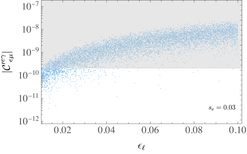
Figure 1: $|\mathcal{C}_{\underset{e\mu}{e\gamma}}^{\prime}|$ in $1/\Lambda^{2}\ [\mathrm{TeV}^{-2}]$ unit versus $\epsilon_{\ell}$, where $s_{e}=0.03$ is put and the grey region is excluded by the experiment of $\mu\to e\gamma$.

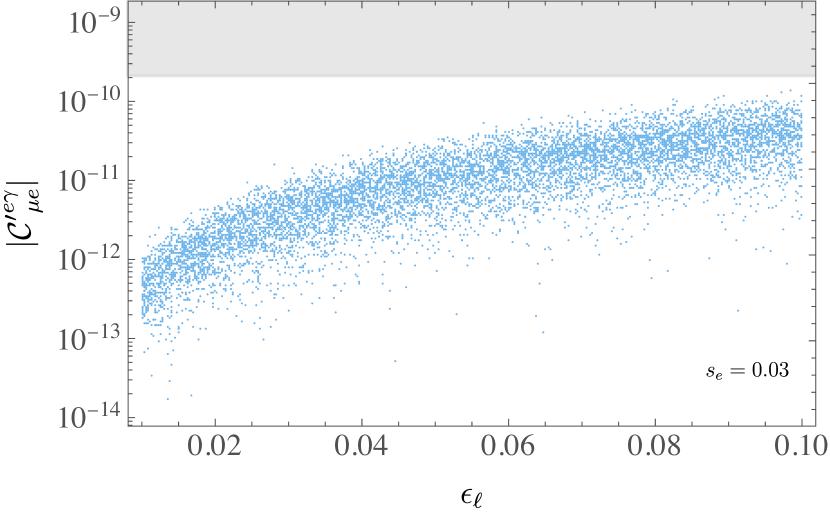
Figure 2: $|\mathcal{C}_{\underset{\mu e}{e\gamma}}^{\prime}|$ in $1/\Lambda^{2}\ [\mathrm{TeV}^{-2}]$ unit versus $\epsilon_{\ell}$, where $s_{e}=0.03$ is put and the grey region is excluded by the experiment of $\mu\to e\gamma$.

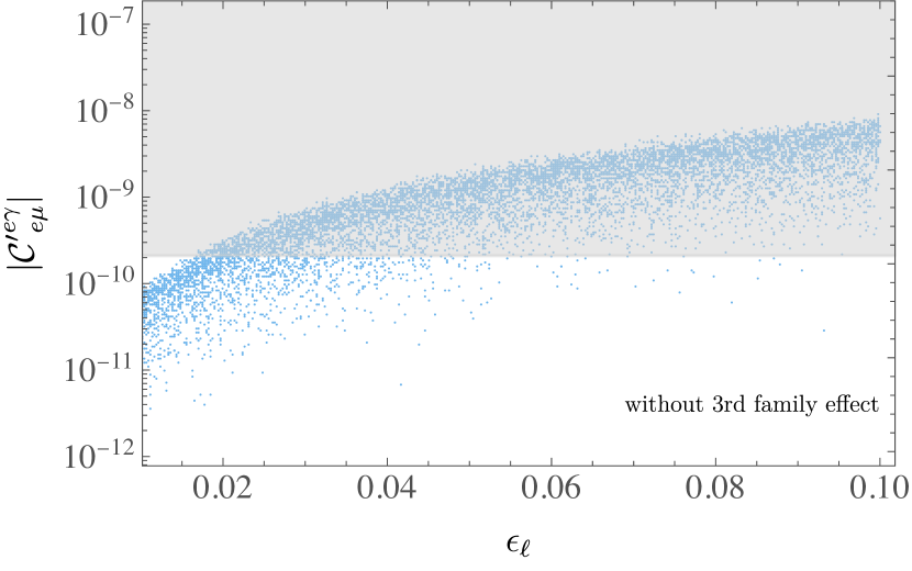
Figure 3: $|\mathcal{C}_{\underset{e\mu}{e\gamma}}^{\prime}|$ in $1/\Lambda^{2}\ [\mathrm{TeV}^{-2}]$ unit versus $\epsilon_{\ell}$ for case (a) (excluding third-family contribution), where $s_{e}=0.03$ is put and the grey region is excluded by the experiment of $\mu\to e\gamma$.

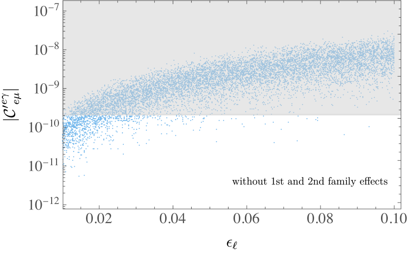
Figure 4: $|\mathcal{C}_{\underset{e\mu}{e\gamma}}^{\prime}|$ in $1/\Lambda^{2}\ [\mathrm{TeV}^{-2}]$ unit versus $\epsilon_{\ell}$ for case (b) (excluding first- and second family contribution ), where $s_{e}=0.03$ is put and the grey region is excluded by the experiment of $\mu\to e\gamma$.

In order to see the contribution of the third-family to $\mathcal{C}_{\underset{e\mu}{e\gamma}}^{\prime}$, we show the magnitude of $\mathcal{C}_{\underset{e\mu}{e\gamma}}^{\prime}$ for both cases of alignment of coefficients (a) $C^{e\gamma}_{V}=C^{y}_{V}$, $C^{e\gamma}_{V\Delta}=C^{y}_{V\Delta}$, $C^{e\gamma}=C^{y}$ and (b) $C^{e\gamma}_{V\Delta}/C^{e\gamma}_{\Delta}=C^{y}_{V\Delta}/C^{y}_{\Delta}$. The case (a) corresponds to the case excluding the third-family contribution and (b) to the case excluding the first- and second-family contribution. The numerical results are presented in Fig. 4 for case (a) and Fig. 4 for case (b). Thus, the third-family contribution is comparable or rather large compared with the one from the first- and second-family.

The $\tau\to\mu\gamma$ decay is an interesting process in $U(2)$ flavor symmetry because it is not suppressed [35]. The upper-bound of the branching ratio of $\tau\to\mu\gamma$ constrains the magnitude of $\epsilon_{\ell}$ as discussed below Eq. (52). We show the magnitude of $\mathcal{C}_{\underset{\mu\tau}{e\gamma}}^{\prime}$ versus $\epsilon_{\ell}$ in Fig. 6, where the predicted value is almost independent of $s_{e}$ as seen in Eq. (51). It is found that small $\epsilon_{\ell}$ (much less than $0.1$) is favored by the experimental upper-bound of the $\tau\to\mu\gamma$ decay. On the other hand, $\mathcal{C}_{\underset{\tau\mu}{e\gamma}}^{\prime}$ is suppressed in more than one order by $\delta_{e}$. We omit a figure for this process.

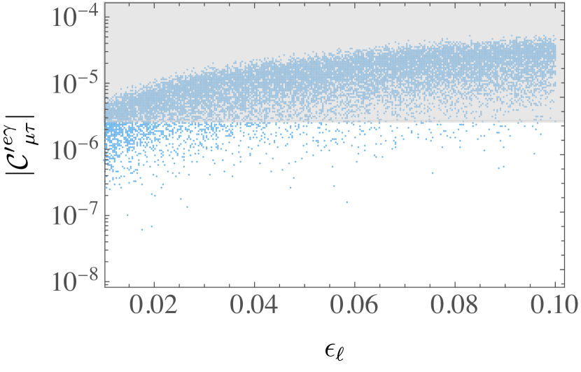
Figure 5: $|\mathcal{C}_{\underset{\mu\tau}{e\gamma}}^{\prime}|$ in $1/\Lambda^{2}\ [\mathrm{TeV}^{-2}]$ unit versus $\epsilon_{\ell}$, where the grey region is excluded by the experiment of $\tau\to\mu\gamma$.

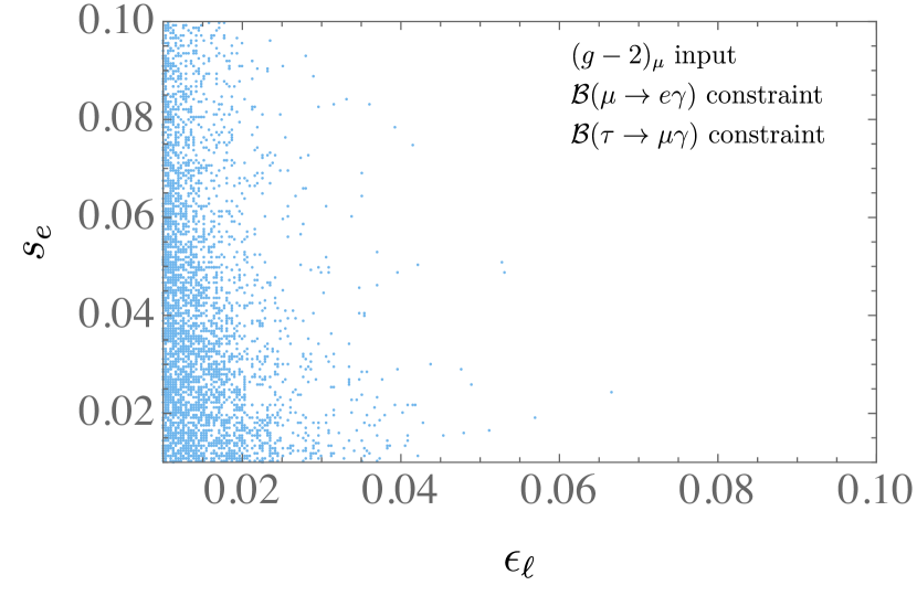
Figure 6: Allowed region in the $\epsilon_{\ell}$-$s_{e}$ plane by the upper-bound of $\mu\to e\gamma$ and $\tau\to\mu\gamma$ branching ratios.

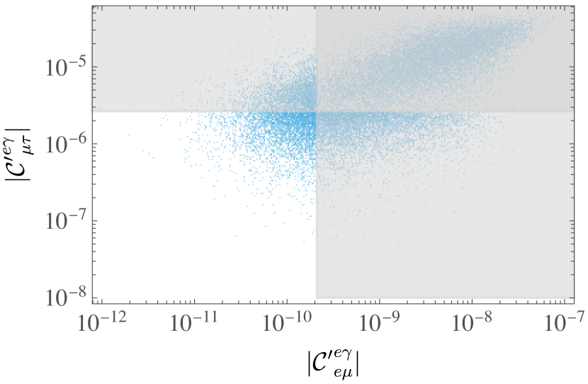
Figure 7: $|\mathcal{C}_{\underset{\mu\tau}{e\gamma}}^{\prime}|$ in $1/\Lambda^{2}\ [\mathrm{TeV}^{-2}]$ unit versus $|\mathcal{C}_{\underset{e\mu}{e\gamma}}^{\prime}|$. The grey region is excluded by the experiments.

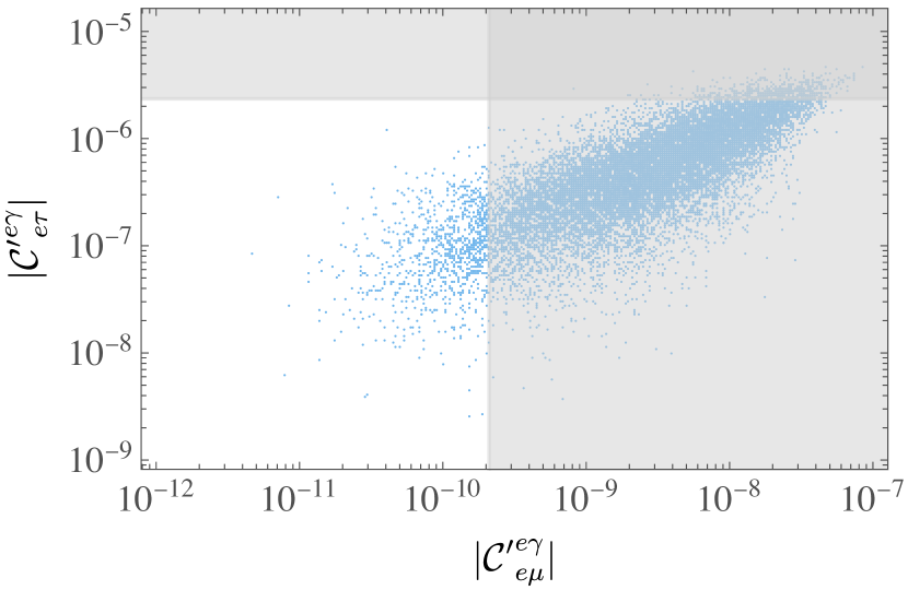
Figure 8: $|\mathcal{C}_{\underset{e\tau}{e\gamma}}^{\prime}|$ in $1/\Lambda^{2}\ [\mathrm{TeV}^{-2}]$ unit versus $|\mathcal{C}_{\underset{e\mu}{e\gamma}}^{\prime}|$. The grey region is excluded by the experiments.

As seen in Figs.2 and 6, the substantial region of predicted Wilson coefficients exceeds the experimental upper-bounds. Imposing the upper-bounds of the branching ratios of $\mu\to e\gamma$ and $\tau\to\mu\gamma$ decays, we obtain the allowed region in $\epsilon_{\ell}$-$s_{e}$ plane in Fig. 6. It is found that $\epsilon_{\ell}$ is almost smaller than $0.05$ while $s_{e}$ is allowed in rather wide range of $[0.01-0.1]$.

In order to see the correlation between $|\mathcal{C}_{\underset{e\mu}{e\gamma}}^{\prime}|$ and $|\mathcal{C}_{\underset{\mu\tau}{e\gamma}}^{\prime}|$, we plot their predictions in Fig. 8. It is found that the allowed region is restricted. In the next subsection, we discuss the expectation value of $\mu\to e\gamma$ and $\tau\to\mu\gamma$.

We also show the predicted region of $|\mathcal{C}_{\underset{e\tau}{e\gamma}}^{\prime}|$ versus $|\mathcal{C}_{\underset{\mu\tau}{e\gamma}}^{\prime}|$ in Fig. 8. The magnitude of $\mathcal{C}_{\underset{e\tau}{e\gamma}}^{\prime}$ is almost proportional to $|\mathcal{C}_{\underset{e\mu}{e\gamma}}^{\prime}|$. The prediction of $\mathcal{C}_{\underset{e\tau}{e\gamma}}^{\prime}$ is still low in one order compared with the experimental upper-bound. It is noted that $\mathcal{C}_{\underset{\tau e}{e\gamma}}^{\prime}$ is suppressed in $\delta^{\prime}_{e}$ as seen in Eq. (42). We omit a figure for this process.

4.3 Predictions of EDM

In the allowed region of $\epsilon_{\ell}$ and $s_{e}$ in Fig. 6, we discuss the EDM of the charged leptons. The electron EDM comes from the imaginary part of $\mathcal{C}_{\underset{ee}{e\gamma}}^{\prime}$. The magnitude is estimated approximately from Eq. (40). This ratio is bounded by the observed constraints in Eqs. (11) and(18) as:

$$\left|\frac{{\rm Im}\ \mathcal{C}_{\underset{ee}{e\gamma}}^{\prime}}{{\rm Re}\ \mathcal{C}_{\underset{\mu\mu}{e\gamma}}^{\prime}}\right|\simeq s_{e}^{2}\frac{\delta^{\prime}}{\delta}\epsilon_{\ell}^{2}\,{\rm Im}\,\left(\frac{C^{e\gamma}_{VV\Delta}}{C^{e\gamma}_{\Delta}}-\frac{C^{y}_{VV\Delta}}{C^{y}_{\Delta}}+\frac{C_{3rd}}{|C^{e\gamma}_{\Delta}|}\right)<1.8\times 10^{-8}\,.$$ (54)

By putting $\epsilon_{\ell}=0.03$ and $s_{e}=0.03$ with $\delta^{\prime}_{e}/\delta_{e}\simeq m_{e}/m_{\mu}$ in Eq. (53), the factor in front of middle side equation, $s_{e}^{2}\epsilon_{\ell}^{2}\delta^{\prime}/\delta$ is $4\times 10^{-9}$. Thus, the ratio is possibly predicted to be ${\cal O}(10^{-8})$, which corresponds to $|d_{e}|\sim 10^{-30}\,{\rm e\,cm}$. We expect it to be detectable in the near future.

We show the plot of ${\rm Im}\ \mathcal{C}_{\underset{ee}{e\gamma}}^{\prime}$ versus $\mathcal{C}_{\underset{e\mu}{e\gamma}}^{\prime}$ in Fig. 10. Since we have a ratio approximately:

$$\frac{{\rm Im}\ \mathcal{C}_{\underset{ee}{e\gamma}}^{\prime}}{|\mathcal{C}_{\underset{e\mu}{e\gamma}}^{\prime}|}\simeq\frac{s_{e}}{c_{e}}\frac{\delta^{\prime}}{\delta}\frac{{\rm Im}\,\left(\frac{C^{e\gamma}_{VV\Delta}}{C^{e\gamma}_{\Delta}}-\frac{C^{y}_{VV\Delta}}{C^{y}_{\Delta}}+\frac{C_{3rd}}{|C^{e\gamma}_{\Delta}|}\right)}{\left|\frac{C^{e\gamma}_{VV\Delta}}{C^{e\gamma}_{\Delta}}-\frac{C^{y}_{VV\Delta}}{C^{y}_{\Delta}}+\frac{C_{3rd}}{|C^{e\gamma}_{\Delta}|}\right|}\,,$$ (55)

we estimate it to be ${\cal O}(10^{-4})$, which is confirmed in Fig. 10. The predicted electron EDM is below the experimental upper-bound after taking account of the upper-bound of $\mathcal{B}({\mu\to e\gamma})$. In the next subsection, we discuss the expectation value of the electron EDM.

We also present the predicted region of EDMs of muon and tauon in Fig. 10. Those are still far from the present experimental upper-bounds, $|{d_{\mu}}|<1.8\times 10^{-19}\,\rm e\,cm$ [21] and $|d_{\tau}|<1.85\times 10^{-17}{\rm e\,cm}$ [24] as seen in Eqs. (4) and (6).

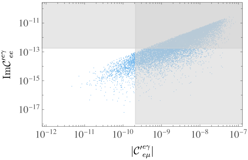
Figure 9: ${\rm Im}\ \mathcal{C}_{\underset{ee}{e\gamma}}^{\prime}$ versus $|\mathcal{C}_{\underset{e\mu}{e\gamma}}^{\prime}|$ (electron EDM versus $\mu\to e\gamma$) in $1/\Lambda^{2}\ [\mathrm{TeV}^{-2}]$ unit. The grey region is excluded by the experiments.

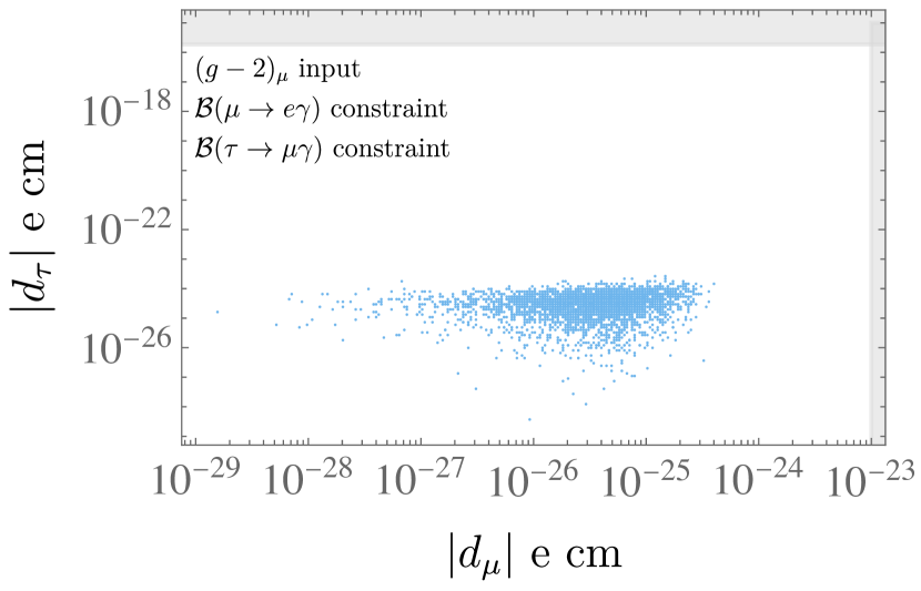
Figure 10: Predicted EDMs of muon and tauon in $[\rm e\,cm]$ unit. The grey region is excluded by the experiments.

4.4 Expectation of $\mu\to e\gamma$, $\tau\to\mu\gamma$, $\tau\to e\gamma$ and electron EDM

Since we have performed the random scan in the linear space of $s_{e}$ and $\epsilon_{\ell}$ in $[0.01-0.1]$ as given in Eq. (30), we can show the frequency distribution of the predicted LFV decays and the electron EDM. Indeed, we obtain the frequency distribution of the predicted $\mathcal{B}({\mu\to e\gamma})$ with imposing contraints of the upper-bound of $\mathcal{B}(\tau\to\mu\gamma)$ and the electron EDM in Fig. 12. The frequency is normalized by total sum being $1$. The grey region is already excluded by the experimental upper-bound of $\mathcal{B}({\mu\to e\gamma})$. The maximal peak is almost inside the grey region. Since the future sensitivity at the MEG II experiment is $\mathcal{B}({\mu\to e\gamma})=6\times 10^{-14}$ [66], we expect the observation of $\mu\to e\gamma$ decay in the near future.

In Fig. 12, we plot the frequency distribution of the predicted $\mathcal{B}({\tau\to\mu\gamma})$ with imposing constraints of the upper-bound of $\mathcal{B}(\mu\to e\gamma)$ and the electron EDM. The peak is also inside the grey region. We also expect the observation of $\tau\to\mu\gamma$ decay in the near future.

In Fig. 14, we plot the frequency distribution of the predicted $\mathcal{B}({\tau\to e\gamma})$ with (without) imposing the upper-bounds of $\mu\to e\gamma$, $\tau\to\mu\gamma$ and the electron EDM with the color of orange (blue). Due to those constraints, the predicted $\mathcal{B}({\tau\to e\gamma})$ is far from the present experimental upper-bound, smaller than three order.

Finally, we plot the frequency distribution of the predicted electron EDM with (without) imposing the upper-bounds of $\mu\to e\gamma$ and $\tau\to\mu\gamma$ with the color of orange (blue) in Fig. 14. Due to those constraints, the peak appears arpond $|d_{e}|\simeq 3\times 10^{-31}$e cm. Since the future sensitivity at ACME $\rm I\hskip-1.13791ptI\hskip-1.13791ptI$ is expected to be $|d_{e}|<3\times 10^{-31}\,\text{e\,cm}$ [19, 20], the electron EDM will be possibly observed in the near future.

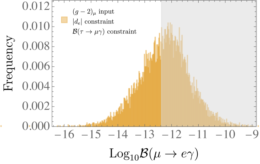
Figure 11: The frequency distribution of the predicted $\mathcal{B}({\mu\to e\gamma})$ with imposing the upper-bounds of $\tau\to\mu\gamma$ decay and the electron EDM. The grey region is excluded by the experimental data of $\mathcal{B}({\mu\to e\gamma})$.

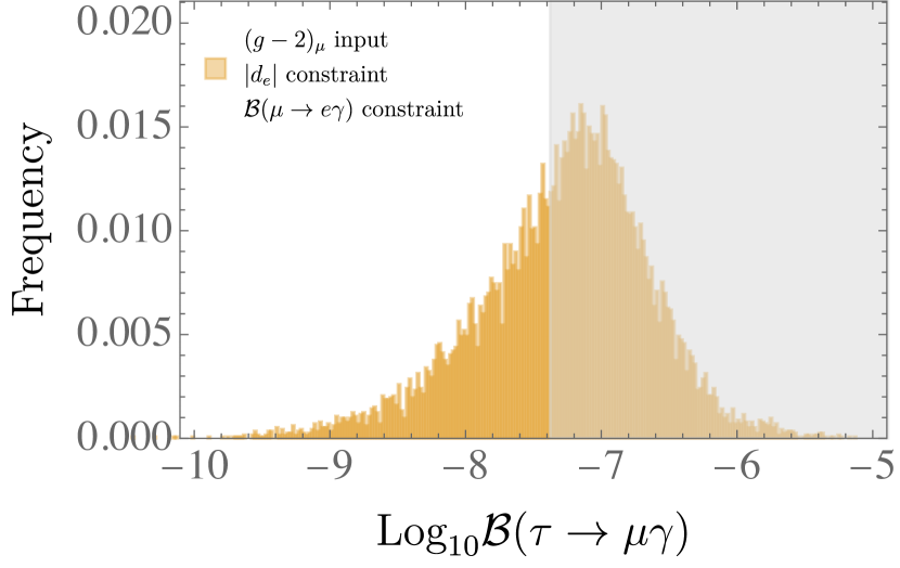
Figure 12: The frequency distribution of the predicted $\mathcal{B}({\tau\to\mu\gamma})$ with imposing the upper-bound of the $\mu\to e\gamma$ decay and the electron EDM. The grey region is excluded by the experimental data of $\mathcal{B}({\tau\to\mu\gamma})$.

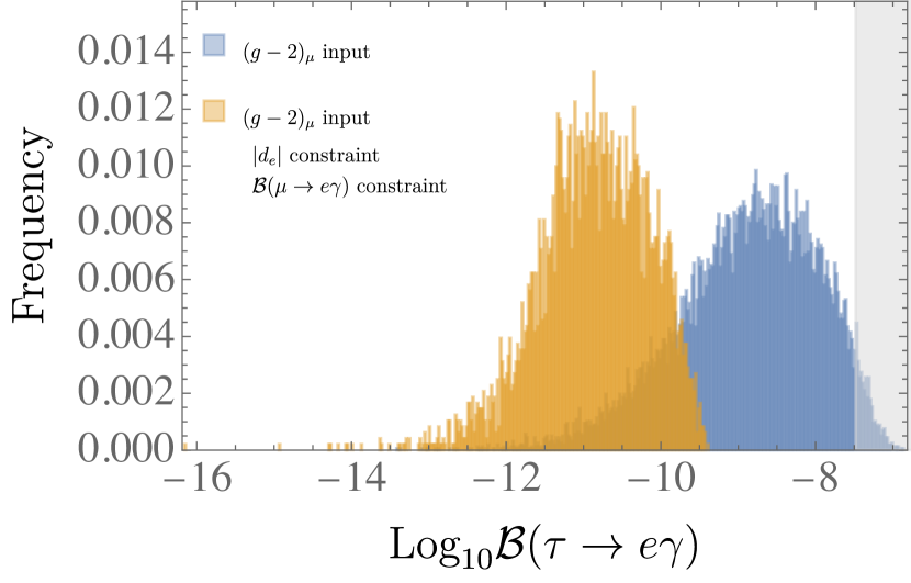
Figure 13: The orange (blue) frequency distribution of the predicted $\mathcal{B}({\tau\to e\gamma})$ with (without) imposing the upper-bounds of the $\mu\to e\gamma$ decay, $\tau\to\mu\gamma$ decay and the electron EDM. The grey region is excluded by the experimental data of $\mathcal{B}({\tau\to e\gamma})$.

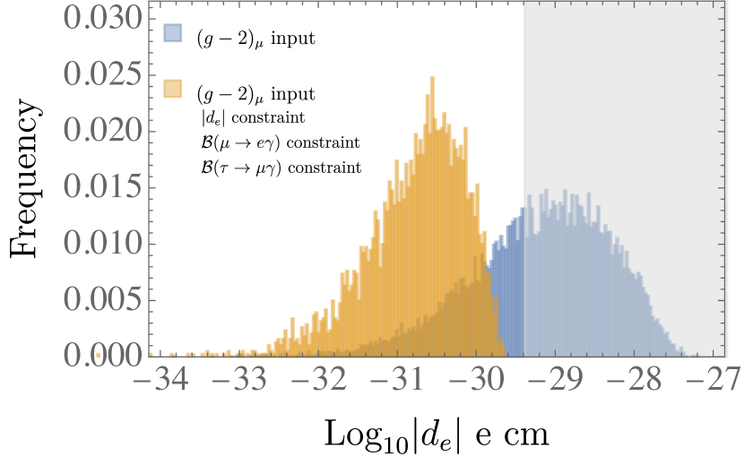
Figure 14: The orange (blue) frequency distribution of the predicted electron EDM $[\rm e\,cm]$ with (without) imposing the $\mu\to e\gamma$ decay and $\tau\to\mu\gamma$ decay. The grey region is excluded by the experimental data of the electron EDM.

5 Summary and discussions

We have studied the interplay of NP among the lepton magnetic moments, LFV and the electron EDM in the light of recent data of the muon $(g-2)_{\mu}$. The NP is discussed in the leptonic dipole operator with the $U(2)_{L_{L}}\otimes U(2)_{E_{R}}$ flavor symmetry of the charged leptons, where possible CP violating phases of the three family space are taken into account. It is remarked that the the third-family contributes significantly to the $\mu\to e\gamma$ decay and the electron EDM. Indeed, the $\mu\to e\gamma$ process is not suppressed even if the contribution of the first- and second-family vanishes. The electron EDM is also predicted to be rather large due to the CP violating phase in the third-family even if the CP phase of the first- and second-family is zero.

In addition, we have also discussed the electron and tauon $(g-2)_{e,\tau}$ and the EDM of the muon and tauon as well as LFV processes $\tau\to\mu\gamma$ and $\tau\to e\gamma$. In particular, the $\tau_{R}\to\mu_{L}\gamma$ process is predicted close to the experimental upper-bound due to the $\mu_{L}$-$\tau_{L}$ mixing of ${\cal O}(\epsilon_{\ell})$. This decay will be possibly observed in the near future in Belle II experiment [64, 65]. The $\tau_{R}\to e_{L}\gamma$ decay is not suppressed due to the $e_{L}$-$\mu_{L}$ mixing of ${\cal O}(s_{e})$ together with the $\mu_{L}$-$\tau_{L}$ mixing. On the other hand, the $\mu_{L}\to e_{R}\gamma$, $\tau_{L}\to\mu_{R}\gamma$ and $\tau_{L}\to e_{R}\gamma$ decays are suppressed. The angular distribution with respect to the muon polarization can distinguish between $\mu_{R}\to e_{L}\gamma$ and $\mu_{L}\to e_{R}\gamma$.

The expected values of LFV decays and the electron EDM are presented in the frequency distribution of them. The electron EDM will be possibly observed as well as the $\mu\to e\gamma$ and $\tau\to\mu\gamma$ decays in the near future.

In our numerical analyses, we have put $\Delta a_{\mu}=249\times 10^{-11}$ for the NP effect. If $\Delta a_{\mu}$ is significantly lower, less than or of order $1\,\sigma$, we obtain somewhat different prediction for the interplay among the muon $(g-2)_{\mu}$, the electron EDM and the $\mu\to e\gamma$ decay. For example, if we take the input $\Delta a_{\mu}\simeq 50\times 10^{-11}$, which is of order $1\,\sigma$. Our predicted LFV branching ratios are reduced by $1/25$ while predictions of $(g-2)_{e,\tau}$ and EDM’s are reduced by $1/5$. We need the precise value of the SM prediction of HVP to make our numerical result of NP contributions to LFV and EDM reliable.

Acknowledgement
This work was supported by JSPS KAKENHI Grant Number JP21K13923 (KY).

Appendix

Appendix A Experimental constraints on the dipole operators

From the experimental data of the muon $(g-2)_{\mu}$ and ${\mu\to e\gamma}$, Ref. [35] gave the constraints on the dipole operators. We summarize briefly them on the dipole operators in Eq. (9). Below the scale of electroweak symmetry breaking, the leptonic dipole operators are given as:

$$\mathcal{O}_{\underset{rs}{e\gamma}}=\frac{v}{\sqrt{2}}\overline{e}_{L_{r}}\sigma^{\mu\nu}e_{R_{s}}F_{\mu\nu}\,,$$ (56)

where $\{r,s\}$ are flavor indices $e,\mu,\tau$ and $F_{\mu\nu}$ is the electromagnetic field strength tensor. The effective Lagrangian is

$$\mathcal{L}_{\rm dipole}=\frac{1}{\Lambda^{2}}\,\left(\mathcal{C}_{\underset{rs}{e\gamma}}^{\prime}\mathcal{O}_{\underset{rs}{e\gamma}}+\mathcal{C}_{\underset{es}{e\gamma}}^{\prime}\mathcal{O}_{\underset{rs}{e\gamma}}\right)\,,$$ (57)

where $\Lambda$ is a certain mass scale of NP in the effective theory. The corresponding Wilson coefficient $\mathcal{C}_{\underset{rs}{e\gamma}}^{\prime}$ is denoted in the mass-eigenstate basis of leptons.

The tree-level expression for $\Delta a_{\mu}$ in terms of the Wilson coefficient of the dipole operator is

$$\Delta a_{\mu} =\frac{4m_{\mu}}{e}\frac{v}{\sqrt{2}}\,\frac{1}{\Lambda^{2}}\text{Re}\,[\mathcal{C}_{\underset{\mu\mu}{e\gamma}}^{\prime}]\,,$$ (58)

where $v\approx 246$ GeV. Let us input the value

$$\Delta a_{\mu}=249\times 10^{-11}~{}\,,$$ (59)

then, we obtain the Willson coefficient as:

$$\frac{1}{\Lambda^{2}}\text{Re}\ [\mathcal{C}_{\underset{\mu\mu}{e\gamma}}^{\prime}]=1.0\times 10^{-5}\,\mathrm{TeV}^{-2}\,,$$ (60)

where $e\simeq 0.3028$ is put in the natural unit.

The tree-level expression of a radiative LFV rate in terms of the Wilson coefficients is

$$\mathcal{B}(\ell_{r}\to\ell_{s}\gamma)=\frac{m_{\ell_{r}}^{3}v^{2}}{8\pi\Gamma_{\ell_{r}}}\frac{1}{\Lambda^{4}}\left(|\mathcal{C}_{\underset{rs}{e\gamma}}^{\prime}|^{2}+|\mathcal{C}_{\underset{sr}{e\gamma}}^{\prime}|^{2}\right)\,.$$ (61)

Taking the experimental bound $\mathcal{B}\!\left(\mu^{+}\to e^{+}\gamma\right)<4.2\times 10^{-13}$ (90% C.L.) obtained by the MEG experiment [25] in Eq. (7), we obtain the upper-bound of the Wilson coefficient as:

$$\frac{1}{\Lambda^{2}}|\mathcal{C}_{\underset{e\mu(\mu e)}{e\gamma}}^{\prime}|<2.1\times 10^{-10}\,\mathrm{TeV}^{-2}\,.$$ (62)

On the other hand, by taking the following experimental upper-bound of the branching ratios, $\mathcal{B}\!\left(\tau\to\mu+\gamma\right)<4.2\times 10^{-8}$ and $\mathcal{B}\!\left(\tau\to e\gamma\right)<3.3\times 10^{-8}$ [26, 27], we obtain the upper-bound of the Wilson coefficient as:

$$\frac{1}{\Lambda^{2}}|\mathcal{C}_{\underset{\mu\tau(\tau\mu)}{e\gamma}}^{\prime}|<2.65\times 10^{-6}\,\mathrm{TeV}^{-2}\,,\qquad\frac{1}{\Lambda^{2}}|\mathcal{C}_{\underset{e\tau(\tau e)}{e\gamma}}^{\prime}|<2.35\times 10^{-6}\,\mathrm{TeV}^{-2}\,,$$ (63)

respectively.

Appendix B Explicit forms of $3\times 3$ matrices for $YY^{\dagger}$ and $Y^{\dagger}Y$

Here, we present the $3\times 3$ matrices for $YY^{\dagger}$ and $Y^{\dagger}Y$ by using Eq. (24) explicitly. We can obtain the left (right)-handed mixing angles and phases by using these Hermitian matrices. The left-handed mixing is obtained by diagonalizing $YY^{\dagger}$, which is:

$$YY^{\dagger}=$$

$$\begin{pmatrix}{C^{y}_{\Delta}}^{2}(c_{e}^{2}{\delta^{\prime}_{e}}^{2}+s_{e}^{2}\delta_{e}^{2})&C^{y}_{\Delta}(C^{y\,*}_{\Delta}+C^{y\,*}_{VV\Delta}\epsilon^{2}_{\ell})({\delta^{\prime}_{e}}^{2}-{\delta_{e}}^{2})c_{e}s_{e}&[3,1]^{*}\\ [1.2]^{*}&|(C^{y}_{\Delta}+C^{y}_{VV\Delta}\epsilon^{2}_{\ell})|^{2}(s_{e}^{2}{\delta^{\prime}_{e}}^{2}+c_{e}^{2}\delta_{e}^{2})+|C^{y}_{V}|^{2}\epsilon^{2}_{\ell}&[3,2]^{*}\\ C^{y\,*}_{\Delta}C^{y}_{V\Delta}({\delta^{\prime}_{e}}^{2}-{\delta_{e}}^{2})c_{e}s_{e}\epsilon_{\ell}&[C^{y\,*}_{V\Delta}(C^{y\,*}_{\Delta}+C^{y\,*}_{VV\Delta}\epsilon^{2}_{\ell})(s_{e}^{2}{\delta^{\prime}_{e}}^{2}+c_{e}^{2}\delta_{e}^{2})+C^{y\,*}_{V}C^{y}]\,\epsilon_{\ell}&|C^{y}|^{2}+(s_{e}^{2}{\delta^{\prime}_{e}}^{2}+c_{e}^{2}\delta_{e}^{2})|C^{y}_{V\Delta}|^{2}\end{pmatrix}.$$ (64)

On the other hand, the right-handed mixing is obtained by diagonalizing $Y^{\dagger}Y$, which is:

$$Y^{\dagger}Y=$$

$$\begin{pmatrix}[{C^{y}_{\Delta}}^{2}c_{e}^{2}+(|C^{y}_{\Delta}+C^{y}_{VV\Delta}\epsilon^{2}_{\ell}|^{2}+|C^{y}_{V\Delta}|^{2}\epsilon^{2}_{\ell})s_{e}^{2}]{\delta^{\prime}_{e}}^{2}&(2{\rm Re}{C^{y}_{\Delta}}+|C^{y}_{VV\Delta}|^{2}\epsilon^{2}_{\ell}+|C^{y}_{V\Delta}|^{2})\delta^{\prime}_{e}\delta_{e}\epsilon^{2}_{\ell}c_{e}s_{e}&[3,1]^{*}\\ [1,2]^{*}&[{C^{y}_{\Delta}}^{2}s_{e}^{2}+(|C^{y}_{\Delta}+C^{y}_{VV\Delta}\epsilon^{2}_{\ell}|^{2}+|C^{y}_{V\Delta}|^{2}\epsilon^{2}_{\ell})c_{e}^{2}]{\delta_{e}}^{2}&[3,2]^{*}\\ (C^{y}_{\Delta}C^{y\,*}_{V}+C^{y}_{V}C^{y\,*}+C^{y}_{VV\Delta}C^{y\,*}_{V}\epsilon^{2}_{\ell})\delta^{\prime}_{e}\epsilon_{\ell}s_{e}&(C^{y}_{\Delta}C^{y\,*}_{V}+C^{y}_{V\Delta}C^{y\,*}+C^{y}_{VV\Delta}C^{y\,*}_{V}\epsilon^{2}_{\ell})\delta_{e}\epsilon_{\ell}c_{e}&|C^{y}|^{2}+|C^{y}_{V}|^{2}\epsilon^{2}_{\ell}\end{pmatrix}.$$ (65)

References

- [1] D. P. Aguillard et al. [Muon g-2], [arXiv:2308.06230 [hep-ex]].
- [2] B. Abi et al. [Muon g-2], Phys. Rev. Lett. 126 (2021) no.14, 141801 [arXiv:2104.03281 [hep-ex]].
- [3] G. W. Bennett et al. [Muon g-2], Phys. Rev. D 73 (2006), 072003 [arXiv:hep-ex/0602035 [hep-ex]].
- [4] T. Aoyama, N. Asmussen, M. Benayoun, J. Bijnens, T. Blum, M. Bruno, I. Caprini, C. M. Carloni Calame, M. Cè and G. Colangelo, et al. Phys. Rept. 887 (2020), 1-166 [arXiv:2006.04822 [hep-ph]].
- [5] F. Jegerlehner, Springer Tracts Mod. Phys. 274 (2017), pp.1-693.
- [6] G. Colangelo, M. Hoferichter and P. Stoffer, JHEP 02 (2019), 006 [arXiv:1810.00007 [hep-ph]].
- [7] M. Hoferichter, B. L. Hoid and B. Kubis, JHEP 08 (2019), 137 [arXiv:1907.01556 [hep-ph]].
- [8] M. Davier, A. Hoecker, B. Malaescu and Z. Zhang, Eur. Phys. J. C 80 (2020) no.3, 241 [erratum: Eur. Phys. J. C 80 (2020) no.5, 410] [arXiv:1908.00921 [hep-ph]].
- [9] A. Keshavarzi, D. Nomura and T. Teubner, Phys. Rev. D 101 (2020) no.1, 014029 [arXiv:1911.00367 [hep-ph]].
- [10] B. L. Hoid, M. Hoferichter and B. Kubis, Eur. Phys. J. C 80 (2020) no.10, 988 [arXiv:2007.12696 [hep-ph]].
- [11] A. Czarnecki, W. J. Marciano and A. Vainshtein, Phys. Rev. D 67 (2003), 073006 [erratum: Phys. Rev. D 73 (2006), 119901] [arXiv:hep-ph/0212229 [hep-ph]].
- [12] K. Melnikov and A. Vainshtein, Phys. Rev. D 70 (2004), 113006 [arXiv:hep-ph/0312226 [hep-ph]].
- [13] T. Aoyama, M. Hayakawa, T. Kinoshita and M. Nio, Phys. Rev. Lett. 109 (2012), 111808 [arXiv:1205.5370 [hep-ph]].
- [14] C. Gnendiger, D. Stöckinger and H. Stöckinger-Kim, Phys. Rev. D 88 (2013), 053005 [arXiv:1306.5546 [hep-ph]].
- [15] F. V. Ignatov et al. [CMD-3], [arXiv:2302.08834 [hep-ex]].
- [16] S. Borsanyi, Z. Fodor, J. N. Guenther, C. Hoelbling, S. D. Katz, L. Lellouch, T. Lippert, K. Miura, L. Parato and K. K. Szabo, et al. Nature 593 (2021) no.7857, 51-55 [arXiv:2002.12347 [hep-lat]].
- [17] T. S. Roussy, L. Caldwell, T. Wright, W. B. Cairncross, Y. Shagam, K. B. Ng, N. Schlossberger, S. Y. Park, A. Wang and J. Ye, et al. Science 381 (2023) no.6653, adg4084 [arXiv:2212.11841 [physics.atom-ph]].
- [18] V. Andreev et al. [ACME], Nature 562 (2018) no.7727, 355-360.
- [19] D. M. Kara, I. J. Smallman, J. J. Hudson, B. E. Sauer, M. R. Tarbutt and E. A. Hinds, New J. Phys. 14 (2012), 103051 [arXiv:1208.4507 [physics.atom-ph]].
- [20] J. Doyle, “Search for the Electric Dipole Moment of the Electron with Thorium Monoxide - The ACME Experiment.”Talk at the KITP, September 2016.
- [21] G. W. Bennett et al. [Muon (g-2)], Phys. Rev. D 80 (2009), 052008 [arXiv:0811.1207 [hep-ex]].
- [22] K. Inami et al. [Belle], Phys. Lett. B 551 (2003), 16-26 [arXiv:hep-ex/0210066 [hep-ex]].
- [23] W. Bernreuther, L. Chen and O. Nachtmann, Phys. Rev. D 103 (2021) no.9, 096011 [arXiv:2101.08071 [hep-ph]].
- [24] K. Uno, PoS ICHEP2022 (2022), 721.
- [25] A. M. Baldini et al. [MEG], Eur. Phys. J. C 76 (2016) no.8, 434 [arXiv:1605.05081 [hep-ex]].
- [26] B. Aubert et al. [BaBar], Phys. Rev. Lett. 104 (2010), 021802 [arXiv:0908.2381 [hep-ex]].
- [27] A. Abdesselam et al. [Belle], JHEP 10 (2021), 19 [arXiv:2103.12994 [hep-ex]].
- [28] W. Buchmuller and D. Wyler, Nucl. Phys. B 268 (1986), 621-653.
- [29] B. Grzadkowski, M. Iskrzynski, M. Misiak and J. Rosiek, JHEP 10 (2010), 085 [arXiv:1008.4884 [hep-ph]].
- [30] R. Alonso, E. E. Jenkins, A. V. Manohar and M. Trott, JHEP 04 (2014), 159 [arXiv:1312.2014 [hep-ph]].
- [31] G. Panico, A. Pomarol and M. Riembau, JHEP 04 (2019), 090 [arXiv:1810.09413 [hep-ph]].
- [32] J. Aebischer, W. Dekens, E. E. Jenkins, A. V. Manohar, D. Sengupta and P. Stoffer, JHEP 07 (2021), 107 [arXiv:2102.08954 [hep-ph]].
- [33] L. Allwicher, P. Arnan, D. Barducci and M. Nardecchia, JHEP 10 (2021), 129 [arXiv:2108.00013 [hep-ph]].
- [34] J. Kley, T. Theil, E. Venturini and A. Weiler, [arXiv:2109.15085 [hep-ph]].
- [35] G. Isidori, J. Pagès and F. Wilsch, JHEP 03 (2022), 011 [arXiv:2111.13724 [hep-ph]].
- [36] R. Barbieri, G. Isidori, J. Jones-Perez, P. Lodone and D. M. Straub, Eur. Phys. J. C 71 (2011), 1725 [arXiv:1105.2296 [hep-ph]].
- [37] R. Barbieri, D. Buttazzo, F. Sala and D. M. Straub, JHEP 07 (2012), 181 [arXiv:1203.4218 [hep-ph]].
- [38] G. Blankenburg, G. Isidori and J. Jones-Perez, Eur. Phys. J. C 72 (2012), 2126 [arXiv:1204.0688 [hep-ph]].
- [39] J. Fuentes-Martín, G. Isidori, J. Pagès and K. Yamamoto, Phys. Lett. B 800 (2020), 135080 [arXiv:1909.02519 [hep-ph]].
- [40] D. A. Faroughy, G. Isidori, F. Wilsch and K. Yamamoto, JHEP 08 (2020), 166 [arXiv:2005.05366 [hep-ph]].
- [41] T. Kobayashi, H. Otsuka, M. Tanimoto and K. Yamamoto, Phys. Rev. D 105 (2022) no.5, 055022 [arXiv:2112.00493 [hep-ph]].
- [42] T. Kobayashi, H. Otsuka, M. Tanimoto and K. Yamamoto, JHEP 08 (2022), 013 [arXiv:2204.12325 [hep-ph]].
- [43] T. Kobayashi and H. Otsuka, Eur. Phys. J. C 82 (2022) no.1, 25 [arXiv:2108.02700 [hep-ph]].
- [44] L. Calibbi, M. L. López-Ibáñez, A. Melis and O. Vives, Eur. Phys. J. C 81 (2021) no.10, 929 [arXiv:2104.03296 [hep-ph]].
- [45] G. Altarelli and F. Feruglio, Rev. Mod. Phys. 82 (2010) 2701 [arXiv:1002.0211 [hep-ph]].
- [46] H. Ishimori, T. Kobayashi, H. Ohki, Y. Shimizu, H. Okada and M. Tanimoto, Prog. Theor. Phys. Suppl. 183 (2010) 1 [arXiv:1003.3552 [hep-th]].
- [47] H. Ishimori, T. Kobayashi, H. Ohki, H. Okada, Y. Shimizu and M. Tanimoto, Lect. Notes Phys. 858 (2012) 1, Springer.
- [48] T. Kobayashi, H. Ohki, H. Okada, Y. Shimizu and M. Tanimoto, Lect. Notes Phys. 995 (2022) 1, Springer doi:10.1007/978-3-662-64679-3.
- [49] D. Hernandez and A. Y. Smirnov, Phys. Rev. D 86 (2012) 053014 [arXiv:1204.0445 [hep-ph]].
- [50] S. F. King and C. Luhn, Rept. Prog. Phys. 76 (2013) 056201 [arXiv:1301.1340 [hep-ph]].
- [51] S. F. King, A. Merle, S. Morisi, Y. Shimizu and M. Tanimoto, New J. Phys. 16, 045018 (2014) [arXiv:1402.4271 [hep-ph]].
- [52] M. Tanimoto, AIP Conf. Proc. 1666 (2015) 120002.
- [53] S. F. King, Prog. Part. Nucl. Phys. 94 (2017) 217 [arXiv:1701.04413 [hep-ph]].
- [54] S. T. Petcov, Eur. Phys. J. C 78 (2018) no.9, 709 [arXiv:1711.10806 [hep-ph]].
- [55] F. Feruglio and A. Romanino, Rev. Mod. Phys. 93 (2021) no.1, 015007 [arXiv:1912.06028 [hep-ph]].
- [56] Q. Shafi, A. Tiwari and C. S. Un, [arXiv:2308.14682 [hep-ph]].
- [57] D. Buttazzo and P. Paradisi, Phys. Rev. D 104 (2021) no.7, 075021 [arXiv:2012.02769 [hep-ph]].
- [58] G. F. Giudice, P. Paradisi and M. Passera, JHEP 11 (2012), 113 [arXiv:1208.6583 [hep-ph]].
- [59] D. Hanneke, S. Fogwell and G. Gabrielse, Phys. Rev. Lett. 100 (2008), 120801 [arXiv:0801.1134 [physics.atom-ph]].
- [60] R. H. Parker, C. Yu, W. Zhong, B. Estey and H. Müller, Science 360 (2018), 191 [arXiv:1812.04130 [physics.atom-ph]].
- [61] L. Morel, Z. Yao, P. Cladé, and S. Guellati-Khélifa, Nature 588 (2020), no.7836 61-65.
- [62] S. Nishimura, C. Miyao and H. Otsuka, [arXiv:2304.14176 [hep-ph]].
- [63] Y. Okada, K. i. Okumura and Y. Shimizu, Phys. Rev. D 61 (2000), 094001 [arXiv:hep-ph/9906446 [hep-ph]].
- [64] E. Kou et al. [Belle-II], PTEP 2019 (2019) no.12, 123C01 [erratum: PTEP 2020 (2020) no.2, 029201] [arXiv:1808.10567 [hep-ex]].
- [65] A. De Yta Hernández [Belle II], PoS EPS-HEP2021 (2022), 527.
- [66] A. M. Baldini et al. [MEG II], Eur. Phys. J. C 78 (2018) no.5, 380 [arXiv:1801.04688 [physics.ins-det]].