The physical origin of the periodic activity for FRB 20180916B

Abstract

Fast radio bursts (FRBs) are transient radio signals with millisecond-duration, large dispersion measure (DM) and extremely high brightness temperature. Among them, FRB 20180916B has been found to have a 16-day periodic activity. However, the physical origin of the periodicity is still a mystery. Here, we utilize the comprehensive observational data to diagnose the periodic models. We find that the ultra-long rotation model is the most probable one for the periodic activity. However, this model cannot reproduce the observed rotation measure (RM) variations. We propose a self-consistent model, i.e., a massive binary containing a slowly rotational neutron star and a massive star with large mass loss, which can naturally accommodate the wealth of observational features for FRB 20180916B. In this model, the RM variation is periodic, which can be tested by future observations.

1 Introduction

Fast radio bursts (FRBs) are transient radio signals which have a milliseconds-duration, large DM and extremely high brightness temperature (Cordes & Chatterjee, 2019; Xiao et al., 2021; Zhang, 2023). They were first discovered in 2007 and then were verified in 2013 (Lorimer et al., 2007; Thornton et al., 2013). Since then, hundreds of FRB sources had been detected and they are classified as repeating FRBs and non-repeating FRBs. Among the repeating FRBs, FRB 20180916B (Chime/Frb Collaboration et al., 2020) and FRB 20121102 (Rajwade et al., 2020; Cruces et al., 2021) are found to have a period of 16.35d and 157 d, which offers a great opportunity to study the physical origin of FRBs. FRB 20180916B is a repeating FRB source first detected by the Canadian Hydrogen Intensity Mapping Experiment (CHIME) (CHIME/FRB Collaboration et al., 2019) and it was localized to a star-forming region in a nearby massive spiral galaxy with a redshift of $0.0337$ (Marcote et al., 2020). Different from many other FRB sources, FRB 20180916B exhibits a period of 16.35 days and an active window of five days (Chime/Frb Collaboration et al., 2020). With the help of the follow-up observational data from the Low-Frequency Array (LOFAR) (Pastor-Marazuela et al., 2021; Pleunis et al., 2021a) and Apertif (Pastor-Marazuela et al., 2021), the active window shows a strong dependency on frequency, with higher frequency having a narrower active window and the phase center of higher frequency occurring earlier than the lower frequency (Pastor-Marazuela et al., 2021). For other observational properties, the DM of FRB 20180916B is approximately $349$ pc cm^-3 and its variation between different bursts is very small ($\Delta$DM $<1$ pc cm^-3) (CHIME/FRB Collaboration et al., 2019; Mckinven et al., 2023; Pastor-Marazuela et al., 2021). The RM of FRB 20180916B keeps stable (Mckinven et al., 2023) in the first three years after its discovery in 2018. Then the RM increases monotonically over a 9 month duration to $-54.4$ rad m^-2. But the RM variations is unrelated to the 16.3-day period (Mckinven et al., 2023). For a single burst, the variation of linear polarization angle is less than $10^{\circ}\sim 20^{\circ}$ and for different bursts, the variation of linear polarization angle is less than $50^{\circ}$ (Nimmo et al., 2021; Pleunis et al., 2021a).

To explain this special periodic activity, numerous models have been proposed. Encouraged by the observation of FRB 20200428 which is associated with SGR J1935+2154 in the Milky Way (CHIME/FRB Collaboration et al., 2020; Bochenek et al., 2020), some theoretical models propose strongly magnetized neutron stars as the emitting source of FRBs. For these models, the periodic activity can be explained by the orbital motion of a binary system with a neutron star and a massive star with mass loss (Lyutikov et al., 2020; Ioka & Zhang, 2020; Wada et al., 2021; Li et al., 2021), the free or forced precession of a neutron star (Levin et al., 2020; Zanazzi & Lai, 2020; Yang & Zou, 2020; Tong et al., 2020) or a ultra-long rotation of a neutron star (Beniamini et al., 2020). A binary system undergoing super-Eddington accretion can also be considered as the source of this FRB and the periodicity can be explained by the precession of the compact star (Katz, 2020; Sridhar et al., 2021). These theoretical models not only make different predictions on the temporal evolution of the observed period (Katz, 2021; Wei et al., 2022), but also on the distribution of various observational parameters, such as DM, polarization angle and RM. There are also some other models, such as a magnetized pulsar traveling through an asteroid belts in a binary system (Dai & Zhong, 2020), a binary system with a neutron star and a white dwarf undergoing mass transfer (Gu et al., 2020), a planet partially disrupted by a neutron star at periastron (Kurban et al., 2022) and a massive binary consisting of a magnetar and an early-type star (Barkov & Popov, 2022). Since they are lack of explicit predictions, we will not discuss them in this work.

The paper is organized as follows. We calculate the period and period derivation of FRB 20180916B in Section 2. Then, we use the observational data to constrain the periodic model in Section 3. Finally, conclusions are given in Section 4.

2 Period and period derivation

Based on the discovery of periodic activity (Chime/Frb Collaboration et al., 2020), the observational data of FRB 20180916B have significantly expanded which offers an opportunity to get a more precise period and its temporal evolution. Firstly, we calculate the period of FRB 20180916B with the epoch-folding method, which had been used to discover its period by CHIME team (Chime/Frb Collaboration et al., 2020). In this method, we first fold the arrival time of each burst into a normalization phase using the following equation

$$\phi=\frac{t-t_{0}}{P}.$$ (1)

where $t_{0}$ is set as MJD $=58369.40$, $\phi$ is the normalization phase and P is the observational period. Then, the Pearson $\chi^{2}$ test is performed on the phase of the bursts against rectangular distribution for a given period. The higher $\chi^{2}$ of the period, the more reliability of the period.

We list the results in Table 1. In the first line of Table 1, we use the 111 bursts detected by CHIME till the middle of 2023 to calculate the period (https://www.chime-frb.ca/). The result is $16.33\pm 0.05$ days, which is similar to the one found by CHIME/FRB (Chime/Frb Collaboration et al., 2020). We also utilize 29 bursts provided by LOFAR (Pastor-Marazuela et al., 2021; Pleunis et al., 2021a; Gopinath et al., 2023) and get a period of $16.32\pm 0.06$ days, which is consistent with the result derived from the data of CHIME, as shown in the second line of Table 1. To investigate the possible temporal evolution of the period, we divide the bursts observed by CHIME into different time bins to calculate the period. In the last five lines of Table 1, we first divide the bursts of CHIME into two time bins. We get $16.33\pm 0.11$ days and $16.32\pm 0.09$ days which are almost the same. Then we divide the bursts of CHIME into three time bins. The results are $16.34\pm 0.17$ days, $16.38\pm 0.17$ days and $16.32\pm 0.11$ days, respectively. These results support that the period of FRB 20180916B possesses a minimal variation, which falls well within the range of the error bar.

Table 1: The period of FRB 20180916B derived from the epoch-folding method.

Telescope	Burst number	Time range	Period (d)	Error (d)	References
CHIME	111	2018.09.16-2023.06.30	16.33	0.05	https://www.chime-frb.ca/
LOFAR	29	2019.08.13-2022.09.28	16.32	0.06	(Pleunis et al., 2021a; Gopinath et al., 2023)
CHIME	56	2018.09.16-2020.11.23	16.33	0.11	(Chime/Frb Collaboration et al., 2020)
CHIME	55	2021-01-11-2023.06.30	16.32	0.09	(Mckinven et al., 2023)
CHIME	37	2018.09.16-2020.02.04	16.34	0.17	(Chime/Frb Collaboration et al., 2020)
CHIME	37	2020.02.04-2021.06.26	16.38	0.17	(Mckinven et al., 2023)
CHIME	37	2021.07.11-2023.06.30	16.32	0.11	https://www.chime-frb.ca/

In order to get a more accurate constraint on the period derivative ($\dot{P}$), we consider the effect of the $\dot{P}$ when calculating the phase in the epoch-folding method, i.e.,

$$\phi=\frac{2\pi(t-t_{0})}{P}-\pi\frac{\dot{P}}{P^{2}}(t-t_{0})^{2},$$ (2)

Two methods are used to estimate $P$ and $\dot{P}$. For the First method, we utilize the epoch-folding method as shown in Equation (2). The two-dimensional Gaussian functions are used to fit the result. The 1$\sigma$ range is taken as the error bar (Sand et al., 2023). We find $P=16.31\pm 0.32$ days and $\dot{P}=-2.4\times 10^{-5}\pm 1.1\times 10^{-4}$ day day^-1, which is consistent with the derivative $\dot{P}=0$. A similar result $\dot{P}=-2.0\times 10^{-5}\pm 1.5\times 10^{-4}$ is also found by CHIME team (Sand et al., 2023). However, it may be not appropriate to assume that the $\chi^{2}$ distributions of $P$ and $\dot{P}$ obeys two-dimensional Gaussian function. So we use the second method to give a $\dot{P}$ ranges for different periods.

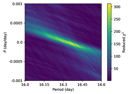
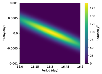
Figure 1: The reduced $\chi^{2}$ of different $P$ and $\dot{P}$. Top panel shows the result of epoch-folding method for different $P$ and $\dot{P}$ with the use of Equation (2). A higher $\chi^{2}$ means that the period and its $\dot{P}$ are more reliable respectively. Bottom panel is the two dimensional Gaussian fitting results of the top panel.

For the second method, we use the earlier 56 bursts from CHIME to establish an active window, and then verify if the subsequent 55 bursts fall within the active window. This method is similar to the one used to get the error bar of the period of FRB 20180916B (Chime/Frb Collaboration et al., 2020). We derive the $\dot{P}$ range for each period value, as shown in Figure 2. The blue part is acceptable and the yellow area is unacceptable. Using this method, we get the $\dot{P}$ range for the best fitting results of the period in Table 1. The result is $-8.5\times 10^{-5}<\dot{P}<3\times 10^{-5}$ day day^-1 as listed in Table 2.

Table 2: The range of $\dot{P}$ for different periods.

Period	$\dot{P}$ range (day day-1)
16.32	$-5\times 10^{-6}\sim 3\times 10^{-5}$
16.33	$-2\times 10^{-5}\sim 2\times 10^{-5}$
16.34	$-3.5\times 10^{-5}\sim 1\times 10^{-5}$
16.35	$-4.5\times 10^{-5}\sim 5\times 10^{-6}$
16.38	$-8.5\times 10^{-5}\sim-2\times 10^{-6}$

Figure 2: Constraints on the period derivative $\dot{P}$ and period $P$. The range of period $P$ is adopted from Table 1. The blue area is acceptable, which means that all of the subsequent 55 bursts can fall into the active window predicted by the earlier 56 bursts. The yellow area is not acceptable, which means that there are some bursts can not fall into the active window predicted by the earlier 56 bursts.

This method is based on the assumption that the active window remains the same over time. This assumption can be satisfied for three reasons. First, according to Table 1 the $\dot{P}$ is relatively small, resulting in negligible changes in the period over a given period of time. Second, for models of FRB 20180916B such as binary model or precession model, the active window will not change over time. Third, we believe that the active window provided by 56 bursts is sufficiently accurate. In order to mitigate the potential for slight inaccuracies, we extend the active window by 1.3 times its original width for verification. We give two examples in Figure 3 to help understand this method. The top panel of Figure 3 is an acceptable example and we can see that the bursts fall in a stable active window which is consistent with the prediction of the periodic model for FRB 20180916B. The bottom panel of Figure 3 is an unacceptable example and we can see the phase of the active window evolves over time which means the $\dot{P}$ is not suitable.

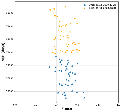
Figure 3: The relationship between MJD and phase for the bursts observed by CHIME after folding with two different $\dot{P}$. The bursts observed by CHIME are folded with Equation (2). The blue points represents the prior 56 bursts and the orange points represents the subsequent 55 bursts. The top panel shows an acceptable example with a period of 16.33 days and a $\dot{P}$ of $1.0\times 10^{-5}$ day day^-1. The bottom panel shows an unacceptable example with a period of 16.33 days and a $\dot{P}$ of $8.6\times 10^{-5}$ day day^-1. We can see in the bottom panel that the active window has a phase shift over time.

3 Constraint on the periodic models

3.1 The Binary models

With current observational data, we can test the periodic models for FRB 20180916B. First, the binary model is considered. The binary model explains the 16-day periodicity by the orbital period, while the 5-day active window can be attributed to the free-free absorption of the companion star wind (Lyutikov et al., 2020; Ioka & Zhang, 2020; Wada et al., 2021). We compile the bursts from recent observations detected by CHIME (CHIME/FRB Collaboration et al., 2019; Chime/Frb Collaboration et al., 2020; Mckinven et al., 2023), LOFAR (Gopinath et al., 2023) and Effelsberg radio telescope (Bethapudi et al., 2023). The bursts detected by Effelsberg radio telescope can expand the frequency to 8 GHz. In Figure 4, we show the relationship between phase and active windows for bursts detected by different telescopes. The period used for folding is 16.33 days, which is the best result with the epoch-folding method. We can see that the active window is narrower and earlier at higher frequencies. Because the higher frequency FRBs are less likely obscured by the companion star wind, this model predicts a narrower active window in lower frequency, which contradicts the chromatic activity discussed above (Pastor-Marazuela et al., 2021; Pleunis et al., 2021b). However, a revised binary model was proposed, which explains the chromatic activity of FRB 20180916B with the intrinsic emission mechanism (Wada et al., 2021). The binary model predicts that the DM of bursts varies within the active windows (Wada et al., 2021; Lyutikov et al., 2020; Ioka & Zhang, 2020). So, we perform the analysis of DM variance in different phases to test this prediction. We use all the bursts provided by CHIME and divide them into three bins with the same phase width. The value of $F$ distribution $F(2,108)=0.045$ and the $p$ value $p=0.95$ are derived, where 2 and 108 in $F(2,108)$ represent the degrees of freedom for $F$ distribution and $p$ represents the possibility to accept the null hypothesis. In this case, the null hypothesis of this analysis is that the mean value of DM for the three phase bins is the same. The $p=0.95$ indicates that the phase is unrelated to the DM of bursts, which contradicts the prediction of this model.

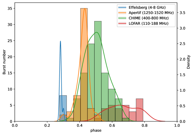
Figure 4: Chromatic periodic activity for different telescopes: Effelsberg (Bethapudi et al., 2023) (blue), Apertif (Pastor-Marazuela et al., 2021) (orange), CHIME (CHIME/FRB Collaboration et al., 2019; Chime/Frb Collaboration et al., 2020; Mckinven et al., 2023) (green) and LOFAR (Pastor-Marazuela et al., 2021; Pleunis et al., 2021a) (red). The period used for the folding is 16.33 days, which is the best-fitting result with epoch-folding method. The colored lines are kernel density estimations. The active window is narrower and earlier at higher frequencies up to 8 GHz.

3.2 The free precession model

Another explanation of the 16.3-day period is the free precession of a neutron star (Levin et al., 2020; Zanazzi & Lai, 2020). The five-day active window requires a fixed emission region, which can be explained by a dipole displaced from the neutron star center. The chromatic activity is attributed to the curvature radiation whose characteristic frequency is dependent on the altitude (Li & Zanazzi, 2021). This model predicts an increase of the period of FRB 20180916B over time due to the loss of mechanical energy (Katz, 2021; Wei et al., 2022). Although there is no obvious increasing trend for the period of FRB 20180916B, the lifetime of free precession derived from the error bar of $\dot{P}$ is still in an acceptable range. However, there is another constraint on the internal magnetic field of the neutron star.

Considering a neutron star exhibiting free precession, its free precession period is related to its rotational period as (Zanazzi & Lai, 2020)

$$P_{\mathrm{pre}}=\frac{P_{\mathrm{rot}}}{\epsilon\cos\theta}.$$ (3)

Here, $\theta$ is the angle between the rotation axis and the maximum moment of inertia and $P_{\mathrm{pre}}$ is the period of precession. $P_{\mathrm{rot}}$ represents the spin period of the neutron star. $\epsilon$ is the ellipticity. In the scenario of the free precession model, the neutron star is deformed by the internal magnetic field $B_{\mathrm{int}}$ (Zanazzi & Lai, 2020)

$$\epsilon=\beta\frac{R^{4}_{\mathrm{ns}}B^{2}_{\mathrm{int}}}{GM^{2}_{\mathrm{ns}}}.$$ (4)

Here, $\beta$ is a constant depending on the topology of the magnetic field and typically we have $|\beta|\ll 1$ (Zanazzi & Lai, 2020). $M_{\mathrm{ns}}$ is the mass of the neutron star which is set as $1.4$ $M_{\odot}$, $R_{\mathrm{ns}}$ is the radius of the neutron star which is set as $10$ km and $G$ is the gravitational constant.

With time going by, the precession period will increase due to the dissipation of mechanical energy. The period derivation can be given by (Katz, 2021)

$$\dot{P}_{\mathrm{pre}}=\frac{P_{\mathrm{pre}}}{t_{\mathrm{sd}}},$$ (5)

where $t_{\mathrm{sd}}$ is the spin-down age which serves as an upper limit for the actual age of precession as discussed before (Katz, 2021). The spin-down age $t_{\mathrm{sd}}$ can be determined by the dipole field $B_{\mathrm{dip}}$ (Zanazzi & Lai, 2020)

$$t_{\mathrm{sd}}=\frac{12c^{3}M_{\mathrm{ns}}}{5B^{2}_{\mathrm{dip}}R^{4}_{\mathrm{ns}}\Omega^{2}_{\mathrm{rot}}},$$ (6)

where $\Omega_{\mathrm{rot}}$ is the angular frequency of the rotation and $c$ is the speed of light. By combining the Equation (3), Equation (5) and Equation (6), we can get (Wei et al., 2022)

$$B_{\mathrm{dip}}=\epsilon\cos\theta\sqrt{\frac{3c^{3}M_{\mathrm{ns}}P^{3}_{\mathrm{pre}}|\dot{\Omega}_{\mathrm{pre}}|}{5\pi^{3}R_{\mathrm{ns}}^{4}}}.$$ (7)

By combining Eqs. (4) and (7) and considering the relationship $B_{\mathrm{dip}}\sim 0.1B_{\mathrm{int}}$ which is commonly employed (Katz, 2021; Wei et al., 2022), we can get $B_{\mathrm{int}}$ with $\dot{P}_{\mathrm{pre}}$ (Wei et al., 2022)

$$B_{\mathrm{int}}=\frac{G}{10\beta R^{2}_{\mathrm{ns}}\cos\theta}\sqrt{\frac{5\pi^{2}M^{3}_{\mathrm{ns}}}{6c^{3}P_{\mathrm{pre}}\dot{P}_{\mathrm{pre}}}}.$$ (8)

With this equation, we show the relationship between $B_{\mathrm{int}}$ and $\dot{P}_{\mathrm{pre}}$ in Figure 5. With the upper limit of $\dot{P}_{\mathrm{pre}}$ derived above, the lower limit of $B_{\mathrm{int}}$ can be given. Astro-Rivelatore Gamma a Immagini Leggero (AGILE) and Swift observed the source of FRB 20180916B in X-ray and $\gamma$-ray bands (Tavani et al., 2020). They detected no extended X-ray and $\gamma$-ray emission, and gave an upper limit of the internal magnetic field (Tavani et al., 2020; Wei et al., 2022), estimated to be in the range of $10^{13.5}-10^{14.5}$G. Here, with the conservative value $\cos\theta<1$, $\beta<0.1$ and $\dot{P}_{\mathrm{pre}}<3.0\times 10^{-5}$ day day^-1, we have $B_{\mathrm{int}}>8.32\times 10^{14}$ G, shown in the green part of Figure 5. It well exceeds the upper limit of $B_{\mathrm{int}}=10^{14.5}$G given by the X-ray and $\gamma$-ray observation (Tavani et al., 2020) as shown in the red part of Figure 5. So the free precession model cannot explain the active period.

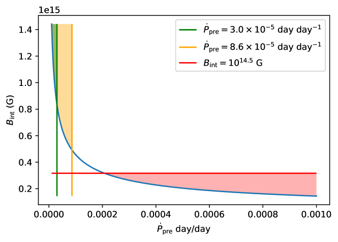
Figure 5: Constraint on the internal magnetic field $B_{\mathrm{int}}$ and period derivative $\dot{P}_{\mathrm{pre}}$ for the free precession model. The Bule line shows the relationship between $B_{\mathrm{int}}$ and $\dot{P}_{\mathrm{pre}}$ from Equation (8). The orange line represents the $\dot{P}_{\mathrm{pre}}=8.6\times 10^{-5}$ day day^-1 and the orange area shows the acceptable value for $\dot{P}_{\mathrm{pre}}$. The green line represents the $\dot{P}_{\mathrm{pre}}=3.0\times 10^{-5}$ day day^-1 and the green area shows the acceptable value for $\dot{P}_{\mathrm{pre}}$. The red line shows the $B_{\mathrm{int}}=10^{14.5}$ G and the red area represents the allowable region for the upper limit given by X-ray and $\gamma$-ray observation (Tavani et al., 2020).

3.3 The forced precession model

Forced precession of a neutron star is another model proposed to explain the period of FRB 20180916B. One of the forced precession models is the orbit-induced spin precession model (Yang & Zou, 2020), in which the FRB source possesses a precession due to the influence of a companion around it. The precession frequency angular $\Omega_{\mathrm{pre}}$ can be derived as (Yang & Zou, 2020)

$$\Omega_{\mathrm{pre}}=\frac{(4+3q)GL}{2a^{3}c^{2}(\sqrt{1-e^{2}})^{3}},$$ (9)

where $q=\frac{M_{1}}{M_{2}}$ and $M_{2}$ is the mass of the neutron star and $M_{1}$ is the mass of the companion. $L$ is the orbital angular momentum:

$$L=\frac{M_{1}M_{2}}{M_{1}+M_{2}}a^{2}\sqrt{\frac{G(M_{1}+M_{2})}{a^{3}}}\sqrt{1-e^{2}},$$ (10)

where $a$ is the semimajor axis of the binary and $e$ is the eccentricity of the binary. We set $e=0$ which was used before (Yang & Zou, 2020; Wei et al., 2022). In this scenario, the precession period is decreasing due to the radiation of gravitational waves,

$$-\frac{dE}{dt} =\frac{32GM_{1}^{2}M_{2}^{2}(M_{1}+M_{2})}{5c^{5}R^{5}},$$ (11)

$$E =-\frac{GM_{1}M_{2}}{2a}.$$ (12)

Here, we assume the initial period as 16.33 days which is the best fitting result as discussed above and calculate the period after evolution of four years for different mass ratios $q$. Then by comparing with the $\dot{P}_{\mathrm{pre}}$ we get above, we have $q>0.3$ as shown in Figure 6.

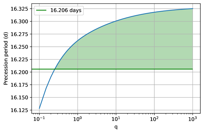
Figure 6: The relationship between mass ratio $q$ and the period after the evolution of four years for orbit-induced spin model. The initial period is set as 16.33 days which is the best fitting results. The blue line shows the period after the evolution of four years as a function of mass ratio $q$. The green line shows the period of 16.206 days which is the temporal results of $\dot{P}_{\mathrm{pre}}=-8.5\times 10^{-5}$ day day^-1. The green area are the acceptable range for mass ratio $q$.

For the fall-back disk model, the neutron star will precess when the rotation axis becomes misaligned with the normal axis of the fall-back disk (Tong et al., 2020):

$$\Omega_{\mathrm{pre}} =\frac{9\epsilon}{4}\frac{M_{\theta}}{M_{\mathrm{ns}}\kappa^{3}}\Omega_{\mathrm{rot}},$$ (13)

$$M_{\theta} =M_{0}\cos\theta_{\mathrm{fb}},$$ (14)

where $M_{0}$ is the total mass of the fall-back disk and $\theta_{\mathrm{fb}}$ is the angle between the rotational axis and the normal direction of a fall-back disk. $\kappa$ is a dimensionless parameter can be set as 1 (Tong et al., 2020; Wei et al., 2022). The evolution of $M_{0}$ can be neglected, so (Wei et al., 2022)

$$\dot{\Omega}_{\mathrm{pre}} =\frac{9\epsilon}{4}\frac{M_{\theta}}{M_{\mathrm{ns}}\kappa^{3}}\dot{\Omega}_{\mathrm{rot}},$$ (15)

$$\dot{\Omega}_{\mathrm{rot}} =\frac{\sin^{2}\theta}{t_{\mathrm{sd}}}\Omega_{\mathrm{rot}}.$$ (16)

where $\theta$ is the angle between the rotational axis and the precession axis. With the two equations and with $|\dot{P}_{\mathrm{pre}}|\leq 8.5\times 10^{-5}$ day day^-1, we can get

$$B_{\mathrm{int}}\geq 8.41\times 10^{14}\mathrm{G}|\sin\theta|\frac{0.1M_{\odot}}{M_{0}\cos\theta_{\mathrm{fb}}},$$ (17)

Since there are many uncertain parameters, the fall-back disk model can not be constrained by the internal magnetic field.

However, the phenomenon that the centers of the active windows for different frequency bands are in different phases is challenging in the context of the forced precession models (Li & Zanazzi, 2021). As shown in Figure 7, the active windows of the forced precession models for different frequency bands show no phase shift, which contradicts previous observations (Li & Zanazzi, 2021).

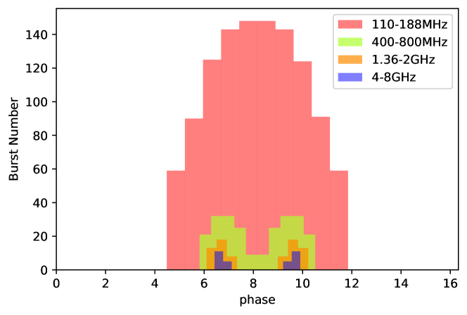
Figure 7: The predicted burst numbers of forced precession model for different frequency bands: 110-188MHz (red), 400-800MHz (green), 1.36-2GHz (orange) and 4-8GHz (blue) under the assumption that the FRBs are emitted due to the curvature radiation. The frequency bands given in this figure are consistent with the frequency bands of LOFAR (Pastor-Marazuela et al., 2021; Pleunis et al., 2021a), CHIME (CHIME/FRB Collaboration et al., 2019; Chime/Frb Collaboration et al., 2020; Mckinven et al., 2023), Apertif (Pastor-Marazuela et al., 2021) and Effelsberg (Bethapudi et al., 2023).

3.4 The ultra-luminous X-ray binary model

Except the neutron star, FRBs can be also generated from an ultra-luminous X-ray binary, in which there are a compact object and a companion star undergoing sustained super-Eddington accretion (Katz, 2020; Sridhar et al., 2021). In this case, the 16-day period can be attributed to the precession of the compact object. The chromatic activity may result from the curvature of the quiescent jet cavity due to the motion of the disk winds driven by precession motion. However, in order to explain the extremely high luminosity of FRBs, the system must undergo unstable mass transfer whose lifetime is about (5-100)$P_{\mathrm{orb}}$ (Sridhar & Metzger, 2022). For a 16-day precession period, the $P_{\mathrm{orb}}$ is less than one day, which means the lifetime of the system is less than 100 days and this is much less than the active duration of FRB 20180916B. Another difficulty is the evolution of RM. This model predicts that the $|$RM$|$ of bursts decreases when the DM also decreases (Sridhar & Metzger, 2022). However, the observed data shows a decreasing trend in the $|$RM$|$ of the bursts, while the DM of bursts remains constant.

3.5 The ultra-long rotation model

For the ultra-long rotation model, the period of FRB 20180916B is considered as the rotational period of a neutron star. The spin down of the rotation is enhanced due to the particle winds or a fallback accretion. So the neutron star can still possess strong magnetic field to power FRBs (Beniamini et al., 2020). The phase shift and different width of active window for different frequency bands can be explained by the the curvature radiation of a displaced dipole consistent with the explanation of free precession above (Li & Zanazzi, 2021). The period of rotation will freeze (Beniamini et al., 2020) which is consistent with the $\dot{P}$ derived from observation. Although it has been not found a neutron star with such a long rotational period, recently two observations reported their discovery of ultra-long period magnetars (Beniamini et al., 2023) and radio transient (Hurley-Walker et al., 2023), which extended the population of radio transients with ultra-long period. PSR J0901-4046 was found to have a period of of 76 s (Caleb et al., 2022) and GLEAM-X J162759.5 was argued to be a magnetar with a period of 1091 s (Hurley-Walker et al., 2022). Recently, a 21-min period radio transient GPMJ1839-10 was reported (Hurley-Walker et al., 2023). Therefore, the discovery of neutron stars with ultra-long rotational periods is promising in the future.

With the help of the Hubble Space Telescope and 10.4 m Gran Telescope Canarias, an optical and infrared imaging as well as integral field spectroscopy observations were presented on FRB 20180916B (Tendulkar et al., 2021). These observations suggest that the source of FRB 20180916B is 250 pc away from the nearest young stellar clump where there are lack of stars to create a magnetar (Tendulkar et al., 2021). If the neutron star is born in the star-forming region and travels to the place of FRB 20180916B, it will need 800 kyr to 7 Myr which exceeds the active age of neutron stars of 10 kyr. However, there still exits the possibility to create a neutron star in the place of FRB 20180916B. Firstly, a compact-binary mergers or accretion-induced collapse can substitute for the core collapse of a massive star to create a neutron star (Margalit et al., 2019; Wang et al., 2020). In addition, a B star ejected from the dense stellar cluster can possess high velocities ($>30$ km s^-1) through binary interactions. With this velocity, the B star is able to move to the region of FRB 20180916B and produce the neutron star with a supernova explosion. Because of that, utilizing a neutron star as the source of FRB 20180916B is still possible.

3.6 A self-consistent model for FRB 20180916B

Another crucial feature of FRB 20180916B is the increase of the RM with the stability of DM in the meanwhile. This phenomenon is difficult to explain in the context of the ultra-long rotation model. For isolated neutron stars, the value of RM is stable. Below, we propose a self-consistent model for FRB 20180916B as shown in Figure 8, which can accommodate the wealth of observational features for FRB 20180916, especially the periodic activity and RM variation. We consider a massive binary containing a slowly rotational neutron star and a massive star with large mass loss. Radio bursts are possibly generated in the magnetosphere through curvature radiation (Yang & Zhang, 2018; Lu et al., 2020). The period can be caused by the ultra-long rotation, and the variation of RM is attributed to the mass loss of the massive star. Within this model, RM variations are caused by the interaction between the radio signal and the magnetized decretion disk or stellar wind during periastron passage of the neutron star. An interacting binary system featuring a magnetar and high-mass stellar star had been proposed to explain the RM variations of FRB 20201124A (Wang et al., 2022) and FRB 20190520B (Wang et al., 2022; Anna-Thomas et al., 2023). In this scenario, the variation of RM is unrelated to the period (Zhao et al., 2023). For a large space of model parameters, this model can explain the increase of RM and the stability of DM for FRB 20180916B (Zhao et al., 2023). In this model, the variation of RM is also periodic, which can be tested by future observations, especially the CHIME telescope.

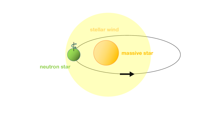
Figure 8: The Schematic diagram of the self-consistent model for FRB 20180916B. The green cricle corresponds to the neutron star with a ultra-long rotation period. The orange circle represents the massive star with stellar wind shown as yellow part. The 16-day period is due to the ultra-long rotation of the neutron star and the variation of the RM is attributed to the orbital motion of this binary system.

4 Conclusions

In this work, we calculate the period and $\dot{P}$ with the bursts detected by CHIME and LOFAR in Sec 2 and find the period keep stable over time. Then, we use the observational data to constrain the periodic model for FRB 20180916B. We find the ultra-long rotation model appears to be the best-fit periodic model for FRB 20180916B. However, the previous ultra-long rotation model considers an isolated neutron star which contradicts the recent observation of RM. So we propose a self-consistent model, which is a massive binary containing a slowly rotational neutron star and a massive star with large mass loss. This modified model can naturally accommodate the wealth of observational features for FRB 20180916B. Moreover, the RM variation of this model is periodic, which can be tested by future observations.

References

- Anna-Thomas et al. (2023) Anna-Thomas, R., Connor, L., Dai, S., et al. 2023, Science, 380, 599, doi: 10.1126/science.abo6526
- Barkov & Popov (2022) Barkov, M. V., & Popov, S. B. 2022, MNRAS, 515, 4217, doi: 10.1093/mnras/stac1562
- Beniamini et al. (2023) Beniamini, P., Wadiasingh, Z., Hare, J., et al. 2023, MNRAS, 520, 1872, doi: 10.1093/mnras/stad208
- Beniamini et al. (2020) Beniamini, P., Wadiasingh, Z., & Metzger, B. D. 2020, MNRAS, 496, 3390, doi: 10.1093/mnras/staa1783
- Bethapudi et al. (2023) Bethapudi, S., Spitler, L. G., Main, R. A., Li, D. Z., & Wharton, R. S. 2023, MNRAS, 524, 3303, doi: 10.1093/mnras/stad2009
- Bochenek et al. (2020) Bochenek, C. D., Ravi, V., Belov, K. V., et al. 2020, Nature, 587, 59, doi: 10.1038/s41586-020-2872-x
- Caleb et al. (2022) Caleb, M., Heywood, I., Rajwade, K., et al. 2022, Nature Astronomy, 6, 828, doi: 10.1038/s41550-022-01688-x
- CHIME/FRB Collaboration et al. (2019) CHIME/FRB Collaboration, Andersen, B. C., Bandura, K., et al. 2019, ApJ, 885, L24, doi: 10.3847/2041-8213/ab4a80
- Chime/Frb Collaboration et al. (2020) Chime/Frb Collaboration, Amiri, M., Andersen, B. C., et al. 2020, Nature, 582, 351, doi: 10.1038/s41586-020-2398-2
- CHIME/FRB Collaboration et al. (2020) CHIME/FRB Collaboration, Andersen, B. C., Bandura, K. M., et al. 2020, Nature, 587, 54, doi: 10.1038/s41586-020-2863-y
- Cordes & Chatterjee (2019) Cordes, J. M., & Chatterjee, S. 2019, ARA&A, 57, 417, doi: 10.1146/annurev-astro-091918-104501
- Cruces et al. (2021) Cruces, M., Spitler, L. G., Scholz, P., et al. 2021, MNRAS, 500, 448, doi: 10.1093/mnras/staa3223
- Dai & Zhong (2020) Dai, Z. G., & Zhong, S. Q. 2020, ApJ, 895, L1, doi: 10.3847/2041-8213/ab8f2d
- Gopinath et al. (2023) Gopinath, A., Bassa, C. G., Pleunis, Z., et al. 2023, arXiv e-prints, arXiv:2305.06393, doi: 10.48550/arXiv.2305.06393
- Gu et al. (2020) Gu, W.-M., Yi, T., & Liu, T. 2020, MNRAS, 497, 1543, doi: 10.1093/mnras/staa1914
- Hurley-Walker et al. (2022) Hurley-Walker, N., Zhang, X., Bahramian, A., et al. 2022, Nature, 601, 526, doi: 10.1038/s41586-021-04272-x
- Hurley-Walker et al. (2023) Hurley-Walker, N., Rea, N., McSweeney, S. J., et al. 2023, Nature, 619, 487, doi: 10.1038/s41586-023-06202-5
- Ioka & Zhang (2020) Ioka, K., & Zhang, B. 2020, ApJ, 893, L26, doi: 10.3847/2041-8213/ab83fb
- Katz (2020) Katz, J. I. 2020, MNRAS, 494, L64, doi: 10.1093/mnrasl/slaa038
- Katz (2021) —. 2021, MNRAS, 502, 4664, doi: 10.1093/mnras/stab399
- Kurban et al. (2022) Kurban, A., Huang, Y.-F., Geng, J.-J., et al. 2022, ApJ, 928, 94, doi: 10.3847/1538-4357/ac558f
- Levin et al. (2020) Levin, Y., Beloborodov, A. M., & Bransgrove, A. 2020, ApJ, 895, L30, doi: 10.3847/2041-8213/ab8c4c
- Li & Zanazzi (2021) Li, D., & Zanazzi, J. J. 2021, ApJ, 909, L25, doi: 10.3847/2041-8213/abeaa4
- Li et al. (2021) Li, Q.-C., Yang, Y.-P., Wang, F. Y., et al. 2021, ApJ, 918, L5, doi: 10.3847/2041-8213/ac1922
- Lorimer et al. (2007) Lorimer, D. R., Bailes, M., McLaughlin, M. A., Narkevic, D. J., & Crawford, F. 2007, Science, 318, 777, doi: 10.1126/science.1147532
- Lu et al. (2020) Lu, W., Kumar, P., & Zhang, B. 2020, MNRAS, 498, 1397, doi: 10.1093/mnras/staa2450
- Lyutikov et al. (2020) Lyutikov, M., Barkov, M. V., & Giannios, D. 2020, ApJ, 893, L39, doi: 10.3847/2041-8213/ab87a4
- Marcote et al. (2020) Marcote, B., Nimmo, K., Hessels, J. W. T., et al. 2020, Nature, 577, 190, doi: 10.1038/s41586-019-1866-z
- Margalit et al. (2019) Margalit, B., Berger, E., & Metzger, B. D. 2019, ApJ, 886, 110, doi: 10.3847/1538-4357/ab4c31
- Mckinven et al. (2023) Mckinven, R., Gaensler, B. M., Michilli, D., et al. 2023, ApJ, 950, 12, doi: 10.3847/1538-4357/acc65f
- Nimmo et al. (2021) Nimmo, K., Hessels, J. W. T., Keimpema, A., et al. 2021, Nature Astronomy, 5, 594, doi: 10.1038/s41550-021-01321-3
- Pastor-Marazuela et al. (2021) Pastor-Marazuela, I., Connor, L., van Leeuwen, J., et al. 2021, Nature, 596, 505, doi: 10.1038/s41586-021-03724-8
- Pleunis et al. (2021a) Pleunis, Z., Michilli, D., Bassa, C. G., et al. 2021a, ApJ, 911, L3, doi: 10.3847/2041-8213/abec72
- Pleunis et al. (2021b) —. 2021b, ApJ, 911, L3, doi: 10.3847/2041-8213/abec72
- Rajwade et al. (2020) Rajwade, K. M., Mickaliger, M. B., Stappers, B. W., et al. 2020, MNRAS, 495, 3551, doi: 10.1093/mnras/staa1237
- Sand et al. (2023) Sand, K. R., Breitman, D., Michilli, D., et al. 2023, arXiv e-prints, arXiv:2307.05839, doi: 10.48550/arXiv.2307.05839
- Sridhar & Metzger (2022) Sridhar, N., & Metzger, B. D. 2022, ApJ, 937, 5, doi: 10.3847/1538-4357/ac8a4a
- Sridhar et al. (2021) Sridhar, N., Metzger, B. D., Beniamini, P., et al. 2021, ApJ, 917, 13, doi: 10.3847/1538-4357/ac0140
- Tavani et al. (2020) Tavani, M., Verrecchia, F., Casentini, C., et al. 2020, ApJ, 893, L42, doi: 10.3847/2041-8213/ab86b1
- Tendulkar et al. (2021) Tendulkar, S. P., Gil de Paz, A., Kirichenko, A. Y., et al. 2021, ApJ, 908, L12, doi: 10.3847/2041-8213/abdb38
- Thornton et al. (2013) Thornton, D., Stappers, B., Bailes, M., et al. 2013, Science, 341, 53, doi: 10.1126/science.1236789
- Tong et al. (2020) Tong, H., Wang, W., & Wang, H.-G. 2020, Research in Astronomy and Astrophysics, 20, 142, doi: 10.1088/1674-4527/20/9/142
- Wada et al. (2021) Wada, T., Ioka, K., & Zhang, B. 2021, ApJ, 920, 54, doi: 10.3847/1538-4357/ac127a
- Wang et al. (2020) Wang, F. Y., Wang, Y. Y., Yang, Y.-P., et al. 2020, ApJ, 891, 72, doi: 10.3847/1538-4357/ab74d0
- Wang et al. (2022) Wang, F. Y., Zhang, G. Q., Dai, Z. G., & Cheng, K. S. 2022, Nature Communications, 13, 4382, doi: 10.1038/s41467-022-31923-y
- Wei et al. (2022) Wei, Y.-J., Zhao, Z.-Y., & Wang, F.-Y. 2022, A&A, 658, A163, doi: 10.1051/0004-6361/202142321
- Xiao et al. (2021) Xiao, D., Wang, F., & Dai, Z. 2021, Science China Physics, Mechanics, and Astronomy, 64, 249501, doi: 10.1007/s11433-020-1661-7
- Yang & Zou (2020) Yang, H., & Zou, Y.-C. 2020, ApJ, 893, L31, doi: 10.3847/2041-8213/ab800f
- Yang & Zhang (2018) Yang, Y.-P., & Zhang, B. 2018, ApJ, 868, 31, doi: 10.3847/1538-4357/aae685
- Zanazzi & Lai (2020) Zanazzi, J. J., & Lai, D. 2020, ApJ, 892, L15, doi: 10.3847/2041-8213/ab7cdd
- Zhang (2023) Zhang, B. 2023, Reviews of Modern Physics, 95, 035005, doi: 10.1103/RevModPhys.95.035005
- Zhao et al. (2023) Zhao, Z. Y., Zhang, G. Q., Wang, F. Y., & Dai, Z. G. 2023, ApJ, 942, 102, doi: 10.3847/1538-4357/aca66b