Deep Learning Approach to Photometric Redshift Estimation

Abstract

Photometric redshift estimation plays a pivotal role in modern astronomy, enabling the determination of celestial object distances by analyzing their magnitudes across various wavelength filters. This study leveraged a dataset of 50,000 objects sourced from the Sloan Digital Sky Survey (SDSS), encompassing magnitudes in five distinct bands alongside their corresponding redshift labels. Traditionally, redshift prediction relied on the use of spectral distribution templates (SED), which, while effective, pose challenges due to their cost and limited availability, particularly when dealing with extensive datasets. This paper explores innovative data-driven methodologies as an alternative to template-based predictions. By employing both a decision tree regression model and a Fully Connected Neural Network (FCN) for analysis, the study reveals a notable discrepancy in performance. The FCN outperforms the decision tree regressor significantly, demonstrating a notable improvement in root mean square error (RMSE) compared to the decision tree. This improvement highlights the FCN’s ability to effectively capture complex relationships within space data. The potential of data-driven redshift estimation is underscored, positioning it as a valuable tool for advancing astronomical surveys and enhancing our comprehension of the universe. With the adaptability to either replace or complement template-based methods, FCNs are poised to reshape the field of photometric redshift estimation, opening up new possibilities for precision and discovery in astronomy.

I Introduction

Photometric redshift estimation is an essential process in modern astronomy, determining the redshift of celestial objects, such as galaxies, stars, and quasars. By measuring the object’s magnitude in different wavelength filters, such as ultraviolet (u) or green (g) and evaluating the differences in magnitude to determine the object’s color (u-g), we can use color values can help estimate redshift for the celestial object [1]. Such estimations play a pivotal role in the interpretation and understanding of large astronomical data surveys, shedding light on distances for celestial objects. Acquiring accurate redshift data is imperative towards advancing our grasp on galaxy formation and evolution.

Traditional methods often employ spectroscopy to determine redshift, utilizing galaxy spectral signature and wavelength shifts. However, this technique can be resource-intensive and expensive. Furthermore, faint celestial objects can pose challenges to spectroscopic observations. These drawbacks have led to the emergence of photometric redshift as a viable alternative. Photometric redshift estimation harnesses the magnitude of extragalactic objects as observed across multiple filters [2]. Rather than relying on a detailed spectrum, astronomers utilize the intensity of light across select broad wavelength bands to infer redshift.

In the realm of galaxy evolution studies, the performance of photometric redshifts (photo-z’s) has profound implications. With systematic uncertainties in modeling galaxy evolution anticipated to persist in the foreseeable future, ensuring the precision of photometric redshift becomes even more important. For instance, the subdivision of objects according to their redshifts is instrumental in targeting specific redshift ranges in spectroscopic surveys. The overarching takeaway is clear: the efficacy of photo-z estimation is integral to the success of galaxy evolution studies. Creating a model that estimates photometric redshift given magnitude data is an optimal tool to assist many areas of research within the astronomical world.

Previous studies have found significant advancements. The CANDELS GOODS-S survey, utilizing the Hubble Space Telescope (HST) Wide Field Camera 3 (WFC3) H-band and Advanced Camera for Surveys (ACS) z-band, has helped expand our understanding of photometric redshifts [3]. This dataset, with TFIT photometry, explored the efficacy of various codes and template Spectral Energy Distributions. It found that methods which incorporated training using a spectroscopic sample achieved enhanced accuracy. Importantly, the research found a direct correlation between the source magnitude and the precision of redshift estimation, emphasizing the role of magnitude in estimation.

Another approach was utilizing Bayesian methodologies [4]. By employing prior probabilities and Bayesian marginalization, this method was adept at utilizing previously overlooked data like the expected shape of redshift distributions and galaxy type fractions. When applied to B130 HDF-N spectroscopic redshifts, this Bayesian approach showcased promising results, reinforcing its potential to address existing gaps. Importantly, these advancements were realized without the reliance on a training-set procedure, while utilizing template libraries.

Both studies used template Spectral Energy Distribution (SED) data to help test their different methodologies. While template SEDs do help estimate photometric redshift, it’s become increasingly more difficult to obtain these distributions with larger datasets. Given the next generation of surveys from the James Webb Space Telescope (JWST) and Rubin Observatory (LSST), photometric redshift estimation needs a more data-driven approach to accurately predict redshift based on observational data [5].

The primary objective of this paper is to explore novel computational methods that take a data-driven approach to estimation, while increasing accuracy. A data-driven approach involves relying on actual observational data, such as magnitude or flux values, rather than theoretical template SEDs. Specifically, this research aims to evaluate the reliability of Fully Connected Neural Networks (FCN) in estimating photometric redshift using magnitude data. Recent advancements in the field of machine learning have opened up new opportunities to utilize novel methods such as artificial neural networks. Fully Connected Neural Networks, a subset of artificial neural networks, are designed to capture complex relationships in data, increasing overall predictive abilities for a model [6].

Despite the clear capabilities for neural network applications in astronomy, there remains a gap in comprehensive studies that use magnitude and color index data to make redshift predictions. Our research seeks to bridge this gap, comparing the Fully Connected Network with a decision tree regressor to see the efficacy of both when provided with light data from the Sloan Digital Sky Survey (SDSS).

We aim to create both a decision tree regression model and FCN for photometric redshift estimation. The scope encompasses the design, training and testing of these models, followed by an analysis of their performance. Comparison metrics between the two methods will be RMS values and overall prediction accuracy.

II Methodology

II-A Data

Our study utilized a dataset from the Sloan Digital Sky Survey [7] with 50,000 celestial objects. For each of the objects, magnitudes of 5 different bands were included in the data. The 5 bands - u,g,r,i,z - represent different wavelengths of light from each galaxy or quasar [8]. Alongside the magnitudes, the dataset came with redshift value labels for each object. These redshifts were obtained from spectroscopic measurements from SDSS (Table 1).

TABLE I: SDSS Dataset: Contains the first five rows of our original dataset for the object’s magnitude in different wavelength filters (u, g, r, i, and z) and the redshift values.

u	g	r	i	z	redshift
18.27449	17.01069	16.39594	16.0505	15.79158	0.0369225
18.51085	17.42787	16.94735	16.61756	16.46231	0.06583611
18.86066	17.91374	17.56237	17.26353	17.13068	0.1202669
19.38744	18.37505	17.63306	17.25172	17.00577	0.1806593
18.38328	16.59322	15.77696	15.3979	15.08755	0.04035749

Before delving into model training and testing, we visualized different portions of the data to better understand the distributions (Fig. 1).

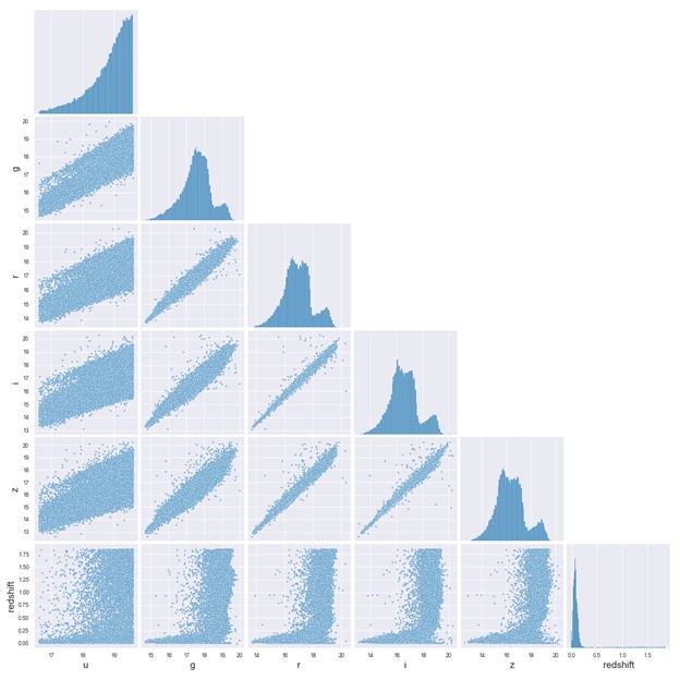
Figure 1: Pair Plot for SDSS Data: The pair plot above shows the correlation between different magnitudes and their redshift values in the dataset. Each respective feature is paired with another and results in a scatterplot displaying the relationship between them.

II-B Preprocessing

We performed sigma-clipping on the redshift values using a sigma value of 3 standard deviations from the mean of the redshift values to remove outliers while retaining 95 percent of the data. The equation for the standard deviation is

$$\sigma=\sqrt{\frac{\sum{(x_{i}-\mu)}^{2}}{N}},$$ (1)

where $\mu$ is the mean of all the redshift values in the dataset, N is the total number of redshift values, and x represents each individual redshift value.

Additionally, we removed redshift values less than zero as these are not physical. As a result, we ended with a dataset of 47,484 celestial objects out of the original 50,000.

II-C Decision Tree Regressor

We compared two methods, a decision tree regressor and a fully connected neural network. The decision tree regressor works by partitioning the datasets into small subsets. Each split is based on the value of the input features. Our features consisted of the 5 bandpass filters (u,g,r,i,z) as well as the colors formed by their magnitude differences (u-g),(g-r),(r-i), and (i-z). After splitting the data, we arrive at leaf nodes where the redshift values are as similar as possible. Each leaf of the tree then predicts the average redshift of the instances that fall into it. The model is simple and transparent.

II-D Fully Connected Neural Network

Our next step was to create a model that could predict the redshift, given our inputs of the object in question. We chose a fully connected neural network that used the Adaptive Moment Estimation Optimizer [9] in order to create a regression model to predict redshift.

Our input layer consists of 9 inputs and an output shape of 100. The 9 inputs are composed of magnitudes across each of the band passes and the magnitude differences as follows,

$${M}_{Input}=[m_{u},m_{g},m_{r},m_{i},m_{u-g},m_{g-r},m_{r-i},m_{i-z}].$$ (2)

We then added two more layers of neurons until the last layer with 65 neutrons and 35 neurons, respectively. With only one neuron in this last layer, it represents the predicted redshift. We used the Rectified Linear Unit (ReLU) activation function [10] which worked better than the sigmoid function to account for redshift predictions with values greater than 1 as well as to improve efficiency of the network. Lastly we added a dropout rate of 0.2 to prevent overfitting after each layer which finalized the composition of the neural network’s architecture (Fig. 2).

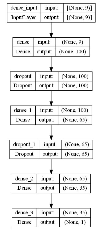
Figure 2: Neural Network Architecture: The chart above shows the layers and dropouts for the neural network and how the model’s neurons are arranged to obtain the redshift value from the nine input parameters.

II-E Loss Function - Mean Squared Error

We minimize the mean squared error as the loss function in our neural network,

$$\mathcal{L}=\frac{1}{n}\sum_{i=1}^{n}{(y-\hat{y})^{2}},$$ (3)

where y is the true redshift, y-hat is the predicted redshift, and n is the number of objects in a batch of the training set.

III Results

For the original decision tree regressor, the RMS value was above 0.16. In addition, when graphing the true redshift values versus the predicted values given by the tree regressor, we see a graph with a lot of noise and many values far from the predicted line (Fig. 3). Using our neural network, we were able to improve accuracy when predicting redshift to 0.009 RMS using the predicted line (y-hat) that our neural network produced (Fig. 4 and Fig. 5).

The improvement in the RMS show that the neural network predictions have improved upon those from the Decision Tree Model (previously used to predict photometric redshift in stars and quasars) due to a lower RMS and lower deviations and discrepancies from predicted redshift to actual redshift as observed in the graphs above (Fig. 4 and Fig. 5).

In addition, the model was trained to prevent overfitting to our dataset, so our results can be generalized to any data in this particular data format, given all nine parameters are present (Fig. 6).

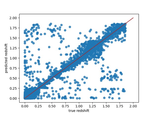
Figure 3: Decision Tree Regressor Scatter Plot: The graph shows true redshift vs predicted redshift correlation for the predictions made by the decision tree regressor.

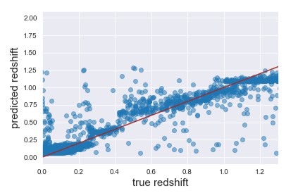
Figure 4: Fully Connected Neural Network Scatter Plot: The graph above shows true redshift vs predicted redshift correlation for the fully connected neural network’s predictions. There are few outliers, with most predictions being close to the best fit line.

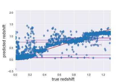
Figure 5: Neural Network Scatter Plot with Error bars: The graph shows error bars (horizontal purple lines) with the true redshift vs predicted redshift graph to give insight on the uncertainties in these predictions made by the fully connected neural network. More specifically, it uses the redshift error parameter values given in the dataset and takes the ones pertaining to the data points shown on the scatter plot.

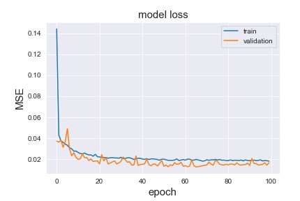
Figure 6: Line Graph showing Epochs vs MSE: This graph shows the learning curve of the fully connected neural network. The loss of the training function followed the same trajectory as that of the validation set, stabilizing, and reaching an equilibrium, indicating a good fit.

IV Conclusion

The implications of the study extend beyond the test dataset. The empirical evidence from our study has not only demonstrated a data-driven approach but has shed light on incredibly efficient methods for photometric redshift estimation. The refined precision of redshift values delivered by our FCN is poised to revolutionize the identification process, ensuring more accurate categorizations for distance estimation of objects.

The strength of our FCN lies in its generalizability and usability. Since it thrives on capturing intricate data relationships, the model can adapt to datasets with varying structures and magnitudes, enhancing its scalability. Furthermore, this broadens the scope of its application, making it suitable for diverse astronomical tasks beyond just redshift estimation.

This shift towards a data-driven methodology holds strong implications for the future of astronomical research. Compared to the traditional decision tree regression models, the FCN showcases a clear edge in estimating redshifts. This distinction becomes paramount when differentiating between quasars and stars. Moreover, as the acquisition of SED templates becomes increasingly challenging, the need for approaches that can efficiently utilize raw astronomical data will become more pressing. Our FCN model, with its strong adaptability and scalability, stands as a testament to the possibilities that lie in store for data-driven astronomy.

Moreover, the refined precision of redshift values produced by our FCN, combined with its adaptability, can significantly improve identification processes in astronomy, ensuring more accurate categorizations even in the absence of traditional SED templates.

Yet, our study does have certain limitations. Despite the vastness of our dataset, 50,000 celestial objects might still just be scratching the surface. The universe’s expanse and the inherent variability within it mean that larger datasets could exhibit different behaviors, and while our FCN is promising, its real test would be in even more diversified astronomical conditions. Additionally, while meticulous data preprocessing was executed, we cannot completely discount its potential influence on the performance metrics of the decision tree regression.

V Future Work

Building on the study’s foundation, there are various options for improvement and future research. Given the success of the FCN, exploring Convolutional Neural Networks could capture spatial patterns in the data that may have been overlooked. The integration of hybrid models, such as combining FCNs with Random Forests would improve overall accuracy. Lastly, fine-tuning pre-trained models would build on the foundation of previous successes to improve predictive power for redshift.

References

- [1] J.A. Newman, D. Gruen, ”Photometric Redshifts for Next-Generation Surveys,” vol.60, Annual Review of Astronomy and Astrophysics, 2022, pp. 363.
- [2] M. Salvato, O. Ilbert, B. Hoyle, ”The many flavours of photometric redshifts,” Cornell Arxiv, June 2018.
- [3] T. Dahlen, et al., “A Critical Assessment of Photometric Redshift Estimation: A CANDELS Investigation,” 2nd issue, vol. 775. The Astrophysical Journal, 2000, pp.93.
- [4] N. Benitez, ”Bayesian Photometric Redshift Estimation,” 2nd issue, vol. 536. The Astrophysical Journal, 2000, pp.571.
- [5] Z. Ivezić, et al.,“LSST: From Science Drivers to Reference Design and Anticipated Data Products,” 2nd issue, vol. 873. The Astrophysical Journal, 2019, pp.111.
- [6] A.G. Schwing, R. Urtasun, ”Fully Connected Deep Structured Networks,” Cornell Arxiv, March 2015.
- [7] J.A. Kollmeier, et al., “SDSS-V: Pioneering Panoptic Spectroscopy,” Cornell Arxiv, November 2017.
- [8] T.K. Wyder, et al., ”The UV-Optical Color Magnitude Diagram. II. Physical Properties and Morphological Evolution On and Off of a Star-forming Sequence,” issue 2, vol.173, The Astrophysical Journal Supplement Series, 2007, pp. 315.
- [9] D.P. Kingma, J. Ba, “Adam: A Method for Stochastic Optimization,” Cornell Arxiv, January 2017.
- [10] A.F. Agarap, “Deep Learning using Rectified Linear Units (ReLU),”, Cornell Arxiv, February 2019.