Private Estimation and Inference in High-
Dimensional Regression with FDR Control

Abstract

This paper presents novel methodologies for conducting practical differentially private (DP) estimation and inference in high-dimensional linear regression. We start by proposing a differentially private Bayesian Information Criterion (BIC) for selecting the unknown sparsity parameter in DP-Lasso, eliminating the need for prior knowledge of model sparsity, a requisite in the existing literature. Then we propose a differentially private debiased LASSO algorithm that enables privacy-preserving inference on regression parameters. Our proposed method enables accurate and private inference on the regression parameters by leveraging the inherent sparsity of high-dimensional linear regression models. Additionally, we address the issue of multiple testing in high-dimensional linear regression by introducing a differentially private multiple testing procedure that controls the false discovery rate (FDR). This allows for accurate and privacy-preserving identification of significant predictors in the regression model. Through extensive simulations and real data analysis, we demonstrate the efficacy of our proposed methods in conducting inference for high-dimensional linear models while safeguarding privacy and controlling the FDR.

Keywords: differential privacy, high dimension, linear regression, debiased Lasso, false discovery rate control.

1 Introduction

In the era of big data, the significance of data privacy has grown considerably. With the continuous collection, storage, processing, and sharing of vast amounts of personal data (Lane et al., 2014), there is a pressing need to protect sensitive information. Traditional data analytics and statistical inference tools, unfortunately, may fall short in ensuring such protection. However, the concept of differential privacy, initially proposed by theoretical computer scientists (Dwork et al., 2006), has made substantial progress and found widespread use in various large-scale applications. In essence, differentially private algorithms incorporate random noise that is independent of the original database and produce privatized summary statistics or model parameters. The ultimate goal of differentially private analysis is to safeguard individual data while still allowing meaningful statistical analysis of the original database.

In this paper, we develop a novel framework that enables differentially private statistical inference in high-dimensional linear regression. Let $Y\in{\mathbb{R}}$ be the response and $X\in{\mathbb{R}}^{p}$ be the covariates. Assume the linear model

$$Y={\bm{\beta}}^{\top}X+e,$$

where $e$ denotes the noise term and follows the sub-Gaussian distribution. Assume that $\{\bm{x}_{i},y_{i}\}_{i=1}^{n}$ are independent samples. We are interested in the high-dimensional setting where $p$ may grow exponentially with $n$, and only a small subset of ${\bm{\beta}}$ have non-zero values. We aim to develop practical differentially private estimation and inference methods for the parameter ${\bm{\beta}}$, and a false discovery rate control procedure when multiple testing is concerned.

Numerous approaches have been developed to address the challenge of statistical inference in high-dimensional linear regression, under the typical non-private setting. Wasserman and Roeder (2009) applied sample-splitting for high-dimensional inference, where the estimation and inference are conducted on different samples. Later on, the debiased lasso (Zhang and Zhang, 2014; Javanmard and Montanari, 2014; Van de Geer et al., 2014) emerged as a technique capable of mitigating the potential bias arising from the Lasso estimator, thereby providing asymptotically optimal confidence intervals for regression coefficients. Additionally, Ning and Liu (2017) proposed a method for constructing confidence intervals for high-dimensional penalized M-estimators based on decorrelated score statistics, while Shi et al. (2021) developed a recursive online-score estimation approach. More recently, Wang et al. (2022) introduced the repro framework, which enables the construction of valid confidence intervals for finite samples with high-dimensional covariates.

Besides conducting inference on one parameter, another desired feature in high dimensional linear regression is to control the false discovery rate (FDR) of the selected variables. This objective has led to the development of various FDR control methods in the literature. One such method, proposed by Liu (2013), focuses on the Gaussian graphical model and utilizes the asymptotic normality of the test statistic (Liu, 2013). Another influential approach is the knockoff framework introduced by Barber and Candès (2015), which exploits the symmetry of the statistics under the null hypothesis. Since its inception, the knockoff method has undergone further development and generalization, finding applications in diverse settings (Candes et al., 2018; Barber and Candès, 2019; Romano et al., 2020). Recently, Dai et al. (2022) proposed a method that combines the idea of symmetric mirror statistics and data splitting to control the FDR asymptotically. The power of this method can be further enhanced by implementing a multiple-split approach. Dai et al. (2023) extended this idea to generalized linear models, expanding its applicability.

Addressing privacy concerns in various statistical inference scenarios has gained significant attention in recent literature. Avella-Medina et al. (2023a) put forth the utilization of first-order and second-order optimization algorithms to develop private M-estimators, and they conducted an analysis of the asymptotic normality of these private estimators, accompanied by an evaluation of their privacy error rate. The extension of these methodologies to the high dimensional setting is further discussed in Avella-Medina et al. (2023b), albeit not published yet. Moreover, the multiple testing problem has also been a subject of recent investigation. Dwork et al. (2021) proposed the DP-BH method, while Xia and Cai (2023) introduced the DP-Adapt method, which provides control over the false discovery rate (FDR) while guaranteeing finite sample performance.

Our paper contributes to the differentially private analysis of high-dimensional linear regression in several key aspects.

1. We propose a differentially private Bayesian Information Criterion (BIC) to accurately select the unknown sparsity parameter in DP-Lasso proposed by Cai et al. (2021), eliminating the need for prior knowledge of the model sparsity. This advancement enhances the reliability of the DP-Lasso framework and can be used in many downstream tasks.

2. We develop a differentially private debiased Lasso procedure which can produce asymptotic normal estimators with privacy. This procedure provides differentially private confidence interval for a single parameter of interest.

3. We design a differentially private procedure for controlling FDR in multiple testing scenarios. Our approach allows for FDR control at any user-specified rate $\alpha$ and exhibits asymptotic power approaching 1 under proper conditions.

The structure of this paper is as follows. In Section 2, we present a formulation of the problem of interest and propose a new estimation of DP-Lasso that do not require the knowledge of sparsity. In Section 3, we introduce the differentially private debiased Lasso algorithm and provide its asymptotic distribution and privacy error. Section 4 presents a novel differentially private false discovery rate (FDR) control method that leverages sample splitting and mirror statistics. We also elucidate the reasons why existing FDR techniques are inapplicable in the context of differential privacy. In Section 5, we present extensive simulations and real data analysis to validate the performance of our proposed methods. Finally, in Section 6, we conclude the article with a discussion of our findings and outline potential future research directions. All proofs are provided in the appendix.

Notation: Throughout the paper, we use the following notation. For any $p$-dimensional vector $\bm{x}=(x_{1},\dots,x_{p})^{\top}$, we define the $l_{q}$-norm of $\bm{x}$ as $\|\bm{x}\|_{q}:=(\sum_{i=1}^{p}|x|_{i}^{q})^{1/q}$ for $1\leq q$, with $|\cdot|$ representing the absolute value. The $\text{supp}(\bm{x})=\{i:|x_{i}|>0\}$ is the index set of nonzero elements in $\bm{x}$. We define the $l_{0}$-norm of $\bm{x}$ by $\|\bm{x}\|_{0}=\#\text{supp}(\bm{x})$, which is number of nonzero coordinates of $\bm{x}$. For a positive integer $n$, we use $[n]$ to denote the set $\{1,\dots,n\}$. For a subset $\mathcal{S}\subseteq[k]$ and vector $\bm{x}\in\mathbb{R}^{n}$, we use $\bm{x}_{\mathcal{S}}$ to denote the restriction of vector $\bm{x}$ to the index set $\mathcal{S}$. For a vector $\bm{x}\in\mathbb{R}^{n}$, we use $\Pi_{R}(\bm{x})$ to denote the projection of $\bm{x}$ onto the $l_{2}$-ball $\{\bm{u}\in\mathbb{R}^{p}:\|\bm{u}\|_{2}\leq R\}$. Let $X$ and $\{X_{n}\}_{n=1}^{\infty}$ be random variables. The expression $X_{n}\xrightarrow{D}X$ denotes the convergence of $X_{n}$ to $X$ in distribution. Similarly, the notation $X_{n}=O_{P}(a_{n})$ indicates that the random variable $X_{n}/a_{n}$ is stochastically bounded.

2 Preliminaries

Consider the dataset $D:=\{(\bm{x}_{i},y_{i})\}_{i=1}^{n}\in\mathcal{D}$ that are drawn from the distributions satisfying

$$y_{i}={\bm{\beta}}^{\top}\bm{x}_{i}+e_{i},$$

where $e_{i}\stackrel{{\scriptstyle i.i.d.}}{{\sim}}N(0,\sigma^{2})$, ${\bm{\beta}}\in{\mathbb{R}}^{p}$ and $\|{\bm{\beta}}\|_{0}\leq s$. In this paper, we are interested in the high-dimensional setting where the dimension $p$ may grow exponentially with the sample size $n$, under the $(\epsilon,\delta)$-differential privacy framework. We begin by introducing the background of differential privacy, with its formal definition as follows.

Definition 1 (Differential Privacy (Dwork et al., 2006)).

A randomized algorithm $M:\mathcal{D}\to\mathcal{R}$ is $(\epsilon,\delta)$-differentially private for $\epsilon,\delta>0$ if for every pair of neighboring data sets $D,D^{\prime}\in\mathcal{D}$ that differ by one individual datum and every measurable set $\mathcal{S}\subset\mathcal{R}$ with respect to $M(\cdot)$,

$$\mathbb{P}[M(D)\in\mathcal{S}]\leq e^{\epsilon}\mathbb{P}[M(D^{\prime})\in\mathcal{S}]+\delta,$$ (2.1)

where the probability measure $\mathbb{P}$ is induced by the randomness of $M$ only.

In the definition, two data sets $D$ and $D^{\prime}$ are treated as fixed, and the probability measures the randomness in the mechanism $M(\cdot)$. The level of privacy against an adversary is controlled by the pre-specified privacy parameters $(\epsilon,\delta)$. When $\epsilon$ and $\delta$ are small, the algorithm offers strong privacy guarantees.

One of the most useful concepts in differential privacy is the sensitivity, which characterizes the magnitude of change in the algorithm when only one single individual in the dataset is replaced by another element.

Definition 2 (Sensitivity).

For a vector-valued deterministic algorithm $\mathcal{T}(\cdot):D\in\mathcal{D}\to{\mathbb{R}}^{m}$, the $l_{q}$ sensitivity of $\mathcal{T}(\cdot)$ is defined as

$$\Delta_{q}(\mathcal{T}):=\sup_{D,D^{\prime}\in\mathcal{D}}\|\mathcal{T}(D)-\mathcal{T}(D^{\prime})\|_{q},$$ (2.2)

where $D$ and $D^{\prime}$ only differ in one single entry.

Next, we introduce two well-known mechanisms: the Laplace mechanism, which is $(\epsilon,0)$ differential privacy for algorithms with bounded $l_{1}$ sensitivity, and the Gaussian mechanism, which achieves $(\epsilon,\delta)$ differential privacy for algorithms with bounded $l_{2}$ sensitivity.

Lemma 1 (Dwork and Roth (2014)).

  

1. (Laplace mechanism): For a deterministic algorithm $\mathcal{T}(\cdot)$ with $l_{1}$ sensitivity $\Delta_{1}(\mathcal{T})$, the randomized algorithm $\mathcal{M}(\cdot):=\mathcal{T}(\cdot)+\bm{\xi}$ achieves $(\epsilon,0)$-differential privacy, where $\bm{\xi}=(\xi_{1},\dots,\xi_{m})^{\top}$ follows i.i.d. Laplace distribution with scale parameter $\Delta_{1}(\mathcal{T})/\epsilon$.

2. (Gaussian mechanism): For a deterministic algorithm $\mathcal{T}(\cdot)$ with $l_{2}$ sensitivity $\Delta_{2}(\mathcal{T})$, the randomized algorithm $\mathcal{M}(\cdot):=\mathcal{T}(\cdot)+\bm{\xi}$ achieves $(\epsilon,\delta)$-differential privacy, where $\bm{\xi}=(\xi_{1},\dots,\xi_{m})^{\top}$ follows i.i.d. Gaussian distribution with mean $0$ and standard deviation $\sqrt{2\log(1.25/\delta)}\Delta_{2}(\mathcal{T})/\epsilon$.

Differentially private algorithms have other nice properties that will be useful for our analysis, as summarized in the following lemma.

Lemma 2.

Differentially private algorithms have the following properties (Dwork et al., 2006, 2010):

1. Post-processing: Let $\mathcal{M}(\cdot)$ be an $(\epsilon,\delta)$-differentially private algorithm and $f(\cdot)$ be a deterministic function that maps $\mathcal{M}(D)$ to real Euclidean space, then $f\{\mathcal{M}(D)\}$ is also an $(\epsilon,\delta)$-differentially private algorithm.

2. Composition: Let $\mathcal{M}_{1}(\cdot)$ be $(\epsilon_{1},\delta_{1})$-differentially private and $\mathcal{M}_{2}(\cdot)$ be $(\epsilon_{2},\delta_{2})$- differentially private, then $\mathcal{M}_{1}\circ\mathcal{M}_{2}$ is $(\epsilon_{1}+\epsilon_{2},\delta_{1}+\delta_{2})$-differentially private.

3. Advanced Composition: Let $\mathcal{M}(\cdot)$ be $(\epsilon,0)$-differentially private and $0<\delta^{\prime}<1$, then $k$-fold adaptive composition of $\mathcal{M}(\cdot)$ is $(\epsilon^{\prime},\delta^{\prime})$-differentially private for $\epsilon^{\prime}=k\epsilon(e^{\epsilon}-1)+\epsilon\sqrt{2k\log(1/\delta^{\prime})}$.

In high-dimensional problems, parameters of interest are often assumed to be sparse. Reporting the entire estimation results can result in a substantial variance. Fortunately, exploiting the sparsity assumption allows us to selectively disclose only the significant nonzero coordinates. The “peeling” algorithm (Dwork et al., 2021) is a differentially private algorithm that addresses this problem by identifying and returning the top-$s$ largest coordinates based on the absolute values. Since its proposal by Dwork et al. (2021), this algorithm has been popular in protecting privacy for high-dimensional data, see for example, applications in Cai et al. (2021) and Xia and Cai (2023).

Input : vector-valued function $\bm{\xi}=\bm{\xi}(D)\in\mathbb{R}^{d}$, sparsity $s$, privacy parameters $\varepsilon,\delta$, noise scale $\lambda$.

1 Initialize $S=\emptyset$;

2 for $i$ in $1$ to $s$ do

3       Generate $\bm{\eta}_{i}\in\mathbb{R}^{d}$ with $\eta_{i1},\eta_{i2},\cdots,\eta_{id}\stackrel{{\scriptstyle\text{i.i.d.}}}{{\sim}}\text{Laplace}\left(\lambda\cdot\frac{2\sqrt{3s\log(1/\delta)}}{\varepsilon}\right)$;

4       Append $j^{*}=\operatorname*{arg\,max}_{j\in[d]\setminus S}|\xi_{j}|+\eta_{ij}$ to $S$;

5      

6 end for

7Set $\tilde{P}_{s}(\bm{v})=\bm{\xi}_{S}$;

8 Generate $\tilde{\bm{\eta}}$ with $\tilde{\eta}_{1},\cdots,\tilde{\eta}_{d}\stackrel{{\scriptstyle\text{i.i.d.}}}{{\sim}}\text{Laplace}\left(\lambda\cdot\frac{2\sqrt{3s\log(1/\delta)}}{\varepsilon}\right)$;

Output : $\tilde{P}_{s}(\bm{\xi})+\tilde{\bm{\eta}}_{S}$.

Algorithm 1 Noisy Hard Thresholding ($NoisyHT(\bm{\xi},s,\epsilon,\delta,\lambda)$)

Lemma 3 (Dwork et al. (2021)).

For a vector-valued function $\bm{v}$ with $\|\bm{v}(D)-\bm{v}(D^{\prime})\|_{\infty}\leq\lambda$, where $D^{\prime}$ is a neighboring data set of $D$, Algorithm 1 is $(\epsilon,\delta)$-differentially private.

3 Differentially Private Estimation

The estimation of regression parameters in the high-dimensional private setting has been studied in Cai et al. (2021) with optimality guarantees. However, the algorithm in Cai et al. (2021) requires prior knowledge of the sparsity parameter $s$, which are typically unknown in practice. In this section, we propose a differentially private Bayesian Information Criterion (BIC) in Algorithm 2 to accurately select the unknown sparsity parameter, eliminating the need for prior knowledge of the model sparsity. The pipeline of the proposed estimation algorithm is as follows.

Input : dataset $\{(\bm{x}_{i},y_{i})\}_{i\in[n]}$, step size $\eta^{0}$, privacy parameters $\varepsilon,\delta$, noise scale $B$, number of iterations $T$, truncation level $R$, feasibility parameter $C$, initial value ${\bm{\beta}}^{(0)}$.

1 Random split data into $T$ parts of roughly equal sizes: $[n]=\mathcal{S}_{0}\cup\dots\cup\mathcal{S}_{T-1}$ and $\mathcal{S}_{i}\cap\mathcal{S}_{j}=\emptyset$ for $i\neq j$;

2Set $K=\lfloor\log_{2}(\sqrt{n}/\log^{2}p)\rfloor$;

3 for $k$ in $0$ to $K$ do

4      $s=2^{k}$ ;

5       for $t$ in $0$ to $T-1$ do

6             Compute ${\bm{\beta}}^{(t+0.5)}={\bm{\beta}}^{(t)}-(\eta^{0}/|\mathcal{S}_{t}|)\sum_{i\in\mathcal{S}_{t}}(\Pi_{R}(\bm{x}_{i}^{\top}{\bm{\beta}}^{(t)})-\Pi_{R}(y_{i}))\bm{x}_{i}$  where $|\mathcal{S}_{t}|$ is the size of set $\mathcal{S}_{t}$; ${\bm{\beta}}^{(t+1)}=\Pi_{C}(\text{NoisyIHT}({\bm{\beta}}^{(t+0.5)},s,\varepsilon/\{T(K+2)\},\delta/\{T(K+1)\},\eta^{0}B/n))$.

7       end for

8      Let $\hat{{\bm{\beta}}}(k)={\bm{\beta}}^{(T)}$.

9 end for

10We select the model based on the BIC type of loss:

$$\hat{{\bm{\beta}}}= \operatorname*{arg\,min}_{\hat{{\bm{\beta}}}(k):0\leq k\leq K}\bigg{\{}\sum_{i=1}^{n}\{\Pi_{R}(y_{i})-\Pi_{R}(\bm{x}_{i}^{\top}\hat{{\bm{\beta}}}(k))\}^{2}+c_{0}\bigg{\{}\log(p)\log(n)\cdot 2^{k}$$

$$+\frac{\log(p)^{2}\cdot 2^{2k}\log(1/\delta)\log^{7}n}{n\epsilon^{2}}\bigg{\}}+z_{k}\bigg{\}},$$

where $z_{k}\stackrel{{\scriptstyle i.i.d.}}{{\sim}}\text{Laplace}\bigg{(}\frac{2(4R)^{2}(K+2)}{\epsilon}\bigg{)}$.

Output : $\hat{\bm{\beta}}$.

Algorithm 2 Adaptive Differentially Private Sparse Linear Regression

The random sample splitting in the proposed algorithm is equivalent to employing the stochastic gradient descent algorithm with one pass of the entire dataset. Moreover, our choice to use the powers of 2 as candidate values of the sparsity parameter accomplishes two critical goals: firstly, it ensures that the candidate set covers the true model by defining an interval where $s$ falls, such that $s^{*}<s<2s^{*}$ where $s^{*}$ is in the candidate set; secondly, it limits the total number of candidate models to $\log n$, which is indeed $o(n)$. The choice of $K=\log_{2}(\sqrt{n}/\log^{2}p)$ aligns with the sparsity requirement for statistical inference, as will be discussed in Section 4.

Condition 3.1.

The covariates ${\bm{x}}_{i}$ are independent sub-Gaussian with mean zero and covariance $\bm{\Sigma}$ such that $1/L\leq\Lambda_{\min}(\bm{\Sigma})\leq\Lambda_{\max}(\bm{\Sigma})\leq L$. There is a constant $c_{x}<\infty$ such that $\|\bm{x}_{i}\|_{\infty}<c_{x}$.

Condition 3.2.

The true parameter satisfies $\|{\bm{\beta}}\|_{2}\leq c_{0}$ for some constant $c_{0}$ and $\|{\bm{\beta}}\|_{0}\leq s$.

Condition 3.1 is commonly assumed in the high-dimensional literature; for example, see Javanmard and Montanari (2014). The bound on the infinity norm of the design matrix $c_{x}$ can be relaxed to hold with high probability, which can be easily obtained for sub-Gaussian distributions. Different from the algorithm proposed by Cai et al. (2021), we employ a data-splitting technique in the algorithm to establish independence between $\bm{\beta}^{(t)}$ and the sub-data $\bm{x}_{i}$ utilized in the $t$-th iteration. Notably, our Condition 3.1 is less stringent than the design conditions outlined in Cai et al. (2021). This reduction in conditions comes at the cost of decreasing the effective sample size by a factor of $1/T$. As demonstrated in Theorem 3.1, the number of iterations, denoted as $T$, adheres to $T=O(\log(n))$, resulting in an associated error bound increase of $O(\log(n))$. Condition 3.2 assumes the bound and sparsity for the true parameter ${\bm{\beta}}$. Lemma 3.1 provides the privacy guarantee of Algorithm 2, where we only require condition 3.1.

Lemma 3.1.

Assume Condition 3.1 and $B\geq 4Rc_{x}$, Algorithm 2 is $(\epsilon,\delta)$-differentially private.

Now we establish the error bound of the new estimation algorithm.

Theorem 3.1.

Suppose Conditions 3.1 and 3.2 hold, and let $R=\sigma\sqrt{2\log n}$, $B=2(R+c_{0}c_{x})c_{x}$ and $C>c_{0}$. There exists a constant $\rho$ such that, if $2^{K}>\rho L^{4}s$, $\eta^{0}=1/6L$, $T=\rho L^{2}\log(8c_{0}^{2}Ln)$, $s\log p\log n=o(n)$ and $s\log p\sqrt{\log(1/\delta)}\log^{3.5}n/\epsilon=o(n)$. Then with probability at least $1-\exp(-c_{1}\log n)$, there exist constants $c_{2}$ and $c_{3}$, such that

$$\|\hat{{\bm{\beta}}}-{\bm{\beta}}\|_{2}^{2}\leq c_{2}\frac{s\log p\log n}{n}+c_{3}\frac{s^{2}\log^{2}p\log(1/\delta)\log^{7}n}{n^{2}\epsilon^{2}}.$$

The upper error bound matches the minimax lower bound presented in Cai et al. (2021) up to a logarithmic factor of $n$, which is considerably small. In comparison to algorithms with a known sparsity level $s$, our proposed algorithm introduces an additional factor of $\log(n)$ in both the statistical error component and the privacy cost component. This arises from our use of data-splitting in the estimation process, along with the output of a total of $K$ estimates and the utilization of the BIC for selecting the “optimal” model.

The selection of candidate models presents a delicate balance. Firstly, we desire the candidate set to encompass the true model, necessitating the inclusion of a sufficient number of potential models. Secondly, privacy constraints impose limitations on the total number of outputs. Consequently, the number of candidate models must be on the order of $o(n)$ for consistent estimation.

4 Statistical Inference with Privacy

In this section, we construct the confidence interval for a particular regression coefficient $\beta_{j}$, $j\in[p]$ under $(\epsilon,\delta)$-differential privacy. Following the debiased Lasso framework (Zhang and Zhang, 2014; Van de Geer et al., 2014; Javanmard and Montanari, 2014), we first estimate the precision matrix $\bm{\Omega}:=\bm{\Sigma}^{-1}$ with differential privacy. Note that for $\bm{w}_{j}=\{\bm{\Sigma}^{-1}\}_{.,j}$, it satisfies the linear equation $\bm{e}_{j}=\bm{\Sigma}\bm{w}_{j}$. Thus it is the unique minimizer of the following convex quadratic function:

$$\frac{1}{2}\bm{w}^{\top}\bm{\Sigma}\bm{w}-\bm{w}^{\top}\bm{e}_{j}.$$

In addition, we assume the $\bm{w}_{j}$ is sparse.

Given a pre-specified sparsity level $s_{j}$, the differentially private estimation of $\bm{w}_{j}$ algorithm is presented in Algorithm 7.

Input : dataset $\{(\bm{x}_{i},y_{i})\}_{i\in[n]}$, step size $\eta^{0}$, privacy parameters $\varepsilon,\delta$, noise scale $B$, number of iterations $T$, truncation level $R$, feasibility parameter $C$, sparsity $s^{*}$, initial value $\bm{w}^{0}$.

1 Random split data into $T$ parts of roughly equal sizes: $[n]=\mathcal{S}_{0}\cup\dots\cup\mathcal{S}_{T-1}$ and $\mathcal{S}_{i}\cap\mathcal{S}_{j}=\emptyset$ for $i\neq j$;

2for $t$ in $0$ to $T-1$ do

3       Compute $\bm{w}^{(t+0.5)}=\bm{w}^{(t)}-\eta^{0}(\bm{e}_{j}-\sum_{i\in\mathcal{S}_{t}}\bm{x}_{i}\Pi_{R}(\bm{x}_{i}^{\top}\bm{w}^{(t)})/|\mathcal{S}_{t}|)$;

4       $\bm{w}^{(t+1)}=\Pi_{C}(\text{NoisyIHT}(\bm{w}^{(t+0.5)},s^{*},\varepsilon/T,\delta/T,\eta^{0}B/n))$.

5 end for

6

Output : $\bm{w}_{j}^{(T)}$.

Algorithm 3 Differentially Private Estimation of $\bm{w}_{j}$ given sparsity

Lemma 4.1.

Suppose conditions 3.1, 3.2 and 4.1 hold, and let $B=2Rc_{x}$, $C>L$ and $R=2L\log(n)$. There exists a constant $\rho$ such that, if $s^{*}=\rho L^{4}s_{j}$, $\eta^{0}=1/6L$, $T=\rho L^{2}\log(8L^{3}n)$, $s\log p=o(n)$ and $s\log p\log(1/\delta)\log^{3}n/\epsilon=o(n)$. Then with probability at least $1-\exp(-c_{1}\log n)$, there exist constants $c_{2}$ and $c_{3}$, such that

$$\|\bm{w}_{j}^{(T)}-\bm{w}_{j}\|_{2}^{2}\leq c_{1}\frac{s^{*}\log p\log n}{n}+c_{2}\frac{s^{*2}\log^{2}p\log(1/\delta)\log^{5}n}{n^{2}\epsilon^{2}}.$$

Theoretical properties of Algorithm 7 are outlined in Lemma 8.1. Similar to Algorithm 2, we once again employ the data-splitting technique to relax design-related conditions. Our approach shares similarities with the concept of node-wide regression introduced in Van de Geer et al. (2014). What sets our approach apart is its simultaneous estimation of the entire vector. This confers the advantage of privacy cost reduction by avoiding the separate estimation of node-wise regression parameters and error variance.

Condition 4.1.

The precision matrix $\bm{\Omega}$ is sparse and satisfies $\|\bm{\Omega}_{j}\|_{0}\leq s_{j}$ for $j\in[p]$, where $\bm{\Omega}_{j}$ is $j$-th column of $\bm{\Omega}$.

This condition is necessary to facilitate differentially private estimation of the precision matrix. We proposed to use a BIC criterion to select the optimal model following a similar approach when the sparsity level $s_{j}$ is unknown. The algorithm for estimating $\bm{w}_{j}$ is summarized in Algorithm 4. Based on the sparsity assumption, we can follow a similar approach as in Algorithm 2 to utilize the DP-BIC to select the unknown sparsity parameters $s_{j}$. Lemma 4.2 shows that under certain regularity conditions, Algorithm 4 is $(\epsilon,\delta)$-differentially private.

Lemma 4.2.

Under Conditions 3.1 and 3.2, if $B\geq 2Rc_{x}$ then Algorithm 4 is $(\epsilon,\delta)$-differentially private.

Lemma 4.3.

Suppose Conditions 3.1, 3.2 and 4.1 hold, and let $B=2(Lc_{x})c_{x}$, $C>L$ and $R=2L\sqrt{\log n}$. There exists a constant $\rho$ such that, if $2^{K}>\rho L^{4}s_{j}$, $\eta^{0}=1/6L$, $T=\rho L^{2}\log(8L^{3}n)$, $s_{j}\log p\log n=o(n)$ and $s_{j}\log p\sqrt{\log(1/\delta)}\log^{3}n/\epsilon=o(n)$. Then with probability at least $1-\exp(-c_{1}\log n)$, there exist constants $c_{2}$ and $c_{3}$, such that

$$\|\hat{\bm{w}}_{j}-\bm{w}_{j}\|_{2}^{2}\leq c_{2}\frac{s_{j}\log p\log n}{n}+c_{3}\frac{s_{j}^{2}\log^{2}p\log(1/\delta)\log^{6}n}{n^{2}\epsilon^{2}}.$$

The theoretical property of $\hat{\bm{w}}_{j}$ by Algorithm 4 is shown in Lemma 4.3. Compared to the case when the sparsity level is known, the proposed algorithm introduces an additional factor of $\log(n)$ in the privacy cost component of the error bound due to the DP-BIC selection. Using the “tracing attack” technique developed in Cai et al. (2021), one can easily show that the error bound in Lemma 4.3 matches the minimax lower bound up to a logarithmic factor of $n$.

Input : dataset $\{(\bm{x}_{i},y_{i})\}_{i\in[n]}$, step size $\eta^{0}$, privacy parameters $\varepsilon,\delta$, noise scale $B$, number of iterations $T$, truncation level $R$, feasibility parameter $C$, sparsity $s$, initial value $\bm{w}_{j}^{0}$.

1 Set $K=\lfloor\log_{2}(\sqrt{n}/\log^{2}p)\rfloor$;

2 Random split data into $T$ parts of roughly equal sizes: $[n]=\mathcal{S}_{0}\cup\dots\cup\mathcal{S}_{T-1}$ and $\mathcal{S}_{i}\cap\mathcal{S}_{j}=\emptyset$ for $i\neq j$;

3for $k$ in $0$ to $K$ do

4      $s=2^{k}$ ;

5       for $t$ in $0$ to $T-1$ do

6             Compute $\bm{w}_{j}^{(t+0.5)}=\bm{w}_{j}^{(t)}-\eta^{0}(\bm{e}_{j}-\sum_{i\in\mathcal{S}_{t}}\bm{x}_{i}\Pi_{R}(\bm{x}_{i}^{\top}\bm{w}_{j}^{(t)})/|\mathcal{S}_{t}|)$;

7             $\bm{w}_{j}^{(t+1)}=\Pi_{C}(\text{NoisyIHT}(\bm{w}_{j}^{(t+0.5)},s,\varepsilon/\{T(K+2)\},\delta/\{T(K+1)\},\eta^{0}B/n))$.

8       end for

9      Let $\hat{\bm{w}_{j}}(k)=\bm{w}_{j}^{(T)}$.

10 end for

11We select the model based on BIC type of loss.

$$\hat{\bm{w}_{j}}= \operatorname*{arg\,min}_{\hat{\bm{w}_{j}}(k):0\leq k\leq K}\bigg{\{}n(\hat{\bm{w}_{j}}(k)^{\top}\hat{\bm{\Sigma}}_{XX}\hat{\bm{w}_{j}}(k)/2-\hat{\bm{w}_{j}}(k)^{\top}\bm{e}_{j})$$

$$+c_{0}\bigg{\{}\log(p)\log(n)\cdot 2^{k}+\frac{\log(p)^{2}\cdot 2^{2k}\log(1/\delta)\log n^{7}}{n^{2}\epsilon^{2}}\bigg{\}}+z_{k}\bigg{\}},$$

where $z_{k}\stackrel{{\scriptstyle i.i.d.}}{{\sim}}\text{Laplace}\bigg{(}\frac{R^{2}}{\epsilon/(K+2)}\bigg{)}$;

Output : $\hat{\bm{w}}_{j}$.

Algorithm 4 Adaptive Differentially Private Estimation of $\bm{w}_{j}$

After obtaining the private estimator $\hat{\bm{w}}_{j}$, we propose the following de-biased estimator to facilitate private inference:

$$\hat{\beta}_{j}^{(db)}=\hat{\beta}_{j}+\frac{\sum_{i=1}^{n}\Pi_{R}(\bm{x}_{i}^{\top}\hat{\bm{w}}_{j})(\Pi_{R}(y_{i})-\Pi_{R}(\bm{x}_{i}^{\top}\hat{{\bm{\beta}}}))}{n}+z_{j},$$ (4.1)

where $z_{j}\sim N(0,\{\frac{4R^{2}}{n}\}^{2}\cdot\frac{2\log(1.25/\delta)}{\epsilon^{2}})$. Different from the non-private debiased estimator in Van de Geer et al. (2014), additional random noise $z_{j}$ is to guarantee the $(\epsilon,\delta)$-differentially private by the Gaussian mechanism. Due to the privacy constraints, the variance analysis of $\hat{\beta}_{j}^{(db)}$ turns out to be different from Van de Geer et al. (2014). Specifically, we could write The following lemma provides theoretical insights for the decomposition of the private debiased estimator $\hat{\beta}^{(db)}_{j}$.

Lemma 4.4 (Limiting distribution of private debiased Lasso).

Assume the same conditions as in Theorem 3.1 and Lemma 4.3. Let $s_{0}=\max\{s,s_{j}\}$, we have

$$\sqrt{n}(\hat{\beta}^{(db)}_{j}-\beta_{j})=u_{j}+v_{j},$$

where $u_{j}\xrightarrow{D}N(0,\Omega_{j,j}{\sigma}^{2})$ and $\Omega_{j,j}$ is the $(j,j)$ element of the precision matrix, $v_{j}=O_{p}\{s_{0}\log(p)\log(n)/\sqrt{n}+s_{0}^{2}\log^{2}(p)\log(1/\delta)\log^{6.5}(n)/(n^{1.5}\epsilon^{2})\}$.

Therefore, to obtain a differentially private confidence interval, we need to estimate the variance privately. Note that the estimate of $\Omega_{j,j}$ can be obtained directly from $\hat{w}_{j,j}$. Therefore, it suffices to estimate $\sigma^{2}$. We propose the following differentially private estimation of $\sigma^{2}$:

$$\hat{\sigma}^{2}=\frac{1}{n}\sum_{i=1}^{n}(\Pi_{R}(y_{i})-\Pi_{R}(\bm{x}_{i}^{\top}\hat{\bm{\beta}}))^{2}+Z,$$

where $Z\sim N(0,\{\frac{2(2R)^{2}}{n}\}^{2}\cdot\frac{2\log(1.25/\delta)}{\epsilon^{2}})$.

For the reader’s convenience, we summarize the entire algorithm for obtaining differentially private confidence interval for $\beta_{j}$ in the high-dimensional setting. Specifically, the algorithm consists of four steps, and we allocate $(\epsilon/4,\delta/4)$ privacy budget for each step: (1) estimating the regression parameters $\hat{\bm{\beta}}$; (2) estimating the precision matrix column $\hat{\bm{w}}_{j}$; (3) estimating the debiased estimator $\hat{\beta}_{j}^{(db)}$; and (4) estimating the standard error of the debiased estimator. Our algorithm ensures that each of the four steps are $(\epsilon/4,\delta/4)$- differentially private, thus Algorithm 5 itself is $(\epsilon,\delta)$-DP. The privacy guarantee together with the nominal coverage of the confidence interval is summarized in Theorem 4.1.

Input : dataset $\{(\bm{x}_{i},y_{i})\}_{i\in[n]}$, step size $\eta^{0}$, privacy parameters $\varepsilon,\delta$.

1 Compute $\hat{{\bm{\beta}}}$ by Algorithm 2 with privacy parameters $(\epsilon/4,\delta/4)$ and tuning parameters defined in Theorem 3.1 .

2Compute $\hat{\bm{w}}_{j}$ by Algorithm 4 with privacy parameters $(\epsilon/4,\delta/4)$ and tuning parameters defined in Lemma 4.3.

3Let

$$\hat{\beta}_{j}^{(db)}=\hat{\beta}_{j}+\frac{\sum_{i=1}^{n}\Pi_{R}(\bm{x}_{i}^{\top}\hat{\bm{w}}_{j})(\Pi_{R}(y_{i})-\Pi_{R}(\bm{x}_{i}^{\top}\hat{{\bm{\beta}}}))}{n}+z_{j},$$

where $z_{j}\sim N(0,16\{\frac{4R^{2}}{n}\}^{2}\cdot\frac{2\log(4*1.25/\delta)}{\epsilon^{2}})$.

4Compute

$$I_{j}=[\hat{\beta}^{(db)}_{j}-z_{\alpha/2}\sqrt{\widehat{V}_{j}/n},\;\;\hat{\beta}^{(db)}_{j}+z_{\alpha/2}\sqrt{\widehat{V}_{j}/n}],$$ (4.2)

where $\hat{V}_{j}$ is defined as

$$\hat{V}_{j}^{2}=\frac{\hat{w}_{j,j}\hat{\sigma}^{2}}{n}$$

and $z_{\alpha}$ is the $(1-\alpha)$-th quantile of the standard normal distribution and $\hat{\sigma}^{2}=\frac{1}{n}\sum_{i=1}^{n}(\Pi_{R}(y_{i})-\Pi_{R}(\bm{x}_{i}^{\top}\hat{\bm{\beta}}))^{2}+Z$, where $Z\sim N(0,16\{\frac{2(2R)^{2}}{n}\}^{2}\cdot\frac{2\log(4*1.25/\delta)}{\epsilon^{2}})$.

Output : $I_{j}$.

Algorithm 5 $(1-\alpha)\times 100\%$ differentially private confidence interval for $\beta_{j}$

Theorem 4.1 (Validness of the proposed CI).

Under conditions 3.1 and 3.2, Algorithm 5 is $(\epsilon,\delta)$-differentially private. Moreover, under the assumptions of Lemma 4.4, assume $s_{0}\log(p)\log(n)/\sqrt{n}=o(1)$ and $s_{0}^{2}\log^{2}(p)\log(1/\delta)\log^{6.5}(n)/(n^{2}\epsilon^{2})=o(n^{-1/2})$, we then have

$$\lim_{n\to\infty}\mathbb{P}(\hat{\beta}_{j}\in I_{j})=1-\alpha.$$

Theorem 4.1 demonstrates that the proposed confidence interval provides asymptotic nominal coverage while ensuring privacy. Nevertheless, in finite samples, we suggest incorporating a minor correction to the confidence interval to enhance the finite-sample performance of our method. A similar approach was previously discussed by Avella-Medina et al. (2023a) in the context of low-dimensional noisy gradient descent and noisy Newton’s method algorithms. Note that the proposed debiased estimator (4.1) incorporates additional noise, denoted as $z_{j}$, which is generated from a Gaussian distribution with a known variance. The confidence interval, with finite-sample correction, is defined by accounting for the variance of $z_{j}$ as follows:

$$I_{j}=[\hat{\beta}^{(db)}_{j}-z_{\alpha/2}\sqrt{\widehat{V}_{j}/n+V_{c}},\;\;\hat{\beta}^{(db)}_{j}+z_{\alpha/2}\sqrt{\widehat{V}_{j}/n+V_{c}}],$$ (4.3)

where $V_{c}=16\{\frac{4R^{2}}{n}\}^{2}\cdot\frac{2\log(4*1.25/\delta)}{\epsilon^{2}}$ represents the variance of $z_{j}$. It’s worth noting that the additional variance term $V_{c}$ is $O(n^{-2})$, which diminishes as $n$ approaches infinity. Consequently, the corrected confidence interval remains asymptotically efficient compared to the debiased lasso.

5 FDR Control with Differential Privacy

False Discovery Rate (FDR) control with privacy under the high-dimensional linear model is a difficult problem. Current approaches to achieving differentially private FDR control (Dwork et al., 2021; Xia and Cai, 2023) require the mutual independence of $p$-values under the null hypotheses, and this assumption does not necessarily hold in the context of linear regression problems. The differentially private knockoff method introduced by Pournaderi and Xiang (2021) has two severe limitations: firstly, it requires the dimension $p$ to be smaller than the sample size $n$; secondly, the introduced noise for privacy preservation overwhelms the signal. To generate differentially private knockoff features, Pournaderi and Xiang (2021) proposed adding noise with a standard error proportional to the upper bound of the signal. Consequently, even when $p$ remains fixed and $n$ approaches infinity, the added noise dominates the signal. The effectiveness of Pournaderi and Xiang (2021)’s method is severely limited. The question of how to construct differentially private knockoff features with a reasonably small amount of added noise remains an open challenge.

Our approach draws inspiration from the recent advancements in mirror statistics, as demonstrated in the works of (Dai et al., 2022, 2023). In particular, the utilization of sample splitting and post-selection techniques allows us to effectively reduce the dimensionality of the model from high to relatively low dimensions. This reduction in dimensionality enables us to manage the scale of noise required for privacy preservation more effectively. Our approach shares similarities with the peeling algorithm proposed by (Dwork et al., 2021) and the mirror peeling algorithm introduced by (Xia and Cai, 2023). Specifically, we divide the data into two parts, denoted as $\mathcal{D}_{1}$ and $\mathcal{D}_{2}$. Initially, we employ the high-dimensional differentially private sparse linear regression algorithm (Algorithm 2) using $\mathcal{D}_{1}$. The resulting estimator is denoted as $\tilde{{\bm{\beta}}}{(1)}$, with its support represented by $\mathcal{A}:=\{i\in[p]:\tilde{\beta}_{(1)i}\neq 0\}$. Subsequently, we utilize $\mathcal{D}_{2}$ to fit a differentially private ordinary least squares algorithm, employing the estimated active support $\mathcal{A}$, and denote the resulting estimator as $\tilde{{\bm{\beta}}}_{(2)}$. For all $j\in\mathcal{A}$, we define mirror statistic $M_{j}$ by

$$M_{j}=\text{sign}(\tilde{\beta}_{(1)j}\tilde{\beta}_{(2)j})f(|\tilde{\beta}_{(1)j}|,|\tilde{\beta}_{(2)j}|),$$

Similar as in Dai et al. (2022), $f(u,v)$ can take different choices such as

$$f(u,v)=2\min(u,v),\quad f(u,v)=uv,\quad f(u,v)=u+v.$$

The data-driven cutoff $\tau_{q}$ is defined as

$$\tau_{q}:=\min\bigg{\{}t>0:\frac{\#\{j:M_{j}<-t,j\in\mathcal{A}\}}{\#\{j:M_{j}>t,j\in\mathcal{A}\}\lor 1}\leq q\bigg{\}},$$

where $q$ is the desired FDR level. We select the subset of variables $\mathcal{A}_{\tau_{q}}=\{i\in\mathcal{A}:M_{j}>\tau_{q}\}$ as the important variables. Define $\mathcal{S}:=\{i\in[p]:\beta_{i}\neq 0\}$ as the true support set and $\bar{\mathcal{S}}=[p]-\mathcal{S}$ as the complementary set of $\mathcal{S}$. The false discovery proportion (FDP), FDR and power of proposed selection procedure are defined as following:

$$\text{FDP}(\mathcal{A}_{\tau_{q}}):=\frac{|\mathcal{A}_{\tau_{q}}\cap\bar{\mathcal{S}}|}{|\mathcal{A}_{\tau_{q}}|\lor 1},\quad\text{FDR}(\mathcal{A}_{\tau_{q}})=\mathbb{E}\{\text{FDP}(\mathcal{A}_{\tau_{q}})\}$$

$$\text{Power}(\mathcal{A}_{\tau_{q}}):=\frac{|\mathcal{A}_{\tau_{q}}\cap\mathcal{S}|}{|\mathcal{S}|},$$

We summarize the details of the algorithm in Algorithm 6. The privacy guarantee of the proposed procedure is provided in Lemma 5.1.

Lemma 5.1.

Assume conditions 3.1 and 3.2 hold, then Algorithm 6 is $(\epsilon,\delta)$-differentially private for $B_{1}\geq 4Kc_{x}^{2}/n$ and $B_{2}\geq 4R\sqrt{K}c_{x}/n$.

Under regularized conditions, the proposed method controls the FDR asymptotically at user-specified level $q$ and power goes to $1$. We summarize those results in Theorem 5.1.

Theorem 5.1.

Under Conditions in Theorem 3.1 and $\log(1/\delta)/(\log^{6}p\sqrt{n}\epsilon^{2})=o(1)$, for any nominal FDR level $q\in(0,1)$, if the signal strength satisfies:

$$\min_{j\in\mathcal{S}}|\beta_{j}|\gg\sqrt{s\log p/n}+\max\{s\log p\log^{7/2}(n),n^{3/4}/\log^{3}(p)\}\sqrt{\log(1/\delta)}/(n\epsilon),$$

where the true support set $\mathcal{S}:=\{j\in[p]:\beta_{j}\neq 0\}$, then the result of Algorithm 6 satisfies

$$\limsup_{n,p\to\infty}{\rm FDR}(\mathcal{A}_{\tau_{q}})\leq q.$$

Furthermore,

$$\liminf_{n,p\to\infty}{\rm Power}(\mathcal{A}_{\tau_{q}})=1.$$

Input : dataset $\{(\bm{x}_{i},y_{i})\}_{i\in[n]}$, privacy parameters $\varepsilon,\delta$, noise scale $B_{1}$ and $B_{2}$

1

2Randomly split data into $\mathcal{D}_{1}$ and $\mathcal{D}_{2}$. Compute $\tilde{{\bm{\beta}}}_{(1)}$ by Algorithm 2 with data $\mathcal{D}_{1}$, privacy parameters $(\epsilon/2,\delta/2)$ and tuning parameters defined in Theorem 3.1. The support set of $\tilde{{\bm{\beta}}}_{(1)}$ is denoted by $\mathcal{A}$.

3Estimate

$$\tilde{{\bm{\beta}}}_{(2)\mathcal{A}}:=\left(\sum_{i\in\mathcal{D}_{2}}\bm{x}_{i,\mathcal{A}}\bm{x}_{i,\mathcal{A}}^{\top}/n_{2}+\bm{N}_{XX}\right)^{-1}\left(\sum_{i\in\mathcal{D}_{2}}\bm{x}_{i,\mathcal{A}}^{\top}y_{i}/n_{2}+\bm{N}_{XY}\right)$$

where $\bm{x}_{i,\mathcal{A}}$ is a subvector of $\bm{x}_{i}$, $\bm{N}_{XX}$ is a $|\mathcal{A}|\times|\mathcal{A}|$ symmetric matrix with i.i.d. $N(0,B_{1}^{2}\cdot\frac{4\times 2\log(2\times 1.25/\delta)}{\epsilon^{2}})$ entries and $\bm{N}_{XY}$ is a $|\mathcal{A}|\times 1$ vector with i.i.d. $N(0,B_{2}^{2}\cdot\frac{4\times 2\log(2\times 1.25/\delta)}{\epsilon^{2}})$ entries;

4For each $j\in\mathcal{A}$, compute the mirror statistic $M_{j}$ as

$$M_{j}=\text{sign}(\tilde{\beta}_{(1)j}\tilde{\beta}_{(2)j})f(|\tilde{\beta}_{(1)j}|,|\tilde{\beta}_{(2)j}|).$$

Let the data-driven cutoff $\tau_{q}$ be defined as

$$\tau_{q}:=\min\bigg{\{}t>0:\frac{\#\{j:M_{j}<-t,j\in\mathcal{A}\}}{\#\{j:M_{j}>t,j\in\mathcal{A}\}\lor 1}\leq q\bigg{\}}.$$

Output : subset $\mathcal{A}_{\tau_{q}}=\{i\in\mathcal{A}:M_{j}>\tau_{q}\}$

Algorithm 6 Differentially Private False Discovery Control

The minimal signal strength condition guarantees the SURE screening property (Fan and Lv, 2008), i.e. the set $\mathcal{A}$ contains all active coefficients. This property is very important for FDR control under a high-dimensional linear model; see Barber and Candès (2019) and Dai et al. (2022). The critical part of FDR control is the linear model still holds conditional on the selected set $\mathcal{A}$. Using a data-splitting strategy, the above condition can be relaxed to require that the selected set $\mathcal{A}$ contains all active coefficients with high probability.

Regarding differentially private FDR control, we acknowledge the latest version of mirror statistics developed in Dai et al. (2023). However, directly implementing the algorithm from Dai et al. (2023) would result in the noise required for privacy overwhelming the signals. This is because DP-FDR control requires the screening step to reduce the number of tests to a moderate level so that the required noise level becomes reasonable. See, for example, the peeling algorithm in Dwork et al. (2021) and the mirror-peeling algorithm in Xia and Cai (2023). It would also be interesting to develop a differentially private version of the well-known knockoff procedure Barber and Candès (2015), which enables FDR control with finite samples. We will leave them for future research.

6 Numeric Study

6.1 Simulation

We evaluate the finite sample behavior for inference of individual regression coefficients of the private debiased procedure and false discovery rate of the selection procedure. For our simulation study, we consider linear models where the rows of covariates $\bm{X}$ are i.i.d. drawn from $N(\bm{0},\bm{\Sigma})$. We simulate the response variable $\bm{y}$ from the linear model $\bm{y}=\bm{X}\bm{\beta}+\bm{e}$, where $\bm{y}\in\mathbb{R}^{n}$, $\bm{X}\in\mathbb{R}^{n\times p}$ and $\bm{e}\in\mathbb{R}^{n}$.

6.1.1 Debiased Inference

We first evaluate the performance of the proposed debiased procedure under two designs. We consider the Toeplitz covariance matrices (AR) and blocked equal covariance matrices for the design matrix:

$$\begin{split}\text{Toeplitz: }&\Sigma_{j,k}=\rho^{|j-k|}\text{ for }j,k\in\{1,\dots,p\}\\ \text{Equi corr: }&\Sigma_{j,k}=\rho\text{ for }j\neq k\text{ and }\lfloor j/4\rfloor=\lfloor k/4\rfloor,\text{ }\Sigma_{j,k}=1\text{ for }j=k.\end{split}$$

The active set has cardinality $s_{0}=|S_{0}|=3$ and each of it is of the following form: $S_{0}=\{1,2,3\}$. The nonzero regression coefficients are fixed at $1$. Assume all the errors $e_{1},\dots,e_{n}$ are independently drawn from $N(0,1)$. The sample size $n=2000$, and the number of covariates $p=2000$. The privacy parameter for each coordinate is $\epsilon=0.5$ and $\delta=1/n^{1.1}$. For comparison purposes, we provide coverages and interval lengths for three methods: DB-Lasso, which is the debiased lasso method in Javanmard and Montanari (2014); DP naive, which is the proposed DP debiased procedure (Algorithm 5) without finite-sample correction; and DP correction, the proposed debiased procedure with finite-sample correction in formula (4.3). All the results are based on $100$ independent repetitions of the model with random design and fixed regression coefficients.

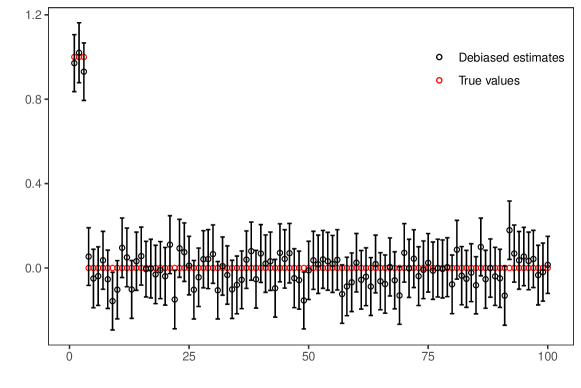
Figure 1: 95% confidence intervals for one realization of DP correction under the AR covariance structure with $\rho=0.5$ for the first $100$ regression parameters. The true parameters are denoted in red, and the debiased estimators are denoted in black.

To demonstrate the effectiveness of the proposed debiased procedure, we begin by displaying the estimated confidence intervals for the initial $100$ coordinates in one particular realization, as depicted in Figure 1. Notably, the estimated confidence intervals cover all of the signals, which are represented by the first three coordinates. The collective coverage for all the coordinates presented in the figure is approximately $95\%$. Further results can be found in Table 1 for the Toeplitz covariance design and in Table 2 for the equal correlation design.

Measure	Method	$\rho=0.0$	$\rho=0.2$	$\rho=0.4$	$\rho=0.6$
Avgcov	DB-Lasso	0.960	0.960	0.959	0.961
	DP naive	0.753	0.764	0.797	0.848
	DP correction	0.951	0.950	0.950	0.950
Avglength	DB-Lasso	0.190	0.195	0.219	0.261
	DP naive	0.179	0.187	0.210	0.265
	DP correction	0.304	0.309	0.324	0.361

Table 1: Average coverage and length of confidence intervals, for nominal coverage equal to 0.95, under Toeplitz covariance matrices.

Measure	Method	$\rho=0.1$	$\rho=0.3$	$\rho=0.5$	$\rho=0.7$
Avgcov	DB-Lasso	0.960	0.960	0.959	0.962
	DP naive	0.755	0.777	0.817	0.866
	DP correction	0.950	0.950	0.950	0.951
Avglength	DB-Lasso	0.191	0.204	0.234	0.282
	DP naive	0.182	0.196	0.228	0.291
	DP correction	0.306	0.314	0.335	0.381

Table 2: Average coverage and length of confidence intervals, for nominal coverage equal to 0.95, under blocked equal covariance matrices.

The numeric performance of our proposed debiased procedure exhibits remarkable similarity between the Toeplitz covariance design (Table 1) and the equal correlation design (Table 2). Notably, the coverage rates for DP naive fall significantly below the $95\%$ benchmark. It empirically proves our intuition that the additional correction is necessary for finite samples, as discussed in Section 4. In comparison, the DP correction method demonstrates significantly improved coverage compared to DP naive, albeit with wider confidence intervals. The corrected confidence intervals are approximately $30\%$ wider than those of DP naive. The interval length for DP correction is approximately $30\%$ greater than that of DB-Lasso, reflecting the efficiency loss stemming from privacy constraints. Overall, the proposed method exhibits coverage rates of approximately $95\%$ with only a marginal reduction in efficiency.

6.1.2 FDR control

Next, we proceed to assess the performance of the proposed algorithm for controlling the false discovery rate (FDR), as outlined in Section 5. To evaluate its effectiveness, we consider the Toeplitz covariance matrices (AR) defined as $\Sigma_{j,k}=\rho^{|j-k|}$ for $j,k\in\{1,\dots,p\}$. The active set, denoted as $S_{0}$, consists of $s_{0}=|S_{0}|=30$ randomly chosen covariates among all the available covariates. The nonzero regression coefficients $\beta_{j}$ for $j\in S_{0}$ are independently sampled from a normal distribution with mean 0 and variance $\xi$, where $\xi$ represents the signal strength. The errors in the linear model are assumed to follow a standard normal distribution, i.e., $e_{1},\dots,e_{n}\sim N(0,1)$. The sample size is set to $n=20,000$, and the number of covariates is $p=20,000$. For privacy preservation, we choose the privacy parameters $\epsilon=0.5$ and $\delta=1/n^{1.1}$. Moreover, we set the target FDR control level at $q=0.1$.

We compare our method with the non-private FDR control algorithm presented in Dai et al. (2022). The empirical FDR and power are reported, and all results are based on 100 independent simulations of the model with a fixed design and random regression coefficients (i.e., repeating the simulations 100 times with different errors in each linear model). Figure 2 presents the empirical FDR and power across various signal levels. Both the proposed differentially private FDR control procedure and the non-private procedure effectively control the empirical FDR at the predetermined level of $q=0.1$. The power of the proposed procedure exhibits a minor reduction compared to the non-private procedure due to privacy constraints. The numerical study demonstrates that, for reasonably large sample sizes, the proposed method can maintain FDR control with minimal sacrifice in power compared to the non-private approach.

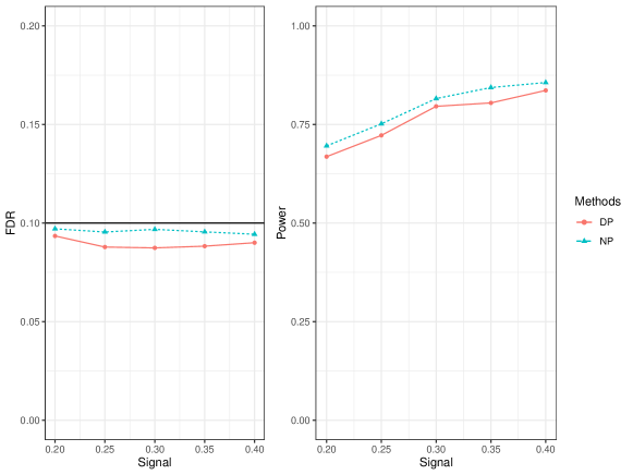
Figure 2: Empirical FDRs and powers of proposed methods with increasing signals $\xi$ for $\rho=0.2$ and $n=20,000$.

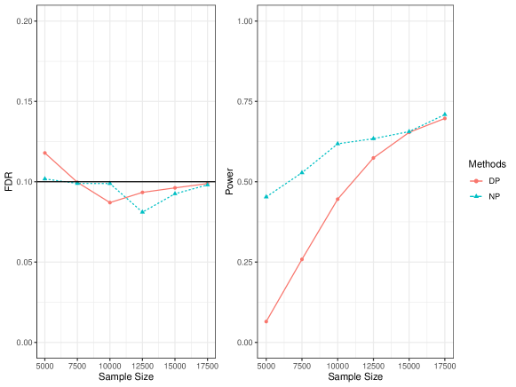
Figure 3: Empirical FDRs and powers of proposed methods with increasing sample sizes $n$ for $\rho=0.2$ and $\xi=0.2$.

Figure 3 presents the empirical FDR and power across increasing sample sizes. It is important to note that the proposed procedure may fail to control the empirical FDR when the sample size is very small. This is primarily due to the fact that in cases of small sample sizes, the initial step involving differentially private high-dimensional linear regression struggles to accurately identify all active features. Additionally, there may exist a nontrivial bias in the second step, which is the differentially private ordinary least square estimation. However, as the sample size increases, the proposed method successfully controls the empirical FDR at the predetermined level of $q=0.1$. Similarly, when dealing with small sample sizes, the power of the proposed procedure is notably lower than that of the non-private procedure due to the reduced estimation accuracy caused by privacy constraints. Nevertheless, as the sample size grows, both the differentially private algorithm and the non-private methods exhibit increased power, and the difference between them diminishes. This is a result of improved estimation accuracy in both the differentially private algorithm and the non-private algorithms. Overall, our numerical study demonstrates that for reasonably large sample sizes, the proposed method can effectively maintain FDR control with only a marginal reduction in power compared to the non-private approach.

6.2 Real Example: Parkinsons Telemonitoring

For real data applications, we demonstrate the performance of the proposed differentially private algorithms in analyzing the Parkinson’s Disease Progression data (Tsanas et al. (2009)). In clinical diagnosis, assessing the progression of Parkinson’s disease (PD) symptoms typically relies on the unified Parkinson’s disease rating scale (UPDRS), which necessitates the patient’s physical presence at the clinic and time-consuming physical evaluations conducted by trained medical professionals. Thus, monitoring symptoms is associated with high costs and logistical challenges for both patients and clinical staff. The target of this data set is to track UPDRS by noninvasive speech tests. However, it is crucial to protect the privacy of each patient’s data, as any unauthorized disclosure could lead to potential harm or trouble for the participants. By ensuring privacy protection, individuals are more likely to contribute their personal data, facilitating advancements in Parkinson’s disease research.

The data collection process involved the utilization of the Intel AHTD, a telemonitoring system designed for remote, internet-enabled measurement of various motor impairment symptoms associated with Parkinson’s disease (PD). The research was overseen by six U.S. medical centers, namely the Georgia Institute of Technology (seven subjects), National Institutes of Health (ten subjects), Oregon Health and Science University (fourteen subjects), Rush University Medical Center (eleven subjects), Southern Illinois University (six subjects), and the University of California Los Angeles (four subjects). A total of 52 individuals diagnosed with idiopathic PD were recruited. Following an initial screening process to eliminate flawed recordings (such as instances of patient coughing), a total of 5923 sustained phonations were subjected to analysis. In total, $16$ dysphonia measures were applied to the 5923 sustained phonations. Tsanas et al. (2009) proposed to use a linear model and didn’t consider privacy issues.

6.2.1 Debiased Inference

To evaluate the performance of our proposed differentially private inference algorithm 5 in high-dimensional settings, we add $5,000$ random features, which are generated independently identically from the standard normal distribution. Therefore, the dataset comprises a sample size of $n=5,923$ with covariates having a dimension of $p=5,016$, where the first $16$ of these covariates represent real features.

We consider the following three methods: the oracle method, the proposed differentially private algorithm, and the non-private debiased lasso (Van de Geer et al., 2014). The oracle method uses only the 16 real features, while the proposed algorithm and the debiased lasso utilize all 5,016 features. The privacy parameters are set as $\epsilon=0.5$ and $\delta=1/n^{1.1}$. Figure 4 displays the confidence intervals for the 16 real features obtained from the three methods. Overall, the private confidence intervals consistently cover the estimates obtained from the oracle method and the debiased lasso. In fact, the private confidence intervals exhibit substantial overlap with the confidence intervals from both the oracle method and the debiased lasso. However, due to the privacy costs, the width of the proposed confidence intervals is slightly larger than the confidence intervals from the debiased lasso.

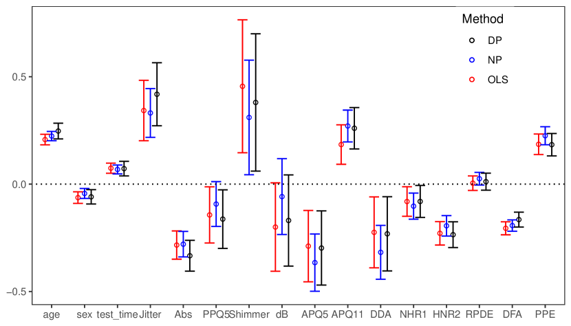
Figure 4: The $95\%$ confidence interval of OLS, nonprivate debiased lasso and proposed Algorithm 5 with finite sample correction.

6.2.2 FDR control

Next, we evaluate the performance of the private FDR control algorithm proposed in Section 5 on the Parkinson’s Disease Progression data. We add $100$ random features, which are generated independently and identically from $N(0,1)$. The proposed algorithm is compared with the nonprivate data splitting algorithm by Dai et al. (2022) and the knockoff by Barber and Candès (2015). The results are reported in Figure 5, where the target FDR is set to $0.1$ and $0.3$, respectively. The proposed method exhibits a notable count of discoveries within the real features while registering only a minimal number of false discoveries among the random features, compared to both knockoff and non-private data-splitting methods.

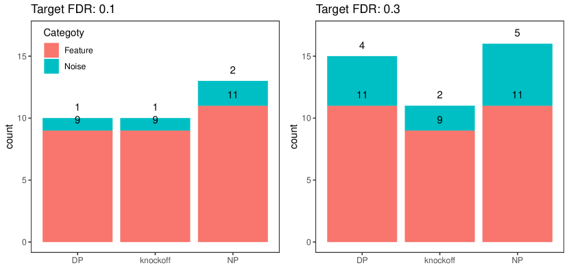
Figure 5: Numbers of the discovers.

feature	age	sex	test_time	Jitter	Abs	PPQ5	Shimmer	dB
knockoff	✓		✓	✓	✓
Non-Private	✓	✓	✓	✓	✓
DP-FDR	✓			✓	✓		✓
feature	APQ5	APQ11	DDA	NHR1	HNR2	RPDE	DFA	PPE
knockoff	✓	✓			✓		✓	✓
Non-Private		✓	✓	✓	✓		✓	✓
DP-FDR			✓		✓		✓	✓

Table 3: Selected Real Feature for Target $q=0.1$

We further report the selected features at the target FDR level of $q=0.1$ in Table 3. There is substantial overlap among the three methods, with several features being consistently selected. For instance, age, Jitter, Abs, HNR2, DFA, and PPE are all chosen by all three methods. For Parkinson’s disease (PD), which is the second most prevalent neurodegenerative disorder among the elderly, age is the most important impact factor. Numerous medical studies underscore the pivotal role of age as the single most significant factor associated with PD, as documented by Elbaz et al. (2002). Furthermore, Jitter and Abs are commonly employed to characterize cycle-to-cycle variability in fundamental frequency, while HNR (Harmonics-to-Noise Ratio) is a fundamental feature in speech processing techniques. Detrended Fluctuation Analysis (DFA) and Pitch Period Entropy (PPE) represent two recently proposed speech signal processing methods, both of which exhibit a strong correlation with PD-dysphonia, as highlighted in Little et al. (2008). In addition to these commonly selected features, the proposed method also identifies shimmer and DDA, which are frequently used to describe cycle-to-cycle variability in amplitude. Shimmer and DDA are also endorsed as relevant features in clinical studies by Tsanas et al. (2009). The features identified by our proposed method receive substantial clinical support, while with the privacy guarantee for the individual patients.

7 Discussion

This paper presents a comprehensive framework for performing differentially private analysis in high-dimensional linear models, encompassing estimation, inference, and false discovery rate (FDR) control. This framework is particularly valuable in scenarios where individual privacy in the dataset needs to be protected and can be readily applied across various disciplines. The numerical studies conducted in this work demonstrate that privacy protection can be achieved with only a minor loss in the accuracy of confidence intervals and multiple testing.

We briefly discuss several intriguing extensions. For example, the tools developed for DP estimation, debiased Lasso, and FDR control in this paper can all be extended to the generalized linear models. It would also be interesting to explore scenarios where a partial dataset, potentially following a different distribution, is publicly available and not bound by privacy constraints. Besides, the newly developed DP-BIC could be adapted for other tasks involving the selection of tuning parameters with privacy assurances. Those topics will be left for future research.

SUPPLEMENTARY MATERIAL

8 Proofs

8.1 The convergence rate in Algorithm 2

We now prove the differential privacy and convergence rate of $\hat{{\bm{\beta}}}$ in Algorithm 2.

8.1.1 Proof of Lemma 3.1

Proof of Lemma 3.1.

The $l_{\infty}$ sensitivity of of gradient in $t$th iteration
$-\eta_{0}/|S_{t}|\sum_{i\in S_{t}}(\Pi_{R}(\bm{x}_{i}^{\top}{\bm{\beta}}^{(t)})-\Pi_{R}(y_{i}))\bm{x}_{i}$ is

$$\sup_{(\bm{x}_{i},y_{i}),(\bm{x}_{i}^{\prime},y_{i}^{\prime})}\eta_{0}/|S_{t}|\cdot|(\Pi_{R}(\bm{x}_{i}^{\top}{\bm{\beta}}^{(t)})-\Pi_{R}(y_{i}))\bm{x}_{i}-(\Pi_{R}(\bm{x}_{i}^{\prime\top}{\bm{\beta}}^{(t)})-\Pi_{R}(y_{i}^{\prime}))\bm{x}_{i}^{\prime}|\leq\eta_{0}T/n\cdot 2(R+R)c_{x}.$$

By advanced composition theorem, outputting the gradient is $(\epsilon/\{T(K+2)\},\delta/\{T(K+1)\})$-differentially private. Thus, furthermore, by composition theorem, for $0\leq k\leq K$, output $\hat{{\bm{\beta}}}(k)$ is $(\epsilon/(K+2),\delta/(K+1))$-differential privacy. By composition theorem, returning all $\{\hat{{\bm{\beta}}}(k)\}_{k=0}^{K}$ is $(\epsilon(K+1)/(K+2),\delta)$-differential privacy.

Then, we consider the sensitivity of BIC loss. Notice that

$$\sup_{(\bm{x}_{i},y_{i}),(\bm{x}_{i}^{\prime},y_{i}^{\prime})}|(\Pi_{R}(\bm{x}_{i}^{\top}{\bm{\beta}}(k))-\Pi_{R}(y_{i}))^{2}-(\Pi_{R}(\bm{x}_{i}^{\prime\top}{\bm{\beta}}(k))-\Pi_{R}(y_{i}^{\prime}))^{2}|\leq 2(R+R)^{2},$$

for every $0\leq k\leq K$. The BIC selection procedure returns the noisy minimum. By Dwork and Roth (2014), the BIC selection procedure is $(\epsilon/(K+2),0)$-differential privacy. Finally, by composition theorem, the Algorithm 2 is $(\epsilon,\delta)$-differential privacy. ∎

8.1.2 Proof of Theorem 3.1

Proof of Theorem 3.1.

Let $\hat{k}$ be the selected number corresponds to $\hat{{\bm{\beta}}}$ and $k^{*}$ be such that $2^{k^{*}-1}<\rho L^{4}s\leq 2^{k^{*}}$. Note that $k^{*}$ is uniquely defined by $s$ and $(\rho,L)$. Define events

$$E_{0}=\big{\{}\inf_{\|{\mathbf{u}}\|_{0}=o(n),\|{\mathbf{u}}\|_{2}=1}{{\mathbf{u}}}^{T}\widehat{\bm{\Sigma}}{{\mathbf{u}}}\geq c\|{\mathbf{u}}\|_{2}^{2}\big{\}},$$

where $\widehat{\bm{\Sigma}}={\bm{X}}^{\top}{\bm{X}}/n$, and

$$E_{1}=\big{\{}\|\hat{{\bm{\beta}}}(k)-{\bm{\beta}}\|_{2}\leq c_{2}\frac{2^{k}\log p\log n}{n}+c_{3}\frac{2^{2k}\log(p)^{2}\log(1/\delta)\log^{7}n}{n^{2}\epsilon^{2}}\text{ for }2^{k}\geq\rho L^{4}s\big{\}}.$$

By Theorem 4.4 in Cai et al. (2021) and replacing $T$ in Cai et al. (2021) by $KT$, the event $E_{1}$ happens with probability at least $1-\exp(-c_{1}\log n)$.

By the oracle inequality of the BIC criterion,

$$\|\bm{y}-{\bm{X}}\hat{{\bm{\beta}}}\|_{2}^{2}+c_{0}f(n,\hat{k})\leq\|\bm{y}-{\bm{X}}\hat{{\bm{\beta}}}(k^{*})\|_{2}^{2}+c_{0}f(n,k^{*})+\epsilon_{privacy},$$

where $f(n,k)=2^{k}\log p\log n+\frac{2^{2k}\log(p)^{2}\log(1/\delta)\log^{7}n}{n\epsilon^{2}}$ and $\epsilon_{privacy}$ is the additional term equals to $\sup_{k}|z_{k}|$. It implies that

$$\|{\bm{X}}(\hat{{\bm{\beta}}}-\hat{{\bm{\beta}}}(k^{*}))\|_{2}^{2}\leq 2|\langle{\bm{X}}(\hat{{\bm{\beta}}}-\hat{{\bm{\beta}}}(k^{*})),\bm{y}-{\bm{X}}\hat{{\bm{\beta}}}(k^{*})\rangle|+c_{0}\{f(n,k^{*})-f(n,\hat{k})\}+\epsilon_{privacy}.$$

Let $\widehat{U}=supp(\hat{{\bm{\beta}}}-\hat{{\bm{\beta}}}(k^{*}))$. Note that

$$|\widehat{U}|=\sqrt{n}/\log^{2}p+s=o(n).$$

Hence, by the first statement in $E_{0}$, we have

$$c\|\hat{{\bm{\beta}}}-\hat{{\bm{\beta}}}(k^{*})\|_{2}^{2}\leq\frac{1}{n}\|{\bm{X}}(\hat{{\bm{\beta}}}-\hat{{\bm{\beta}}}(k^{*}))\|_{2}^{2}$$

$$\leq \frac{2}{n}|\langle{\bm{X}}(\hat{{\bm{\beta}}}-\hat{{\bm{\beta}}}(k^{*})),{\bm{X}}(\hat{{\bm{\beta}}}(k^{*})-{\bm{\beta}})\rangle|+\frac{2}{n}|\langle{\bm{X}}(\hat{{\bm{\beta}}}-\hat{{\bm{\beta}}}(k^{*})),\bm{y}-{\bm{X}}{\bm{\beta}}\rangle|$$

$$+c_{0}\{f(n,k^{*})-f(n,\hat{k})\}/n+\epsilon_{privacy}/n$$

$$\leq \frac{2}{n}\|{\bm{X}}(\hat{{\bm{\beta}}}-\hat{{\bm{\beta}}}(k^{*}))\|_{2}\|{\bm{X}}(\hat{{\bm{\beta}}}(k^{*})-{\bm{\beta}})\|_{2}+2\|\hat{{\bm{\beta}}}-\hat{{\bm{\beta}}}(k^{*})\|_{1}\|\frac{1}{n}{\bm{X}}\epsilon\|_{\infty}$$

$$+c_{0}\{f(n,k^{*})-f(n,\hat{k})\}/n+\epsilon_{privacy}/n$$

$$\leq C\|\hat{{\bm{\beta}}}-\hat{{\bm{\beta}}}(k^{*})\|_{2}\|\hat{{\bm{\beta}}}(k^{*})-{\bm{\beta}}\|_{2}+{C\|\hat{{\bm{\beta}}}-\hat{{\bm{\beta}}}(k^{*})\|_{1}\sqrt{\frac{\log p}{n}}}+c_{0}\{f(n,k^{*})-f(n,\hat{k})\}/n$$

$$+\epsilon_{privacy}/n$$

with high probability, where we use Hölder’s inequality and concentration inequality. We first consider the case where $\hat{k}<k^{*}$. Then, by the Hölder’s inequality,

$$\begin{split}c\|\hat{{\bm{\beta}}}-\hat{{\bm{\beta}}}(k^{*})\|_{2}^{2}\leq&C\|\hat{{\bm{\beta}}}-\hat{{\bm{\beta}}}(k^{*})\|_{2}\|\hat{{\bm{\beta}}}(k^{*})-{\bm{\beta}}\|_{2}+C\|\hat{{\bm{\beta}}}-\hat{{\bm{\beta}}}(k^{*})\|_{2}\sqrt{\frac{(2^{\hat{k}}+2^{k^{*}})\log p}{n}}\\ &+c_{0}\{f(n,k^{*})-f(n,\hat{k})\}/n+\epsilon_{privacy}/n\\ \leq&2C\|\hat{{\bm{\beta}}}-\hat{{\bm{\beta}}}(k^{*})\|_{2}\|\hat{{\bm{\beta}}}(k^{*})-{\bm{\beta}}\|_{2}+c_{0}\{f(n,k^{*})-f(n,\hat{k})\}/n+\epsilon_{privacy}/n\end{split}$$

By the assumption that $\hat{k}<k^{*}$, we have $c_{0}\{f(n,k^{*})-f(n,\hat{k})\}+\epsilon_{privacy}>0$ for $c_{0}>0$. Thus, the solution of quadratic inequality exists and satisfies,

$$\begin{split}&\|\hat{{\bm{\beta}}}-\hat{{\bm{\beta}}}(k^{*})\|_{2}\\ &\leq\frac{C\|\hat{{\bm{\beta}}}(k^{*})-{\bm{\beta}}\|_{2}+\sqrt{C^{2}\|\hat{{\bm{\beta}}}(k^{*})-{\bm{\beta}}\|_{2}^{2}+c\{c_{0}\{f(n,k^{*})-f(n,\hat{k})\}/n+\epsilon_{privacy}/n\}}}{c}\\ &\leq C^{\prime}\|\hat{{\bm{\beta}}}(k^{*})-{\bm{\beta}}\|_{2},\end{split}$$

for a constant $C^{\prime}$. Then, we consider the case where $\hat{k}\geq k^{*}$. By Hölder’s inequality and triangle inequality, we have

$$c\|\hat{{\bm{\beta}}}-\hat{{\bm{\beta}}}(k^{*})\|_{2}^{2}\leq C\|\hat{{\bm{\beta}}}-\hat{{\bm{\beta}}}(k^{*})\|_{2}\|\hat{{\bm{\beta}}}(k^{*})-{\bm{\beta}}\|_{2}+C\|\hat{{\bm{\beta}}}-\hat{{\bm{\beta}}}(k^{*})\|_{1}\sqrt{\frac{\log p}{n}}$$

$$+c_{0}\{f(n,k^{*})-f(n,\hat{k})\}/n+\epsilon_{privacy}/n$$

$$\leq C\|\hat{{\bm{\beta}}}(k^{*})-{\bm{\beta}}\|_{2}^{2}+C\|\hat{{\bm{\beta}}}-{\bm{\beta}}\|_{2}^{2}+C\|\hat{{\bm{\beta}}}-{\bm{\beta}}\|_{1}\sqrt{\frac{\log p}{n}}$$

$$+C\|{\bm{\beta}}-\hat{{\bm{\beta}}}(k^{*})\|_{1}\sqrt{\frac{\log p}{n}}+c_{0}\{f(n,k^{*})-f(n,\hat{k})\}/n+\epsilon_{privacy}/n$$

$$\leq 2C\|\hat{{\bm{\beta}}}(k^{*})-{\bm{\beta}}\|_{2}^{2}+2C\bigg{\{}c_{2}\frac{2^{\hat{k}}\log p\log n}{n}+c_{3}\frac{2^{2\hat{k}}\log p\log^{7}n\log(1/\delta)}{n^{2}\epsilon^{2}}\bigg{\}}$$

$$+c_{0}\{f(n,k^{*})-f(n,\hat{k})\}/n+\epsilon_{privacy}/n.$$

For $c_{0}>2C$, we have

$$c\|\hat{{\bm{\beta}}}-\hat{{\bm{\beta}}}(k^{*})\|_{2}^{2}\leq(2C+c_{0})\|\hat{{\bm{\beta}}}(k^{*})-{\bm{\beta}}\|_{2}^{2}+\epsilon_{privacy}/n.$$

The conclusion holds. ∎

8.2 Proofs of Statistical Inference

Given a pre-specified sparsity level $s_{j}$, the differentially private estimation of $\bm{w}_{j}$ algorithm is presented in Algorithm 7.

Input : dataset $\{(\bm{x}_{i},y_{i})\}_{i\in[n]}$, step size $\eta^{0}$, privacy parameters $\varepsilon,\delta$, noise scale $B$, number of iterations $T$, truncation level $R$, feasibility parameter $C$, sparsity $s^{*}$, initial value $\bm{w}^{0}$.

1 Random split data into $T$ parts of roughly equal sizes: $[n]=\mathcal{S}_{0}\cup\dots\cup\mathcal{S}_{T-1}$ and $\mathcal{S}_{i}\cap\mathcal{S}_{j}=\emptyset$ for $i\neq j$;

2for $t$ in $0$ to $T-1$ do

3       Compute $\bm{w}^{(t+0.5)}=\bm{w}^{(t)}-\eta^{0}(\bm{e}_{j}-\sum_{i\in\mathcal{S}_{t}}\bm{x}_{i}\Pi_{R}(\bm{x}_{i}^{\top}\bm{w}^{(t)})/|\mathcal{S}_{t}|)$;

4       $\bm{w}^{(t+1)}=\Pi_{C}(\text{NoisyIHT}(\bm{w}^{(t+0.5)},s^{*},\varepsilon/T,\delta/T,\eta^{0}B/n))$.

5 end for

6

Output : $\bm{w}_{j}^{(T)}$.

Algorithm 7 Differentially Private Estimation of $\bm{w}_{j}$ given sparsity

Theoretical properties of Algorithm 7 are outlined in Lemma 8.1. The proof follows the similar arguments of Theorem 4.4 in Cai et al. (2021).

Lemma 8.1.

Suppose conditions 3.1, 3.2 and 4.1 hold, and let $B=2Rc_{x}$, $C>L$ and $R=2L\log(n)$. There exists a constant $\rho$ such that, if $s^{*}=\rho L^{4}s_{j}$, $\eta^{0}=1/6L$, $T=\rho L^{2}\log(8L^{3}n)$, $s\log p=o(n)$ and $s\log p\log(1/\delta)\log^{3}n/\epsilon=o(n)$. Then with probability at least $1-\exp(-c_{1}\log n)$, there exist constants $c_{2}$ and $c_{3}$, such that

$$\|\bm{w}_{j}^{(T)}-\bm{w}_{j}\|_{2}^{2}\leq c_{1}\frac{s^{*}\log p\log n}{n}+c_{2}\frac{s^{*2}\log^{2}p\log(1/\delta)\log^{4}n}{n^{2}\epsilon^{2}}.$$

8.2.1 Proofs of Lemma 8.1

Proofs of Lemma 8.1.

Let $S_{0}=\text{supp}(\bm{w}_{j})$ be the support of true parameter $\bm{w}_{j}$ and for any subset $S$ satisfies $S_{0}\subset S$ and $|S|\leq cs_{j}$. The oracle estimator $\hat{\bm{w}}_{j}$ is defined by

$$\hat{\bm{w}}_{j}=\operatorname*{arg\,min}_{\bm{w}\in\mathbb{R}^{p},\text{supp}(\bm{w})\in S}{\mathcal{L}}_{n}(\bm{w}):=\frac{1}{2}\bm{w}^{\top}\hat{\Sigma}\bm{w}-\bm{w}^{T}\bm{e}_{j}.$$

We first study the statistical property of $\hat{\bm{w}}_{j}$. An equivalent formulation of $\hat{\bm{w}}_{j}$ is $\hat{\bm{w}}_{j,S}=\operatorname*{arg\,min}_{\bm{w}\in\mathbb{R}^{|}S|}\frac{1}{2}\bm{w}^{\top}\hat{\Sigma}_{SS}\bm{w}-\bm{w}^{\top}\bm{e}_{j,S}$, where $\hat{\bm{w}}_{j,S}$ is a sub-vector of $\hat{\bm{w}}_{j}$ and $\hat{\Sigma}_{SS}$ is a sub-matrix of $\hat{\Sigma}$. Notice that $j\in S$, the sub-vector $\bm{e}_{j,S}$ is a unit vector. Then, we have an analytic solution $\hat{\bm{w}}_{j,S}=\hat{\Sigma}_{SS}^{-1}\bm{e}_{j,S}$. Then,

$$\|\hat{\bm{w}}_{j}-\bm{w}_{j}\|_{2}=\|\hat{\bm{w}}_{j,S}-\bm{w}_{j,S}\|_{2}=\|(\hat{\Sigma}_{SS}^{-1}-\Sigma_{SS}^{-1})\bm{e}_{j,S}\|_{2}\leq\|\hat{\Sigma}_{SS}^{-1}-\Sigma_{SS}^{-1}\|_{2}.$$

By Corollary 10.1 in Tan et al. (2020), we have for any constant $C^{\prime}$, there exists some constant $C>0$, such that

$$\|\hat{\bm{w}}_{j}-\bm{w}_{j}\|_{2}^{2}\leq\frac{C}{n}s_{j}\log(ep/s_{j}),$$

with probability at least $1-\exp\{-C^{\prime}s_{j}\log(ep/s_{j})\}$.

Then, the ${\mathcal{L}}_{n}(\bm{w})$ satisfy $\langle\nabla{\mathcal{L}}_{n}(\bm{w}_{1})-\nabla{\mathcal{L}}_{n}(\bm{w}_{2}),\bm{w}_{1}-\bm{w}_{2}\rangle=(\bm{w}_{1}-\bm{w}_{2})^{\top}\hat{\Sigma}(\bm{w}_{1}-\bm{w}_{2})$. Thus, we have

$$\alpha\|\bm{w}_{1}-\bm{w}_{2}\|_{2}^{2}\leq\langle\nabla{\mathcal{L}}_{n}(\bm{w}_{1})-\nabla{\mathcal{L}}_{n}(\bm{w}_{2}),\bm{w}_{1}-\bm{w}_{2}\rangle\leq\gamma\|\bm{w}_{1}-\bm{w}_{2}\|_{2}^{2},$$

for $\bm{w}_{1},\bm{w}_{2}\in\mathbb{R}^{p}$ satisfying $\max\{|\text{supp}(\bm{w}_{1})|,|\text{supp}(\bm{w}_{2})|\}\leq cs$. Then, we have

$$\begin{split}{\mathcal{L}}_{n}(\hat{\bm{w}}_{j}^{(t+1)})-{\mathcal{L}}_{n}(\hat{\bm{w}}_{j}^{(t)})&=\frac{1}{2}\hat{\bm{w}}_{j}^{(t+1)\top}\hat{\Sigma}\hat{\bm{w}}_{j}^{(t+1)}-\frac{1}{2}\hat{\bm{w}}_{j}^{(t)\top}\hat{\Sigma}\hat{\bm{w}}_{j}^{(t)}-(\hat{\bm{w}}_{j}^{(t+1)}-\hat{\bm{w}}_{j}^{(t)})^{\top}\bm{e}_{j}\\ &=\langle\hat{\bm{w}}_{j}^{(t+1)}-\hat{\bm{w}}_{j}^{(t)},\hat{\bm{w}}_{j}^{(t)\top}\hat{\Sigma}-\bm{e}_{j}\rangle+\frac{1}{2}(\hat{\bm{w}}_{j}^{(t+1)}-\hat{\bm{w}}_{j}^{(t)})^{\top}\hat{\Sigma}(\hat{\bm{w}}_{j}^{(t+1)}-\hat{\bm{w}}_{j}^{(t)})\\ &\leq\langle\hat{\bm{w}}_{j}^{(t+1)}-\hat{\bm{w}}_{j}^{(t)},\bm{g}^{t}\rangle+\frac{\gamma}{2}\|\hat{\bm{w}}_{j}^{(t+1)}-\hat{\bm{w}}_{j}^{(t)}\|_{2}^{2},\end{split}$$

where $\bm{g}_{t}=\hat{\bm{w}}_{j}^{(t)\top}\hat{\Sigma}-\bm{e}_{j}$ is the gradient of ${\mathcal{L}}_{n}(\bm{w})$ evaluated at $\hat{\bm{w}}_{j}^{t}$. Let $S^{t}=\text{supp}(\hat{\bm{w}}_{j}^{(t)})$, $S^{t+1}=\text{supp}(\hat{\bm{w}}_{j}^{(t+1)})$ and $I^{t}=S^{t+1}\cup S^{t}\cup S$. Let $\bm{n}_{1},\bm{n}_{2},\dots$ be the noise vectors added to $\hat{\bm{w}}_{j}-\eta\nabla{\mathcal{L}}_{n}(\hat{\bm{w}}_{j}^{(t)})$ after the peeling mechanism and $\bm{N}=4\sum_{i\in[s]}\|\bm{n}_{i}\|^{2}_{\infty}$. Then, we have the decomposition,

$$\begin{split}&\langle\hat{\bm{w}}_{j}^{(t+1)}-\hat{\bm{w}}_{j}^{(t)},\bm{g}^{t}\rangle+\frac{\gamma}{2}\|\hat{\bm{w}}_{j}^{(t+1)}-\hat{\bm{w}}_{j}^{(t)}\|_{2}^{2}\\ =&\frac{\gamma}{2}\|\hat{\bm{w}}_{j,I^{t}}^{(t+1)}-\hat{\bm{w}}_{j,I^{t}}^{(t)}+\frac{\eta}{\gamma}\bm{g}^{t}_{I^{t}}\|_{2}^{2}-\frac{\eta^{2}}{2\gamma}\|\bm{g}^{t}_{I^{t}}\|_{2}^{2}+(1-\eta)\langle\hat{\bm{w}}_{j}^{(t+1)}-\hat{\bm{w}}_{j}^{(t)},\bm{g}^{t}\rangle.\end{split}$$

We first consider the first two terms. Let the subset $R=S^{t}/S^{t+1}$, then $|I^{t}/(S^{t}\cup S)|=|S^{t}/S^{t+1}|$. Then, by the fact $\hat{\bm{w}}^{(t)}_{j,I^{t}/(S^{t}\cup S)}=\bm{0}$ and the selection criterion, we have for every $c>1$

$$\frac{\eta^{2}}{\gamma^{2}}\|\bm{g}^{t}_{I^{t}/(S^{t}\cup S)}\|_{2}^{2}=\|\hat{\bm{w}}_{j,I^{t}/(S^{t}\cup S)}^{(t)}-\frac{\eta^{2}}{\gamma^{2}}\bm{g}^{t}_{I^{t}/(S^{t}\cup S)}\|_{2}^{2}\geq(1-1/c)\|\hat{\bm{w}}_{j,R}^{(t)}-\frac{\eta^{2}}{\gamma^{2}}\bm{g}^{t}_{R}\|_{2}^{2}-c\bm{N}.$$

Then, we have

$$\begin{split}&\frac{\gamma}{2}\|\hat{\bm{w}}_{j,I^{t}}^{(t+1)}-\hat{\bm{w}}_{j,I^{t}}^{(t)}+\frac{\eta}{\gamma}\bm{g}^{t}_{I^{t}}\|_{2}^{2}-\frac{\eta^{2}}{2\gamma}\|\bm{g}^{t}_{I^{t}/(S^{t}\cup S)}\|_{2}^{2}\\ \leq&\gamma\|\bm{n}_{S^{t+1}}\|_{2}^{2}+\gamma\|\tilde{\bm{w}}_{j,I^{t}}^{(t+1)}-\hat{\bm{w}}_{j,I^{t}}^{(t)}+\frac{\eta}{\gamma}\bm{g}^{t}_{I^{t}}\|_{2}^{2}-\frac{\gamma}{2}(1-1/c)\|\hat{\bm{w}}_{j,R}^{(t)}-\frac{\eta^{2}}{\gamma^{2}}\bm{g}^{t}_{R}\|_{2}^{2}+\frac{c\gamma}{2}\bm{N}\\ =&\gamma\|\tilde{\bm{w}}_{j,I^{t}}^{(t+1)}-\hat{\bm{w}}_{j,I^{t}}^{(t)}+\frac{\eta}{\gamma}\bm{g}^{t}_{I^{t}}\|_{2}^{2}-\gamma\|\tilde{\bm{w}}_{j,R}^{(t+1)}-\hat{\bm{w}}_{j,R}^{(t)}+\frac{\eta}{\gamma}\bm{g}^{t}_{R}\|_{2}^{2}+\frac{\gamma}{2}(1+1/c)\|\hat{\bm{w}}_{j,R}^{(t)}-\frac{\eta^{2}}{\gamma^{2}}\bm{g}^{t}_{R}\|_{2}^{2}\\ &+\gamma\|\bm{n}_{S^{t+1}}\|_{2}^{2}+\frac{c\gamma}{2}\bm{N}\\ \leq&\gamma\|\tilde{\bm{w}}_{j,I^{t}/R}^{(t+1)}-\hat{\bm{w}}_{j,I^{t}/R}^{(t)}+\frac{\eta}{\gamma}\bm{g}^{t}_{I^{t}/R}\|_{2}^{2}+\frac{\eta^{2}}{2\gamma}\frac{c+1}{c-1}\|\bm{g}^{t}_{I^{t}/(S^{t}\cup S)}\|_{2}^{2}+\gamma\|\bm{n}_{S^{t+1}}\|_{2}^{2}+\frac{c\gamma}{2}(\frac{c+1}{c-1}c+1)\bm{N},\end{split}$$

where we use $(a+b)^{2}\leq 2a^{2}+2b^{2}$ in the first inequality. By Lemma A.3. in Cai et al. (2021), we have

$$\|\tilde{\bm{w}}_{j,I^{t}/R}^{(t+1)}-\hat{\bm{w}}_{j,I^{t}/R}^{(t)}+\frac{\eta}{\gamma}\bm{g}^{t}_{I^{t}/R}\|_{2}^{2}\leq\frac{3}{2}\frac{|I^{t}/R|-s}{|I^{t}/R|-s^{*}}\|\hat{\bm{w}}_{j,I^{t}}-\hat{\bm{w}}_{j,I^{t}}^{(t)}+\frac{\eta}{\gamma}\bm{g}^{t}_{I^{t}}\|_{2}^{2}+3\bm{N}.$$

Thus,

$$\begin{split}&\frac{\gamma}{2}\|\hat{\bm{w}}_{j,I^{t}}^{(t+1)}-\hat{\bm{w}}_{j,I^{t}}^{(t)}+\frac{\eta}{\gamma}\bm{g}^{t}_{I^{t}}\|_{2}^{2}-\frac{\eta^{2}}{2\gamma}\|\bm{g}^{t}_{I^{t}/(S^{t}\cup S)}\|_{2}^{2}\\ \leq&\gamma\frac{3}{2}\frac{|I^{t}/R|-s_{j}}{|I^{t}/R|-s^{*}}\|\hat{\bm{w}}_{j,I^{t}}-\hat{\bm{w}}_{j,I^{t}}^{(t)}+\frac{\eta}{\gamma}\bm{g}^{t}_{I^{t}}\|_{2}^{2}+3\bm{\gamma}N+\frac{\eta^{2}}{2\gamma}\frac{c+1}{c-1}\|\bm{g}^{t}_{I^{t}/(S^{t}\cup S)}\|_{2}^{2}\\ &+\gamma\|\bm{n}_{S^{t+1}}\|_{2}^{2}+\frac{c\gamma}{2}(\frac{c+1}{c-1}c+1)\bm{N}\\ =&\frac{3s^{*}}{s_{j}+s^{*}}(2\eta\langle\hat{\bm{w}}_{j}-\hat{\bm{w}}_{j}^{(t)},\bm{g}^{t}\rangle+\gamma\|\hat{\bm{w}}_{j}-\hat{\bm{w}}_{j}^{(t)}\|_{2}^{2}+\frac{\eta^{2}}{\gamma}\|\bm{g}^{t}_{I^{t}}\|_{2}^{2})+\frac{\eta^{2}}{2\gamma}\frac{c+1}{c-1}\|\bm{g}^{t}_{I^{t}/(S^{t}\cup S)}\|_{2}^{2}\\ &+\gamma\|\bm{n}_{S^{t+1}}\|_{2}^{2}+\frac{c\gamma}{2}(\frac{c+1}{c-1}c+1+6/c)\bm{N}\\ \leq&\frac{3s^{*}}{s_{j}+s^{*}}[2\eta\{{\mathcal{L}}_{n}(\hat{\bm{w}}_{j})-{\mathcal{L}}_{n}(\hat{\bm{w}}_{j}^{(t)})\}+(\gamma-2\eta\alpha)\|\hat{\bm{w}}_{j}-\hat{\bm{w}}_{j}^{(t)}\|_{2}^{2}+\frac{\eta^{2}}{\gamma}\|\bm{g}^{t}_{I^{t}}\|_{2}^{2}]\\ &+\frac{\eta^{2}}{2\gamma}\frac{c+1}{c-1}\|\bm{g}^{t}_{I^{t}/(S^{t}\cup S)}\|_{2}^{2}+\gamma\|\bm{n}_{S^{t+1}}\|_{2}^{2}+\frac{c\gamma}{2}(\frac{c+1}{c-1}c+1+6/c)\bm{N},\end{split}$$

where in the first inequality, we use the assumption $s_{j}>s^{*}$.

Then, we consider the second term, which has the decomposition

$$\begin{split}\langle\hat{\bm{w}}_{j}^{(t+1)}-\hat{\bm{w}}_{j}^{(t)},\bm{g}^{t}\rangle&=\langle\tilde{\bm{w}}_{j,S^{t+1}}^{(t+1)}-\hat{\bm{w}}_{j,S^{t+1}}^{(t)},\bm{g}^{t}_{S^{t+1}}\rangle+\langle\bm{n}_{S^{t+1}},\bm{g}^{t}_{S^{t+1}}\rangle-\langle\hat{\bm{w}}_{j,S^{t}/S^{t+1}}^{(t)},\bm{g}_{S^{t}/S^{t+1}}^{t}\rangle\\ &\leq-\frac{\eta}{\gamma}\|\bm{g}^{t}_{S^{t}}\|_{2}^{2}+c\|\bm{n}_{S^{t+1}}\|_{2}^{2}+(1/4c)\|\bm{g}^{t}_{S^{t+1}}\|^{2}_{2}-\langle\hat{\bm{w}}_{j,S^{t}/S^{t+1}}^{(t)},\bm{g}_{S^{t}/S^{t+1}}^{t}\rangle,\end{split}$$

where we use the fact that $ab\leq a^{2}/2+b^{2}/2$. The last term satisfies

$$-\langle\hat{\bm{w}}_{j,S^{t}/S^{t+1}}^{(t)},\bm{g}_{S^{t}/S^{t+1}}^{t}\rangle\leq\frac{\gamma}{2\eta}\{\|\hat{\bm{w}}_{j,S^{t}/S^{t+1}}^{(t)}-\frac{\eta}{\gamma}\bm{g}_{S^{t}/S^{t+1}}^{t}\|_{2}^{2}-(\frac{\eta}{\gamma})^{2}\|\bm{g}_{S^{t}/S^{t+1}}^{t}\|_{2}^{2}\}.$$

By the selection property, we have

$$\begin{split}-\langle\hat{\bm{w}}_{j,S^{t}/S^{t+1}}^{(t)},\bm{g}_{S^{t}/S^{t+1}}^{t}\rangle&\leq\frac{\gamma}{2\eta}\{(1+1/c)\|\tilde{\bm{w}}_{j,S^{t+1}/S^{t}}^{(t)}\|_{2}^{2}+(1+c)\bm{N}\}-\frac{\eta}{2\gamma}\|\bm{g}_{S^{t}/S^{t+1}}^{t}\|_{2}^{2}\\ &=\frac{\eta}{2\gamma}\{(1+1/c)\|\bm{g}_{S^{t+1}/S^{t}}^{t}\|_{2}^{2}+(1+c)\bm{N}\}-\frac{\eta}{2\gamma}\|\bm{g}_{S^{t}/S^{t+1}}^{t}\|_{2}^{2}\end{split}$$

By combining the results together, we have

$$\begin{split}\langle\hat{\bm{w}}_{j}^{(t+1)}-\hat{\bm{w}}_{j}^{(t)},\bm{g}^{t}\rangle\leq&-\frac{\eta}{\gamma}\|\bm{g}^{t}_{S^{t+1}}\|_{2}^{2}+c\|\bm{n}_{S^{t+1}}\|_{2}^{2}+(1/4c)\|\bm{g}^{t}_{S^{t+1}}\|^{2}_{2}\\ &+\frac{\gamma}{2\eta}\{(1+1/c)\|\bm{g}_{S^{t+1}/S^{t}}^{t}\|_{2}^{2}+(1+c)\bm{N}\}-\frac{\eta}{2\gamma}\|\bm{g}_{S^{t}/S^{t+1}}^{t}\|_{2}^{2}\\ \leq&\frac{\eta}{2\gamma}\|\bm{g}_{S^{t+1}/S^{t}}^{t}\|_{2}^{2}-\frac{\eta}{2\gamma}\|\bm{g}_{S^{t}/S^{t+1}}^{t}\|_{2}^{2}-\frac{\eta}{\gamma}\|\bm{g}^{t}_{S^{t+1}}\|_{2}^{2}\\ &+(1/c)(4+\frac{\eta}{2\gamma})\|\bm{g}^{t}_{S^{t+1}}\|^{2}_{2}+c\|\bm{n}_{S^{t+1}}\|_{2}^{2}+(1+c)\frac{\gamma}{2\eta}\bm{N}\\ \leq&-\frac{\eta}{2\gamma}\|\bm{g}_{S^{t}\cup S^{t+1}}^{t}\|_{2}^{2}+(1/c)(4+\frac{\eta}{2\gamma})\|\bm{g}^{t}_{S^{t+1}}\|^{2}_{2}+c\|\bm{n}_{S^{t+1}}\|_{2}^{2}+(1+c)\frac{\gamma}{2\eta}\bm{N}.\end{split}$$

Combining all results together, we have

$$\begin{split}&{\mathcal{L}}_{n}(\hat{\bm{w}}_{j}^{(t+1)})-{\mathcal{L}}_{n}(\hat{\bm{w}}_{j}^{(t)})\\ \leq&\frac{\gamma}{2}\|\hat{\bm{w}}_{j,I^{t}}^{(t+1)}-\hat{\bm{w}}_{j,I^{t}}^{(t)}+\frac{\eta}{\gamma}\bm{g}^{t}_{I^{t}}\|_{2}^{2}-\frac{\eta^{2}}{2\gamma}\|\bm{g}^{t}_{I^{t}}\|_{2}^{2}-\frac{\eta(1-\eta)}{2\gamma}\|\bm{g}_{S^{t}\cup S^{t+1}}^{t}\|_{2}^{2}\\ &+(1-\eta)(1/c)(4+\frac{\eta}{2\gamma})\|\bm{g}^{t}_{S^{t+1}}\|^{2}_{2}+c(1-\eta)\|\bm{n}_{S^{t+1}}\|_{2}^{2}+(1-\eta)(1+c)\frac{\gamma}{2\eta}\bm{N}\\ \leq&\frac{\gamma}{2}\|\hat{\bm{w}}_{j,I^{t}}^{(t+1)}-\hat{\bm{w}}_{j,I^{t}}^{(t)}+\frac{\eta}{\gamma}\bm{g}^{t}_{I^{t}}\|_{2}^{2}-\frac{\eta^{2}}{2\gamma}\|\bm{g}^{t}_{I^{t}/(S^{t}\cup S)}\|_{2}^{2}-\frac{\eta^{2}}{2\gamma}\|\bm{g}^{t}_{S^{t}\cup S}\|_{2}^{2}\\ &-\frac{\eta(1-\eta)}{2\gamma}\|\bm{g}_{S^{t+1}/(S^{t}\cup S)}^{t}\|_{2}^{2}+(1-\eta)(1/c)(4+\frac{\eta}{2\gamma})\|\bm{g}^{t}_{S^{t+1}}\|^{2}_{2}\\ &+c(1-\eta)\|\bm{n}_{S^{t+1}}\|_{2}^{2}+(1-\eta)(1+c)\frac{\gamma}{2\eta}\bm{N}\\ \leq&\frac{3s^{*}}{s_{j}+s^{*}}[2\eta\{{\mathcal{L}}_{n}(\hat{\bm{w}}_{j})-{\mathcal{L}}_{n}(\hat{\bm{w}}_{j}^{(t)})\}+(\gamma-2\eta\alpha)\|\hat{\bm{w}}_{j}-\hat{\bm{w}}_{j}^{(t)}\|_{2}^{2}+\frac{\eta^{2}}{\gamma}\|\bm{g}^{t}_{I^{t}}\|_{2}^{2}]\\ &+\frac{\eta^{2}}{2\gamma}\frac{c+1}{c-1}\|\bm{g}^{t}_{I^{t}/(S^{t}\cup S)}\|_{2}^{2}+\frac{c\gamma}{2}(\frac{c+1}{c-1}c+1+6/c)\bm{N}-\frac{\eta^{2}}{2\gamma}\|\bm{g}^{t}_{S^{t}\cup S}\|_{2}^{2}\\ &-\frac{\eta(1-\eta)}{2\gamma}\|\bm{g}_{S^{t+1}/(S^{t}\cup S)}^{t}\|_{2}^{2}+(1-\eta)(1/c)(4+\frac{\eta}{2\gamma})\|\bm{g}^{t}_{S^{t+1}}\|^{2}_{2}+c(1-\eta)\|\bm{n}_{S^{t+1}}\|_{2}^{2}\\ &+(1-\eta)(1+c)\frac{\gamma}{2\eta}\bm{N}+\gamma\|\bm{n}_{S^{t+1}}\|_{2}^{2}\\ \leq&\frac{3s^{*}}{s_{j}+s^{*}}[2\eta\{{\mathcal{L}}_{n}(\hat{\bm{w}}_{j})-{\mathcal{L}}_{n}(\hat{\bm{w}}_{j}^{(t)})\}+(\gamma-2\eta\alpha)\|\hat{\bm{w}}_{j}-\hat{\bm{w}}_{j}^{(t)}\|_{2}^{2}+\frac{c\eta^{2}}{\gamma}\|\bm{g}^{t}_{I^{t}}\|_{2}^{2}]\\ &-\frac{\eta^{2}}{2\gamma}\|\bm{g}^{t}_{S^{t}\cup S}\|_{2}^{2}-\frac{\eta(1-\eta)}{2\gamma}\|\bm{g}_{S^{t+1}/(S^{t}\cup S)}^{t}\|_{2}^{2}+\{\gamma+c(1-\eta)\}\|\bm{n}_{S^{t+1}}\|_{2}^{2}\\ &+\{\frac{c\gamma}{2}(\frac{c+1}{c-1}c+1+6/c)+(1-\eta)(1+c)\frac{\gamma}{2\eta}\}\bm{N}\end{split}$$

for constant $c$ large enough. By the choice of $s_{j}=C72(\gamma/\alpha)^{2}s^{*}=\rho L^{4}s^{*}$, $\eta=2/3$ such that $6cs^{*}/(s_{j}+s^{*})\leq\alpha^{2}/(24\gamma(\gamma-2\eta\alpha))\leq 1/8$ because $\alpha<\gamma$. Then,

$$\begin{split}{\mathcal{L}}_{n}(\hat{\bm{w}}_{j}^{(t+1)})-{\mathcal{L}}_{n}(\hat{\bm{w}}_{j}^{(t)})\leq&\frac{6s^{*}}{s^{*}+s_{j}}\eta\{{\mathcal{L}}_{n}(\hat{\bm{w}}_{j})-{\mathcal{L}}_{n}(\hat{\bm{w}}_{j}^{(t)})\}+\frac{\alpha^{2}}{24\gamma}\|\hat{\bm{w}}_{j}-\hat{\bm{w}}_{j}^{(t)}\|_{2}^{2}+\frac{c}{18\gamma}\|\bm{g}^{t}_{I^{t}}\|_{2}^{2}\\ &-\frac{1}{9\gamma}\|\bm{g}^{t}_{S^{t}\cup S}\|_{2}^{2}-\frac{1}{18\gamma}\|\bm{g}_{S^{t+1}/(S^{t}\cup S)}^{t}\|_{2}^{2}+\{\gamma+c/3\}\|\bm{n}_{S^{t+1}}\|_{2}^{2}\\ &+\{\frac{c\gamma}{2}(\frac{c+1}{c-1}c+1+6/c)+(1+c)\frac{\gamma}{4}\}\bm{N}\\ \leq&\frac{6s^{*}}{s^{*}+s_{j}}\eta\{{\mathcal{L}}_{n}(\hat{\bm{w}}_{j})-{\mathcal{L}}_{n}(\hat{\bm{w}}_{j}^{(t)})\}+\frac{\alpha^{2}}{48\gamma}\|\hat{\bm{w}}_{j}-\hat{\bm{w}}_{j}^{(t)}\|_{2}^{2}+\frac{1}{36\gamma}\|\bm{g}^{t}_{I^{t}}\|_{2}^{2}\\ &-\frac{1}{9\gamma}\|\bm{g}^{t}_{S^{t}\cup S}\|_{2}^{2}-\frac{1}{18\gamma}\|\bm{g}_{S^{t+1}/(S^{t}\cup S)}^{t}\|_{2}^{2}+\{\gamma+c/3\}\|\bm{n}_{S^{t+1}}\|_{2}^{2}\\ &+\{\frac{c\gamma}{2}(\frac{c+1}{c-1}c+1+6/c)+(1+c)\frac{\gamma}{4}\}\bm{N}\\ \leq&\frac{6s^{*}}{s^{*}+s_{j}}\eta\{{\mathcal{L}}_{n}(\hat{\bm{w}}_{j})-{\mathcal{L}}_{n}(\hat{\bm{w}}_{j}^{(t)})\}+\frac{3}{36\gamma}(\frac{\alpha^{2}}{4}\|\hat{\bm{w}}_{j}-\hat{\bm{w}}_{j}^{(t)}\|_{2}^{2}-\|\bm{g}^{t}_{I^{t}}\|_{2}^{2})\\ &+c_{3}(\|\bm{n}_{S^{t+1}}\|_{2}^{2}+\bm{N})\\ \leq&-(\frac{3\alpha}{72\gamma}+\frac{4s^{*}}{s_{j}+s^{*}})\{{\mathcal{L}}_{n}(\hat{\bm{w}}_{j}^{(t)})-{\mathcal{L}}_{n}(\hat{\bm{w}}_{j})\}+c_{3}(\|\bm{n}_{S^{t+1}}\|_{2}^{2}+\bm{N})\\ \leq&-\frac{1}{\rho L^{2}}\{{\mathcal{L}}_{n}(\hat{\bm{w}}_{j}^{t})-{\mathcal{L}}_{n}(\hat{\bm{w}}_{j})\}+c_{3}(\|\bm{n}_{S^{t+1}}\|_{2}^{2}+\bm{N}).\end{split}$$

Thus,

$${\mathcal{L}}_{n}(\hat{\bm{w}}_{j}^{(t+1)})-{\mathcal{L}}_{n}(\hat{\bm{w}}_{j})\leq(1-\frac{1}{\rho L^{2}})({\mathcal{L}}_{n}(\hat{\bm{w}}_{j}^{(t)})-{\mathcal{L}}_{n}(\hat{\bm{w}}_{j}))+c_{3}(\|\bm{n}_{S^{t+1}}\|_{2}^{2}+\bm{N}).$$

Let $\bm{N}_{t}=c_{3}(\|\bm{n}_{S^{t+1}}\|_{2}^{2}+\bm{N})$ and iterate above equation,

$${\mathcal{L}}_{n}(\hat{\bm{w}}_{j}^{(T)})-{\mathcal{L}}_{n}(\hat{\bm{w}}_{j})\leq(1-\frac{1}{\rho L^{2}})^{T}\{{\mathcal{L}}_{n}(\hat{\bm{w}}_{j}^{0})-{\mathcal{L}}_{n}(\hat{\bm{w}}_{j})\}+\sum_{k=0}^{T-1}(1-\frac{1}{\rho L^{2}})^{T-k-1}\bm{N}_{k}.$$

Thus, by $T=O(\log(n))$ and

$${\mathcal{L}}_{n}(\hat{\bm{w}}_{j}^{(T)})-{\mathcal{L}}_{n}(\hat{\bm{w}}_{j})\geq c\|\hat{\bm{w}}_{j}^{T}-\bm{w}_{j}\|_{2}^{2}-\langle\nabla{\mathcal{L}}_{n}(\bm{w}_{j}),\bm{w}_{j}-\hat{\bm{w}}_{j}^{(T)}\rangle,$$

we have

$$c\|\hat{\bm{w}}_{j}^{(T)}-\bm{w}_{j}\|_{2}^{2}\leq\|\nabla{\mathcal{L}}_{n}(\bm{w}_{j})\|_{\infty}\sqrt{s+s^{*}}\|\bm{w}_{j}-\hat{\bm{w}}_{j}^{(T)}\|_{2}+1/n+\sum_{k=0}^{T-1}(1-\frac{1}{\rho L^{2}})^{T-k-1}\bm{N}_{k}.$$

Thus,

$$\|\hat{\bm{w}}_{j}^{(T)}-\bm{w}_{j}\|_{2}^{2}\leq c\frac{s^{*}\log p}{n}+c\frac{(s^{*}\log p)^{2}\log(1/\delta)\log^{2}n}{n^{2}\epsilon^{2}}.$$

The desired result follows by replacing $n$ with $n/T$. ∎

8.2.2 Proof of Lemma 4.2

Proof of Lemma 4.2.

The $l_{\infty}$ sensitivity of of gradient in $t$th iteration:
$-\eta_{0}\{\bm{e}_{j}-\sum_{i\in S_{t}}\bm{x}_{i}\Pi_{R}(\bm{x}_{i}^{\top}\bm{w}^{(t)})/|S_{t}|\}$ is

$$\sup_{\bm{x}_{i},\bm{x}_{i}^{\prime}}\eta_{0}/|S_{t}|\cdot|\bm{x}_{i}\Pi_{R}(\bm{x}_{i}^{\top}\bm{w}^{(t)})-\bm{x}_{i}^{\prime}\Pi_{R}(\bm{x}_{i}^{\prime\top}\bm{w}^{(t)})|\leq\eta_{0}T/n\cdot 2Rc_{x},$$

where we use the fact $\|\bm{w}\|_{2}\leq\|\bm{\Sigma}^{-1}\|_{op}\leq L$ by condition 3.1. By advanced composition theorem, output the gradient is $(\epsilon/\{T(K+2)\},\delta/\{T(K+1)\})$-differentially private. For $0\leq k\leq K$, outputting $\hat{\bm{w}}(k)$ is $(\epsilon/(K+2),\delta/(K+1))$-differential privacy. By composition theorem, returning all $\{\hat{\bm{w}}(k)\}_{k=0}^{K}$ is $(\epsilon(K+1)/(K+2),\delta)$-differential privacy.

Then, we consider the sensitivity of BIC loss. Notice that

$$\sup_{\bm{x}_{i},\bm{x}_{i}^{\prime}}|\Pi_{R}(\hat{\bm{w}}(k)^{\top}\bm{x}_{i})\Pi_{R}(\bm{x}_{i}^{\top}\hat{\bm{w}}(k))/2-\Pi_{R}(\hat{\bm{w}}(k)^{\top})\Pi_{R}(\bm{x}_{i}^{\prime}\bm{x}_{i}^{\prime\top}\hat{\bm{w}}(k))/2|\leq R^{2}.$$

The BIC selection procedure returns the noisy minimum. By Dwork and Roth (2014), the BIC selection procedure is $(\epsilon/(K+2),0)$-differential privacy. Finally, by composition theorem, the Algorithm 4 is $(\epsilon,\delta)$-differential privacy. ∎

8.2.3 Proofs of Lemma 4.3

Proof of Lemma 4.3.

Let $\hat{k}$ be the selected number corresponds to $\hat{\bm{w}}$ and $k^{*}$ be such that $2^{k^{*}-1}<\rho L^{4}s_{j}\leq 2^{k^{*}}$. Note that $k^{*}$ is uniquely defined by $s_{j}$ and $(\rho,L)$. Define events

$$E_{0}=\big{\{}\inf_{\|{\mathbf{u}}\|_{0}=o(n),\|{\mathbf{u}}\|_{2}=1}{{\mathbf{u}}}^{T}\widehat{\bm{\Sigma}}{{\mathbf{u}}}\geq c\|{\mathbf{u}}\|_{2}^{2}\big{\}},$$

and

$$E_{1}=\big{\{}\|\hat{\bm{w}}_{j}(k)-\bm{w}_{j}\|_{2}\leq c_{2}\frac{2^{k}\log p\log n}{n}+c_{3}\frac{2^{2k}\log(p)^{2}\log(1/\delta)\log^{6}n}{n^{2}\epsilon^{2}}\text{ for }2^{k}\geq\rho L^{4}s_{j}\big{\}}.$$

By Lemma 8.1 and replacing $T$ with $KT$, the event $E_{1}$ happens with probability at least $1-\exp(-c_{1}\log n)$.

By the oracle inequality of the BIC criterion,

$$\hat{\bm{w}}_{j}^{T}\hat{\Sigma}\hat{\bm{w}}_{j}/2-\hat{\bm{w}}_{j}^{T}\bm{e}_{j}+c_{0}f(p,\hat{k})/n\leq\hat{\bm{w}}_{j}(k^{*})^{T}\hat{\Sigma}\hat{\bm{w}}_{j}(k^{*})/2-\hat{\bm{w}}_{j}(k^{*})^{T}\bm{e}_{j}+c_{0}f(p,k^{*})/n+\epsilon_{privacy},$$

where $f(p,k)=2^{k}\log p\log n+\frac{2^{2k}\log(p)^{2}\log(1/\delta)\log^{4}n}{n\epsilon^{2}}$ and $\epsilon_{privacy}$ is the additional term equals to $\sup_{k}|z_{k}|/n$. It implies that

$$\begin{split}(\hat{\bm{w}}_{j}-\hat{\bm{w}}_{j}(k^{*}))^{T}\hat{\Sigma}(\hat{\bm{w}}_{j}-\hat{\bm{w}}_{j}(k^{*}))/2&\leq|\langle\hat{\bm{w}}_{j}-\hat{\bm{w}}_{j}(k^{*}),\hat{\bm{w}}_{j}(k^{*})^{T}\hat{\Sigma}-\bm{e}_{j}\rangle|\\ &+c_{0}/n\{f(p,k^{*})-f(p,\hat{k})\}+\epsilon_{privacy}.\end{split}$$

Let $\widehat{U}=supp(\hat{\bm{w}}_{j}-\hat{\bm{w}}_{j}(k^{*}))$. Note that

$$|\widehat{U}|=\sqrt{n}/\log^{2}p+s_{j}=o(n).$$

Hence, by the first statement in $E_{0}$, we have

$$c\|\hat{\bm{w}}_{j}-\hat{\bm{w}}_{j}(k^{*})\|_{2}^{2}\leq(\hat{\bm{w}}_{j}-\hat{\bm{w}}_{j}(k^{*}))^{T}\hat{\Sigma}(\hat{\bm{w}}_{j}-\hat{\bm{w}}_{j}(k^{*}))/2$$

$$\leq |\langle\hat{\bm{w}}_{j}-\hat{\bm{w}}_{j}(k^{*}),\bm{w}_{j}^{T}\hat{\Sigma}-\bm{e}_{j}\rangle|+|\langle\hat{\bm{w}}_{j}-\hat{\bm{w}}_{j}(k^{*}),(\hat{\bm{w}}_{j}(k^{*})-\bm{w}_{j})^{T}\hat{\Sigma}\rangle|$$

$$+c_{0}\{f(p,k^{*})-f(p,\hat{k})\}/n+\epsilon_{privacy}$$

$$\leq \|\hat{\bm{w}}_{j}-\hat{\bm{w}}_{j}(k^{*})\|_{1}\|\bm{w}_{j}^{T}\hat{\Sigma}-\bm{e}_{j}\|_{\infty}+c\|\hat{\bm{w}}_{j}-\hat{\bm{w}}_{j}(k^{*})\|_{2}\|\bm{w}_{j}-\hat{\bm{w}}_{j}(k^{*})\|_{2}$$

$$+c_{0}\{f(p,k^{*})-f(p,\hat{k})\}/n+\epsilon_{privacy},$$

with high probability, where we use Hölder’s inequality. We first consider the case where $\hat{k}<k^{*}$. Then, by the Hölder’s inequality,

$$\begin{split}c\|\hat{\bm{w}}_{j}-\hat{\bm{w}}_{j}(k^{*})\|_{2}^{2}\leq&\|\hat{\bm{w}}_{j}-\hat{\bm{w}}_{j}(k^{*})\|_{2}\|\hat{\bm{w}}_{j}(k^{*})-\bm{w}_{j}\|_{2}+C\|\hat{\bm{w}}_{j}-\hat{\bm{w}}_{j}(k^{*})\|_{2}\sqrt{\frac{(2^{\hat{k}}+2^{k^{*}})\log p}{n}}\\ &+c_{0}\{f(p,k^{*})-f(p,\hat{k})\}/n+\epsilon_{privacy}\\ \leq&2\|\hat{\bm{w}}_{j}-\hat{\bm{w}}_{j}(k^{*})\|_{2}\|\hat{\bm{w}}_{j}(k^{*})-\bm{w}_{j}\|_{2}+c_{0}/n\{f(p,k^{*})-f(p,\hat{k})\}+\epsilon_{privacy}.\end{split}$$

By the assumption that $\hat{k}<k^{*}$, we have $c_{0}\{f(p,k^{*})-f(p,\hat{k})\}/n+\epsilon_{privacy}>0$ for $c_{0}>0$. Thus, the solution of quadratic inequality exists and satisfies,

$$\begin{split}&\|\hat{\bm{w}}_{j}-\hat{\bm{w}}_{j}(k^{*})\|_{2}\\ &\leq\frac{C\|\hat{\bm{w}}_{j}(k^{*})-\bm{w}_{j}\|_{2}+\sqrt{C^{2}\|\hat{\bm{w}}_{j}(k^{*})-\bm{w}_{j}\|_{2}^{2}+c\{c_{0}\{f(p,k^{*})-f(p,\hat{k})\}/n+\epsilon_{privacy}\}}}{c}\\ &\leq C\|\hat{\bm{w}}_{j}(k^{*})-\bm{w}_{j}\|_{2}.\end{split}$$

Then, we consider the case where $\hat{k}\geq k^{*}$. By Hölder’s inequality and triangle inequality, we have

$$c\|\hat{\bm{w}}_{j}-\hat{\bm{w}}_{j}(k^{*})\|_{2}^{2}\leq \|\hat{\bm{w}}_{j}-\hat{\bm{w}}_{j}(k^{*})\|_{2}\|\hat{\bm{w}}_{j}(k^{*})-\bm{w}_{j}\|_{2}+C\|\hat{\bm{w}}_{j}-\hat{\bm{w}}_{j}(k^{*})\|_{1}\sqrt{\frac{\log p}{n}}$$

$$+c_{0}\{f(p,k^{*})-f(p,\hat{k})\}/n+\epsilon_{privacy}$$

$$\leq \|\hat{\bm{w}}_{j}(k^{*})-\bm{w}_{j}\|_{2}^{2}+\|\hat{\bm{w}}_{j}-\bm{w}_{j}\|_{2}^{2}+C\|\hat{\bm{w}}_{j}-\bm{w}_{j}\|_{1}\sqrt{\frac{\log p}{n}}$$

$$+C\|\bm{w}_{j}-\hat{\bm{w}}_{j}(k^{*})\|_{1}\sqrt{\frac{\log p}{n}}+c_{0}/n\{f(p,k^{*})-f(p,\hat{k})\}+\epsilon_{privacy}$$

$$\leq 2C\|\hat{\bm{w}}_{j}(k^{*})-\bm{w}_{j}\|_{2}^{2}+2C\bigg{\{}c_{1}\frac{2^{\hat{k}}\log p\log n}{n}+c_{2}\frac{2^{2\hat{k}}\log p\log(1/\delta)\log^{5}n}{n^{2}\epsilon^{2}}\bigg{\}}$$

$$+c_{0}/n\{f(p,k^{*})-f(p,\hat{k})\}+\epsilon_{privacy}.$$

For $c_{0}>2C$, we have

$$c\|\hat{\bm{w}}_{j}-\hat{\bm{w}}_{j}(k^{*})\|_{2}^{2}\leq(2C+c_{0})\|\hat{\bm{w}}_{j}(k^{*})-\bm{w}_{j}\|_{2}^{2}+\epsilon_{privacy}.$$

Then, the conclusion holds. ∎

8.2.4 Proof of Lemma 4.4

Proof of Lemma 4.4.

Recall that

$$\widehat{\bm{\beta}}^{db}_{j}-\bm{\beta}_{j}=\underbrace{\hat{\bm{w}}_{j}^{\top}\frac{\sum_{i=1}^{n}\bm{x}_{i}\epsilon_{i}}{n}}_{R_{1,j}}-\underbrace{(\bm{e}_{j}-\hat{\bm{w}}_{j}^{\top}\widehat{\bm{\Sigma}}_{XX})({\bm{\beta}}-\widehat{\bm{\beta}})}_{R_{2,j}}.$$

For $R_{2,j}$,

$$\begin{split}|R_{2,j}|&\leq\|\bm{e}_{j}-\bm{w}_{j}^{\top}\widehat{\Sigma}_{XX}\|_{\infty}\|\bm{\beta}-\widehat{\bm{\beta}}\|_{1}+\|\hat{\bm{w}}_{j}-\bm{w}_{j}\|_{2}\|\bm{\beta}-\widehat{\bm{\beta}}\|_{2}\\ &\leq\sqrt{\frac{\log p}{n}}\sqrt{2^{K}}\sqrt{c_{2}\frac{s\log p\log n}{n}+c_{3}\frac{s^{2}\log^{2}p\log(1/\delta)\log^{7}n}{n^{2}\epsilon^{2}}}\\ &+\sqrt{c_{2}\frac{s\log p\log n}{n}+c_{3}\frac{s^{2}\log^{2}p\log(1/\delta)\log^{6}n}{n^{2}\epsilon^{2}}}\\ &\times\sqrt{c_{2}\frac{s_{j}\log p\log n}{n}+c_{3}\frac{s_{j}^{2}\log^{2}p\log(1/\delta)\log^{7}n}{n^{2}\epsilon^{2}}}.\end{split}$$

The two term $R_{1,j}$ is asymptotic normal when $\hat{w}_{j}$ is replaced with $w_{j}$. Let
$R_{1,j}^{*}=\frac{1}{n}{\bm{w}}_{j}^{\top}({\bm{X}}^{\top}\varepsilon)$. Then, we have

$$\textup{Var}(R_{1,j}^{*})=\frac{\Omega_{j,j}{\sigma}^{2}}{n}.$$

Furthermore, we have

$$\begin{split}|R_{1,j}^{*}-R_{1,j}|&\leq\|\hat{\bm{w}}_{j}-\bm{w}\|_{1}\|\frac{\sum_{i=1}^{n}x_{i}\epsilon_{i}}{n}\|_{\infty}\\ &\leq\sqrt{\frac{\log p}{n}}\sqrt{2^{K}}\sqrt{c_{2}\frac{s_{j}\log p\log n}{n}+c_{3}\frac{s_{j}^{2}\log^{2}p\log(1/\delta)\log^{6}n}{n^{2}\epsilon^{2}}}.\end{split}$$

∎

8.2.5 Proof of Theorem 4.1

Proof of Theorem 4.1.

We first show the privacy part. By Lemma 3.1 and Lemma 4.2, the first two steps of Algorithm 5 is $(\epsilon/4,\delta/4)$-differential privacy. By composition theorem, it remains to show Step 3 and Step 4 are $(\epsilon/4,\delta/4)$-differential privacy, respectively.

The sensitivity of $\frac{\sum_{i=1}^{n}\Pi_{R}(\hat{\bm{w}}_{j}^{\top}\bm{x}_{i})\Pi_{R}(y_{i})}{n}-\frac{\sum_{i=1}^{n}\Pi_{R}(\hat{\bm{w}}_{j}^{\top}\bm{x}_{i})\Pi_{R}(\bm{x}_{i}^{\top}\hat{{\bm{\beta}}})}{n}$ is

$$\begin{split}&\sup_{(\bm{x}_{i},y_{i}),(\bm{x}_{i}^{\prime},y_{i}^{\prime})}\frac{1}{n}|\Pi_{R}(\hat{\bm{w}}_{j}^{\top}\bm{x}_{i})\Pi_{R}(y_{i})-\Pi_{R}(\hat{\bm{w}}_{j}\bm{x}_{i})\Pi_{R}(\bm{x}_{i}^{\top}\hat{{\bm{\beta}}})\\ &-\Pi_{R}(\hat{\bm{w}}_{j}^{\top}\bm{x}_{i}^{\prime})\Pi_{R}(y_{i}^{\prime})+\Pi_{R}(\hat{\bm{w}}_{j}\bm{x}_{i}^{\prime})\Pi_{R}(\bm{x}_{i}^{\prime\top}\hat{{\bm{\beta}}})|\\ &\leq\frac{2}{n}(R^{2}+R^{2}).\end{split}$$

The sensitivity of $\frac{1}{n}\sum_{i=1}^{n}(\Pi_{R}(y_{i})-\Pi_{R}(\bm{x}_{i}^{\top}\hat{\bm{\beta}}))^{2}$ is

$$\sup_{(\bm{x}_{i},y_{i}),(\bm{x}_{i}^{\prime},y_{i}^{\prime})}\frac{1}{n}|(\Pi_{R}(y_{i})-\Pi_{R}(\bm{x}_{i}^{\top}\hat{\bm{\beta}}))^{2}-(\Pi_{R}(y^{\prime}_{i})-\Pi_{R}(\bm{x}_{i}^{\prime\top}\hat{\bm{\beta}}))^{2}|\leq\frac{2}{n}(R+R)^{2}.$$

By the Gaussian mechanism, Step 3 and Step 4 are $(\epsilon/4,\delta/4)$-differential privacy. Finally, by composition theorem, Algorithm 5 is $(\epsilon,\delta)$-differentially private.

Then, we are about to show the validity of the proposed confidence interval. Notice that $\sqrt{n}\sup|z_{j}|\leq C\sqrt{\log n}\frac{\log(1/\delta)}{\sqrt{n}\epsilon}$ for some constant $C$ with probability approaching $1$. Thus, $|z_{j}|=o_{p}(n^{-1/2})$. By Lemma 4.4, we have

$$\sqrt{n}(\hat{\beta}^{(db)}_{j}-\beta_{j})\stackrel{{\scriptstyle d}}{{\to}}N(0,\Omega_{jj}\sigma^{2}).$$

By the 4.3, the convergence of $\hat{\bm{w}}_{j}$ implies $\hat{w}_{jj}\stackrel{{\scriptstyle p}}{{\to}}w_{jj}$. Furthermore, the estimation of $\sigma^{2}$ satisfies,

$$\begin{split}\hat{\sigma}^{2}-{\sigma}^{2}=&\frac{1}{n}\sum_{i=1}^{n}(\Pi_{R}(y_{i})-\Pi_{R}(\bm{x}_{i}^{\top}\hat{\bm{\beta}}))^{2}+Z-\sigma^{2}\\ =&\frac{1}{n}\sum_{i=1}^{n}(\Pi_{R}(y_{i})-\bm{x}_{i}^{\top}{\bm{\beta}})^{2}-\sigma^{2}\\ +&\frac{1}{n}\sum_{i=1}^{n}(\Pi_{R}(\bm{x}_{i}^{\top}\hat{{\bm{\beta}}})-\bm{x}_{i}^{\top}{\bm{\beta}})^{2}-\frac{2}{n}\sum_{i=1}^{n}(\Pi_{R}(y_{i})-\bm{x}_{i}^{\top}{\bm{\beta}})(\Pi_{R}(\bm{x}_{i}^{\top}\hat{{\bm{\beta}}})-\bm{x}_{i}^{\top}{\bm{\beta}})+Z.\end{split}$$

The term $\frac{1}{n}\sum_{i=1}^{n}(\Pi_{R}(y_{i})-\bm{x}_{i}^{\top}{\bm{\beta}})^{2}-\sigma^{2}=o_{p}(1)$ by the law of large number. The term $\frac{1}{n}\sum_{i=1}^{n}(\Pi_{R}(\bm{x}_{i}^{\top}\hat{{\bm{\beta}}})-\bm{x}_{i}^{\top}{\bm{\beta}})^{2}$ is $o_{p}(1)$ by Theorem 3.1. The term

$$\begin{split}|\frac{2}{n}\sum_{i=1}^{n}(\Pi_{R}(y_{i})-\bm{x}_{i}^{\top}{\bm{\beta}})(\Pi_{R}(\bm{x}_{i}^{\top}\hat{{\bm{\beta}}})-\bm{x}_{i}^{\top}{\bm{\beta}})|&=|\frac{2}{n}\sum_{i=1}^{n}\epsilon_{i}(\Pi_{R}(\bm{x}_{i}^{\top}\hat{{\bm{\beta}}})-\bm{x}_{i}^{\top}{\bm{\beta}})|\\ &\leq\sqrt{\frac{\log p}{n}}c_{x}\|{\bm{\beta}}-\hat{{\bm{\beta}}}\|_{1}=o_{p}(1).\end{split}$$

Then, we have $\hat{\sigma}^{2}\stackrel{{\scriptstyle p}}{{\to}}\sigma^{2}$. The final result follows by the Slutsky’s theorem. ∎

8.3 Proof of FDR: Theorem 5.1

8.3.1 Proof of Lemma 5.1

Proof of Lemma 5.1.

By Lemma 3.1, outputting $\tilde{{\bm{\beta}}}_{(1)}$ is $(\epsilon/2,\delta/2)$-differentially private. It remains to show the DP-OLS is $(\epsilon/2,\delta/2)$-differentially private, and the final result is followed by the composition theorem. We first calculate the $l_{2}$ sensitivity of $\hat{\bm{\Sigma}}_{(2)XX,\mathcal{A}}$ and $\hat{\bm{\Sigma}}_{(2)XY,\mathcal{A}}$. The $l_{2}$ sensitivity of $\hat{\bm{\Sigma}}_{(2)XX,\mathcal{A}}$ satisfies

$$\sup_{(\bm{x}_{i},\bm{x}_{i}^{\prime})}\|\bm{x}_{i\mathcal{A}}\bm{x}_{i\mathcal{A}}^{\top}-\bm{x}_{i\mathcal{A}}^{\prime}\bm{x}_{i\mathcal{A}}^{\prime\top}\|_{2}/n_{2}\leq 2|\mathcal{A}|c_{x}^{2}/n_{2}\leq 2Kc_{x}^{2}/n_{2}.$$

The $l_{2}$ sensitivity of $\hat{\bm{\Sigma}}_{(2)XY,\mathcal{A}}$ satisfies

$$\sup_{(\bm{x}_{i},y_{i}),(\bm{x}_{i}^{\prime},y_{i}^{\prime})}\|\bm{x}_{i\mathcal{A}}\Pi_{R}(y_{i})-\bm{x}_{i\mathcal{A}}^{\prime}\Pi_{R}(y_{i}^{\prime})\|_{2}/n_{2}\leq 2|\mathcal{A}|c_{x}\sqrt{R}/n_{2}\leq 2c_{x}\sqrt{KR}/n_{2}.$$

By the data-splitting $n_{2}=n/2$ and Gaussian mechanism, the DP-OLS is $(\epsilon/2,\delta/2)$-differentially private. ∎

8.3.2 Proof of Theorem 5.1

Proof of Theorem 5.1.

We only need to consider the subset $\mathcal{A}$. We omit the subscript $\mathcal{A}$ to simplify the notation. Notice that the DP-OLS estimator $\tilde{{\bm{\beta}}}_{(2)}$ satisfies

$$\begin{split}\tilde{{\bm{\beta}}}_{(2)}-{\bm{\beta}}&=\hat{\bm{\Sigma}}^{-1}_{(2)XX}\big{(}\frac{1}{n/2}\sum_{i\in\mathcal{S}_{2}}{\bm{X}}_{i}e_{j}+\bm{N}_{XY}\big{)}+(\hat{\bm{\Sigma}}^{-1}_{(2)XX}-\tilde{\bm{\Sigma}}^{-1}_{(2)XX})\tilde{\bm{\Sigma}}_{(2)XX}{\bm{\beta}}\\ &=:\tilde{{\bm{\beta}}}_{(2)}^{(0)}+\tilde{{\bm{\beta}}}_{(2)}^{(1)}.\end{split}$$

Conditional on $\{{\bm{X}}\}_{i=1}^{n}$, the distribution of $\tilde{{\bm{\beta}}}_{(2)}^{(0)}$ is symmetric around $0$ and the $\tilde{{\bm{\beta}}}_{(2)}^{(1)}$ representing bias is small. For $j\in\mathcal{S}_{0}$, $\beta_{j}=0$ and thus the sampling distribution of $\tilde{\beta}_{(2)j}-\tilde{\beta}_{(2)j}^{(1)}$ is symmetric around $0$. WLOG, we assume $\hat{s}=2^{\hat{k}}\to\infty$, otherwise the FDR control problem is trivial.

Define $\bm{R}$ and its normalized version $\bm{R}^{0}$ as

$$\begin{split}\bm{R}&=\big{(}\frac{1}{n/2}{\bm{X}}^{(2)T}_{\mathcal{A}}{\bm{X}}^{(2)}_{\mathcal{A}}\big{)}^{-1}(\frac{1}{n/2}{\bm{X}}^{(2)}_{\mathcal{A}}{\bm{X}}^{(2)T}_{\mathcal{A}}+\sigma^{2}_{r}\bm{I}_{p})\big{(}\frac{1}{n/2}{\bm{X}}^{(2)}_{\mathcal{A}}{\bm{X}}^{(2)T}_{\mathcal{A}}\big{)}^{-1}\\ &=:ABA,\end{split}$$

$$R_{ij}^{0}=\frac{R_{ij}}{\sqrt{R_{ii}R_{jj}}},$$

where $\sigma^{2}_{r}=C\sqrt{\hat{s}}/n$ and the $R_{ij}^{0}$ represents the conditional correlation of the OLS regression coefficients $\tilde{{\bm{\beta}}}_{(2)}$. By the proof of Theorem 3.1, $\hat{s}=2^{\hat{k}}=o(n)$. Thus,

$$\lambda_{\min}(R)\geq\lambda_{\min}(A)\lambda_{\min}(B)\lambda_{min}(A)\geq\{1/c-o_{p}(1)\}^{3}\geq 1/c^{3}-o_{p}(1),$$

$$\lambda_{\max}(R)\leq\lambda_{\max}(A)\lambda_{\max}(B)\lambda_{\max}(A)\leq\{c+o_{p}(1)\}^{3}\leq c^{3}+o_{p}(1).$$

Furthermore,

$$\|R^{0}\|_{1}\leq\lambda_{\min}^{-1}\|R\|_{1}\leq\lambda_{\min}^{-1}\hat{s}\|R\|_{2}\leq\lambda_{\max}\lambda_{\min}^{-1}\hat{s}^{3/2}=O_{p}(\hat{s}^{3/2}),$$

where $\|R\|_{p}:=(\sum_{i,j=1}^{m}|R_{ij}^{p}|)^{1/p}$ is the element-wise matrix norm. In addition, $\|R^{0}_{\bar{\mathcal{S}}\cap\mathcal{A}}\|_{1}\leq O_{p}(p_{0}^{3/2})$, where $p_{0}=|\bar{\mathcal{S}}\cap\mathcal{A}|$.

For any threshold $t\in\mathbb{R}$, define

$$\hat{G}_{p}^{0}(t)=\frac{1}{p_{0}}\sum_{j\in\bar{\mathcal{S}}\cap\mathcal{A}}\mathbbm{1}(M_{j}>t)\text{, }G_{p}^{0}(t)=\frac{1}{p_{0}}\sum_{j\in\bar{\mathcal{S}}\cap\mathcal{A}}\mathbb{P}(M_{j}>t);$$

$$\hat{G}_{p}^{1}(t)=\frac{1}{p_{1}}\sum_{j\in\mathcal{S}\cap\mathcal{A}}\mathbbm{1}(M_{j}>t)\text{, }\hat{V}_{p}^{0}(t)=\frac{1}{p_{0}}\sum_{j\in\bar{\mathcal{S}}\cap\mathcal{A}}\mathbbm{1}(M_{j}<-t),$$

where $p_{0}=|\bar{\mathcal{S}}\cap\mathcal{A}|$ and $p_{1}=\hat{s}-p_{0}$. Let $r_{p}=p_{1}/p_{0}$ and

$$\text{FDP}(t)=\frac{\hat{G}_{p}^{0}(t)}{\hat{G}_{p}^{0}(t)+t_{p}\hat{G}_{p}^{1}(t)}\text{, }\text{FDP}^{s}(t)=\frac{\hat{V}_{p}^{0}(t)}{\hat{G}_{p}^{0}(t)+t_{p}\hat{G}_{p}^{1}(t)}\text{ and }\text{FDP}^{e}(t)=\frac{G_{p}^{0}(t)}{G_{p}^{0}(t)+t_{p}\hat{G}_{p}^{1}(t)}.$$

It’s easy to see $G_{p}^{0}(t)=\mathbb{E}\{\hat{G}_{p}^{0}(t)\}=\mathbb{E}\{\hat{V}_{p}^{0}(t)\}$, where the last equality is due to the symmetry of $M_{j}$ for $j\in\bar{\mathcal{S}}$. Furthermore, we have

$$\text{Var}\{\hat{G}_{p}^{0}(t)\}=\frac{1}{p_{0}^{2}}\sum_{j\in\bar{\mathcal{S}}\cap\mathcal{A}}\text{Var}\{\mathbbm{1}(M_{j}>t)\}+\frac{1}{p_{0}^{2}}\sum_{i,j\in\bar{\mathcal{S}}\cap\mathcal{A};i\neq j}\text{Cov}\{\mathbbm{1}(M_{i}>t),\mathbbm{1}(M_{j}>t)\}.$$

The first term is bounded by $C/p_{0}\stackrel{{\scriptstyle n\to\infty}}{{\longrightarrow}}0$. WLOG, we assume $\hat{\beta}_{1,i}>0$ and $\hat{\beta}_{1,j}>0$. By the definition of $f(u,v)$, there exists a function of $\hat{\beta}_{1,i}$ and $\hat{\beta}_{1,j}$, denoted by $\mathcal{I}_{t}(\hat{\beta}_{1,i})$ and $\mathcal{I}_{t}(\hat{\beta}_{1,j})$, such that

$$\mathbb{P}(M_{i}>t,M_{j}>t)=\mathbb{P}\{\hat{\beta}_{2,i}>\mathcal{I}_{t}(\hat{\beta}_{1,i}),\hat{\beta}_{2,j}>\mathcal{I}_{t}(\hat{\beta}_{1,j})\},$$

where the function $\mathcal{I}_{t}(u)=\inf\{v\geq 0:f(u,v)>t\}$. Notice that the $\|\tilde{{\bm{\beta}}}_{(2)}^{(1)}\|_{\infty}\leq c\hat{s}^{3}\log(1/\delta)/(n^{2}\epsilon^{2})\|{\bm{\beta}}\|_{2}=o_{p}(1)$ by Condition in Theorem 5.1. By the Lipschitz continuity of $f(u,v)$, thus,

$$\begin{split}\mathbb{P}\{\tilde{\beta}_{(2)i}>\mathcal{I}_{t}(\tilde{\beta}_{(1)i}),\tilde{\beta}_{(2)j}>\mathcal{I}_{t}(\tilde{\beta}_{(1)j})\}&=\mathbb{P}\{\tilde{\beta}_{(2)i}-\tilde{\beta}_{(2)i}^{(1)}>\mathcal{I}_{t}(\tilde{\beta}_{(1)i}),\tilde{\beta}_{(2)j}-\tilde{\beta}_{(2)j}^{(1)}>\mathcal{I}_{t}(\tilde{\beta}_{(1)j})\}\\ &+o_{p}(1).\end{split}$$

Notice that the joint distribution of $(\tilde{\beta}_{(2)i}^{(0)},\tilde{\beta}_{(2)j}^{(0)})$ is bivariate normal. By theorem 1 in (Azriel and Schwartzman, 2015), for any $t_{1},t_{2}\in\mathbb{R}$,

$$\mathbb{P}(\tilde{\beta}_{(2)i}-\tilde{\beta}_{(2)i}^{(0)}>t_{1},\tilde{\beta}_{(2)j}-\tilde{\beta}_{(2)j}^{(0)}>t_{2})-\mathbb{P}(\tilde{\beta}_{(2)i}-\tilde{\beta}_{(2)i}^{(0)}>t_{1})\mathbb{P}(\tilde{\beta}_{(2)j}-\tilde{\beta}_{(2)j}^{(0)}>t_{2})\leq O(|R_{ij}^{0}|).$$

Thus,

$$\begin{split}&\frac{1}{p_{0}^{2}}\sum_{i,j\in\bar{\mathcal{S}}\cap\mathcal{A};i\neq j}\text{Cov}\{\mathbbm{1}(M_{i}>t),\mathbbm{1}(M_{j}>t)\}\leq O_{p}(p_{0}^{-2}\|R^{0}_{\bar{\mathcal{S}}\cap\mathcal{A}}\|_{1})+o_{p}(1)\\ \leq&O_{p}(p_{0}^{-2}p_{0}^{3/2})+o_{p}(1)\stackrel{{\scriptstyle n\to\infty}}{{\longrightarrow}}0.\end{split}$$

By the Markov’s inequality and symmetry of $M_{i}$ under null,

$$|\hat{G}_{p}^{0}(t)-G_{p}^{0}(t)|\to 0\text{ and }|\hat{V}_{p}^{0}(t)-G_{p}^{0}(t)|\to 0.$$

Thus, we have

$$\sup_{0\leq t\leq 1}|\text{FDP}(t)-\text{FDP}^{s}(t)|=o_{p}(1).$$

For any $\epsilon\in(0,q)$ and $t_{q-\epsilon}$ satisfying $\mathbb{P}\{\text{FDP}^{s}(t_{q-\epsilon})\leq q-\epsilon\}\to 1$, we have

$$\begin{split}\mathbb{P}(\tau_{q}\leq t_{q-\epsilon})&\geq\mathbb{P}\{\text{FDP}^{s}(t_{q-\epsilon})\leq q\}\\ &\geq\mathbb{P}\{\text{FDP}(t_{q-\epsilon})\leq q-\epsilon,|\text{FDP}^{s}(t_{q-\epsilon})-\text{FDP}(t_{q-\epsilon})|\leq\epsilon\}\geq 1-\epsilon+o(1).\end{split}$$

Thus, we have

$$\begin{split}\limsup_{n\to\infty}\mathbb{E}\{\text{FDP}(\tau_{q})\}&\leq\limsup_{n\to\infty}\mathbb{E}\{\text{FDP}(\tau_{q})\mid\tau_{q}\leq t_{q-\epsilon}\}\mathbb{P}(\tau_{q}\leq t_{q-\epsilon})+\mathbb{P}(\tau_{q}>t_{q-\epsilon})\\ &\leq\limsup_{n\to\infty}\mathbb{E}\{\text{FDP}^{s}(\tau_{q})\mid\tau_{q}\leq t_{q-\epsilon}\}\mathbb{P}(\tau_{q}\leq t_{q-\epsilon})\\ &+\limsup_{n\to\infty}\mathbb{E}\{|\text{FDP}(\tau_{q})-\text{FDP}^{e}(\tau_{q})|\mid\tau_{q}\leq t_{q-\epsilon}\}\mathbb{P}(\tau_{q}\leq t_{q-\epsilon})\\ &+\limsup_{n\to\infty}\mathbb{E}\{|\text{FDP}^{s}(\tau_{q})-\text{FDP}^{e}(\tau_{q})|\mid\tau_{q}\leq t_{q-\epsilon}\}\mathbb{P}(\tau_{q}\leq t_{q-\epsilon})+\epsilon\\ &\leq\limsup_{n\to\infty}\mathbb{E}\{\text{FDP}^{s}(\tau_{q})\}+\limsup_{n\to\infty}\mathbb{E}\{|\text{FDP}(\tau_{q})-\text{FDP}^{e}(\tau_{q})|\}\\ &+\limsup_{n\to\infty}\mathbb{E}\{|\text{FDP}^{s}(\tau_{q})-\text{FDP}^{e}(\tau_{q})|\}+\epsilon\leq q+\epsilon+o(1).\end{split}$$

So far, we showed $\limsup_{n\to\infty}\text{FDR}(\tau_{q})\leq q$. Then, we consider the power of the procedure. Given the signal strength condition, the sure screening property holds with probability approaching one, that is, $\mathbb{P}(\mathcal{S}\subseteq\mathcal{A})\to 1$ as $n\to\infty$. Remember that the OLS estimator satisfies,

$$\hat{\Sigma}^{-1}_{XX,\mathcal{A}}\big{(}\frac{1}{n/2}\sum_{i\in\mathcal{S}_{2}}{\bm{X}}_{i}e_{j}+N_{XY}\big{)}+(\hat{\Sigma}^{-1}_{XX,\mathcal{A}}-\tilde{\Sigma}^{-1}_{XX,\mathcal{A}})\tilde{\Sigma}_{XX,\mathcal{A}}{\bm{\beta}}_{0}.$$

By the eigenvalue of $\Sigma$ is bounded and Condition 3.2, the eigenvalue of $\hat{\Sigma}^{-1}_{XX,\mathcal{A}}$ is bounded with probability approaching one. By the large deivation theorem,

$$\|\hat{{\bm{\beta}}}_{2}-{\bm{\beta}}\|_{\infty}=\|\hat{{\bm{\beta}}}_{2}^{(0)}\|_{\infty}+\|\hat{{\bm{\beta}}}_{2}^{(1)}\|_{\infty}\leq O_{p}\{\sqrt{\log(\hat{s})/n}+\hat{s}^{3/2}\sqrt{\log(1/\delta)}/(n\epsilon)\}.$$

Under the signal atrength condition, with probability approaching one, we have

$$\min_{i\in\mathcal{S}}|\hat{\beta}_{1,i}|\geq\max_{i\in\bar{\mathcal{S}}}|\hat{\beta}_{1,i}|\text{ and }\min_{i\in\mathcal{S}\cap\mathcal{A}}|\hat{\beta}_{2,i}|\geq\max_{i\in\bar{\mathcal{S}}\cap\mathcal{A}}|\hat{\beta}_{2,i}|$$

which further imples that $\min_{i\in\mathcal{S}\cap\mathcal{A}}|M_{i}|\geq\max_{i\in\bar{\mathcal{S}}\cap\mathcal{A}}|M_{i}|$ by the definition of $f(u,v)$. Consequently, we have $\hat{G}^{1}_{p}(\tau_{q})\to 1$ with probability approaching $1$. Thus, the power asymptotically converges to $1$. ∎

References

• Avella-Medina et al. (2023a) Avella-Medina, M., Bradshaw, C., and Loh, P.L. (2023a). “Differentially private inference via noisy optimization.” Annals of Statistics.
• Avella-Medina et al. (2023b) Avella-Medina, M., Liu, Z., and Loh, P.L. (2023b). “Differentially private inference for high dimensional M-estimators.” manuscript unpublished yet.
• Azriel and Schwartzman (2015) Azriel, D. and Schwartzman, A. (2015). “The empirical distribution of a large number of correlated normal variables.” Journal of the American Statistical Association, 110(511), 1217–1228.
• Barber and Candès (2015) Barber, R.F. and Candès, E.J. (2015). “Controlling the false discovery rate via knockoffs.” The Annals of Statistics, 43(5), 2055–2085.
• Barber and Candès (2019) Barber, R.F. and Candès, E.J. (2019). “A knockoff filter for high-dimensional selective inference.” The Annals of Statistics, 47(5), 2504–2537.
• Cai et al. (2021) Cai, T.T., Wang, Y., and Zhang, L. (2021). “The cost of privacy: Optimal rates of convergence for parameter estimation with differential privacy.” The Annals of Statistics, 49(5), 2825–2850.
• Candes et al. (2018) Candes, E., Fan, Y., Janson, L., and Lv, J. (2018). “Panning for gold:‘model-x’knockoffs for high dimensional controlled variable selection.” Journal of the Royal Statistical Society Series B: Statistical Methodology, 80(3), 551–577.
• Dai et al. (2022) Dai, C., Lin, B., Xing, X., and Liu, J.S. (2022). “False discovery rate control via data splitting.” Journal of the American Statistical Association, pages 1–18.
• Dai et al. (2023) Dai, C., Lin, B., Xing, X., and Liu, J.S. (2023). “A scale-free approach for false discovery rate control in generalized linear models.” Journal of the American Statistical Association, pages 1–15.
• Dwork et al. (2006) Dwork, C., McSherry, F., Nissim, K., and Smith, A. (2006). “Calibrating noise to sensitivity in private data analysis.” In “TCC 2006,” pages 265–284. Springer.
• Dwork and Roth (2014) Dwork, C. and Roth, A. (2014). “The algorithmic foundations of differential privacy.” Foundations and Trends® in Theoretical Computer Science, 9(3–4), 211–407.
• Dwork et al. (2010) Dwork, C., Rothblum, G.N., and Vadhan, S. (2010). “Boosting and differential privacy.” In “2010 IEEE 51st Annual Symposium on Foundations of Computer Science,” pages 51–60. IEEE.
• Dwork et al. (2021) Dwork, C., Su, W., and Zhang, L. (2021). “Differentially private false discovery rate control.” Journal of Privacy and Confidentiality, 11(2).
• Elbaz et al. (2002) Elbaz, A., Bower, J.H., Maraganore, D.M., McDonnell, S.K., Peterson, B.J., Ahlskog, J.E., Schaid, D.J., and Rocca, W.A. (2002). “Risk tables for parkinsonism and parkinson’s disease.” Journal of Clinical Epidemiology, 55(1), 25–31.
• Fan and Lv (2008) Fan, J. and Lv, J. (2008). “Sure independence screening for ultrahigh dimensional feature space.” Journal of the Royal Statistical Society Series B: Statistical Methodology, 70(5), 849–911.
• Javanmard and Montanari (2014) Javanmard, A. and Montanari, A. (2014). “Confidence intervals and hypothesis testing for high-dimensional regression.” Journal of Machine Learning Research, 15(1), 2869–2909.
• Lane et al. (2014) Lane, J., Stodden, V., Bender, S., and Nissenbaum, H. (2014). Privacy, big data, and the public good: Frameworks for engagement. Cambridge University Press.
• Little et al. (2008) Little, M., McSharry, P., Hunter, E., Spielman, J., and Ramig, L. (2008). “Suitability of dysphonia measurements for telemonitoring of parkinson’s disease.” Nature Precedings, pages 1–1.
• Liu (2013) Liu, W. (2013). “Gaussian graphical model estimation with false discovery rate control.” The Annals of Statistics, 41(6), 2948 – 2978.
• Ning and Liu (2017) Ning, Y. and Liu, H. (2017). “A general theory of hypothesis tests and confidence regions for sparse high dimensional models.” The Annals of Statistics, 45(1), 158 – 195. doi:10.1214/16-AOS1448.
• Pournaderi and Xiang (2021) Pournaderi, M. and Xiang, Y. (2021). “Differentially private variable selection via the knockoff filter.” In “2021 IEEE 31st International Workshop on Machine Learning for Signal Processing (MLSP),” pages 1–6. IEEE.
• Romano et al. (2020) Romano, Y., Sesia, M., and Candès, E. (2020). “Deep knockoffs.” Journal of the American Statistical Association, 115(532), 1861–1872.
• Shi et al. (2021) Shi, C., Song, R., Lu, W., and Li, R. (2021). “Statistical inference for high-dimensional models via recursive online-score estimation.” Journal of the American Statistical Association, 116(535), 1307–1318.
• Tan et al. (2020) Tan, K., Shi, L., and Yu, Z. (2020). “Sparse sir: Optimal rates and adaptive estimation.” The Annals of Statistics, 48(1), 64–85.
• Tsanas et al. (2009) Tsanas, A., Little, M., McSharry, P., and Ramig, L. (2009). “Accurate telemonitoring of parkinson’s disease progression by non-invasive speech tests.” Nature Precedings, pages 1–1.
• Van de Geer et al. (2014) Van de Geer, S., Bühlmann, P., Ritov, Y., and Dezeure, R. (2014). “On asymptotically optimal confidence regions and tests for high-dimensional models.” The Annals of Statistics, 42(3), 1166–1202.
• Wang et al. (2022) Wang, P., Xie, M.G., and Zhang, L. (2022). “Finite-and large-sample inference for model and coefficients in high-dimensional linear regression with repro samples.” arXiv preprint arXiv:2209.09299.
• Wasserman and Roeder (2009) Wasserman, L. and Roeder, K. (2009). “High dimensional variable selection.” Annals of statistics, 37(5A), 2178.
• Xia and Cai (2023) Xia, X. and Cai, Z. (2023). “Adaptive false discovery rate control with privacy guarantee.” Journal of Machine Learning Research, 24(252), 1–35.
• Zhang and Zhang (2014) Zhang, C.H. and Zhang, S.S. (2014). “Confidence intervals for low dimensional parameters in high dimensional linear models.” Journal of the Royal Statistical Society: Series B (Statistical Methodology), 76(1), 217–242.