The effective QCD running coupling constant and a Dirac model for the charmonium spectrum

Abstract

The QCD effective charge extracted from the experimental data is used to construct the vector interaction of a Dirac relativistic model for the charmonium spectrum. The process required to fit the spectrum is discussed and the relationship with a previous study of the vector interaction is analyzed.

12.39.Ki,  12.39.Pn,  14.20.Gk

1 Introduction

In a series of previous works the author developed a Dirac relativistic quark-antiquark model to study the spectrum of charmonium and, possibly, of other mesons. In particular, in Ref. [1] the relativistic reduced Dirac-like equation (RDLE) of the model was introduced. This equation is written in the coordinate space in a local form. An accurate calculation of the charmonium spectrum was performed using a small number of free parameters in Ref. [2]. Furthermore, in a subsequent work [3], the Lorentz structure of the interaction terms was studied in more detail, developing a covariant form of the same RDLE.

In this model, a specific form of the regularized vector interaction has been used. That interaction had been introduced and studied previously in Ref. [4]. We highlight here that a vector interaction alone is not sufficient to give an accurate reproduction of the charmonium spectrum. To this aim, the contribution of a scalar interaction has been always included in the interaction of the RDLE. In this respect, the scalar interaction was studied in more detail in another work [5], also considering the possibility of using a mass interaction. In the same work the scalar and mass interactions have been tentatively related to the excitation of the first scalar resonances of the hadronic spectrum. In the following, we shall denote the content of all these works (and the corresponding results) as previous calculations, performed with the RDLE.

In the present work we go back to the study of the vector term of the interaction exploring a possible relationship between this interaction term and the Quantum Chromo-Dynamics (QCD) effective running strong coupling constant $\alpha_{S}(Q)$, where $Q$ represents, as usual, the quark vertex momentum transfer. In particular we shall consider, for $\alpha_{S}(Q)$, the effective charge $\alpha_{g1}(Q)$ that was extracted from the experimental data using the generalized Bjorken sum rule. The procedure of extraction and the theoretical analysis have been performed in different works [6, 7, 8] to which we refer specifically for the present study. Furthermore, in the extensive review on the QCD running coupling constant $\alpha_{S}(Q)$ [9], in the previous review [10] and in the references quoted in these papers, the theoretical and phenomenological properties of $\alpha_{g1}(Q)$ are also analyzed in detail.

As shown in the previously cited works [6, 7, 8, 9, 10], the extracted $\alpha_{g1}(Q)$ coincides, at high momentum transfer with the predictions of perturbative QCD for $\alpha_{S}(Q)$. At low momentum transfer, $\alpha_{g1}(Q)$ can provide a reliable definition of the strong coupling constant, offering a potentially relevant tool for the study of the nonperturbative hadronic phenomena, such as the emergence of hadronic mass, quark confinement and hadron spectroscopy. In this respect, a crucially relevant property of $\alpha_{g1}(Q)$ is that this quantity does not present any low $Q$ divergence but “freezes” as $Q\rightarrow 0$. In other words, in this limit, it loses its $Q-$dependence.

Some care must be exercized considering that different forms of effective charges can be introduced in relation to different observable hadronic quantities. In the present work we take specifically $\alpha_{g1}(Q)$ due to the great number of high precision experimentally extracted data that allow to construct, without numerical uncertainties, a suitable vector interaction for our RDLE.

In Refs. [9, 10] the authors also discuss the form of $\alpha_{S}(Q)$ in some nonperturbative approaches to QCD. Due to the interest for the development of the present work, we recall that the Holografic Light-Front QCD gives a “freezing” coupling constant [9] $\alpha_{HLF}(Q)$. Also, in the Richardson model [11], a static potential for the constituent-quark interaction is introduced. This potential grows linearly with the quark distance. From this potential one can formally obtain an effective coupling constant $\alpha_{Rich}(Q)$ that, however, is divergent as $Q\rightarrow 0$. Furthermore, in Refs. [6, 7] a comparison of $\alpha_{g1}(Q)$ with the coupling constant of the Godfrey-Isgur constituent-quark model [12] is given.

Finally, we highlight here that, as explained in the detailed analysis of Refs. [9, 10], the connection between an expression of $\alpha_{S}(Q)$ “in accordance” with QCD and the quark interaction for the hadronic bound states, is not univocally defined and still represents a challenge for theoretical physics.

Taking into account the complexity of the problem, in the present work we shall revise the previously developed vector interaction of Refs. [1, 2, 3, 4, 5], deriving from the quantities introduced there the (possibly) related form of $\alpha_{S}(Q)$. Then we shall use the effective coupling $\alpha_{g1}(Q)$ of Refs. [6, 7, 8] to construct, with some modifications, the vector potential for the model.

Finally, we point out that, by means of our RDLE, a truly relativistic model is constructed. In this model the vector interaction and the scalar (or mass) interaction can be treated separately, allowing for a separate study of their structure. In particular, in the present work, we shall focus our attention on the vector interaction.
We recall that, on the contrary, in the nonrelativistic studies, the two interactions give rise (at least at the leading order in the nonrelativistic expansion) to a unique potential, in which the two contributions cannot be easily disentangled.

The remaider of the paper is organized as follows. In the next Subsect. 1.1 the notation and conventions used in the work are introduced. In Sect. 2, we study the theoretical connection between the running coupling constant, as a function of the momentum transfer $Q$, with the vector interaction potential. In Sect. 3, we analyze from the (new) point of view of this paper our previuos calculations preformed with the RDLE. In Sect. 4, we develop the construction of the interaction vector potential by using the experimentally extracted $\alpha_{g1}(Q)$. Finally, in Sect. 5, the charmonium spectrum is calculated and displayed. The role of the different parameters is analyzed and some general considerations about the whole problem are given.

1.1 Notation and conventions

The following notation and conventions are used in the paper.

• The invariant product between four vectors is standardly written as: $V^{\mu}U_{\mu}=V^{\mu}U^{\nu}g_{\mu\nu}=V^{0}U^{0}-\mathchoice{\mbox{\boldmath$\displaystyle V$}}{\mbox{\boldmath$\textstyle V$}}{\mbox{\boldmath$\scriptstyle V$}}{\mbox{\boldmath$\scriptscriptstyle V$}}\cdot\mathchoice{\mbox{\boldmath$\displaystyle U$}}{\mbox{\boldmath$\textstyle U$}}{\mbox{\boldmath$\scriptstyle U$}}{\mbox{\boldmath$\scriptscriptstyle U$}}$.

• The lower index $i=1,2$ represents the particle index, referred to the quark ($q$) and to the antiquark ($\bar{q}$).

• We shall use, for each quark, the four Dirac matrices $\gamma_{i}^{\mu}$.

• The vertex 4-momentum transfer will be denoted as $q^{\mu}=(q^{0},\mathchoice{\mbox{\boldmath$\displaystyle q$}}{\mbox{\boldmath$\textstyle q$}}{\mbox{\boldmath$\scriptstyle q$}}{\mbox{\boldmath$\scriptscriptstyle q$}})$.

• We shall neglect the retardation contributions, setting $q^{0}=0$ for the time component of the 4-momentum transfer. This approximation is consistent with the use of the Center of Mass Reference Frame for the study of the $q\bar{q}$ bound systems.

• In consequence, the positive squared four momentum transfer $Q^{2}$ takes the form $Q^{2}=-q_{\mu}q^{\mu}=\mathchoice{\mbox{\boldmath$\displaystyle q$}}{\mbox{\boldmath$\textstyle q$}}{\mbox{\boldmath$\scriptstyle q$}}{\mbox{\boldmath$\scriptscriptstyle q$}}^{2}$, that is $Q=|\mathchoice{\mbox{\boldmath$\displaystyle q$}}{\mbox{\boldmath$\textstyle q$}}{\mbox{\boldmath$\scriptstyle q$}}{\mbox{\boldmath$\scriptscriptstyle q$}}|$.

• The quantities $\alpha(Q)$, $G(Q)$, $V^{V}(r)$ and $U^{V}(r)$ that will be introduced in the paper, are used, with no label, in general expressions.

• To indicate the model to which these quantities are referred, a specific label is added: $Coul$ for the pure Coulombic case, $pr$ for the previous calculations with the RDLE and $g1$ for the effective charge extracted from the experimental data. The quantity $\alpha_{V}(0)$ will be also introduced in Sect. 5.

• The subindex $X$ will be used to denote, for the parameters $\bar{V}_{X}$ and $r_{X}$, the scalar ($X=S$) or mass ($X=M$) character of the corresponding interaction.

• Finally, throughout the work, we use the standard natural units, that is $\hbar=c=1$.
  

2 The vector interaction in momentum and coordinate space

Our RDLE [1, 2] has been formulated in the coordinate space. In order to introduce into this model the momentum dependent running coupling constant $\alpha_{S}(Q)$, it is strictly necessary to establish the connection between the coordinate space and the momentum space interaction. We write, in general, the momentum dependence of the vector strong interaction (apart from the standard $1/Q^{2}$ factor) in the form

$$\alpha(Q)=\alpha(0)G(Q)$$ (1)

where $\alpha(0)$ is a truly constant, adimensional quantity that “represents the strength” of the vector interaction. Furthermore, $G(Q)$ is a decreasing, positive, function of the momentum transfer $Q$ that satisfies the condition $G(0)=1$. The momentum dependence of $\alpha(Q)$ can be related, at a fundamental level, to the running of the QCD coupling constant, identifying $\alpha(Q)$ with the strong coupling constant $\alpha_{S}(Q)$. In phenomenological quark models, as, for example, in our previous calculations, we can say that the function $G(Q)$ takes phenomenologically into account the structure of the interacting, nonpoint-like, quarks. Its physical meaning, within different models, will be analyzed in more detail in the following of the paper.

By means of Eq. (1), the tree-level vector interaction in the momentum space, for a $q\bar{q}$ system, can be written, in general, as

$${\cal W}^{V}(Q)=-{\frac{4}{3}}{\frac{4\pi}{Q^{2}}}\alpha(0)G(Q)\gamma_{1}^{\mu}\gamma_{2}^{\nu}g_{\mu\nu}$$ (2)

where $4/3$ represents the color factor in the $q\bar{q}$ case; $\alpha(0)$ and $G(Q)$ have been introduced in Eq. (1). Performing the Fourier transform one obtains the corresponding expression in the coordinate space

$${\cal W}^{V}(r)=\int{\frac{d^{3}q}{(2\pi)^{3}}}\exp{(i\mathchoice{\mbox{\boldmath$\displaystyle q$}}{\mbox{\boldmath$\textstyle q$}}{\mbox{\boldmath$\scriptstyle q$}}{\mbox{\boldmath$\scriptscriptstyle q$}}\cdot\mathchoice{\mbox{\boldmath$\displaystyle r$}}{\mbox{\boldmath$\textstyle r$}}{\mbox{\boldmath$\scriptstyle r$}}{\mbox{\boldmath$\scriptscriptstyle r$}})}{\cal W}^{V}(Q)$$ (3)

Multiplying the previous expression by $\gamma^{0}_{1}\gamma^{0}_{2}$ from the left, one obtains, the two-body vector interaction $W^{V}_{(2)}$ introduced in Eq. (10) of Ref. [2] for the calculations in the Hamiltonian Dirac form.

In particular, the two-body interaction potential in the coordinate space is given by the following Fourier transform

$$V^{V}(r)=-{\frac{4}{3}}\int{\frac{d^{3}q}{(2\pi)^{3}}}\exp{(i\mathchoice{\mbox{\boldmath$\displaystyle q$}}{\mbox{\boldmath$\textstyle q$}}{\mbox{\boldmath$\scriptstyle q$}}{\mbox{\boldmath$\scriptscriptstyle q$}}\cdot\mathchoice{\mbox{\boldmath$\displaystyle r$}}{\mbox{\boldmath$\textstyle r$}}{\mbox{\boldmath$\scriptstyle r$}}{\mbox{\boldmath$\scriptscriptstyle r$}})}{\frac{4\pi}{Q^{2}}}\alpha(0)G(Q)~{},\\$$ (4)

where $V^{V}(r)$ is the vector (two-body) interaction potential, denoted as $V^{int}(r)$ in Eqs. (12) and (14) of Ref. [2]. In the first place, we recall that, in the case of a constant $G(Q)$, one goes back to a standard Coulombic interaction. More precisely, for $G_{Coul}(Q)=1$, one would obtain in the coordinate space the pure Coulombic potential

$$V_{Coul}^{V}(r)=-{\frac{4}{3}}{\frac{\alpha_{Coul}(0)}{r}}~{}.$$ (5)

This potential is not able to reproduce with good accuracy the charmonium spectrum. Furthermore, the choice $G(Q)=G_{Coul}(Q)=1$ is not in agreement with the QCD phenomenology, being completely ignored the running of the coupling constant.

In the following Sect. 3 we shall discuss $G_{pr}(Q)$, corresponding to the potential $V_{pr}^{V}(r)$ that was introduced in our previous works [2, 5]. In Sect. 4 we shall study the case of $\alpha_{g1}(Q)$ extracted from the experimental data. In any case, the interaction potential in the coordinate space is obtained by means of the Fourier transform of Eq. (4).

3 The quantity $G_{pr}(Q)$ of our previous calculations

The impossibility of reproducing accurately the charmonium spectrum with a pure Coulombic potential required to use, in Ref. [2], a model of the vector interaction that was previously introduced in Ref. [4]. In this model the quarks are considered as extended sources of the chromo-electric field.
After many trials with different analytic functions, an accurate reproduction of the charmonium spectrum has been obtained with a Gaussian color charge distribution for each quark:

$$\rho(x)={\frac{1}{(2\pi d^{2})^{3/2}}}\exp\left(-{\frac{\mathchoice{\mbox{\boldmath$\displaystyle x$}}{\mbox{\boldmath$\textstyle x$}}{\mbox{\boldmath$\scriptstyle x$}}{\mbox{\boldmath$\scriptscriptstyle x$}}^{2}}{2d^{2}}}\right)~{}.$$ (6)

This distribution gives, in the momentum space, the following vertex form factor

$$F(Q)=\exp(-{\frac{Q^{2}d^{2}}{2}})$$ (7)

Considering one form factor for each quark vertex, one obtains for the function $G(Q)$ introduced in Eq. (2), the following expression, specific of our previous calculations:

$$G_{pr}(Q)=[F(Q)]^{2}=\exp(-Q^{2}d^{2})~{}.$$ (8)

For this model, developed in our previous calculations, we have the (true) constant $\alpha_{pr}(0)=\alpha_{V}$ that was introduced in Refs. [2, 5]. As anticipated at the beginning of the previous section, we can say that, within this model, the quantity $\alpha_{pr}(Q)=\alpha_{pr}(0)G_{pr}(Q)$ defines an effective strong running coupling constant $\alpha_{S}(Q)$. Furthermore, we observe that $\alpha_{pr}(Q)$, with $G_{pr}(Q)$ of Eq. (8), is a function without singularities that “freezes” (i.e. goes to a constant limit) as $Q\rightarrow 0$.

By performing the Fourier transform defined in Eq. (4), with $G_{pr}(Q)$ of Eq. (8), one obtains the interaction potential in the following analytic form

$$V_{pr}^{V}(r)=-{\frac{4}{3}}{\frac{\alpha_{pr}(0)}{r}}\text{erf}\left({\frac{r}{2d}}\right)~{}.$$ (9)

In Eq. (17) of Ref. [2] the same result, denoted there as $V^{int}(r)$, was obtained by means of a different procedure completely developed in the coordinate space. Note that the potential of Eq. (9) is regular for $r\rightarrow 0$. More precisely, we have

$$V_{pr}^{V}(0)=-{\frac{4}{3}}{\frac{\alpha_{pr}(0)}{d}}{\frac{1}{\sqrt{\pi}}}~{}.$$ (10)

This result was given in Eqs. (13) and (16) of Ref. [2].

We recall that also a positive constant term, denoted as $\bar{V}_{V}$, is frequently introduced in quark models to improve the reproduction of the experimental spectra. In our previous calculations, as shown in Eq. (13) of Ref. [2], we fixed this constant in the following way:

$$\bar{V}_{V}=-V_{pr}^{V}(0)~{}.$$ (11)

With this assumption, the constant $\bar{V}_{V}$ represents the positive zero-point quark self-energy that, added to the interaction term of Eq. (9), gives a total vector potential that is vanishing at $r=0$ and approaches the maximum value $\bar{V}_{V}$ as $r\rightarrow\infty$.

As discussed above, the parameters of the vector interaction, in our previous calculations, are $d$ and $\alpha_{pr}(0)$. Their numerical values were obtained by fitting the resonance masses of the charmonium spectrum. The following numerical values were obtained: $d=(0.1526)~{}0.1511~{}fm$ corresponding to $\lambda=1/d=(1.293)~{}1.306~{}GeV$ and $\alpha_{pr}(0)=(1.864)~{}1.838$ where the first values (in brackets) are those of Table II of Ref. [2] and the second ones are those of Table II of Ref. [5]. In the latter case an updated set of charmonium resonance masses [13] were used to determine the values of $d$ and $\alpha_{pr}(0)$. In the remainder of this work, we shall consider only the second group of values.

Incidentally, these results can be compared with HLF QCD that gives, for the effective running coupling constant exactly the same analytic expression:

$$\alpha_{HLF}(Q)=\alpha_{HLF}(0)\exp[-{\frac{Q^{2}}{(2\kappa)^{2}}}]~{}.$$ (12)

The numerical value is $2\kappa=1.046\pm 0.048~{}GeV$, as given in Ref. [9]. This value has the same order of magnitude as $\lambda$ of our model.

4 The use of $\alpha_{g1}(Q)$

In this section we analyze the possibility of using the quantity $\alpha_{g1}(Q)$, extracted from the experimental data, to construct the vector interaction potential. In the first place, considering the results of Refs [6, 7, 8], we write

$$\alpha_{g1}(Q)=\alpha_{g1}(0)G_{g1}(Q)$$ (13)

where one would have $\alpha_{g1}(0)=\pi$ (this numerical value will be discussed in the following). Then, in order to perform (numerically) the Fourier transform of Eq. (4), required for the calculation of the vector potential, we parametrize $G_{g1}(Q)$ with a continous analytic function, in the following way:

$$G_{g1}(Q)=aA(Q)+(1-a)B(Q)$$ (14)

where the two momentum dependent functions $A(Q)$ and $B(Q)$ satisfy the condition

$$A(0)=1,~{}~{}B(0)=1~{}.$$ (15)

In more detail, we take these functions in the form:

$$A(Q)=\exp(-Q^{2}d_{a}^{2})$$ (16)

and

$$B(Q)={\frac{1+c_{0}\alpha_{b}\ln(x_{b})}{1+c_{0}\alpha_{b}\ln(x_{b}+Q^{2}(\eta(Q))^{2})}}$$ (17)

with

$$\eta(Q)=\eta_{0}+bQ~{},$$ (18)

$$c_{0}=(11-n_{f}{\frac{2}{3}}){\frac{1}{4\pi}}~{}.$$

The total function of Eq. (14) has been fitted to the experimentally extracted data [6, 7, 8], from $Q=0$ to $Q=50~{}GeV$, obtaining the following values for the parameters of Eqs. (14 - 18): $a=0.35415$, $d_{a}=0.1611~{}fm$, $\alpha_{b}=1.395$, $x_{b}=0.9164$, $\eta_{0}=0.7385~{}GeV^{-1}$, $b=1.479~{}GeV^{-2}$ and $n_{f}=6$. In the parametrization displayed above $B(Q)$ of Eq. (17) is related to the low momentum behavior of $\alpha_{g1}(Q)$, while $B(Q)$ takes into account the high momentum logarithmic terms, peculiar of perturbative QCD. However, we point out that our parametrization does not pretend to have a specific physical meaning but has been introduced essentially to perform the numerical calculation.

The experimentally extracted data, the corresponding fit for $G_{g1}(Q)$ and $G_{pr}(Q)$ of Eq. (8) are shown in Fig. 1. In this figure, the sources of the experimentally extracted data are not differentiated. For more details regarding this point, the reader is referred to the works [6, 7, 8, 9].

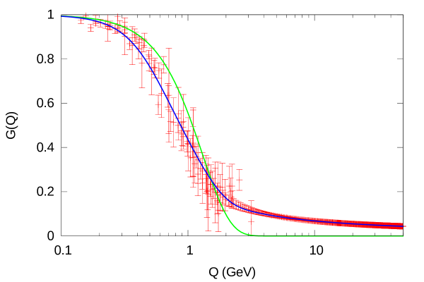
Figure 1: The function $G(Q)$ introduced in Eqs. (1) and (2). The points with error bars, in red, represent the experimentally extracted $g1$ data; the blue continous line represents $G_{g1}(Q)$, that is the fit of Eq. (14) to these data. The green continous line represents $G_{pr}(Q)$ of our previous calculations, given by Eq. (8).

The coordinate space potentials are obtained by means of Eq. (4). In particular, for the experimentally extracted data, we use the parametrization of $G_{g1}(Q)$ given in Eq. (14) with the functions $A(Q)$ and $B(Q)$ defined in Eqs. (16) and (17), respectively. The calculation is performed analytically for $A(Q)$ and numerically for $B(Q)$.

In order to display graphically the coordinate space potentials, we divide the potentials by $\alpha(0)$, introducing the following coordinate space function

$$U^{V}(r)={\frac{V^{V}(r)}{\alpha(0)}}~{}.$$ (19)

This function is plotted in Fig. 2. In more detail, in this figure, we display:

• $U_{g1}^{V}(r)$, obtained from the fit of the experimentally extracted data;

• $U_{pr}^{V}(r)$ given by Eq. (9);

• $U_{Coul}^{V}(r)$ that is given by the pure Coulombic potential of Eq. (5).

We note that, as $r\rightarrow\infty$, the three functions have the same Coulombic behavior. As $r\rightarrow 0$, $U_{pr}^{V}(r)$ takes the finite value determined by Eq. (10); numerically, this value is $U_{pr}^{V}(0)=-0.9824~{}GeV$. This regularization of the potential is given by the fastly decreasing function $G_{pr}(Q)$. On the other hand, $U_{g1}^{V}(r)$ diverges as $r\rightarrow 0$, with a slower rate than $U_{Coul}^{V}(r)$. In this respect, we observe that the function $B(Q)$ of $G_{g1}(Q)$ does not decrease sufficiently fast, as $Q\rightarrow\infty$, to regularize the corresponding coordinate space potential when $r\rightarrow 0$.

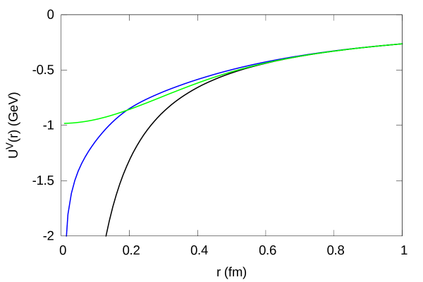
Figure 2: The coordinate space function $U^{V}(r)$ of Eq. (19). The blue line, $U_{g1}^{V}(r)$, is obtained from the fit of the experimental data; the green line, $U_{pr}^{V}(r)$ is given by the potential of the previous model; the black line, $U_{Coul}^{V}(r)$ represents the pure Coulombic case.

5 The charmonium spectrum

We can now try to reproduce the charmonium spectrum with the vector potential given by $U_{g1}^{V}(r)$.

The technique for solving the RDLE and the fit procedure are exactly the same as in Refs. [2, 5]. For the charmonium spectrum we use here the experimental data [13]. For the quality of the fit, as in [5], we define

$$\Theta=\sqrt{{\frac{\sum_{k}(E_{k}^{th}-M_{k}^{exp})^{2}}{N_{d}}}}~{},$$ (20)

where $E_{k}^{th}$ and $M_{k}^{exp}$ respectively represent the result of the theoretical calculation and the experimental value of the mass, for the $k$-th resonance and $N_{d}=16$ is the number of the fitted resonances.

We point out that the model, to reproduce accurately the spectrum, necessarily includes also a scalar $(S)$ [1, 2], or mass $(M)$ [5], interaction.

We have started the analysis trying to fix the vector interaction strength at the value $\alpha_{g1}(0)=\pi$, as given in Refs. [6, 7, 8]. But this choice did not allow to reproduce accurately the charmonium spectrum. In this respect, many trials have been performed modifying the form of the scalar or mass potentials. We have also tried to modify the form of $G(Q)$ but, in any case, the fit of the charmonium spectrum refused the value $\alpha_{g1}(0)=\pi$ of the vector interaction strength.

Subsequently, this quantity, that we denote from now on as $\alpha_{V}(0)$, has been left as a free parameter of the fit. This choice has allowed an acceptable reproduction of the charmonium spectrum, as shown in Table 1, where the theoretical and the experimental values of the resonance masses are displayed. The values of the parameters used for the interaction are given in Table 2.

In particular, for the mass of the quark we have taken the same value of the previous works [2],[5], that is $m_{q}=1.27~{}GeV$. This value represents the “running” charm quark mass in the $\overline{MS}$ scheme [13].

As discussed before, $\alpha_{V}(0)$ is determined by the fit to the spectrum. Comparing the results obtained for $\alpha_{V}(0)$ with $\alpha_{g1}(0)=\pi$, we have: $\alpha_{V}(0)=0.65~{}\alpha_{g1}(0)$ and $\alpha_{V}(0)=0.62~{}\alpha_{g1}(0)$, when the scalar or mass interaction are used, respectively. As discussed in the introduction, the nonunivocal definition of the effective charge, that affects particularly the low $Q$ region, can explain why the value $\alpha_{g1}(0)=\pi$ is not adequate for obtaining a suitable bound state quark interaction for our calculation.

With respect to Ref. [5], here the additional constant of the vector interaction $\bar{V}_{V}$ is considered as a completely free parameter: the vector interaction obtained from $G_{g1}(Q)$ does not allow to relate $\bar{V}_{V}$ to the quark vector self-energy.

Following the phenomenological model discussed in [5], we have fixed the constant $\bar{V}_{X}$, for both the scalar ($X=S$) and the mass ($X=M$) interaction at the value $\bar{V}_{X}=0.7350~{}GeV$. Also for the distance parameters $r_{X}$, the same values of [5] have been used, as shown in Table 2.

Analyzing in more detail the obtained results for the spectrum, we note that the quality of the fit is slightly worse here than in Ref. [5]. For the parameter $\Theta$ defined in Eq. (20), we have here $\Theta=36.0~{}MeV$ and $\Theta=38.0~{}MeV$ for the Scalar and Mass interaction, respectively. In Ref. [5], the corresponding values were $\Theta=13.4~{}MeV$ and $\Theta=12.8~{}MeV$. The quality of the fit can be improved if the parameters $V_{X}$ and $r_{X}$ are left as free parameters. We decided to fix these parameters at the same values of Ref. [5] to show that the vector potential obtained from $G_{g1}(Q)$ is compatible with the model for the scalar and mass interactions studied in Ref. [5] without changing their parameters.

For completeness, we also note that, as in [5], the model is unable to reproduce the resonance $\chi_{c0}(3915)$. The new experimental data [13] give, for this resonance, a mass of $3921.7\pm 1.8~{}MeV$. Our model, taking the quantum numbers $2^{3}P_{0}$, gives the mass values of $3857~{}MeV$ and $3846~{}MeV$, for the $S$ and the $M$ interactions, respectively. Our model and other quark models give a wrong order for the masses of this resonance and its partner $\chi_{c1}(3872)$.

We conclude this paper with the following considerations. The momentum dependence of the QCD experimentally extracted $\alpha_{g1}(Q)$ gives a vector interaction potential that is compatible with our quark model based on a RDLE. However, to fit accurately the spectrum, the constant of the vector interaction strength must be reduced with respect to $\alpha_{g1}(0)$. Moreover, the additional constant $\bar{V}_{V}$ to must be added to the vector potential. Finally, a scalar or mass interaction is also strictly necessary to reproduce in detail the charmonium spectrum. Further investigation is necessary to establish a deeper connection between the effective bound state quark interaction and the phenomenology related to the QCD analysis.

Acknowledgements

The author gratefully thanks Prof. A. Deur and the other authors of Refs. [6, 7, 8] for giving a complete numerical table of the experimentally extracted $\alpha_{g1}(Q)$. The data of this table are those shown in Fig. 1.

Table 1: Comparison between the experimental average values [13] of the charmonium spectrum (last column) and the theoretical results of the model. All the masses are in MeV. The quantum numbers $n$, $L$, $S$ and $J$, introduced in Ref. [2], respectively represent the principal quantum number, the orbital angular momentum, the spin and the total angular momentum. The results of the columns “Scalar” and “Mass” respectively refer to the scalar (S) and mass (M) interaction. A line divides the resonances below and above the open Charm threshold. At the bottom, the quantity $\Theta$, in $MeV$, defined in Eq. (20), gives an indication of the quality of the fit.

Name	$n^{2S+1}L_{J}$	Scalar	Mass	Experiment
$\eta_{c}(1S)$	$1^{1}S_{0}$	2989	2994	2983.9 $\pm$ 0.4
$J/\psi(1S)$	$1^{3}S_{1}$	3100	3114	3096.9 $\pm$ 0.006
$\chi_{c0}(1P)$	$1^{3}P_{0}$	3418	3407	3414.71 $\pm$ 0.30
$\chi_{c1}(1P)$	$1^{3}P_{1}$	3498	3494	3510.67 $\pm$ 0.05
$h_{c}(1P)$	$1^{1}P_{1}$	3511	3510	3525.38 $\pm$ 0.11
$\chi_{c2}(1P)$	$1^{3}P_{2}$	3558	3564	3556.17 $\pm$ 0.07
$\eta_{c}(2S)$	$2^{1}S_{0}$	3631	3626	3637.5 $\pm$ 1.1
$\psi(2S)$	$2^{3}S_{1}$	3675	3677	3686.10 $\pm$ 0.06
$\psi(3770)$	$1^{3}D_{1}$	3791	3784	3773.7 $\pm$ 0.4
$\psi_{2}(3823)$	$1^{3}D_{2}$	3823	3819	3823.7 $\pm$ 0.5
$\chi_{c1}(3872)$	$2^{3}P_{1}$	3898	3891	3871.65 $\pm$ 0.06
$\chi_{c2}(3930)$	$2^{3}P_{2}$	3932	3933	3922.5 $\pm$ 1.0
$\psi(4040)$	$3^{3}S_{1}$	4017	4018	4039 $\pm$ 1
$\chi{c1}(4140)$	$3^{3}P_{1}$	4153	4151	4146.5 $\pm$ 3.0
$\psi(4230)$	$4^{3}S_{1}$	4222	4227	4222.7 $\pm$ 2.6
$\chi{c1}(4274)$	$4^{3}P_{1}$	4284	4292	4286 $\pm$ 9
$\Theta$		$36.0$	$38.0$

Table 2: Numerical values of the parameters of the model; for more details see Sect. 5. The quark mass $m_{q}$ is fixed at the value of Ref. [13]. The constant $\alpha_{V}(0)$ represents the strength of the vector interaction; $\bar{V}_{V}$ is the additional constant of the vector interaction. The parameters of the scalar or mass interaction $\bar{V}_{X}$ and $r_{X}$ have the same values of Ref. [5].

			Units
$m_{q}$	$1.27$		GeV
	Scalar	Mass
$\alpha_{V}(0)$	$2.030$	$1.946$
$\bar{V}_{V}$	$1.837$	$1.843$	GeV
$\bar{V}_{X}$	$0.735$	$0.735$	GeV
$r_{X}$	$1.849$	$1.846$	fm

References

- [1] M. De Sanctis, Acta Phys. Pol. B 52, 125 (2021).
- [2] M. De Sanctis, Acta Phys. Pol. B 52, 1289 (2021).
- [3] M. De Sanctis, Acta Phys. Pol. B 53, 7A-2 (2022).
- [4] M. De Sanctis, Front. Phys. 7, 25 (2019).
- [5] M. De Sanctis, Acta Phys. Pol. B 54, 1A-2 (2023).
- [6] A. Deur, V. Burkert, J.P. Chen and W. Korsch, “Experimental determination of the effective strong coupling constant”, Phys.Lett. B 650, 244 (2007); arXiv:hep-ph/0509113v3, (2007).
- [7] A. Deur, V. Burkert, J.P. Chen and W. Korsch, “Determination of the effective strong coupling constant from CLAS spin structure function data”, Phys.Lett.B 665, 349 (2008); arXiv:hep-ph/0803.4119v2, (2008).
- [8] A. Deur, V. Burkert, J.P. Chen and W. Korsch, “Experimental determination of the QCD effective charge ”, Particles 5(2), 171 (2022); arXiv:2205.01169v2 [hep-ph] (2022).
- [9] A. Deur, S. J. Brodsky and C. D. Roberts, “QCD Running Couplings and Effective Charges” arXiv:2303:00723v1 [hep-ph] (2023), Review commissioned by Progress in Particle and Nuclear Physics.
- [10] A. Deur, S. J. Brodsky and G. F. de Téramond, “ The QCD running coupling”, Progress in Particle and Nuclear Physics, 90, 1 (2016).
- [11] J. L. Richardson, Phys. Lett. B 82, 272 (1979).
- [12] S. Godfrey and N. Isgur, Phys, Rev. D32 189 (1985).
- [13] R.L. Workman et al. (Particle Data Group), Prog. Theor. Exp. Phys. 2022, 083C01 (2022).