Pixel-Level Clustering Network for Unsupervised Image Segmentation

Abstract

While image segmentation is crucial in various computer vision applications, such as autonomous driving, grasping, and robot navigation, annotating all objects at the pixel-level for training is nearly impossible. Therefore, the study of unsupervised image segmentation methods is essential. In this paper, we present a pixel-level clustering framework for segmenting images into regions without using ground truth annotations. The proposed framework includes feature embedding modules with an attention mechanism, a feature statistics computing module, image reconstruction, and superpixel segmentation to achieve accurate unsupervised segmentation. Additionally, we propose a training strategy that utilizes intra-consistency within each superpixel, inter-similarity/dissimilarity between neighboring superpixels, and structural similarity between images. To avoid potential over-segmentation caused by superpixel-based losses, we also propose a post-processing method. Furthermore, we present an extension of the proposed method for unsupervised semantic segmentation. We conducted experiments on three publicly available datasets (Berkeley segmentation dataset, PASCAL VOC 2012 dataset, and COCO-Stuff dataset) to demonstrate the effectiveness of the proposed framework. The experimental results show that the proposed framework outperforms previous state-of-the-art methods.

[ ]organization=Department of Electronic Engineering, Seoul National University of Science and Technology, addressline=232 Gongneung-ro, Nowon-gu, city=Seoul, postcode=01811, country=South Korea

1 INTRODUCTION

Image segmentation is an essential task in various computer vision applications, where it groups the pixels of an input image into segments that contain pixels belonging to the same object, stuff, or component. This task plays a critical role in numerous fields, including robot navigation, grasping, and autonomous driving. Specifically, in robot navigation and autonomous driving, image segmentation is used to distinguish between ground, objects, and air in an image, ensuring safe navigation. In robot grasping, image segmentation helps in localizing the target object among other objects.

While supervised semantic segmentation has attracted significant attention from researchers because of its high accuracy (Shelhamer et al., 2017; Kang and Nguyen, 2019; Shojaiee and Baleghi, 2023), these methods typically require a large dataset consisting of images and their pixel-level class labels, which is expensive to obtain. Moreover, supervised semantic segmentation methods have limitations in handling unknown object classes since they are constrained to classify each pixel into one of the predefined categories. For instance, when a robot encounters an object that does not belong to any of the predefined classes, it is impossible to segment the object correctly.

To avoid costly pixel-level annotations and limitations of predefined classes, researchers have explored unsupervised image segmentation and unsupervised semantic segmentation (Ji et al., 2019a; Yadav and Saraswat, 2022). While unsupervised semantic segmentation usually requires a set of training images, unsupervised image segmentation can operate with only one image. This is because unsupervised semantic segmentation aims to group pixels of the same object or stuff type across multiple images. In this paper, we investigate an unsupervised image segmentation method that can segment any object or stuff using only one image and without the limitations of predefined classes.

Various pixel-level prediction tasks have achieved high accuracy through CNN-based methods (Kang et al., 2018; Nakajima et al., 2019). Consequently, unsupervised image segmentation methods have also incorporated CNNs (Xia and Kulis, 2017; Kanezaki, 2018). Since these methods lack access to annotations, Xia and Kulis (2017) proposed using image reconstruction to guide feature embedding for an image. Alternatively, Kanezaki (2018) proposed using superpixels to compute a loss. Since then, various approaches have been proposed to improve unsupervised image segmentation by avoiding using superpixel segmentations (Kim et al., 2020; Kim and Ye, 2020), utilizing both image reconstruction and superpixel segmentation (Lin et al., 2021), and by training an additional clustering module (Zhou and Wei, 2020). However, they often suffer from over-segmentation due to inconsistent features within an object caused by the losses using either superpixels or only neighboring pixels.

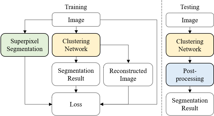
Figure 1: Illustration of the proposed framework. In training, an input image is fed into both a clustering network and a superpixel segmentation algorithm. Then, a loss is computed by using the segmentation result, superpixels, reconstructed image, and input image. In testing, superpixel segmentation and image reconstruction are not used. Hence, an input image is fed into only the clustering network to obtain an initial segmentation result. It is further processed by a post-processing method to obtain the final segmentation result.

To overcome these limitations, in this paper, we propose a novel framework that can extract more discriminative and consistent features by utilizing CNNs, image reconstruction, and superpixel segmentation, as illustrated in Figure 1. Unlike previous works, we introduce a feature embedding module (FEM) to replace typical residual blocks in CNNs. The FEM employs a channel attention mechanism and a fused activation function. Furthermore, we propose to explicitly aggregate local and global context information. Lastly, we propose a novel loss function that utilizes both superpixel segmentation and image reconstruction. The loss for image reconstruction is computed using both structural similarity (SSIM) and pixel-level similarity. The loss using superpixels considers both the internal consistency within each superpixel and the inter-similarity/dissimilarity between neighboring superpixels (see Figure 2). We evaluate the proposed framework on two public benchmark datasets (BSDS dataset (Martin et al., 2001) and PASCAL VOC 2012 dataset (Everingham et al., 2010)) for unsupervised image segmentation. The experimental results demonstrate that our proposed method outperforms the previous state-of-the-art method (Zhou and Wei, 2020).

The contributions of this paper are as follows:

• We introduce a pixel-wise clustering network that utilizes a channel-wise attention mechanism and aggregates both local and global contextual information to achieve high accuracy.

• To train the network with only a single image and without requiring any annotations, we propose a novel loss function. This function penalizes clustering pixels with similar features in neighboring superpixels into different clusters. It also penalizes classifying pixels within each superpixel into different clusters. It also uses both multi-scale structural similarity (MS-SSIM) and L2 losses.

• We propose a method for using the statistics of both deep and shallow features to measure the similarity of features between neighboring superpixels.

• We demonstrate the extended value of the proposed method by applying it to unsupervised semantic segmentation.

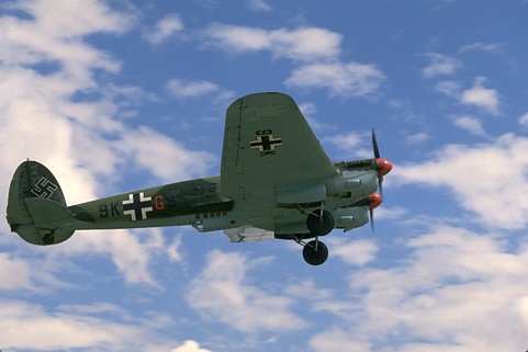
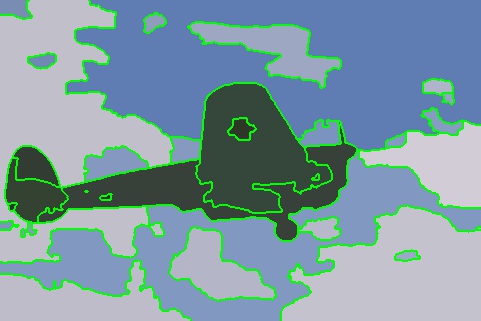
(a)

(b)

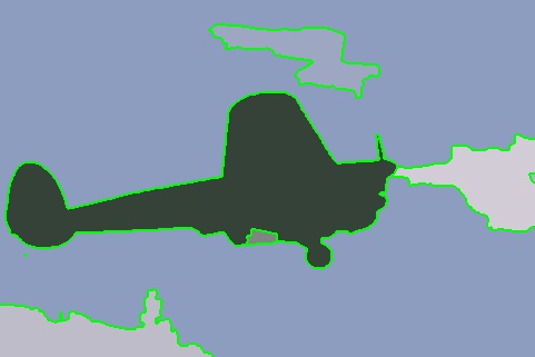
(c)

(d)

Figure 2: (a) Input image; (b) Result of the proposed network trained by using only intra-consistency $\mathcal{L}_{local}$ within each superpixel; (c) Result of the proposed network; (d) Result of the proposed framework including a graph-based post-processing method.

2 RELATED WORKS

2.1 Unsupervised Image Segmentation

As various computer vision tasks have achieved high accuracy with CNN-based methods, unsupervised image segmentation methods have also employed CNNs. One of the earliest works that utilized CNNs for unsupervised image segmentation was proposed by Xia and Kulis (2017). They introduced the W-Net, which consists of an encoder and a decoder. The network is trained by minimizing image reconstruction loss and normalized cut loss. They also employed post-processing techniques such as conditional random field (CRF) smoothing (Krähenbühl and Koltun, 2011) and hierarchical merging (Arbeláez et al., 2011) to improve the segmentation results. Another early work based on CNNs was proposed independently by Kanezaki (2018). While Xia and Kulis (2017) utilized an image reconstruction loss, Kanezaki (2018) trained the network using separately extracted superpixels. Both methods designed their networks so that each channel of the output corresponds to the probability of belonging to each cluster. Therefore, pixel-level cluster labels are obtained by finding the maximum value along the channels.

To overcome the limitations associated with losses dependent on superpixel segmentations, Kim et al. (2020) and Kim and Ye (2020) independently devised techniques that eliminate the need for superpixels. Instead of relying on a superpixel-based loss, Kim et al. (2020) employed a spatial continuity loss function that encourages neighboring pixels to be grouped together, while Kim and Ye (2020) utilized a Mumford-Shah functional-based loss function to train CNNs. Lin et al. (2021) and Zhou and Wei (2020) improved upon the previous works that relied on superpixel segmentations. Lin et al. (2021) proposed a framework that employs both an autoencoder similar to (Xia and Kulis, 2017) and superpixel segmentation like (Kanezaki, 2018). Zhou and Wei (2020) proposed a trainable clustering module that iteratively updates cluster associations and cluster centers.

In this paper, we propose a CNN-based clustering framework that utilizes both image reconstruction and superpixel segmentation to compute a loss. To extract more discriminative and consistent representations for segmentation than previous works, we replace the typical residual block with the proposed feature embedding module (FEM) and fuse local and global information using explicit multi-scaling. The FEM employs a channel-attention mechanism and a fused activation function. Unlike previous works (Xia and Kulis, 2017; Lin et al., 2021), we compute the image reconstruction loss using both patch-wise structural differences and pixel-level differences. For superpixel segmentation, unlike previous methods (Kanezaki, 2018; Zhou and Wei, 2020), we compute a loss based on both inter-similarity/dissimilarity between neighboring superpixels and intra-identity within each superpixel. Compared to the method by Lin et al. (2021), we propose additional statistics to measure inter-similarity/dissimilarity. Experimental results demonstrate that the proposed method achieves about 10% relatively higher accuracy than the previous state-of-the-art method.

2.2 Unsupervised Semantic Segmentation

Unsupervised image segmentation and unsupervised semantic segmentation serve different purposes and have different requirements. While unsupervised image segmentation clusters pixels within an image into separate regions based on instances, objects, and components, unsupervised semantic segmentation classifies pixels based on semantic classes. Accordingly, the latter usually requires a set of training images (patches) to handle semantic classes while the former can be trained using only a single image.

Despite their differences, we briefly summarize previous works on unsupervised semantic segmentation since both tasks aim to learn how to cluster pixels without ground-truth annotations. Ji et al. (2019a) introduced a technique that extracts common representations from the same objects while discarding instance-specific features by employing random transformations and spatial proximity. Cho et al. (2021b) proposed a method that uses both geometric and photometric transformations to generate multiple augmented versions of original images. Van Gansbeke et al. (2021) proposed a method that uses object mask proposals and a contrastive loss function. The method first generates object masks and then uses them to train feature embeddings. Most recently, Hamilton et al. (2022) introduced STEGO, a method that uses a pre-trained and frozen backbone to extract features, and then distills them into discrete semantic labels using contrastive learning.

Since the two tasks share some commonalities, certain approaches can be applied to both. Therefore, following the previous literature by Kim et al. (2020), we compare our proposed method to IIC (Ji et al., 2019a). Additionally, we present an extension of the proposed method for unsupervised semantic segmentation by fusing it with STEGO (Hamilton et al., 2022).

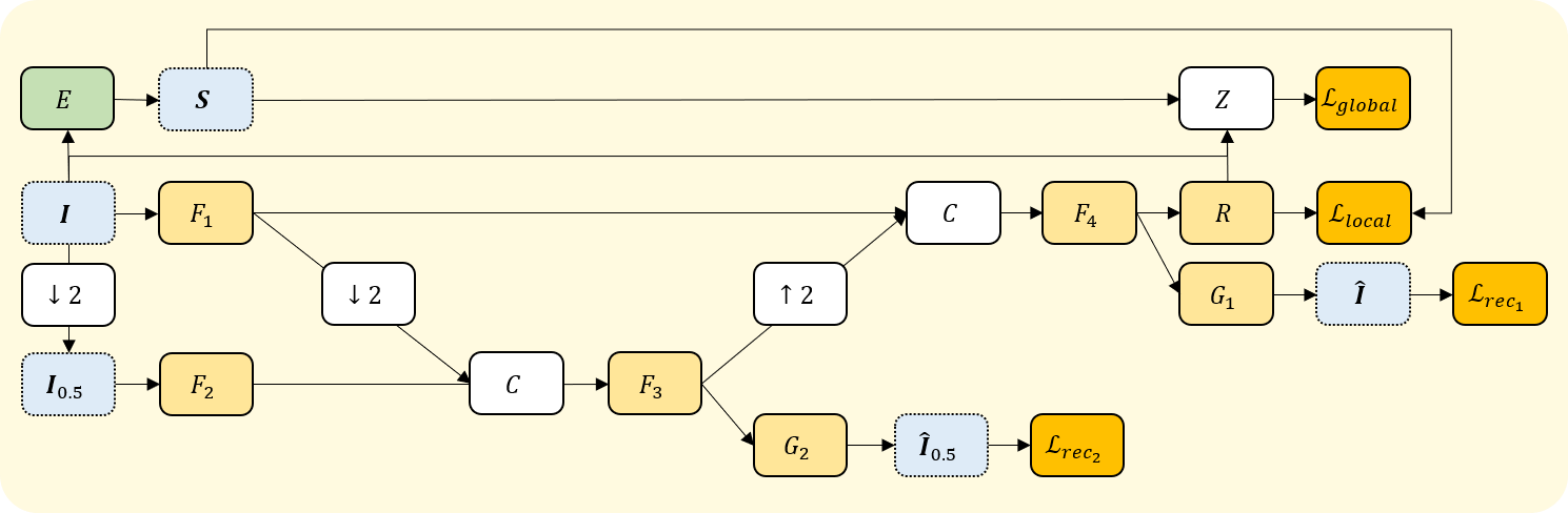
Figure 3: The proposed framework during training. $\boldsymbol{I}$, $\boldsymbol{I}_{0.5}$, and $\boldsymbol{S}$ represent an image, its downsampled image, and extracted superpixels, respectively. $E$ and ($F_{1}$, $F_{2}$, $F_{3}$, $F_{4}$) denote superpixel segmentation and four feature embedding modules, respectively. ($G_{1}$, $G_{2}$) and ($\hat{\boldsymbol{I}}$, $\hat{\boldsymbol{I}}_{0.5}$) represent two image reconstruction modules and reconstructed images, respectively. $Z$, $R$, $C$, $\downarrow 2$, and $\uparrow 2$ represent a feature statistics computing module, a cluster prediction module, concatenation, downsampling by a factor of 2, and upsampling by a factor of 2, respectively. $\mathcal{L}_{local}$ and $\mathcal{L}_{global}$ denote loss terms within a superpixel and between neighboring superpixels, respectively. $\mathcal{L}_{rec}$ denotes an image reconstruction loss.

3 PROPOSED METHOD

3.1 Pixel-level Clustering Network

The proposed framework is designed to achieve accurate unsupervised image segmentation by utilizing feature statistics, fusing local and global context features, and employing attention mechanisms, image reconstruction, explicit multi-scaling, and superpixel segmentation. An overview of the proposed framework is shown in Figure 3.

To robustly determine the merging or separating of clusters, feature statistics are computed for each superpixel using extracted features from CNNs. These statistics are then utilized to compare neighboring superpixels. The feature statistics computing module, superpixel segmentation algorithm, and extracted superpixels are denoted as $Z$, $E$, and $\boldsymbol{S}$, respectively, in Figure 3. Further details of the feature statistics computing module are described in Section 3.2.

The fusion of local and global context features is essential to achieve accurate segmentation by considering both adjacent regions and global circumstances. To accomplish this, we combine feature maps extracted at input resolution with those extracted at half of the input resolution. We perform feature extraction using four feature embedding modules ($F_{1}$, $F_{2}$, $F_{3}$, $F_{4}$ in Figure 3). Given an input image $\boldsymbol{I}$, $F_{1}$ extracts feature maps at input resolution that correspond to relatively local features. We use bicubic interpolation-based downsampling instead of a strided convolution to explicitly downsample $\boldsymbol{I}$ by 2 and extract feature maps from the downsampled image $\boldsymbol{I}_{0.5}$. The extracted maps contain relatively global features. Then, we downsample the output of $F_{1}$ by 2 using max-pooling and concatenate ($C$) it with the output of $F_{2}$. The outputs of $F_{1}$ and $F_{2}$ complement each other as the former provides more local information, and the latter contains more global representation. $F_{3}$ takes the concatenated maps and extracts representations that correspond to global context information. We concatenate the output of $F_{1}$ and the upsampled output of $F_{3}$ and process them using $F_{4}$.

The feature embedding module (FEM) combines the attention mechanism with the structure of a residual unit to achieve accurate segmentation. The attention mechanism enables the neurons to focus on significant features and suppress irrelevant representations, while the residual structure ensures stable training. Together with the explicit fusion of local and global features, these contribute to learning and extracting more robust and meaningful features for unsupervised image segmentation.

Superpixel segmentation is used to compute a loss for training the network. First, an image $\boldsymbol{I}$ is passed through a superpixel segmentation algorithm $E$ to obtain a set of superpixels $\boldsymbol{S}$. Assuming that the superpixel segmentation is accurate, a loss is then computed to ensure that the pixels within a superpixel are clustered together. As superpixels are not directly used to segment an image, minor inaccuracy in superpixel segmentation is acceptable for computing a loss to train the network. As mentioned earlier, the extracted superpixels are also used to compute feature statistics to compare neighboring superpixels.

The image reconstruction modules ($G_{1}$, $G_{2}$) guide the clustering network to encode sufficient information for robust clustering. They force the network to consider the overall content of the image at intermediate stages, rather than making clustering predictions at early layers. Each module consists of one $1\times 1$ convolution layer, which reduces the number of channels to that of color channels. We empirically demonstrate that the image reconstruction modules improve accuracy.

The followings describe more details about the training of the clustering framework. Firstly, given an image $\boldsymbol{I}$, the superpixel segmentation algorithm $E$ is applied to obtain the superpixels $\boldsymbol{S}$. Since the superpixel segmentation is not dependent on the parameters in CNNs, the superpixel extraction is performed only once per image. While any superpixel segmentation algorithm can be used, we employ Multiscale Combinatorial Grouping (MCG) (Arbeláez et al., 2014).

The clustering network is also given the image $\boldsymbol{I}$. Firstly, the image is downsampled by 2 using bicubic interpolation. Then, $F_{1}$ processes the original image, and $F_{2}$ processes the downsampled image. The output of $F_{1}$ is downsampled by 2 using max-pooling and concatenated with the output of $F_{2}$. The resulting concatenated feature maps are then processed by $F_{3}$ and upsampled by a factor of 2 using transposed convolution. Finally, the output of $F_{1}$ and that of $F_{3}$ are concatenated and processed by $F_{4}$. The outputs of $F_{1}$, $F_{2}$, $F_{3}$, and $F_{4}$ have 64, 64, 128, and 128 channels, respectively.

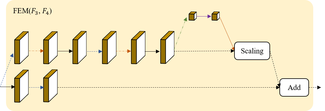
Figure 4: Architecture of feature embedding module (FEM) for $F_{3}$ and $F_{4}$. Each line and each 3D volume correspond to an operation and a feature map(vector), respectively. Black solid and dashed lines represent a convolution and an information flow, respectively. Blue dashed and orange dot-dash lines denote batch normalization and ReLU+$tanh$ activation function, respectively. Green dot-dot-dash, purple solid, and orange solid lines represent global average pooling, a 1D convolution layer, and a sigmoid function, respectively.

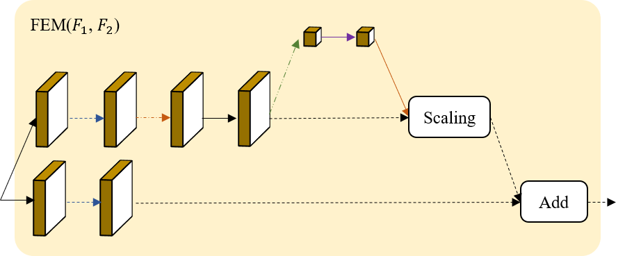
Figure 5: Architecture of feature embedding module (FEM) for $F_{1}$ and $F_{2}$. Notations are the same as Figure 4.

The FEM has a structure similar to that of a residual block (He et al., 2016c, a). In Figure 4, the bottom connection corresponds to a shortcut connection, consisting of a $3\times 3$ convolution layer and batch normalization (Ioffe and Szegedy, 2015). The middle connection is a typical stacked convolution module that contains two stacked blocks, each with batch normalization, an activation function, and a $3\times 3$ convolution layer. We use a weighted summation of ReLU and $tanh$ activation functions (Li et al., 2020) for the activation function. After the two stacked blocks, we apply an attention mechanism similar to the Efficient Channel Attention (ECA) block (Wang et al., 2020). The attention mechanism scales the output of the stacked block by a predicted significance for each channel, which is predicted by the layers presented at the top in Figure 4. These layers consist of global average pooling, a 1D convolution layer, and a sigmoid activation function. Finally, the output of the FEM is obtained by adding the output of the shortcut connection and the significance-scaled output of the stacked convolution module. Figures 4 and 5 show the structures of ($F_{3}$, $F_{4}$) and ($F_{1}$, $F_{2}$), respectively. The main differences are the absence of batch normalization and an activation function at the front of the middle connection in $F_{1}$ and $F_{2}$. Since $F_{1}$ and $F_{2}$ process images instead of feature maps, these modules do not apply them at the front.

The output of $F_{4}$ is used by $R$ to predict the probability of each pixel belonging to each cluster. To achieve this, a $1\times 1$ convolution layer and batch normalization are employed. The cluster label for each pixel is then determined by selecting the cluster with the highest probability.

3.2 Loss Function

As pixels that are close in distance and have similar features are likely to belong to the same cluster, we use the features extracted using CNNs and the spatial distance to calculate a loss. Additionally, because superpixel segmentation algorithms have been extensively studied (Achanta et al., 2012; Arbeláez et al., 2014), we use one of them as a guide to compute a loss.

The proposed loss function consists of three terms. The first term aims to ensure that pixels within each superpixel belong to the same cluster. The second term encourages neighboring superpixels to belong to the same cluster if their corresponding features are similar. The third term encodes image information in the clustering network.

To train the clustering network, we first extract superpixels from the input image $\boldsymbol{I}$. Specifically, we use Multiscale Combinatorial Grouping (MCG) (Arbeláez et al., 2014) to extract $K$ superpixels $\{S_{k}\}_{k=1}^{K}$. Then, we use the extracted superpixels to compute the loss. At each iteration, the proposed model clusters the pixels in $\boldsymbol{I}$ into multiple segments (clusters). Assuming that superpixel segmentation provides reliable results, the pixels within each superpixel should belong to the same cluster. Therefore, we find the most frequent cluster label for each superpixel and consider it as the pseudo ground-truth. We then compute the pixel-wise cross-entropy loss by comparing the output of the proposed model with the pseudo ground-truth.

In more detail, given the result of superpixel segmentation and that of the proposed model, for each superpixel $S_{k}$, the most frequent cluster $c^{m}_{k}$ is found as follows:

$$c^{m}_{k}=c^{j}\text{ where }j=\mathop{\underset{i}{\mbox{argmax}}}{|c^{i}_{k}|}$$ (1)

where $|c^{i}_{k}|$ denotes the number of pixels that belong to the cluster $c^{i}$ and are in the superpixel $S_{k}$. By utilizing the superpixel-wise most frequent cluster label $c^{m}_{k}$ found by Eq. (1), we can construct $\boldsymbol{C}^{m}_{n,q}$ that contains the pseudo ground-truth for each pixel. Then, the cross-entropy loss is computed as follows:

$$\mathcal{L}_{local}=-\sum_{n=1}^{N}\sum_{q=1}^{Q}\mathbbm{1}(\boldsymbol{C}^{m}_{n,q},q)\ln{\boldsymbol{P}_{n,q}}$$ (2)

where $Q$ denotes the number of channels of output, which corresponds to the maximum number of clusters. $\boldsymbol{P}_{n,q}$ represents the output of the model at $(n,q)$. $\mathbbm{1}(\boldsymbol{C}^{m}_{n,q},q)$ denotes an indicator function that returns one if $\boldsymbol{C}^{m}_{n,q}$ and $q$ are the same and zero otherwise. $N$ and $n$ represent the total number of pixels in $\boldsymbol{I}$ and the index for each pixel, respectively.

As $\mathcal{L}_{local}$ considers pixels in each superpixel separately, we also compute another loss term $\mathcal{L}_{global}$ to ensure that pixels are clustered together if they belong to neighboring superpixels and have similar features. The loss is computed by utilizing the feature statistics computing module.

The extracted superpixels are first used to construct a graph in which each superpixel corresponds to a node. The features ($\boldsymbol{v}_{k}$, $\boldsymbol{e}_{k}$) of each node are then calculated using the output $\boldsymbol{P}$ of the clustering network and the input image $\boldsymbol{I}$, respectively. Specifically, the deep feature $\boldsymbol{v}_{k}\in\mathbb{R}^{Q}$ is computed by summing the mean and standard deviation of the features $\boldsymbol{P}$ of the pixels that belong to the corresponding superpixel. The mean and standard deviation of the features are calculated to consider their distribution.

$$\begin{split}\boldsymbol{\mu}_{k}&=\frac{1}{|S_{k}|}\sum_{i\in S_{k}}\boldsymbol{P}_{i},\\ \boldsymbol{\sigma}_{k}&=\sqrt{\frac{1}{|S_{k}|}\sum_{i\in S_{k}}(\boldsymbol{P}_{i}-\boldsymbol{\mu}_{k})^{2}},\\ \boldsymbol{v}_{k}&=\boldsymbol{\mu}_{k}+\boldsymbol{\sigma}_{k}\end{split}$$ (3)

where $|S_{k}|$ denotes the number of pixels in the superpixel $S_{k}$. The shallow feature $\boldsymbol{e}_{k}\in\mathbb{R}^{3}$ is computed using the same method as $\boldsymbol{v}_{k}$, with $\boldsymbol{P}$ in the above equation is replaced by $\boldsymbol{I}$.

Given the nodes corresponding to superpixels, the loss is computed by taking into account the connectivity between nodes and the similarity between their features. For connectivity, nodes are connected by an edge if the corresponding superpixels are neighboring. Specifically, if any two different superpixels share a common border, the corresponding nodes are connected by an edge. For similarity, an affinity matrix $\boldsymbol{A}\in\mathbb{R}^{K\times K}$ is computed as follows:

$$\boldsymbol{A}_{i,j}=\left\{\begin{array}[]{l l}\text{exp}\Big{(}-\frac{\lVert\boldsymbol{v}_{i}-\boldsymbol{v}_{j}\rVert^{2}_{2}}{\alpha_{1}}-\frac{\lVert\boldsymbol{e}_{i}-\boldsymbol{e}_{j}\rVert^{2}_{2}}{\alpha_{2}}\Big{)},\;\text{ if }\boldsymbol{B}_{i,j}=1\\ 0,\;\text{ otherwise }\\ \end{array}\right.$$ (4)

where $\boldsymbol{B}_{i,j}$ is one if $S_{i}$ and $S_{j}$ are different and neighboring superpixels, and is zero otherwise. $\alpha_{1}$ and $\alpha_{2}$ are hyperparameters.

Then, $\mathcal{L}_{global}$ is computed as follows:

$$\mathcal{L}_{global}=\frac{1}{|\boldsymbol{A}|}tr(\boldsymbol{H}^{\text{T}}\boldsymbol{A}(\textbf{1}-\boldsymbol{H}))$$ (5)

where $|\boldsymbol{A}|$ denotes the summation of all elements in $\boldsymbol{A}$ computed by Eq. (4). $tr(\cdot)$ represents a trace operation. $\boldsymbol{H}\in\mathbb{R}^{K\times Q}$ contains the probability of the superpixel at each row belonging to the cluster at each column. Given $\boldsymbol{P}$ from the proposed model, a softmax function is firstly applied for normalization. Then, for each superpixel, the outputs of the softmax function are averaged to obtain each row of $\boldsymbol{H}$.

Image reconstruction loss $\mathcal{L}_{rec}$ consists of two MS-SSIM+$\ell_{2}$ losses introduced by Zhao et al. (2017) as follows:

$$\mathcal{L}_{rec}=\mathcal{L}_{ms\text{-}ssim+\ell_{2}}(\boldsymbol{I},\hat{\boldsymbol{I}})+\mathcal{L}_{ms\text{-}ssim+\ell_{2}}(\boldsymbol{I}_{0.5},\hat{\boldsymbol{I}}_{0.5})$$ (6)

where $\hat{\boldsymbol{I}}$ and $\hat{\boldsymbol{I}}_{0.5}$ denote the reconstructed images at the original resolution and the half resolution, respectively. The two terms on the right side are denoted by $\mathcal{L}_{rec_{1}}$ and $\mathcal{L}_{rec_{2}}$, respectively, in Figure 3. $\mathcal{L}_{ms\text{-}ssim+\ell_{2}}(\cdot,\cdot)$ is described in Eq. (7).

MS-SSIM+$\ell_{2}$ loss is a weighted summation of a MS-SSIM loss and a L2 loss. $\mathcal{L}_{ms\text{-}ssim+\ell_{2}}(\boldsymbol{I},\hat{\boldsymbol{I}})$ is computed as follows:

$$\begin{split}&\mathcal{L}_{ms\text{-}ssim+\ell_{2}}(\boldsymbol{I},\hat{\boldsymbol{I}})\\ &=\eta\mathcal{L}_{ms\text{-}ssim}(\boldsymbol{I},\hat{\boldsymbol{I}})+(1-\eta)G_{\sigma^{M}_{G}}*\mathcal{L}_{\ell_{2}}(\boldsymbol{I},\hat{\boldsymbol{I}})\end{split}$$ (7)

where $\eta$ is a weighting coefficient to balance between the MS-SSIM loss and the L2 loss. $G_{\sigma^{M}_{G}}$ represents Gaussian filters with the standard deviations of $\sigma^{M}_{G}$ for varying scales $M$. $\sigma^{1}_{G}$, $\sigma^{2}_{G}$, $\sigma^{3}_{G}$, $\sigma^{4}_{G}$, and $\sigma^{5}_{G}$ are $0.5$, $1$, $2$, $4$, and $8$, respectively. $*$ denotes a convolution operation. $\mathcal{L}_{ms\text{-}ssim}(\boldsymbol{I},\hat{\boldsymbol{I}})$ is computed as follows:

$$\mathcal{L}_{ms\text{-}ssim}(\boldsymbol{I},\hat{\boldsymbol{I}})=1-\text{MS-SSIM}(\boldsymbol{I},\hat{\boldsymbol{I}})$$ (8)

where MS-SSIM is computed by the method in (Wang et al., 2003, 2004). We refer readers to (Zhao et al., 2017) for more details.

Finally, the total loss $\mathcal{L}$ is computed by a weighted sum of $\mathcal{L}_{local}$, $\mathcal{L}_{global}$, and $\mathcal{L}_{rec}$ as follows:

$$\mathcal{L}=\mathcal{L}_{local}+\gamma_{1}\mathcal{L}_{global}+\gamma_{2}\mathcal{L}_{rec}$$ (9)

where $\gamma_{1}$ and $\gamma_{2}$ are weighting coefficients to balance three loss terms. $\mathcal{L}_{local}$, $\mathcal{L}_{global}$, and $\mathcal{L}_{rec}$ are computed by Eqs. (2), (5), and (6), respectively.

Algorithm 1 Algorithm for training process

1:Input: Input image $\boldsymbol{I}\in\mathbb{R}^{H\times W\times 3}$

2:Output: Cluster label map $\boldsymbol{I}^{*}\in\mathbb{Z}^{H\times W}$

3:Initialize the hyperparameters $\alpha_{1},\alpha_{2},\gamma_{1},\gamma_{2},K$

4:Initialize the network parameters $W$

5:Extract superpixels $\{S_{k}\}^{K}_{k=1}$

6:for $t=1$ to $T$ do

7:     Extract $\boldsymbol{P}$ from $\boldsymbol{I}$ using current $W$ in the network.

8:     Obtain $\boldsymbol{I}^{*}$ by applying argmax to $\boldsymbol{P}$.

9:     Compute loss $\mathcal{L}$ using $\boldsymbol{P}$, $\boldsymbol{I}^{*}$, $\boldsymbol{I}$, $\hat{\boldsymbol{I}}$, and $S_{k}$ by Eq. (9).

10:     Update $W$ by minimizing $L$.

11:end for

3.3 Training Process

The training process is outlined in Algorithm 1. Given an input image $\boldsymbol{I}$, we begin by extracting superpixels $S_{k}$. At each iteration $t$, we forward-propagate $\boldsymbol{I}$ through the clustering network with the current parameters $\boldsymbol{W}$. The pixel-wise clustering result $\boldsymbol{I}^{*}$ is then obtained by finding the arguments of the maxima. The loss $\mathcal{L}$ in Eq. (9) is computed by utilizing the clustering result $\boldsymbol{I}^{*}$, the network’s output $\boldsymbol{P}$, reconstructed images ($\hat{\boldsymbol{I}}$, $\hat{\boldsymbol{I}}_{0.5}$), and superpixels $S_{k}$ to update the parameters in the network through back-propagation. The optimization method used is stochastic gradient descent with momentum. The iteration is repeated for a predetermined number of iterations.

Table 1: Quantitative results on the BSDS300 dataset (Martin et al., 2001).

Methods	PRI	VoI	GCE	BDE
FH (Felzenszwalb and Huttenlocher, 2004)	0.714	3.395	0.175	16.67
NCuts (Shi and Malik, 2000)	0.724	2.906	0.223	17.15
NTP (Wang et al., 2008)	0.752	2.495	0.237	16.30
MNCut (Cour et al., 2005)	0.756	2.44	0.193	15.10
KM (Salah et al., 2011)	0.765	2.41	-	-
JSEG (Deng and Manjunath, 2001)	0.776	1.822	0.199	14.40
SDTV (Donoser et al., 2009)	0.776	1.817	0.177	16.24
Mean-Shift (Comaniciu and Meer, 2002)	0.796	1.973	0.189	14.41
TBES (Mobahi et al., 2011)	0.80	1.76	-	-
CCP (Fu et al., 2015)	0.801	2.472	0.127	11.29
MLSS (Kim et al., 2013)	0.815	1.855	0.181	12.21
gPb-owt-ucm (Arbelaez et al., 2009)	0.81	1.68	-	-
W-Net (Xia and Kulis, 2017)	0.81	1.71	-	-
SAS (Li et al., 2012)	0.832	1.685	0.178	11.29
DIC (Zhou and Wei, 2020)	0.841	1.749	0.139	10.18
Proposed	0.867	1.399	0.163	8.832

3.4 Post-processing

As the proposed clustering network is trained using superpixels along with others, the network performs well in segmenting relatively small regions. However, the network may struggle with accurately segmenting large regions, such as the background. To address this issue, a post-processing method is proposed, which involves constructing an undirected graph and using graph cuts to obtain the final segmentation result. Each cluster is represented as a node in the undirected graph, and edge weights are computed using image gradients. Finally, the edges are cut based on their weights to obtain the final segmentation.

Given the pixel-wise clustering result $\boldsymbol{I}^{*}$, an undirected graph is constructed by considering each segment $\hat{S}$ in $\boldsymbol{I}^{*}$ as a vertex. To compute edge weights, the input image $\boldsymbol{I}$ is first converted to the image $\tilde{\boldsymbol{I}}$ in the CIELAB color space. Gradients ($\boldsymbol{I}^{x}$, $\boldsymbol{I}^{y}$) are then computed along the x- and y-axes using $\tilde{\boldsymbol{I}}$.

$$\begin{split}\boldsymbol{I}^{x}=|\nabla_{x}\tilde{\boldsymbol{I}}|,\quad\boldsymbol{I}^{y}=|\nabla_{y}\tilde{\boldsymbol{I}}|\end{split}$$ (10)

where $\nabla_{x}$ and $\nabla_{y}$ denote a gradient operation along x- and y-axes, respectively. Then, edge weights are computed as follows:

$$\begin{split}\Delta_{i,j}=\left\{\begin{array}[]{l l}\|g^{x}_{i,j}+g^{y}_{i,j}\|_{1},\;\text{ if }\hat{\boldsymbol{B}}_{i,j}=1\\ \infty,\;\text{ otherwise }\\ \end{array}\right.\end{split}$$ (11)

where $g^{x}_{i,j}$ and $g^{y}_{i,j}$ are computed by Eq. (12). $\hat{\boldsymbol{B}}_{i,j}$ is one if $\hat{S}_{i}$ and $\hat{S}_{j}$ are different and neighboring segments, and is zero otherwise. $g^{x}_{i,j}$ and $g^{y}_{i,j}$ are the average of the absolute difference in the CIELAB color space between $\hat{S}_{i}$ and $\hat{S}_{j}$ along x- and y-axes, respectively. They are computed as follows:

$$\begin{split}g^{x}_{i,j}=\frac{1}{|\tilde{S}^{x}_{i,j}|}\sum_{(m,n)\in\tilde{S}^{x}_{i,j}}\boldsymbol{I}^{x}_{m,n}\\ g^{y}_{i,j}=\frac{1}{|\tilde{S}^{y}_{i,j}|}\sum_{(m,n)\in\tilde{S}^{y}_{i,j}}\boldsymbol{I}^{y}_{m,n}\\ \end{split}$$ (12)

where $\tilde{S}^{x}_{i,j}$ consists of the pixels at the boundaries between $\hat{S}_{i}$ and $\hat{S}_{j}$ along x-axis. Hence, $(m,n)\in\tilde{S}^{x}_{i,j}$ belongs to $\hat{S}_{i}$ and its neighboring pixel $(m,n+1)$ belong to $\hat{S}_{j}$. Similarly, $\tilde{S}^{y}_{i,j}$ consists of the pixels at the boundaries between $\hat{S}_{i}$ and $\hat{S}_{j}$ along y-axis. Accordingly, $(m,n)\in\tilde{S}^{y}_{i,j}$ belongs to $\hat{S}_{i}$ and its neighboring pixel $(m+1,n)$ belong to $\hat{S}_{j}$. $\boldsymbol{I}^{x}_{m,n}$ and $\boldsymbol{I}^{y}_{m,n}$ are calculated by Eq. (10).

The final segmentation result is obtained by using the graph to cut the edges with high weights. This graph-cut process involves comparing the edge weights to a predetermined threshold, and each connected component in the resulting graph forms a segment.

4 EXPERIMENTS AND RESULTS

4.1 Experimental Setting

We demonstrate the effectiveness of the proposed framework using the Berkeley Segmentation Data Set (BSDS300 and BSDS500) (Martin et al., 2001; Arbeláez et al., 2011) and the PASCAL VOC 2012 dataset (Everingham et al., 2010). The BSDS500 dataset contains 500 images, which are divided into 200 images for training, 100 for validation, and 200 for testing. The BSDS300 dataset includes only the training and validation splits of the BSDS500 dataset. For evaluation, multiple human annotators label each image in the BSDS dataset. As unsupervised image segmentation methods predict segmentation results using only a single image, they typically do not consider training/validation/test splits separately. Following previous works (Kanezaki, 2018; Zhou and Wei, 2020; Kim et al., 2020), we train and evaluate the proposed framework using each image in the datasets. For the PASCAL VOC dataset, object category labels are ignored following (Kim et al., 2020). Then, the mean Intersection over Union (mIoU) is computed by comparing the segments of the ground truth and those of the predicted results.

Considering hyperparameters, the loss terms were weighted using $\gamma_{1}=10^{-5}$ and $\gamma_{2}=0.1$. The affinity matrix was computed using $\alpha_{1}=200$ and $\alpha_{2}=400$. The output of the ReLU+$tanh$ activation function was obtained by the weighted summation of the ReLU function and the $tanh$ function, where the weights were 1 and 0.4, respectively. For the stochastic gradient descent optimization, the maximum iteration $T$, learning rate, and momentum were selected as 150, 0.05, and 0.9, respectively.

Following previous works (Zhou and Wei, 2020; Li et al., 2012), we utilized optimal image scale (OIS). The proposed framework was applied to each image using six different numbers of superpixels. Among the six results, the best one was used for evaluation. The number $K$ of superpixels were 50, 100, 150, 200, 250, and 300. Please note that superpixels were only employed to train the clustering network.

Table 2: Quantitative results on the BSDS500 dataset (Martin et al., 2001).

Methods	SC	PRI	VoI
Backprop (Kanezaki, 2018)	0.50	0.77	2.15
NCuts (Shi and Malik, 2000)	0.53	0.80	1.89
CAE-TVL (Wang et al., 2017)	0.56	0.82	2.02
Mean-Shift (Comaniciu and Meer, 2002)	0.58	0.81	1.64
MLSS (Kim et al., 2013)	0.60	0.84	1.59
DSC (Lin et al., 2021)	0.60	0.83	1.62
W-Net (Xia and Kulis, 2017)	0.62	0.84	1.60
SF (Dollár and Zitnick, 2013)	0.65	0.851	1.43
gPb-owt-ucm (Arbelaez et al., 2009)	0.65	0.862	1.41
DIC (Zhou and Wei, 2020)	0.66	0.864	1.63
Proposed	0.712	0.894	1.305

Table 3: Quantitative results on the PASCAL VOC 2012 dataset (Everingham et al., 2010).

Methods	mIoU
$k$-means clustering ($k=2$)	0.3166
$k$-means clustering ($k=17$)	0.2383
FH (Felzenszwalb and Huttenlocher, 2004) ($\tau=100$)	0.2682
FH (Felzenszwalb and Huttenlocher, 2004) ($\tau=500$)	0.3647
IIC (Ji et al., 2019a) ($k=2$)	0.2729
IIC (Ji et al., 2019a) ($k=20$)	0.2005
Backprop (Kanezaki, 2018)	0.3082
DFC (Kim et al., 2020) ($\mu=5$)	0.3520
Proposed	0.4103

(a)

(b)

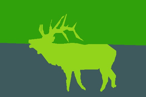
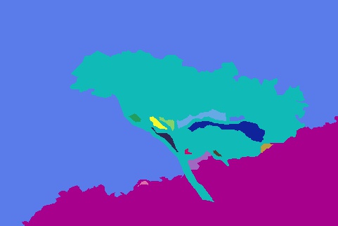
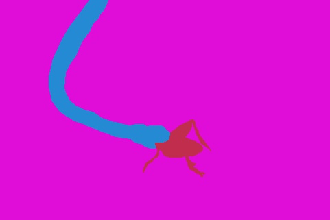
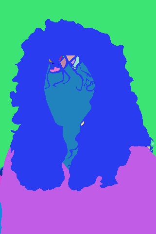
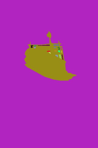
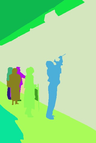
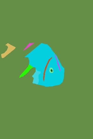
(c)

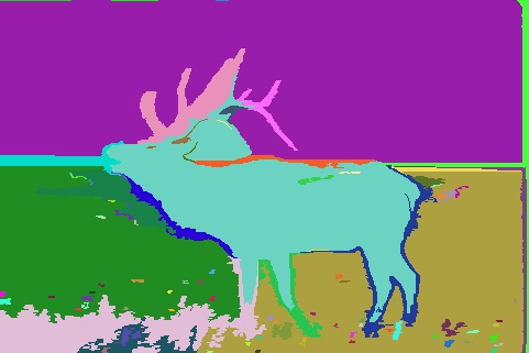
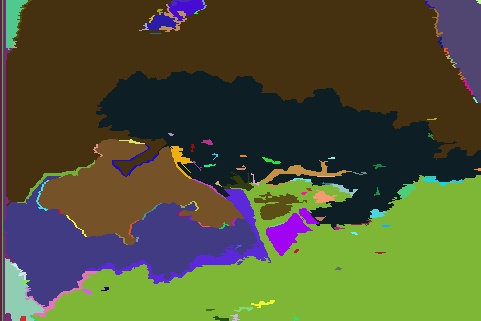
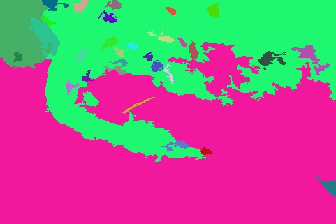
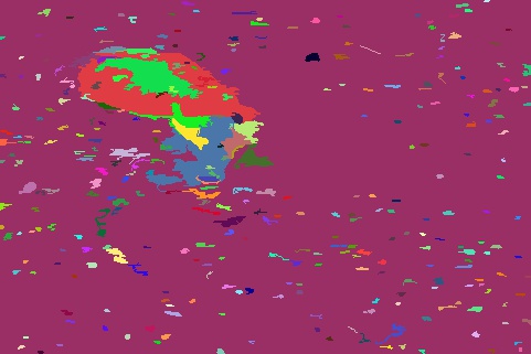
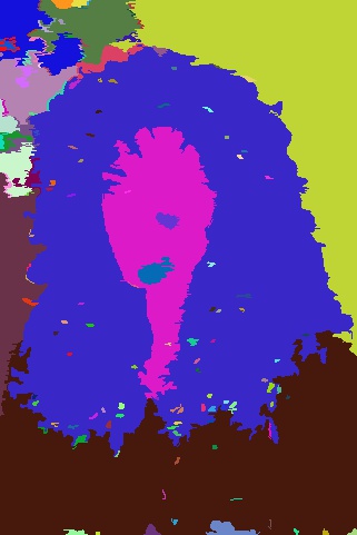
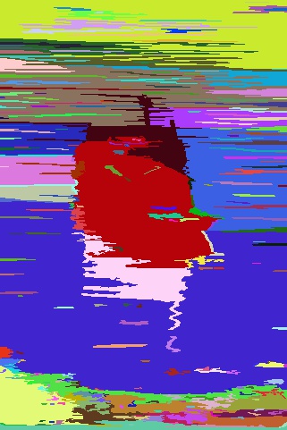
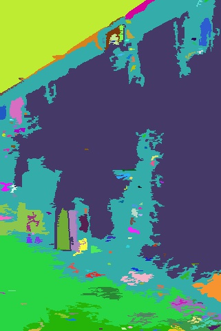
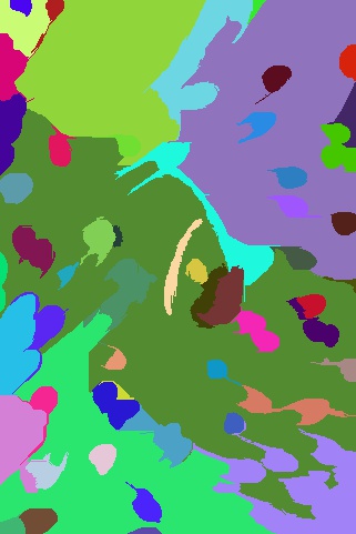
(d)

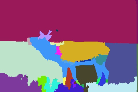
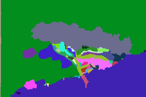
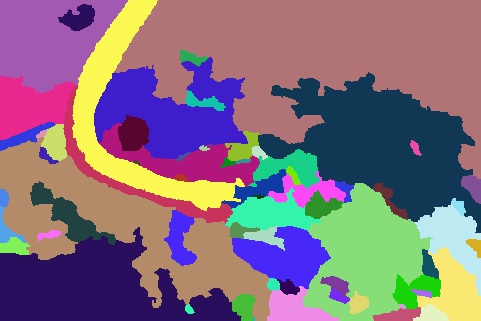
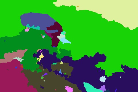
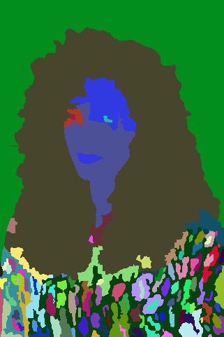
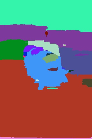
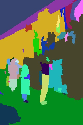
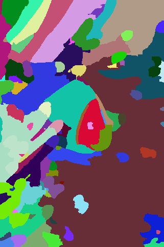
(e)

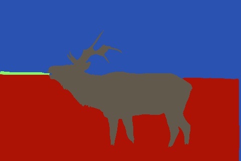
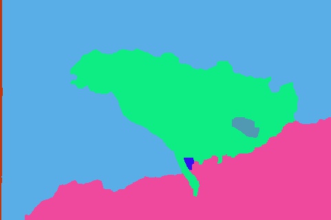
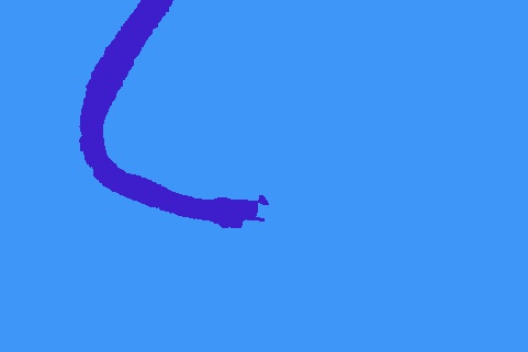
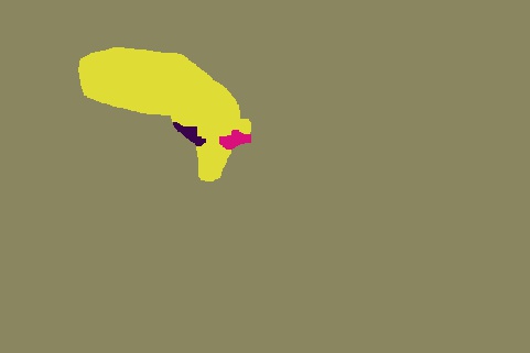
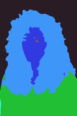
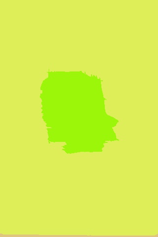
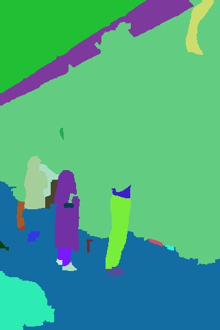
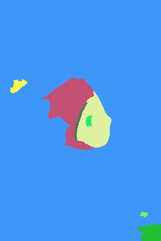
Figure 6: Qualitative results on the BSDS500 dataset (Martin et al., 2001). (a) Image; (b) Ground truth; (c) FH (Felzenszwalb and Huttenlocher, 2004); (d) DIC (Zhou and Wei, 2020); (e) Proposed method.

(a)

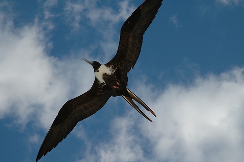
(b)

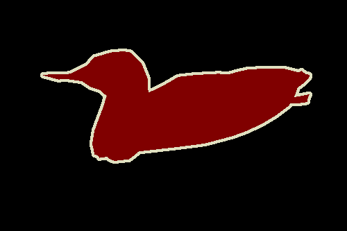
(c)

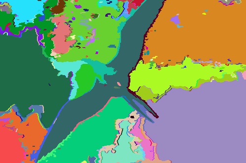
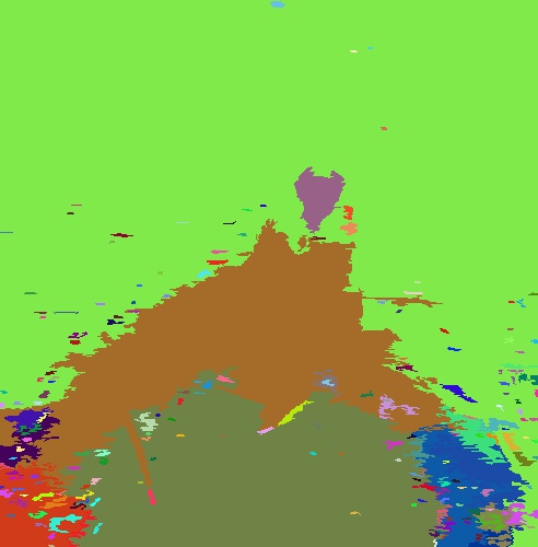
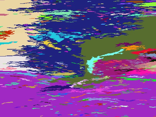
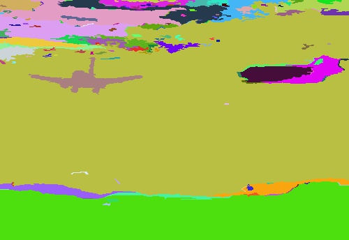
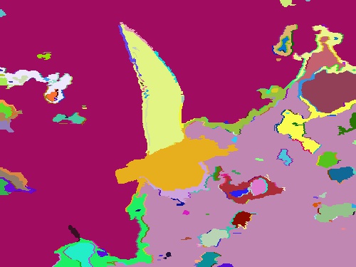
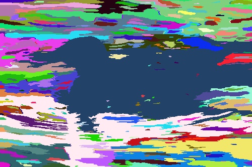
(d)

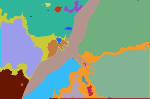
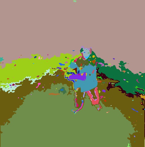
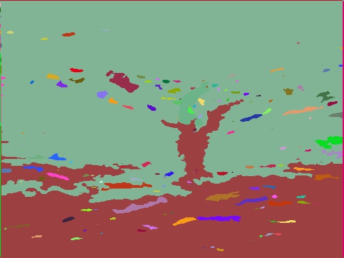
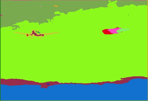
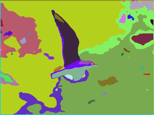
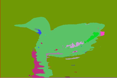
(e)

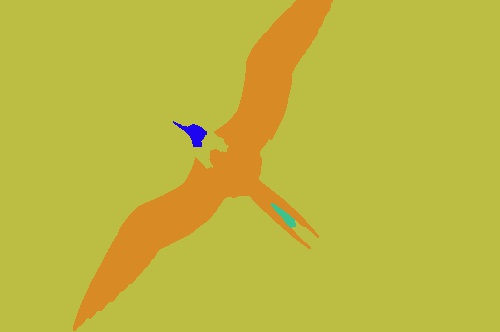
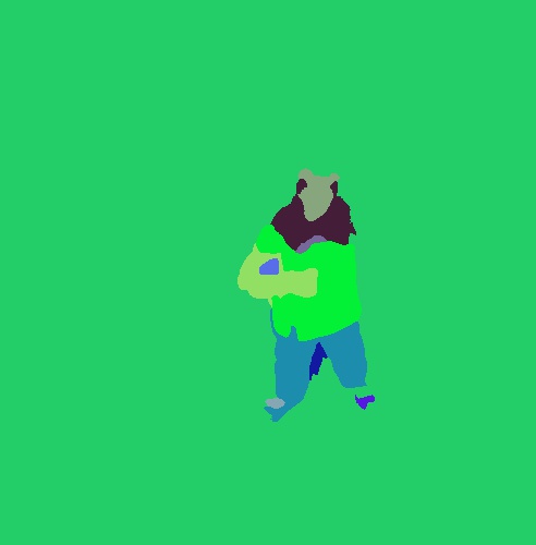
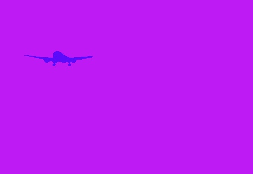
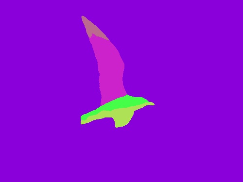
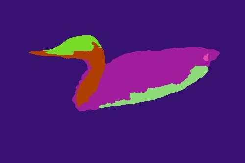
Figure 7: Qualitative results on the PASCAL VOC 2012 dataset (Everingham et al., 2010). (a) Image; (b) Ground truth; (c) FH (Felzenszwalb and Huttenlocher, 2004); (d) DFC (Kim et al., 2020); (e) Proposed method.

Table 4: Ablation study on components of the proposed framework using the BSDS300 dataset (Martin et al., 2001).

Baseline	ECA	$\mathcal{L}_{global}$	$\mathcal{L}_{rec}$	Post-processing	PRI	VoI	GCE	BDE
$\surd$					0.801	1.931	0.152	11.162
$\surd$	$\surd$				0.813	1.792	0.160	10.914
$\surd$	$\surd$	$\surd$			0.821	1.786	0.162	10.764
$\surd$	$\surd$	$\surd$	$\surd$		0.822	1.755	0.162	10.694
$\surd$	$\surd$	$\surd$	$\surd$	$\surd$	0.830	1.613	0.170	10.256

4.2 Result

For the BSDS dataset (Martin et al., 2001), we utilize five metrics that are Segmentation Covering (SC), Probabilistic Rand Index (PRI), Variation of Information (VoI), Global Consistency Error (GCE), and Boundary Displacement Error (BDE) to compare results quantitatively. Considering SC and PRI, higher scores represent better results. For VoI, GCE, and BDE, lower values denote better segmentation. Following previous works (Xia and Kulis, 2017), we use PRI, VoI, GCE, and BDE for the BSDS300 dataset and SC, PRI, and VoI for the BSDS500 dataset. As the BSDS300 dataset is a part of the BSDS500 dataset, corresponding results are quite related.

Table 1 shows quantitative results on the BSDS300 dataset (Martin et al., 2001). We compare the performance of the proposed method to those of previous methods (Kim et al., 2013; Li et al., 2012; Xia and Kulis, 2017; Fu et al., 2015; Zhou and Wei, 2020). In the table, we use boldface and underlines to denote the best and the second-best scores, respectively. The proposed method achieves the best scores in PRI, VoI, and BDE and the third-best score in GCE. The DIC method by Zhou and Wei (2020) achieves the second-best scores in PRI, GCE, and BDE. The CCP algorithm achieves the best score in GCE (Fu et al., 2015). The gPb-owt-ucm method by Arbelaez et al. (2009) achieves the second-best score in VoI.

Quantitative results on the BSDS500 dataset are shown in Table 2. The proposed method is compared to previous works (Wang et al., 2017; Kanezaki, 2018; Lin et al., 2021; Xia and Kulis, 2017; Zhou and Wei, 2020). The proposed method achieves the best scores in all metrics (SC, PRI, and VoI). The DIC method by Zhou and Wei (2020) achieves the second-best scores in SC and PRI. The gPb-owt-ucm method by Arbelaez et al. (2009) achieves the second-best score in VoI.

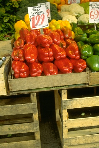
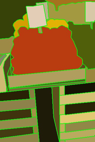
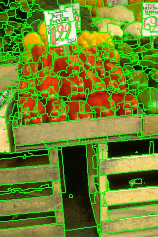
Image

Ground truth

Superpixels

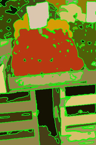
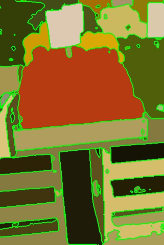
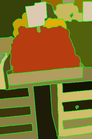
$T=50$

$T=100$

$T=150$

Figure 8: Qualitative results at the varying number of iterations.

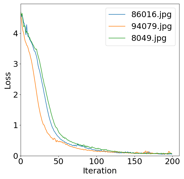
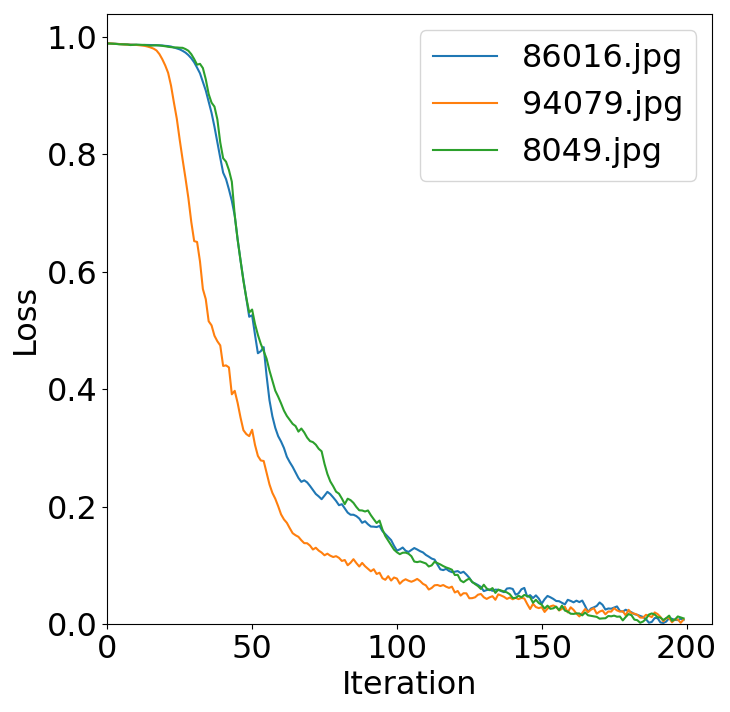
(a) $\mathcal{L}_{local}$

(b) $\mathcal{L}_{global}$

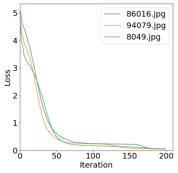
(c) $\mathcal{L}_{rec}$

Figure 9: Change of loss values during training.

We evaluated the proposed method on the PASCAL VOC 2012 dataset (Everingham et al., 2010) and computed the mean Intersection over Union (mIoU) for quantitative comparison. The results are shown in Table 3, which demonstrate that the proposed method outperforms all other methods (Felzenszwalb and Huttenlocher, 2004; Ji et al., 2019a; Kanezaki, 2018; Kim et al., 2020).

Figure 6 shows qualitative results using the BSDS500 dataset. Each row, from top to bottom, shows an input image, ground truth, and the results of FH (Felzenszwalb and Huttenlocher, 2004), DIC (Zhou and Wei, 2020), and the proposed method. Figure 7 shows qualitative results using the PASCAL VOC 2012 dataset. Each row, from top to bottom, shows an input image, ground truth, and the results of FH (Felzenszwalb and Huttenlocher, 2004), DFC (Kim et al., 2020), and the proposed method. Both qualitative results demonstrate that the proposed method achieves accurate segmentation compared to others (Felzenszwalb and Huttenlocher, 2004; Zhou and Wei, 2020; Kim et al., 2020). Moreover, the results show that the proposed method segments images into a reasonable number of clusters while other methods often produce unnecessarily over-segmented results.

Table 4 presents an ablation study on the components of the proposed framework using the BSDS300 dataset. The baseline model in Table 4 represents the framework without the attention mechanism (ECA), image reconstruction modules, and post-processing step. Also, the baseline model is trained using only $\mathcal{L}_{local}$. The first and second rows show the results of the baseline model and the model with the attention module (ECA), respectively. The third and fourth rows show the results of including $\mathcal{L}_{global}$ and $\mathcal{L}_{rec}$. The last row shows the result of the proposed framework. Please note that the scores are different from those in Table 1 because of OIS. The results in Table 1 include OIS, whereas those in Table 4 do not. In this ablation study, the number of superpixels $K$ is fixed at 100 for all the images.

To analyze the optimization process, we show the results at varying numbers of iterations in Figure 8. The figure shows the input image, ground truth, superpixel segmentation result, and results of the proposed network at 50, 100, and 150 iterations. The results in this figure do not include post-processing. We also demonstrate the convergence of loss terms by examining three different images. Figure 9 shows the change in loss values during training.

4.3 Extension to Unsupervised Semantic Segmentation

While the proposed method is designed for unsupervised image segmentation, we show the additional value of the proposed method by applying it to unsupervised semantic segmentation. Specifically, we fuse the proposed method with one of the state-of-the-art methods, STEGO (Hamilton et al., 2022), in unsupervised semantic segmentation. We then demonstrate that the fused method outperforms the previous state-of-the-art performance using the COCO-Stuff dataset (Caesar et al., 2018).

The extended method first applies the proposed method to each image to segment the image into multiple regions. Then, the image is cropped into multiple patches using the bounding boxes of segmented regions. The features of the cropped images are obtained by forward-propagating them through the pre-trained PVTv2-B5 backbone (Wang et al., 2022) and by processing mask-based pooling. The backbone is pre-trained using the self-supervised learning method by Caron et al. (2021) without any human annotations. The mask-based pooling aggregates extracted features over each segmented region. The aggregated feature is then processed by a learnable segmentation head to reduce the dimension. Finally, the centers of the $k$ clusters are determined using the outputs of the segmentation head, where $k$ is the number of semantic categories in the dataset. For clustering, the similarities are computed by the cosine distance. Unlike STEGO (Hamilton et al., 2022), conditional random field (CRF)-based refinement is not employed since the proposed method produces high-quality and detailed segmentation masks.

For evaluation and visualization, the Hungarian matching algorithm is applied to match clusters to ground-truth labels. Following STEGO (Hamilton et al., 2022), the pre-trained backbone is frozen during training while the segmentation head is trained using the contrastive loss function. Positive and negative samples are obtained by finding $k$-nearest neighbors and by random sampling, respectively. We refer readers to STEGO (Hamilton et al., 2022) for further details.

Table 5: Quantitative results on the COCO-Stuff validation dataset (Caesar et al., 2018).

Methods	Accuracy	mIoU
ResNet50 (He et al., 2016b)	24.6	8.9
MoCoV2 (Chen et al., 2020)	25.2	10.4
DINO (Caron et al., 2021)	30.5	9.6
Deep Cluster (Caron et al., 2018)	19.9	-
SIFT (Lowe, 1999)	20.2	-
AC (Ouali et al., 2020)	30.8	-
InMARS (Mirsadeghi et al., 2021)	31.0	-
IIC (Ji et al., 2019b)	21.8	6.7
MDC (Cho et al., 2021a)	32.2	9.8
PiCIE (Cho et al., 2021a)	41.1	13.8
PiCIE + H (Cho et al., 2021a)	50.0	14.4
STEGO (Hamilton et al., 2022)	56.9	28.2
Proposed	59.1	33.6

(a)

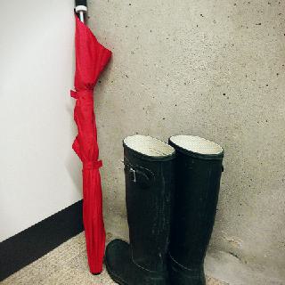
(b)

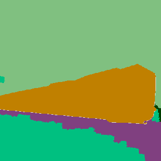
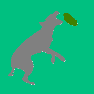
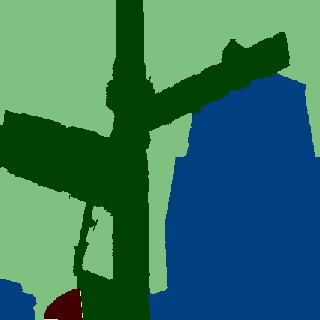
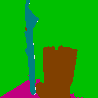
(c)

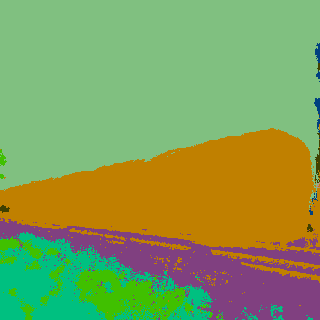
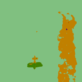
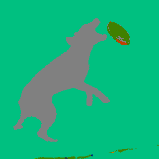
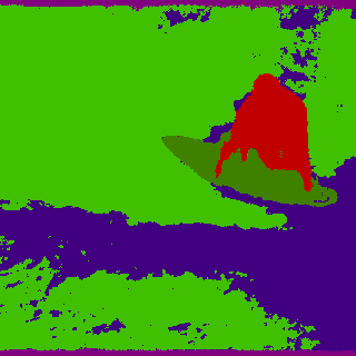
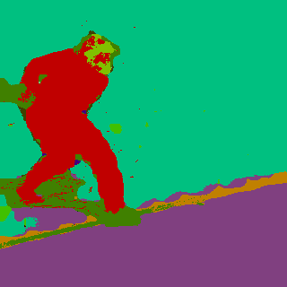
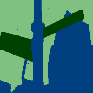
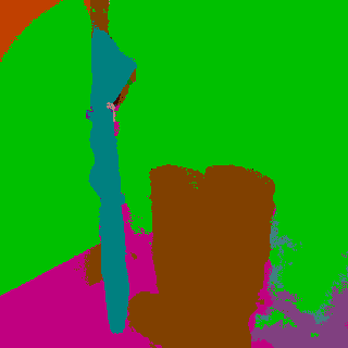
(d)

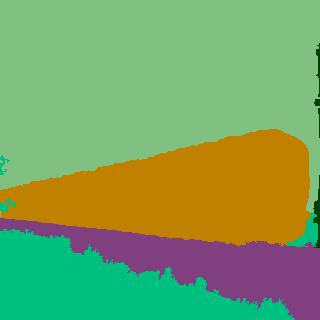
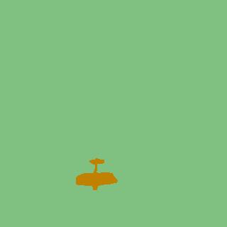
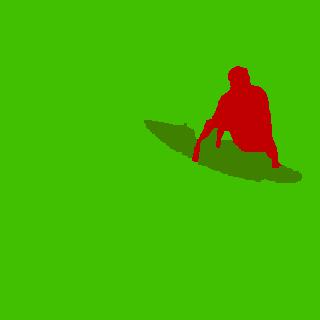
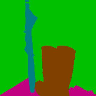
Figure 10: Qualitative results on the COCO-Stuff dataset (Caesar et al., 2018). (a) Image; (b) Ground truth; (c) STEGO (Hamilton et al., 2022); (d) Proposed method.

Following previous literature (Cho et al., 2021a), the fused method is evaluated using the 27 classes in the COCO-Stuff dataset (Caesar et al., 2018). Quantitative results demonstrate that the fused method outperforms the previous state-of-the-art method by achieving 59.1% accuracy and 33.6 mIoU, as shown in Table 5. Qualitative results are shown in Figure 10. The key difference between the fused method and STEGO (Hamilton et al., 2022) is that the fused method utilizes aggregated features over each segmented region while STEGO uses pixel-level features. We believe that given high-quality image segmentation results, the aggregated features are more consistent within each class and more discriminative between categories than pixel-level features. Moreover, since the fused method utilizes high-quality and detailed segmentation results from the proposed method, it preserves the boundaries of regions/objects better than the previous method (Hamilton et al., 2022), as shown in Figure 10.

5 CONCLUSION

We presented a novel pixel-level clustering framework for unsupervised image segmentation. The framework includes four feature embedding modules, a feature statistics computing component, two image reconstruction modules, and a superpixel segmentation algorithm. The proposed network is trained by ensuring consistency within each superpixel, utilizing feature similarity/dissimilarity between neighboring superpixels, and comparing an input image to reconstructed images from encoded features. Additionally, we included a post-processing method to overcome limitations caused by superpixels. Furthermore, we presented an extension of the proposed method for unsupervised semantic segmentation, which demonstrates the additional value of our approach. The experimental results indicate that the proposed method outperforms previous state-of-the-art methods. As the proposed framework can segment any given input image without any ground truth annotations or pre-training, it can be utilized in various real-world scenarios. For instance, it can help robots grasp unseen objects or discover new objects from a scene. Moreover, it can reduce the effort required for pixel-level annotation in supervised learning.

References

- Achanta et al. (2012) Achanta, R., Shaji, A., Smith, K., Lucchi, A., Fua, P., Süsstrunk, S., 2012. Slic superpixels compared to state-of-the-art superpixel methods. IEEE Transactions on Pattern Analysis and Machine Intelligence 34, 2274–2282. doi:10.1109/TPAMI.2012.120.
- Arbelaez et al. (2009) Arbelaez, P., Maire, M., Fowlkes, C., Malik, J., 2009. From contours to regions: An empirical evaluation, in: 2009 IEEE Conference on Computer Vision and Pattern Recognition, IEEE. pp. 2294–2301.
- Arbeláez et al. (2011) Arbeláez, P., Maire, M., Fowlkes, C., Malik, J., 2011. Contour detection and hierarchical image segmentation. IEEE Transactions on Pattern Analysis and Machine Intelligence 33, 898–916. doi:10.1109/TPAMI.2010.161.
- Arbeláez et al. (2014) Arbeláez, P., Pont-Tuset, J., Barron, J., Marques, F., Malik, J., 2014. Multiscale combinatorial grouping, in: 2014 IEEE Conference on Computer Vision and Pattern Recognition, pp. 328–335. doi:10.1109/CVPR.2014.49.
- Caesar et al. (2018) Caesar, H., Uijlings, J., Ferrari, V., 2018. Coco-stuff: Thing and stuff classes in context, in: 2018 IEEE/CVF Conference on Computer Vision and Pattern Recognition, pp. 1209–1218. doi:10.1109/CVPR.2018.00132.
- Caron et al. (2018) Caron, M., Bojanowski, P., Joulin, A., Douze, M., 2018. Deep clustering for unsupervised learning of visual features, in: Ferrari, V., Hebert, M., Sminchisescu, C., Weiss, Y. (Eds.), Computer Vision – ECCV 2018, Springer International Publishing, Cham. pp. 139–156.
- Caron et al. (2021) Caron, M., Touvron, H., Misra, I., Jegou, H., Mairal, J., Bojanowski, P., Joulin, A., 2021. Emerging properties in self-supervised vision transformers, in: 2021 IEEE/CVF International Conference on Computer Vision (ICCV), pp. 9630–9640. doi:10.1109/ICCV48922.2021.00951.
- Chen et al. (2020) Chen, X., Fan, H., Girshick, R.B., He, K., 2020. Improved baselines with momentum contrastive learning. CoRR abs/2003.04297. URL: https://arxiv.org/abs/2003.04297, arXiv:2003.04297.
- Cho et al. (2021a) Cho, J., Mall, U., Bala, K., Hariharan, B., 2021a. Picie: Unsupervised semantic segmentation using invariance and equivariance in clustering, in: 2021 IEEE/CVF Conference on Computer Vision and Pattern Recognition (CVPR), pp. 16789–16799. doi:10.1109/CVPR46437.2021.01652.
- Cho et al. (2021b) Cho, J.H., Mall, U., Bala, K., Hariharan, B., 2021b. Picie: Unsupervised semantic segmentation using invariance and equivariance in clustering, in: 2021 IEEE/CVF Conference on Computer Vision and Pattern Recognition (CVPR), pp. 16789–16799. doi:10.1109/CVPR46437.2021.01652.
- Comaniciu and Meer (2002) Comaniciu, D., Meer, P., 2002. Mean shift: a robust approach toward feature space analysis. IEEE Transactions on Pattern Analysis and Machine Intelligence 24, 603–619. doi:10.1109/34.1000236.
- Cour et al. (2005) Cour, T., Benezit, F., Shi, J., 2005. Spectral segmentation with multiscale graph decomposition, in: 2005 IEEE Computer Society Conference on Computer Vision and Pattern Recognition (CVPR’05), IEEE. pp. 1124–1131.
- Deng and Manjunath (2001) Deng, Y., Manjunath, B.S., 2001. Unsupervised segmentation of color-texture regions in images and video. IEEE transactions on pattern analysis and machine intelligence 23, 800–810.
- Dollár and Zitnick (2013) Dollár, P., Zitnick, C.L., 2013. Structured forests for fast edge detection, in: Proceedings of the IEEE international conference on computer vision, pp. 1841–1848.
- Donoser et al. (2009) Donoser, M., Urschler, M., Hirzer, M., Bischof, H., 2009. Saliency driven total variation segmentation, in: 2009 IEEE 12th International Conference on Computer Vision, pp. 817–824. doi:10.1109/ICCV.2009.5459296.
- Everingham et al. (2010) Everingham, M., Van Gool, L., Williams, C.K.I., Winn, J., Zisserman, A., 2010. The pascal visual object classes (voc) challenge. International Journal of Computer Vision 88, 303–338. URL: https://doi.org/10.1007/s11263-009-0275-4, doi:10.1007/s11263-009-0275-4.
- Felzenszwalb and Huttenlocher (2004) Felzenszwalb, P.F., Huttenlocher, D.P., 2004. Efficient graph-based image segmentation. International Journal of Computer Vision 59, 167–181. doi:10.1023/B:VISI.0000022288.19776.77.
- Fu et al. (2015) Fu, X., Wang, C.Y., Chen, C., Wang, C., Kuo, C.C.J., 2015. Robust image segmentation using contour-guided color palettes, in: Proceedings of the IEEE International Conference on Computer Vision, pp. 1618–1625.
- Hamilton et al. (2022) Hamilton, M., Zhang, Z., Hariharan, B., Snavely, N., Freeman, W.T., 2022. Unsupervised semantic segmentation by distilling feature correspondences. arXiv:2203.08414.
- He et al. (2016a) He, K., Zhang, X., Ren, S., Sun, J., 2016a. Deep residual learning for image recognition, in: 2016 IEEE Conference on Computer Vision and Pattern Recognition (CVPR), pp. 770–778. doi:10.1109/CVPR.2016.90.
- He et al. (2016b) He, K., Zhang, X., Ren, S., Sun, J., 2016b. Deep residual learning for image recognition, in: 2016 IEEE Conference on Computer Vision and Pattern Recognition (CVPR), pp. 770–778. doi:10.1109/CVPR.2016.90.
- He et al. (2016c) He, K., Zhang, X., Ren, S., Sun, J., 2016c. Identity mappings in deep residual networks, in: European conference on computer vision, Springer. pp. 630–645.
- Ioffe and Szegedy (2015) Ioffe, S., Szegedy, C., 2015. Batch normalization: Accelerating deep network training by reducing internal covariate shift, in: International conference on machine learning, PMLR. pp. 448–456.
- Ji et al. (2019a) Ji, X., Vedaldi, A., Henriques, J., 2019a. Invariant information clustering for unsupervised image classification and segmentation, in: 2019 IEEE/CVF International Conference on Computer Vision (ICCV), pp. 9864–9873. doi:10.1109/ICCV.2019.00996.
- Ji et al. (2019b) Ji, X., Vedaldi, A., Henriques, J., 2019b. Invariant information clustering for unsupervised image classification and segmentation, in: 2019 IEEE/CVF International Conference on Computer Vision (ICCV), pp. 9864–9873. doi:10.1109/ICCV.2019.00996.
- Kanezaki (2018) Kanezaki, A., 2018. Unsupervised image segmentation by backpropagation, in: 2018 IEEE International Conference on Acoustics, Speech and Signal Processing (ICASSP), pp. 1543–1547. doi:10.1109/ICASSP.2018.8462533.
- Kang et al. (2018) Kang, B., Lee, Y., Nguyen, T.Q., 2018. Depth-adaptive deep neural network for semantic segmentation. IEEE Transactions on Multimedia 20, 2478–2490. doi:10.1109/TMM.2018.2798282.
- Kang and Nguyen (2019) Kang, B., Nguyen, T.Q., 2019. Random forest with learned representations for semantic segmentation. IEEE Transactions on Image Processing 28, 3542–3555. doi:10.1109/TIP.2019.2905081.
- Kim and Ye (2020) Kim, B., Ye, J.C., 2020. Mumford–shah loss functional for image segmentation with deep learning. IEEE Transactions on Image Processing 29, 1856–1866. doi:10.1109/TIP.2019.2941265.
- Kim et al. (2013) Kim, T.H., Lee, K.M., Lee, S.U., 2013. Learning full pairwise affinities for spectral segmentation. IEEE Transactions on Pattern Analysis and Machine Intelligence 35, 1690–1703. doi:10.1109/TPAMI.2012.237.
- Kim et al. (2020) Kim, W., Kanezaki, A., Tanaka, M., 2020. Unsupervised learning of image segmentation based on differentiable feature clustering. IEEE Transactions on Image Processing 29, 8055–8068. doi:10.1109/TIP.2020.3011269.
- Krähenbühl and Koltun (2011) Krähenbühl, P., Koltun, V., 2011. Efficient inference in fully connected crfs with gaussian edge potentials, in: Shawe-Taylor, J., Zemel, R., Bartlett, P., Pereira, F., Weinberger, K.Q. (Eds.), Advances in Neural Information Processing Systems, Curran Associates, Inc.
- Li et al. (2020) Li, X., Hu, Z., Huang, X., 2020. Combine relu with tanh, in: 2020 IEEE 4th Information Technology, Networking, Electronic and Automation Control Conference (ITNEC), IEEE. pp. 51–55.
- Li et al. (2012) Li, Z., Wu, X.M., Chang, S.F., 2012. Segmentation using superpixels: A bipartite graph partitioning approach, in: 2012 IEEE conference on computer vision and pattern recognition, IEEE. pp. 789–796.
- Lin et al. (2021) Lin, Q., Zhong, W., Lu, J., 2021. Deep superpixel cut for unsupervised image segmentation, in: 2020 25th International Conference on Pattern Recognition (ICPR), pp. 8870–8876. doi:10.1109/ICPR48806.2021.9411968.
- Lowe (1999) Lowe, D., 1999. Object recognition from local scale-invariant features, in: Proceedings of the Seventh IEEE International Conference on Computer Vision, pp. 1150–1157 vol.2. doi:10.1109/ICCV.1999.790410.
- Martin et al. (2001) Martin, D., Fowlkes, C., Tal, D., Malik, J., 2001. A database of human segmented natural images and its application to evaluating segmentation algorithms and measuring ecological statistics, in: Proceedings Eighth IEEE International Conference on Computer Vision. ICCV 2001, pp. 416–423 vol.2. doi:10.1109/ICCV.2001.937655.
- Mirsadeghi et al. (2021) Mirsadeghi, S.E., Royat, A., Rezatofighi, H., 2021. Unsupervised image segmentation by mutual information maximization and adversarial regularization. IEEE Robotics and Automation Letters 6, 6931–6938. doi:10.1109/LRA.2021.3095311.
- Mobahi et al. (2011) Mobahi, H., Rao, S.R., Yang, A.Y., Sastry, S.S., Ma, Y., 2011. Segmentation of natural images by texture and boundary compression. International journal of computer vision 95, 86–98.
- Nakajima et al. (2019) Nakajima, Y., Kang, B., Saito, H., Kitani, K., 2019. Incremental class discovery for semantic segmentation with rgbd sensing, in: 2019 IEEE/CVF International Conference on Computer Vision (ICCV), pp. 972–981. doi:10.1109/ICCV.2019.00106.
- Ouali et al. (2020) Ouali, Y., Hudelot, C., Tami, M., 2020. Autoregressive unsupervised image segmentation, in: Vedaldi, A., Bischof, H., Brox, T., Frahm, J.M. (Eds.), Computer Vision – ECCV 2020, Springer International Publishing, Cham. pp. 142–158.
- Salah et al. (2011) Salah, M.B., Mitiche, A., Ayed, I.B., 2011. Multiregion image segmentation by parametric kernel graph cuts. IEEE Transactions on Image Processing 20, 545–557. doi:10.1109/TIP.2010.2066982.
- Shelhamer et al. (2017) Shelhamer, E., Long, J., Darrell, T., 2017. Fully convolutional networks for semantic segmentation. IEEE Transactions on Pattern Analysis and Machine Intelligence 39, 640–651. doi:10.1109/TPAMI.2016.2572683.
- Shi and Malik (2000) Shi, J., Malik, J., 2000. Normalized cuts and image segmentation. IEEE Transactions on Pattern Analysis and Machine Intelligence 22, 888–905. doi:10.1109/34.868688.
- Shojaiee and Baleghi (2023) Shojaiee, F., Baleghi, Y., 2023. Efaspp u-net for semantic segmentation of night traffic scenes using fusion of visible and thermal images. Engineering Applications of Artificial Intelligence 117, 105627. doi:https://doi.org/10.1016/j.engappai.2022.105627.
- Van Gansbeke et al. (2021) Van Gansbeke, W., Vandenhende, S., Georgoulis, S., Van Gool, L., 2021. Unsupervised semantic segmentation by contrasting object mask proposals, in: 2021 IEEE/CVF International Conference on Computer Vision (ICCV), pp. 10032–10042. doi:10.1109/ICCV48922.2021.00990.
- Wang et al. (2017) Wang, C., Yang, B., Liao, Y., 2017. Unsupervised image segmentation using convolutional autoencoder with total variation regularization as preprocessing, in: 2017 IEEE International Conference on Acoustics, Speech and Signal Processing (ICASSP), IEEE. pp. 1877–1881.
- Wang et al. (2008) Wang, J., Jia, Y., Hua, X.S., Zhang, C., Quan, L., 2008. Normalized tree partitioning for image segmentation, in: 2008 IEEE Conference on Computer Vision and Pattern Recognition, IEEE. pp. 1–8.
- Wang et al. (2020) Wang, Q., Wu, B., Zhu, P., Li, P., Zuo, W., Hu, Q., 2020. Eca-net: Efficient channel attention for deep convolutional neural networks, in: 2020 IEEE/CVF Conference on Computer Vision and Pattern Recognition (CVPR), pp. 11531–11539. doi:10.1109/CVPR42600.2020.01155.
- Wang et al. (2022) Wang, W., Xie, E., Li, X., Fan, D.P., Song, K., Liang, D., Lu, T., Luo, P., Shao, L., 2022. Pvt v2: Improved baselines with pyramid vision transformer. Computational Visual Media 8, 415–424. URL: https://doi.org/10.1007/s41095-022-0274-8, doi:10.1007/s41095-022-0274-8.
- Wang et al. (2004) Wang, Z., Bovik, A., Sheikh, H., Simoncelli, E., 2004. Image quality assessment: from error visibility to structural similarity. IEEE Transactions on Image Processing 13, 600–612. doi:10.1109/TIP.2003.819861.
- Wang et al. (2003) Wang, Z., Simoncelli, E., Bovik, A., 2003. Multiscale structural similarity for image quality assessment, in: The Thrity-Seventh Asilomar Conference on Signals, Systems & Computers, 2003, pp. 1398–1402. doi:10.1109/ACSSC.2003.1292216.
- Xia and Kulis (2017) Xia, X., Kulis, B., 2017. W-net: A deep model for fully unsupervised image segmentation. CoRR abs/1711.08506. URL: http://arxiv.org/abs/1711.08506, arXiv:1711.08506.
- Yadav and Saraswat (2022) Yadav, N.K., Saraswat, M., 2022. A novel fuzzy clustering based method for image segmentation in rgb-d images. Engineering Applications of Artificial Intelligence 111, 104709. doi:https://doi.org/10.1016/j.engappai.2022.104709.
- Zhao et al. (2017) Zhao, H., Gallo, O., Frosio, I., Kautz, J., 2017. Loss functions for image restoration with neural networks. IEEE Transactions on Computational Imaging 3, 47–57. doi:10.1109/TCI.2016.2644865.
- Zhou and Wei (2020) Zhou, L., Wei, W., 2020. Dic: Deep image clustering for unsupervised image segmentation. IEEE Access 8, 34481–34491. doi:10.1109/ACCESS.2020.2974496.