On the Foundations of Shortcut Learning

Abstract

Deep-learning models can extract a rich assortment of features from data. Which features a model uses depends not only on predictivity—how reliably a feature indicates train-set labels—but also on availability—how easily the feature can be extracted, or leveraged, from inputs. The literature on shortcut learning has noted examples in which models privilege one feature over another, for example texture over shape and image backgrounds over foreground objects. Here, we test hypotheses about which input properties are more available to a model, and systematically study how predictivity and availability interact to shape models’ feature use. We construct a minimal, explicit generative framework for synthesizing classification datasets with two latent features that vary in predictivity and in factors we hypothesize to relate to availability, and quantify a model’s shortcut bias—its over-reliance on the shortcut (more available, less predictive) feature at the expense of the core (less available, more predictive) feature. We find that linear models are relatively unbiased, but introducing a single hidden layer with ReLU or Tanh units yields a bias. Our empirical findings are consistent with a theoretical account based on Neural Tangent Kernels. Finally, we study how models used in practice trade off predictivity and availability in naturalistic datasets, discovering availability manipulations which increase models’ degree of shortcut bias. Taken together, these findings suggest that the propensity to learn shortcut features is a fundamental characteristic of deep nonlinear architectures warranting systematic study given its role in shaping how models solve tasks.

1 Introduction

Natural data domains provide a rich, high-dimensional input from which deep-learning models can extract a variety of candidate features. During training, models determine which features to rely on. Following training, the chosen features determine how models generalize. A challenge for machine learning arises when models come to rely on spurious or shortcut features instead of the core or defining features of a domain (Arjovsky et al., 2019; McCoy et al., 2019; Geirhos et al., 2020; Singla & Feizi, 2022). Shortcut “cheat” features, which are correlated with core “true” features in the training set, obtain good performance on the training set as well as on an iid test set, but poor generalization on out-of-distribution inputs. For instance, ImageNet-trained CNNs classify primarily according to an object’s texture (Baker et al., 2018; Geirhos et al., 2018a; Hermann et al., 2020), whereas people define and classify solid objects by shape (e.g., Landau et al., 1988). Focusing on texture leads to reliable classification on many images but might result in misclassification of, say, a hairless cat, which has wrinkly skin more like that of an elephant. The terms “spurious” and “shortcut” are largely synonymous in the literature, although the former often refers to features that arise unintentionally in a poorly constructed dataset, and the latter to features easily latched onto by a model. In addition to a preference for texture over shape, other common shortcut features include a propensity to classify based on image backgrounds rather than foreground objects (Beery et al., 2018; Sagawa et al., 2020a; Xiao et al., 2020; Moayeri et al., 2022), or based on individual diagnostic pixels rather than higher-order image content (Malhotra et al., 2020).

The literature examining feature use has often focused on predictivity—how well a feature indicates the target output. Anomalies have been identified in which networks come to rely systematically on one feature over another when the features are equally predictive, or even when the preferred feature has lower predictivity than the non-preferred feature (Beery et al., 2018; Pérez et al., 2018; Tachet et al., 2018; Arjovsky et al., 2019; McCoy et al., 2019; Hermann & Lampinen, 2020; Shah et al., 2020; Nagarajan et al., 2020; Pezeshki et al., 2021; Fel et al., 2023). Although we lack a general understanding of the cause of such preference anomalies, several specific cases have been identified. For example, features that are linearly related to classification labels are preferred by models over features that require nonlinear transforms (Hermann & Lampinen, 2020; Shah et al., 2020). Another factor leading to anomalous feature preferences is the redundancy of representation, e.g., the size of the pixel footprint in an image (Sagawa et al., 2020a; Wolff & Wolff, 2022; Tartaglini et al., 2022).

Because predictivity alone is insufficient to explain feature reliance, here we explicitly introduce the notion of availability to refer to the factors that influence the likelihood that a model will use a feature more so than a purely statistical account would predict. A more-available feature is easier for the model to extract and leverage. Past research has systemtically manipulated predictivity; in the present work, we systematically manipulate both predictivity and availability to better understand their interaction and to characterize conditions giving rise to shortcut learning. Our contributions are:

• We define quantitative measures of predictivity and availability using a generative framework that allows us to synthesize classification datasets with latent features having specified predictivity and availability. We introduce two notions of availability relating to singular values and nonlinearity of the data generating process, and quantify shortcut bias in terms of how a learned classifier deviates from an optimal classifier in its feature reliance.

• We perform parametric studies of latent-feature predictivity and availability, and examine the sensitivity of different model architectures to shortcut bias, finding that it is greater for nonlinear models than linear models, and that model depth amplifies bias.

• We present a theoretical account based on Neural Tangent Kernels (Jacot et al., 2018) which indicates that shortcut bias is an inevitable consequence of nonlinear architectures.

• We show that vision architectures used in practice can be sensitive to non-core features beyond their predictive value, and show a set of availability manipulations of naturalistic images which push around models’ feature reliance.

2 Related work

The propensity of models to learn spurious (Arjovsky et al., 2019) or shortcut (Geirhos et al., 2020) features arises in a variety of domains (Heuer et al., 2016; Gururangan et al., 2018; McCoy et al., 2019; Sagawa et al., 2020a) and is of interest from both a scientific and practical perspective. Existing work has sought to understand the extent to which this tendency derives from the statistics of the training data versus from model inductive bias (Neyshabur et al., 2014; Tachet et al., 2018; Pérez et al., 2018; Rahaman et al., 2019; Arora et al., 2019; Geirhos et al., 2020; Sagawa et al., 2020b, a; Pezeshki et al., 2021; Nagarajan et al., 2021), for example a bias to learn simple functions (Tachet et al., 2018; Pérez et al., 2018; Rahaman et al., 2019; Arora et al., 2019). Hermann & Lampinen (2020) found that models preferentially represent one of a pair of equally predictive image features, typically whichever feature had been most linearly decodable from the model at initialization. They also identified cases where models relied on a less-predictive feature that had a linear relationship to task labels over a more-predictive feature that had a nonlinear relationship to labels. Together, these findings suggest that predictivity alone is not the only factor that determines model representations and behavior. A theoretical account by Pezeshki et al. (2021) studied a situation in supervised learning in which minimizing cross-entropy loss captures only a subset of predictive features, while other relevant features go unnoticed. They introduced a formal notion of strength that determines which features are likely to dominate a solution. Their notion of strength confounds predictivity and availability, the two concepts which we aim to disengangle in the present work.

Work in the vision domain has studied which features vision models rely on when trained on natural image datasets. For example, ImageNet models prefer to classify based on texture rather than shape (Baker et al., 2018; Geirhos et al., 2018a; Hermann et al., 2020) and local rather than global image content (Baker et al., 2020; Malhotra et al., 2020), marking a difference from how people classify images (Landau et al., 1988; Baker et al., 2018). Other studies have found that image backgrounds play an outsize role in driving model predictions (Beery et al., 2018; Sagawa et al., 2020a; Xiao et al., 2020). Two studies manipulated the quantity of a feature in an image to test how this changed model behavior. Tartaglini et al. (2022) probed pretrained models with images containing a shape consistent with one class label and a texture consistent with another, where the texture was present throughout the image, including in the background. They varied the opacity of the background and found that as the the texture became less salient, models increasingly classified by shape. Wolff & Wolff (2022) found that when images had objects with opposing labels, models preferred to classify by the object with the larger pixel footprint, an idea we return to in Section 5. The development of methods for reducing bias for particular features over others is an active area (e.g. Arjovsky et al., 2019; Geirhos et al., 2018a; Hermann et al., 2020; Robinson et al., 2021; Minderer et al., 2020; Sagawa et al., 2020b; Ryali et al., 2021; Kirichenko et al., 2022; Teney et al., 2022; Tiwari & Shenoy, 2023; Ahmadian & Lindsten, 2023; Pezeshki et al., 2021; Puli et al., 2023; LaBonte et al., 2023), important for improving model generalization and addressing fairness concerns (Zhao et al., 2017; Buolamwini & Gebru, 2018).

3 Generative procedure for synthetic datasets

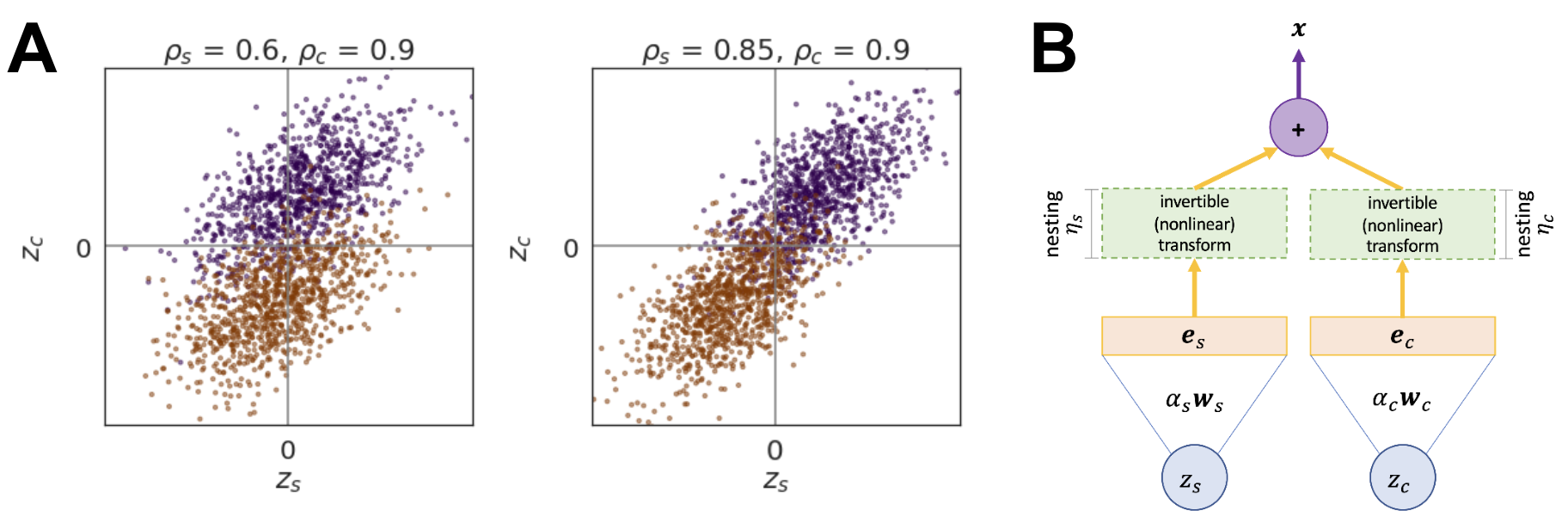
Figure 1: Synthetic data. A: Two datasets differing in the predictivity of $z_{s}$. B: Schematic of the embedding procedure manipulating availability via the mapping from $\boldsymbol{z}$ to $\boldsymbol{x}$. Dashed boxes are optional.

To systematically explore the role of predictivity and availability, we construct synthetic datasets from a generative procedure that maps a pair of latent features, $\boldsymbol{z}=(z_{s},z_{c})$, to an input vector $\boldsymbol{x}\in\mathbb{R}^{d}$ and class label $y\in\{-1,+1\}$. The subscripts $s$ and $c$ denote the latent dimensions that will be treated as the potential shortcut and core feature, respectively. The procedure draws $\boldsymbol{z}$ from a multivariate Gaussian conditioned on class,

$$\boldsymbol{z}\,|\,y\sim\mathcal{N}\left(\begin{bmatrix}y\,\mu_{s}\\ y\,\mu_{c}\end{bmatrix},\begin{bmatrix}1&\sigma_{sc}\\ \sigma_{sc}&1\end{bmatrix}\right),$$

with $|\sigma_{sc}|<1$. Through symmetry, the optimal decision boundary for latent feature $i$ is $z_{i}=0$, allowing us to define the feature predictivity $\rho_{i}\equiv\Pr(y=\textrm{sign}(z_{i}))$. For Gaussian likelihoods, this predictivity is achieved by setting $\displaystyle\mu_{i}=\sqrt{2}~{}\mathrm{erf}^{-1}\left(2\rho_{i}-1\right)$. Figure 1A shows sample latent-feature distributions for different levels of $\rho_{s}$ and $\rho_{c}$.

Availability manipulations. Given a latent vector $\boldsymbol{z}$, we manipulate the hypothesized availability (hereafter, simply availability) of each feature independently through an embedding procedure, sketched in Figure 1B, that yields an input $\boldsymbol{x}\in\mathbb{R}^{d}$. We posit two factors that influence availability of feature $i$, its amplification $\alpha_{i}$ and its nesting $\eta_{i}$. Amplification $\alpha_{i}$ is a scaling factor on an embedding, $\boldsymbol{e}_{i}=\alpha_{i}\boldsymbol{w}_{i}z_{i}$, where $\boldsymbol{w}_{i}\in\mathbb{R}^{d}$ is a feature-specific random unit vector. Amplification includes manipulations of redundancy (replicating a feature) and magnitude (increasing a feature’s dynamic range). Nesting $\eta_{i}$ is a factor that determines ease of recovery of a latent feature from an embedding. We assume a nonlinear, rank-preserving transform, $\boldsymbol{e}^{\prime}_{i}=f_{\eta_{i}}(\boldsymbol{e})$, where $f_{\eta_{i}}$ is a fully connected, random net with $\eta_{i}\in\mathbb{N}$ tanh layers in cascade. For $\eta_{i}=0$, feature $i$ remains in explicit form, $\boldsymbol{e}^{\prime}_{i}=\boldsymbol{e}_{i}$; for $\eta_{i}>0$, the feature is recoverable through an inversion of increasing complexity with $\eta_{i}$. To complete the data generative process, we combine embeddings by summation: $\boldsymbol{x}=\boldsymbol{e}^{\prime}_{s}+\boldsymbol{e}^{\prime}_{c}$.

Assessing reliance on shortcut features. Given a synthetic dataset and a model trained on this dataset, we assess the model’s reliance on the shortcut feature, i.e., the extent to which the model uses this feature as a basis for classification decisions. When $z_{c}$ and $z_{s}$ are correlated ($\sigma_{sc}>0$), some degree of reliance on the shortcut feature is Bayes optimal (see orange dashed line in Figure 6B). Consequently, we need to assess reliance relative to that of an optimal classifier. We perform this assessment in latent space, where the Bayes optimal classifier can be found by linear discriminant analysis (LDA) (see Figure 2 inset). The shortcut bias is the reliance of a model on the shortcut feature over that of the optimal, LDA:

$$\textit{bias}=\textit{reliance}_{\text{model}}-\textit{reliance}_{\text{optimal}}.$$

Appendix C.1 describes and justifies our reliance measure in detail. For a given model $\mathcal{M}$, whether trained net or LDA, we probe over the latent space and determine for each probe $\boldsymbol{z}$ the binary classification decision, $\hat{y}_{\mathcal{M}(\boldsymbol{z})}$ (see Figure 2). Shortcut reliance is the difference between the model’s alignment (covariance) with decision boundaries based only on the shortcut and core features:

$$\textit{reliance}_{\mathcal{M}}=\mathbb{E}_{\boldsymbol{z}}[\,\hat{y}_{\mathcal{M}(\boldsymbol{z})}\,(\text{sign}(z_{s})-\text{sign}(z_{c}))]$$

The reliance score is in $[-1,+1]$, though in practice (due to the construction of the datasets), it varies in $[0,1]$. And because the trained net will typically have more reliance on the shortcut feature than LDA, the shortcut bias will lie in $[0,1]$ as well.

4 Experiments manipulating feature predictivity and availability

Methodology. Using the procedure described in Section 3, we conduct controlled experiments examining how feature availability and predictivity and model architecture affect the shortcut bias. We sample class-balanced datasets with 3200 train instances, 1000 validation instances, and 900 probe (evaluation) instances that uniformly cover the $(z_{s},z_{c})$ space by taking a Cartesian product of 30 $z_{s}$ evenly spaced in $[-3\mu_{s},+3\mu_{s}]$ and 30 $z_{c}$ evenly spaced in $[-3\mu_{c},+3\mu_{c}]$. In all simulations, we set $d=100$, $\eta_{c}=\eta_{s}=0$, $\rho_{c}=0.9$, $\sigma_{sc}=0.6$. We manipulate shortcut-feature predictivity with the constraint that it is lower than core-feature predictivity but still predictive, i.e., $0.5<\rho_{s}<\rho_{c}=0.9$. Because only the relative amplification of features matters, we vary the ratio $\alpha_{s}/\alpha_{c}$, with the shortcut feature more available, i.e., $\alpha_{s}/\alpha_{c}\geq 1$. We report the means across 10 runs (Appendix C.3).

Models prefer the more available feature, even when it is less predictive. We first test whether models prefer $z_{s}$ when it is more available than $z_{c}$, including when it is less predictive, while holding model architecture fixed (see Appendix C.3). Figure 2 shows that when predictivity of the two features is matched ($\rho_{c}=\rho_{s}=0.9$), models prefer the more-available feature. And given sufficiently high availability, models can prefer the less-predictive but more-available shortcut feature to the more-predictive but less-available core feature. Availability can override predictivity.

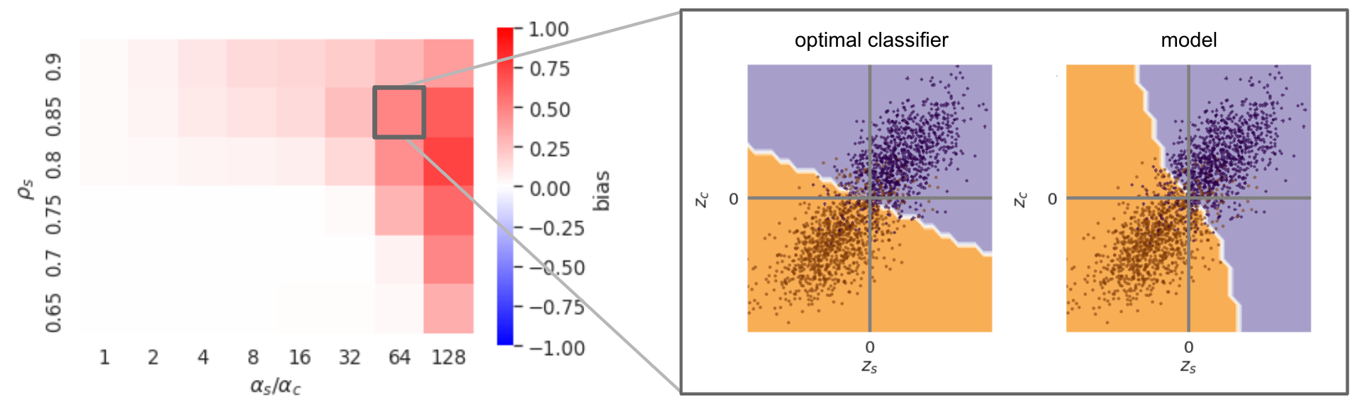
Figure 2: Deep nonlinear models can prefer a less-predictive but more-available feature to a more-predictive but less-available one. The color of each cell in the heatmap indicates the mean bias of a model as a function of the availability and predictivity of the shortcut feature, $z_{s}$. The inset shows in faint coloring the decision surface for an optimal Bayes classifier (LDA) and a trained model. Overlaid points are a subset of training instances. The model obtains a shortcut bias of $0.53$.

Model depth increases shortcut bias. In the previous experiment, we used a fixed model architecture. Here, we investigate how model depth and width influence shortcut bias when trained with $\alpha_{s}/\alpha_{c}=64$ and $\rho_{s}=0.85$, previously shown to induce a bias (see Figure 2, gray square). As shown in Figure 3A, we find that bias increases as a function of model depth when dataset is held fixed.

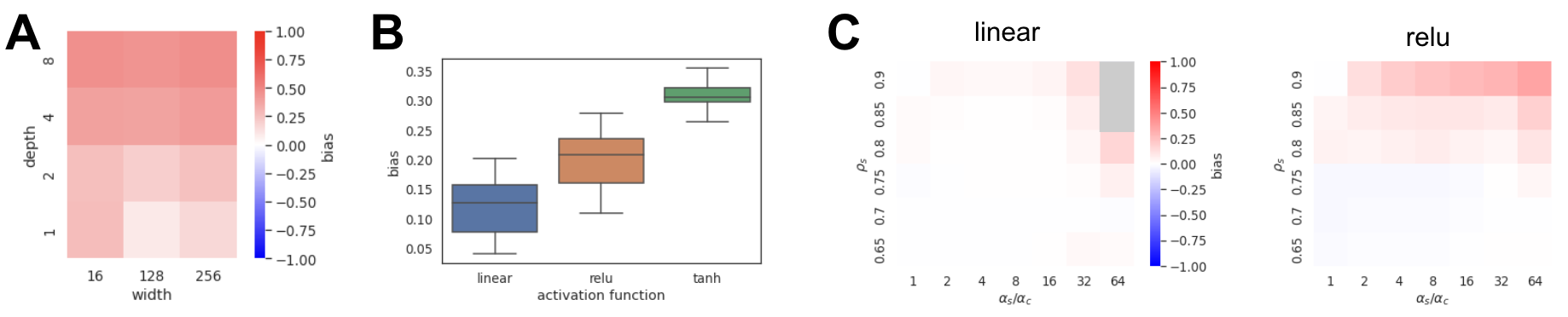
Figure 3: A: Model depth increases shortcut bias. The color of each cell indicates the mean bias of an MLP with ReLU hidden activation-functions, for various model widths and depths, trained on data with a shortcut feature that is more available ($\alpha_{s}/\alpha_{c}=64$) but less predictive ($\rho_{s}=0.85$) than the core feature. Model nonlinearity increases shortcut bias. B: Shortcut bias for three hidden activation functions for a deep MLP with width 128 and depth 2, trained on datasets where predictivity is matched ($\rho_{s}=\rho_{c}=0.9$), but shortcut availability is higher ($\alpha_{s}/\alpha_{c}=32$). A shortcut bias is more pronounced when the model contains a nonlinear activation function. C: Shortcut bias for MLPs with a single hidden layer and a hidden activation function that is either linear (left) or ReLU (right), for various shortcut feature availabilities ($\alpha_{s}/\alpha_{c}$) and predictivities ($\rho_{s}$). See B.1 for Tanh.

Model nonlinearity increases shortcut bias. To understand the role of the hidden-layer activation function, we compare models with linear, ReLU, and Tanh activations while holding weight initialization and data fixed. As indicated in Figure 3B, nonlinear activation functions induce a larger shortcut bias than their linear counterpart.

Feature nesting increases shortcut bias. The synthetic experiments reported above all manipulate availability with the amplitude ratio $\alpha_{s}/\alpha_{c}$. We also conducted experiments manipulating a second factor we expected would affect availability (Hermann & Lampinen, 2020; Shah et al., 2020), the relative nesting of representations, i.e., $\eta_{c}-\eta_{s}\geq 1$. We report these experiments in Appendix C.3.

5 Availability manipulations with synthetic images

What if we instantiate the same latent feature space studied in the previous section in images? We form shortcut features that are analogous to texture or image background—features previously noted to preferentially drive the behavior of vision models (e.g. Geirhos et al., 2018a; Baker et al., 2018; Hermann et al., 2020; Beery et al., 2018; Sagawa et al., 2020a; Xiao et al., 2020). Building on the work of Wolff & Wolff (2022), we hypothesize that these features are more available because they have a large footprint in an image, and hence, by our notions of availability, a large $\alpha_{s}$.

Methods. We instantiate a latent vector $\boldsymbol{z}$ from our data-generation procedure as an image. Each feature becomes an object ($z_{s}$ a circle, $z_{c}$ a square) whose color is determined by the respective feature value. Following Wolff & Wolff (2022), we manipulate the availability of each feature in terms of its size, or pixel footprint. We randomly position the circle and square entirely within the image, avoiding overlap, yielding a $224\times 224$ pixel image (Figure 4A, Appendix C.4).

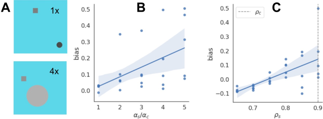
Figure 4: ResNet-18 prefers a shortcut feature when availability is instantiated as the pixel footprint of an object (feature), even when that feature is less predictive. A: Sample images. B: Shortcut bias increases as a function of relative availability of the shortcut feature when features are equally predictive ($\rho_{s}=\rho_{c}=0.9$), consistent with Wolff & Wolff (2022). C: Even when the shortcut feature is less predictive, models have a shortcut bias due to availability, when $\alpha_{s}/\alpha_{c}=4$.

Results. Figure 4B reports ResNet18 shortcut bias as a function of shortcut-feature availability (footprint) when the two features are equally predictive ($\rho_{s}=\rho_{c}=0.9$). In Figure 4C, the availability ratio is fixed at $\alpha_{s}/\alpha_{c}=4$, and the shortcut bias is assessed as a function of $\rho_{s}$. ResNet18 is biased toward the more available shortcut feature even when it is less predictive than the core feature. Together, these results suggest that a simple characteristic of image contents—the pixel footprint of an object—can bias models’ output behavior, and may therefore explain why models can fail to leverage typically-smaller foreground objects in favor of image backgrounds (Section 7).

6 Theoretical account

In our empirical investigations, we quantified the extent to which a trained model deviated from a statistically optimal classifier in its reliance on the more-available feature using a measure which considered the basis for probe-instance classifications. Here, we use an alternative approach of studying the sensitivity of a Neural Tangent Kernel (NTK) (Jacot et al., 2018) to the availability of a feature. The resulting form presents a crisp perspective of how predictivity and availability interact. In particular, we prove that availability bias is absent in linear networks but present in ReLU networks. The proof for the theorems of this section is presented in the Supplementary Materials.

For tractability of the analysis, we consider a few simplifying assumptions. We focus on 2-layer fully connected architectures for which the kernel of the ReLU networks admits a simple closed form. In addition, to be able to compute integrations that arise in the analysis, we resort to an asymptotic approximation which assumes covariance matrix is small. Specifically, we represent the covariance matrix as $s\,[\,1\,,\,\sigma_{12}\,;\,\sigma_{12}\,,\,1\,]$, where the scale parameter $s>0$ is considered to be small. Finally, in order to handle the analysis for ReLU kernel, we will use a polynomial approximation.

Kernel Spectrum. Consider a two-layer network with the first layer having a possibly nonlinear activation function. When the width of this model gets large, learning of this model can be approximated by a kernel regression problem, with a given kernel function $k(\,.\,,\,.\,)$ that depends on the architecture and the activation function. Given a distribution over the input data $p(\boldsymbol{x})$, we define a (linear) kernel operator as one that acts on a function $f$ to produce another function $g$ as in $g(\boldsymbol{x})\,=\,\int_{\mathbb{R}^{n}}k(\boldsymbol{x},\boldsymbol{z})\,f(\boldsymbol{z})\,p(\boldsymbol{z})\,d\boldsymbol{z}$. This allows us to define an eigenfunction $\phi$ of the kernel operator as one that satisfies,

$$\textstyle\lambda\,\phi(\boldsymbol{x})~{}=~{}\int_{\mathbb{R}^{n}}k(\boldsymbol{x},\boldsymbol{z})\,\phi(\boldsymbol{z})\,p(\boldsymbol{z})\,d\boldsymbol{z}\,.$$ (1)

The value of $\lambda$ will be the eigenvalue of that eigenfunction when the eigenfunction $\phi$ is normalized as

$\textstyle\int_{\mathbb{R}^{n}}\phi^{2}(\boldsymbol{x})\,p(\boldsymbol{x})\,d\boldsymbol{x}~{}=~{}1\,.$

Form of $p(\boldsymbol{z})$. Recall that in our generative dataset framework, we have a pair of latent features $z_{c}$ and $z_{s}$ that are embedded into a high dimensional space via $\textstyle\boldsymbol{x}_{\color[rgb]{1,0,0}d\times 1}\,=\,\alpha_{s}z_{s}\boldsymbol{w}_{s}+\alpha_{c}z_{c}\boldsymbol{w}_{c}\,=\,\boldsymbol{U}_{\color[rgb]{1,0,0}d\times 2}\boldsymbol{A}_{\color[rgb]{1,0,0}2\times 2}\boldsymbol{z}_{\color[rgb]{1,0,0}2\times 1}\,$. With this expression, we switch terminology such that our $\boldsymbol{w}_{i}\to\boldsymbol{U}$ and $\alpha_{i}\to\boldsymbol{A}$, and therefore $\boldsymbol{A}$ is diagonal matrix with positive diagonal entries, and the columns of $\boldsymbol{U}$ are (approximately) orthonormal. Henceforth, we also refer to features with indices 1 and 2 instead of $s$ and $c$. An implication of orthonormal columns on $\boldsymbol{U}$ is that the dot product of any two input vectors $\boldsymbol{x}$ and $\boldsymbol{x}^{\dagger}$ will be independent of $\boldsymbol{U}$, i.e., $\langle\boldsymbol{x},\boldsymbol{x}^{\dagger}\rangle\,=\,\langle\boldsymbol{A}\boldsymbol{z},\boldsymbol{A}\boldsymbol{z}^{\dagger}\rangle$. Consequently, we can compute dot products in the original 2-dimensional space instead of in the $d$-dimensional embedding space. On the other hand, we will later see that the kernel function $k(\boldsymbol{x}_{1},\boldsymbol{x}_{2})$ of the two cases we study here (ReLU and linear) depends on their input only through the dot product $\langle\boldsymbol{x}_{1},\boldsymbol{x}_{2}\rangle$ and norms $\|\boldsymbol{x}_{1}\|$ and $\|\boldsymbol{x}_{2}\|$ (self dot products). Thus, the kernel is entirely invariant to $\boldsymbol{U}$ and without loss of generality, we can consider the input to the model as $\boldsymbol{x}=\boldsymbol{A}\boldsymbol{z}$. Therefore,

$$\textstyle\boldsymbol{x}^{+}\sim\mathcal{N}\left(\begin{bmatrix}a_{1}\mu_{1}\\ a_{2}\mu_{2}\end{bmatrix},\begin{bmatrix}a_{1}^{2}&a_{1}a_{2}\sigma_{12}\\ a_{1}a_{2}\sigma_{12}&a_{2}^{2}\end{bmatrix}\right),~{}\boldsymbol{x}^{-}\sim\mathcal{N}\left(-\begin{bmatrix}a_{1}\mu_{1}\\ a_{2}\mu_{2}\end{bmatrix},\begin{bmatrix}a_{1}^{2}&a_{1}a_{2}\sigma_{12}\\ a_{1}a_{2}\sigma_{12}&a_{2}^{2}\end{bmatrix}\right).$$

Linear kernel function. If the activation function is linear, then the kernel function simply becomes a standard dot product,

$$k(\boldsymbol{x}_{1},\boldsymbol{x}_{2})\,\triangleq\,\left\langle\boldsymbol{x}_{1},\boldsymbol{x}_{2}\right\rangle\,.$$ (2)

The following theorem provides details about the spectrum of this kernel.

Theorem 1

Consider the kernel function $k(\boldsymbol{x}_{1},\boldsymbol{x}_{2})\,\triangleq\,\left\langle\boldsymbol{x}_{1},\boldsymbol{x}_{2}\right\rangle$. The kernel operator associated with $k$ under the data distribution $p$ specified above has only one non-zero eigenvalue $\lambda=\|\boldsymbol{A}\boldsymbol{\mu}\|^{2}$ and its eigenfunction has the form $\phi(\boldsymbol{x})\,=\,\frac{\langle\boldsymbol{A}\boldsymbol{\mu},\boldsymbol{x}\rangle}{\|\boldsymbol{A}\boldsymbol{\mu}\|^{2}}$.

ReLU kernel function. If the activation function is set to be a ReLU, then the kernel function is known to have the following form (Cho & Saul, 2009; Bietti & Bach, 2020):

$$k(\boldsymbol{x}_{1},\boldsymbol{x}_{2})\,\triangleq\,\|\boldsymbol{x}_{1}\|\,\|\boldsymbol{x}_{2}\|\,h\left(\left\langle\frac{\boldsymbol{x}_{1}}{\|\boldsymbol{x}_{1}\|},\frac{\boldsymbol{x}_{2}}{\|\boldsymbol{x}_{2}\|}\right\rangle\right)\,,~{}h(u)\,\triangleq\,\frac{1}{\pi}\Bigg{(}u\Big{(}\pi-\arccos(u)\Big{)}+\sqrt{1-u^{2}}\Bigg{)}\,.$$ (3)

In order to obtain an analytical form for the eigenfunctions of the kernel under the considered data distribution, we resort to a quadratic approximation of $h$ by $\widehat{h}$ as $\widehat{h}(u)\,\triangleq\,\frac{815}{3072}(1+u)^{2}$. This approximation enjoys certain optimality criteria. Derivation details of this quadratic form are provided in the Supplementary Materials, as is a plot showing the quality of the approximation. We now focus on spectral characteristics of the approximate ReLU kernel. Replacing $h$ in the kernel function $k$ of Equation 3 with $\widehat{h}$, we obtain an alternative kernel function approximation for ReLUs:

$$\vspace{-.1in}\textstyle{k}(\boldsymbol{x},\boldsymbol{z})\,\triangleq\,\|\boldsymbol{x}\|\,\|\boldsymbol{z}\|\,\widehat{h}\left(\left\langle\frac{\boldsymbol{x}}{\|\boldsymbol{x}\|},\frac{\boldsymbol{z}}{\|\boldsymbol{z}\|}\right\rangle\right)\,=\,\|\boldsymbol{x}\|\,\|\boldsymbol{z}\|\,a^{*}\left(1+\left\langle\frac{\boldsymbol{x}}{\|\boldsymbol{x}\|},\frac{\boldsymbol{z}}{\|\boldsymbol{z}\|}\right\rangle\right)^{2}\,.$$ (4)

The following theorem characterizes the spectrum of this kernel.

Theorem 2

Consider the kernel function $\textstyle k(\boldsymbol{x},\boldsymbol{z})\,\triangleq\,\|\boldsymbol{x}\|\,\|\boldsymbol{z}\|\,a^{*}\left(1+\left\langle\frac{\boldsymbol{x}}{\|\boldsymbol{x}\|},\frac{\boldsymbol{z}}{\|\boldsymbol{z}\|}\right\rangle\right)^{2}$. The kernel operator associated with $k$ under the data distribution $p$ specified above has only two non-zero eigenvalues $\lambda_{1}=\lambda_{2}=2a^{*}\|\boldsymbol{A\mu}\|^{2}$ with associated eigenfunctions given by

$$\textstyle\phi_{1}(\boldsymbol{x})\,=\,\frac{\|\boldsymbol{x}\|}{\|\boldsymbol{A}\boldsymbol{\mu}\|}\frac{1+\left\langle\frac{\boldsymbol{x}}{\|\boldsymbol{x}\|},\frac{\boldsymbol{A}\boldsymbol{\mu}}{\|\boldsymbol{A}\boldsymbol{\mu}\|}\right\rangle^{2}}{2}\textrm{~{}~{}and~{}~{}}\phi_{2}(\boldsymbol{x})\,=\,\left\langle\frac{\boldsymbol{x}}{\|\boldsymbol{A}\boldsymbol{\mu}\|},\frac{\boldsymbol{A}\boldsymbol{\mu}}{\|\boldsymbol{A}\boldsymbol{\mu}\|}\right\rangle.$$

6.1 Sensitivity Analysis

We now assign a target value $y(\boldsymbol{x})$ to each input point $\boldsymbol{x}$. Under the squared loss for regression. By expressing the kernel operator using its eigenfunctions, it is easy to show that $f(\boldsymbol{x})\,=\,\sum_{i}(\phi_{i}(\boldsymbol{x})\int_{\mathbb{R}^{n}}\phi_{i}(\boldsymbol{z})\,y(\boldsymbol{z})\,p(\boldsymbol{z})\,d\boldsymbol{z})$ where $i$ runs over non-zero eigenvalues $\lambda_{i}$ of the kernel operator (see also Appendix G). We now restrict our focus to a binary classification scenario, $y:\mathcal{X}\rightarrow\{0,1\}$. More precisely, we replace $p$ with our Gaussian mixture and set $y(\boldsymbol{x})$ to 1 and 0 depending on whether $\boldsymbol{x}$ is drawn from the positive or negative component of the mixture.

$$\textstyle f(\boldsymbol{x})\,=\,\sum_{i}\Big{(}\phi_{i}(\boldsymbol{x})\big{(}\frac{1}{2}\int_{\mathbb{R}^{2}}\phi_{i}(\boldsymbol{z})\,(1)\,p^{+}(\boldsymbol{z})\,d\boldsymbol{z}+\frac{1}{2}\int_{\mathbb{R}^{2}}\phi_{i}(\boldsymbol{z})\,(0)\,p^{-}(\boldsymbol{z})\,d\boldsymbol{z}\big{)}\Big{)}\,=\,\frac{1}{2}\sum_{i}\phi_{i}(\boldsymbol{x})\phi_{i}(\boldsymbol{A}\boldsymbol{\mu})\,,$$

where $p^{+}$ and $p^{-}$ denote class-conditional normal distributions. Now let us tweak the availability of each feature by a diagonal scaling matrix $\boldsymbol{B}\triangleq\operatorname{diag}(\boldsymbol{b})$ where $\boldsymbol{b}\triangleq[b_{1},b_{2}]$. Denote the modified prediction function as $g_{\boldsymbol{B}}$. That is, $g_{\boldsymbol{B}}(\boldsymbol{x})\,\triangleq\,\frac{1}{2}\sum_{i}\phi_{i}(\boldsymbol{x})\phi_{i}(\boldsymbol{B}\boldsymbol{A}\boldsymbol{\mu})$. The alignment between $f$ and $g$ is their normalized dot product,

$$\textstyle\gamma(\boldsymbol{b})\,\triangleq\,\int_{\mathbb{R}^{2}}\frac{f(\boldsymbol{x})}{\sqrt{\int_{\mathbb{R}^{2}}f^{2}(\boldsymbol{t})p(\boldsymbol{t})\,d\boldsymbol{t}}}\frac{g_{\boldsymbol{B}}(\boldsymbol{x})}{\sqrt{\int_{\mathbb{R}^{2}}g_{\boldsymbol{B}}^{2}(\boldsymbol{t})p(\boldsymbol{t})\,d\boldsymbol{t}}}p(\boldsymbol{x})\,d\boldsymbol{x}\,.$$ (5)

We define the sensitivity of the alignment to feature $i$ for $i=1,2$ as its $m$’th order derivative of $\gamma$ w.r.t. $b_{i}$ evaluated at $\boldsymbol{b}=\boldsymbol{1}$ (which leads to identity scale factor $\boldsymbol{B}=\boldsymbol{I}$),

$$\small\textstyle\zeta_{i}\,\triangleq\,\Big{(}\frac{\partial^{m}}{\partial b_{i}^{m}}\,\gamma\Big{)}_{\boldsymbol{b}=\boldsymbol{1}}\,=\,\Big{(}\frac{\partial^{m}}{\partial b_{i}^{m}}\,\int_{\mathbb{R}^{2}}\frac{\sum_{i}\phi_{i}(\boldsymbol{x})\phi_{i}(\boldsymbol{A}\boldsymbol{\mu})}{\sqrt{\int_{\mathbb{R}^{2}}\big{(}\sum_{i}\phi_{i}(\boldsymbol{x})\phi_{i}(\boldsymbol{A}\boldsymbol{\mu})\big{)}^{2}\,d\boldsymbol{t}}}\,\frac{\sum_{i}\phi_{i}(\boldsymbol{x})\phi_{i}(\boldsymbol{B}\boldsymbol{A}\boldsymbol{\mu})}{\sqrt{\int_{\mathbb{R}^{2}}\big{(}\sum_{i}\phi_{i}(\boldsymbol{x})\phi_{i}(\boldsymbol{B}\boldsymbol{A}\boldsymbol{\mu})\big{)}^{2}\,d\boldsymbol{t}}}\,d\boldsymbol{x}\Big{)}_{\boldsymbol{b}=\boldsymbol{1}}\,.$$

$\zeta_{i}$ indicates how much the model relies on feature $i$ to make a prediction. In particular, if whenever feature $i$ is more available than feature $j$, i.e. $a_{i}>a_{j}$, we also see the model is more sensitive to feature $i$ than feature $j$, i.e. $|\zeta_{i}|>|\zeta_{j}|$, the model is biased toward the more-available feature. In addition, when $a_{i}<a_{j}$ but $|\zeta_{i}|>|\zeta_{j}|$, the bias is toward the less-available feature. One can express the presence of these biases more concisely as $\textstyle\operatorname{sign}\Big{(}(|\zeta_{1}|-|\zeta_{2}|)(a_{1}-a_{2})\Big{)}$, where values of $+1$ and $-1$ indicate bias toward more- and less- available features, respectively. To verify either of these two cases via sensitivity, we must choose the lowest order $m$ that yields a non-zero $|\zeta_{1}|-|\zeta_{2}|$. On the other hand, if $|\zeta_{1}|-|\zeta_{2}|=0$ for any choice of $a_{1}$ and $a_{2}$, the model is unbiased to feature availability.

The following theorems now show that linear networks are unbiased to feature availability, while ReLU networks are biased toward more available features.

Theorem 3

In a linear network, $|\zeta_{1}|-|\zeta_{2}|$ is always zero for any choice of $m\geq 1$ and regardless of the values of $a_{1}$ and $a_{2}$.

Theorem 4

In a ReLU network, $|\zeta_{1}|-|\zeta_{2}|=0$ for any $1\leq m\leq 8$. The first non-zero $|\zeta_{1}|-|\zeta_{2}|$ happens at $m=9$ and has the following form,

$$|\zeta_{1}|-|\zeta_{2}|\,=\,\frac{5670}{\|\boldsymbol{A}\boldsymbol{\mu}\|^{18}}(a_{1}a_{2}\mu_{1}\mu_{2})^{8}(a_{1}^{2}\mu_{1}^{2}-a_{2}^{2}\mu_{2}^{2})\,.$$ (6)

A straightforward consequence of this theorem is that

$$\operatorname{sign}\Big{(}(|\zeta_{1}|-|\zeta_{2}|)(a_{1}-a_{2})\Big{)}\,=\,\operatorname{sign}\Big{(}\frac{5670}{\|\boldsymbol{A}\boldsymbol{\mu}\|^{18}}(a_{1}a_{2}\mu_{1}\mu_{2})^{8}(a_{1}^{2}\mu_{1}^{2}-a_{2}^{2}\mu_{2}^{2})(a_{1}-a_{2})\Big{)}\,=\,\operatorname{sign}\Big{(}(a_{1}^{2}\mu_{1}^{2}-a_{2}^{2}\mu_{2}^{2})(a_{1}-a_{2})\Big{)}\,.$$ (7)

Recall from Section 3 that feature predictivity $\rho_{i}$ is related to $\mu_{i}$ via $\rho_{i}=\frac{1}{2}(1+\mathrm{erf}(\frac{\mu_{i}}{\sqrt{2}}))$. Observe that $\rho_{i}$ is an increasing function in $\mu_{i}$; bigger $\mu_{i}$ implies larger $\rho_{i}$. Putting that beside (7) provides a crisp interpretation of the trade-off between predictivity and availability. For example, when the latent features are equally predictive ($\mu_{1}=\mu_{2}$), the $\operatorname{sign}$ becomes $+1$ for any (non-negative) choice of availability parameters $a_{1}$ and $a_{2}$. Thus, for equally predictive features, the ReLU networks are always biased toward the more available feature. Figure 5 shows some more examples with certain levels of predictivity. The coloring indicates the direction of the availability bias (only the boundaries between the blue and the yellow regions have no availability bias).

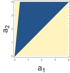
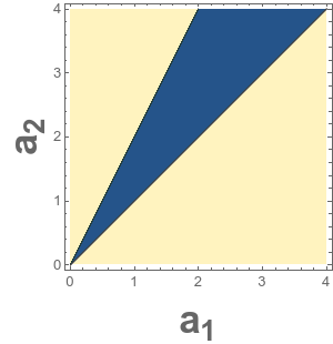
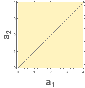
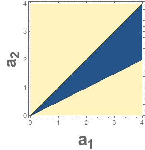
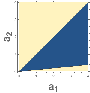
$\small\mu_{2}=0.1$	$\small\mu_{2}=0.5$	$\small\mu_{2}=1$	$\small\mu_{2}=2$	$\small\mu_{2}=10$

Figure 5: Plot of $\operatorname{sign}((|\zeta_{1}|-|\zeta_{2}|)(a_{1}-a_{2}))$ for ReLU network as a function of $a_{1}$ and $a_{2}$. We fix $\mu_{1}=1$ and vary $\mu_{2}\in\{0.1,0.5,1,2,10\}$. Yellow and blue correspond to values $+1$ and $-1$ respectively.

7 Feature availability in naturalistic datasets

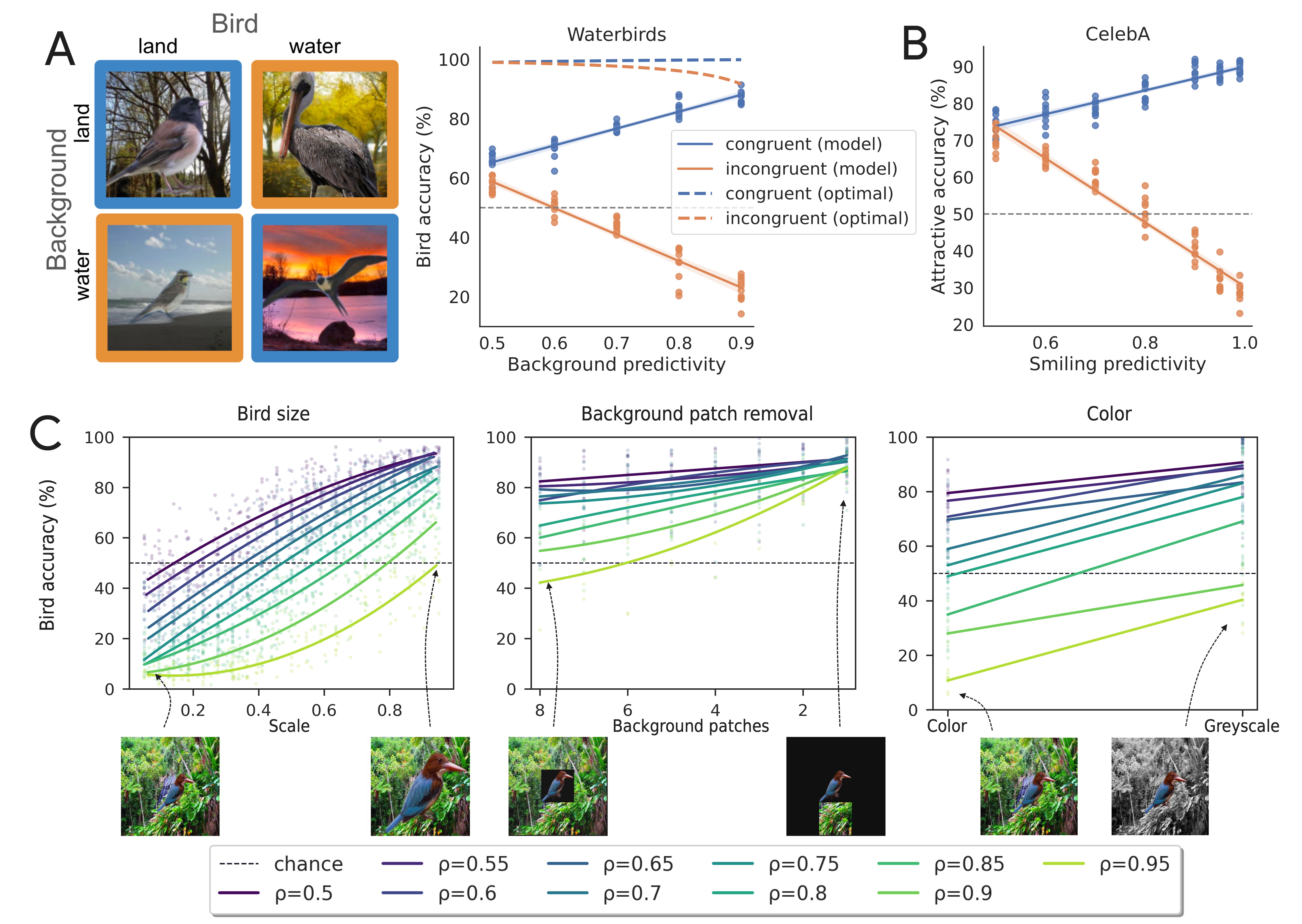
Figure 6: Availability as well as predictivity determines which features image classifiers rely on. A: Models (ResNet18) were trained to classify Birds from images sampled from Waterbirds. We varied Background (non-core) predictivity while keeping Bird (core) predictivity fixed ($=0.99$), and show Bird classification accuracy for two types of probes: congruent (blue, core and non-core features support the same label) and incongruent (orange, core and non-core features support opposing labels). As Background predictivity increases, the gap in accuracy between incongruent and congruent probes also increases. The model is more sensitive to the non-core feature than expected by a Bayes-optimal classifier (optimal): predictivity alone does not explain the model’s behavior. B: Similar to the Waterbirds dataset, models trained to classify images from CelebA as “Attractive” exhibit an effect of “Smiling” availability. C: Bird accuracy for incongruent Waterbirds probes is influenced by both Background predictivity ($\rho$) and availability when we manipulate the latter explicitly (see also B.9).

We have seen that models trained on controlled, synthetic data are influenced by availability to learn shortcuts when a nonlinear activation function is present. How do feature predictivity and availability in naturalistic datasets interact to shape the behavior of models used in practice? To test this, we train ResNet18 models (He et al., 2016) to classify naturalistic images by a binary core feature irrespective of the value of a non-core feature. We construct two datasets by sampling images from Waterbirds (Sagawa et al., 2020a) (core: Bird, non-core: Background), and CelebA (Liu et al., 2015) (core: Attractive, non-core: Smiling). See C.5 for additional details.

Sensitivity to the non-core feature beyond a statistical account. Figures 6A and B show that, for both datasets, as the training-set predictivity of the non-core feature increases, model accuracy increases for congruent probes, but decreases for incongruent ones, whereas a Bayes optimal classifier is not comparably sensitive to the predictivity of the non-core feature. So, the model is more influenced by the non-core feature than what we would expected based solely on predictivity. This heightened sensitivity implies that models prioritize the non-core feature more than they should, given its predictive value. Thus, in the absence of predictivity as an explanatory factor, we conclude that the non-core feature is more available than the core feature.

Availability manipulations. Motivated by the result that Background is more available to models than the core Bird (Figure 6A), we test whether specific background manipulations (hypothesized types of availability) shift model feature reliance. As shown in Figure 6C, we find that Bird accuracy increases as we reduce the availability of the image background by manipulating its spatial extent (Bird size, Background patch removal) or drop background color (Color), implicating these as among the features that models latch onto in preferring image backgrounds (validated with explainability analyses in C.5). Experiments in Figure B.9 show that this phenomenon also occurs in ImageNet-pretrained models; background noise and spatial frequency manipulations also drive feature reliance.

8 Conclusion

Shortcut learning is of both scientific and practical interest given its implications for how models generalize. Why do some features become shortcut features? Here, we introduced the notion of availability and conducted studies systematically varying availability. We proposed a generative framework that allows for independent manipulation of predictivity and availability of latent features. Testing hypotheses about the contributions of each to model behavior, we find that for both vector and image classification tasks, deep nonlinear models exhibit a shortcut bias, deviating from the statistically optimal classifier in their feature reliance. We provided a theoretical account which indicates the inevitability of a shortcut bias for a single-hidden-layer nonlinear (ReLU) MLP but not a linear one. The theory specifies the exact interaction between predictivity and availability, and consistent with our empirical studies, predicts that availability can trump predictivity. In naturalistic datasets, vision architectures used in practice rely on non-core features more than they should on statistical grounds alone. Connecting with prior work identifying availability biases for texture and image background, we explicitly manipulated background properties such as spatial extent, color, and spatial frequency and found that they influence a model’s propensity to learn shortcuts.

Taken together, our empirical and theoretical findings highlight that models used in practice are prone to shortcut learning, and that to understand model behavior, one must consider the contributions of both feature predictivity and availability. Future work will study shortcut features in additional domains, and develop methods for automatically discovering further shortcut features which drive model behavior. The generative framework we have laid out will support a systematic investigation of architectural manipulations which may influence shortcut learning.

Supplementary Material for
“On the Foundations of Shortcut Learning”

Appendix A Broader impacts

Our work aims to achieve a principled and fundamental understanding of the mechanisms of deep learning—when it succeeds, when it fails, and why it fails. As the goal is to better understand existing algorithms, there is no downside risk of the research. The upside benefit concerns cases of shortcut learning which have been identified as socially problematic and where fairness issues are at play, for example, the use of shortcut features such as gender or ethnicity that might be spuriously correlated with a core feature (e.g., likelihood of default).

Appendix B Supplementary figures

Methods details accompanying these figures appear in Section C.

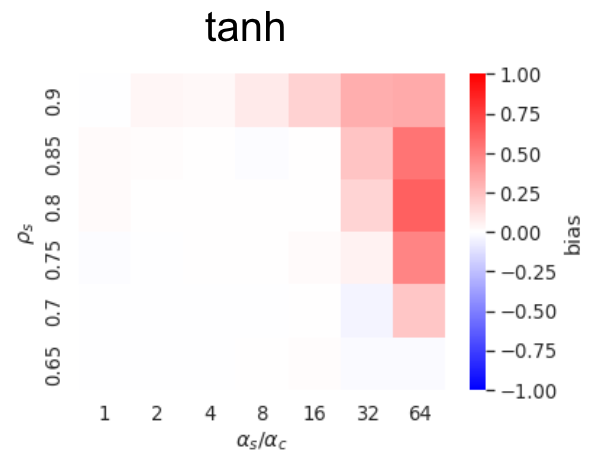
Figure B.1: Bias as a function of $z_{s}$ availability and predictivity for a single-hidden-layer MLP with a $\mathrm{tanh}$ hidden-layer activation function. Settings match those described in Figure 3C.

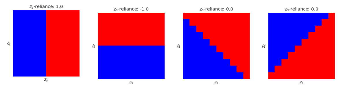
Figure B.2: The $z_{s}$-reliance (Sections 3 and C.1) of hypothetical classifiers which rely exclusively on $z_{s}$ (top left) or $z_{c}$ (top right), or rely equally on both features (bottom row). Color indicates the predicted label (red: pos, blue: neg) for probe items plotted by base probe ($z_{s}$, $z_{c}$) values

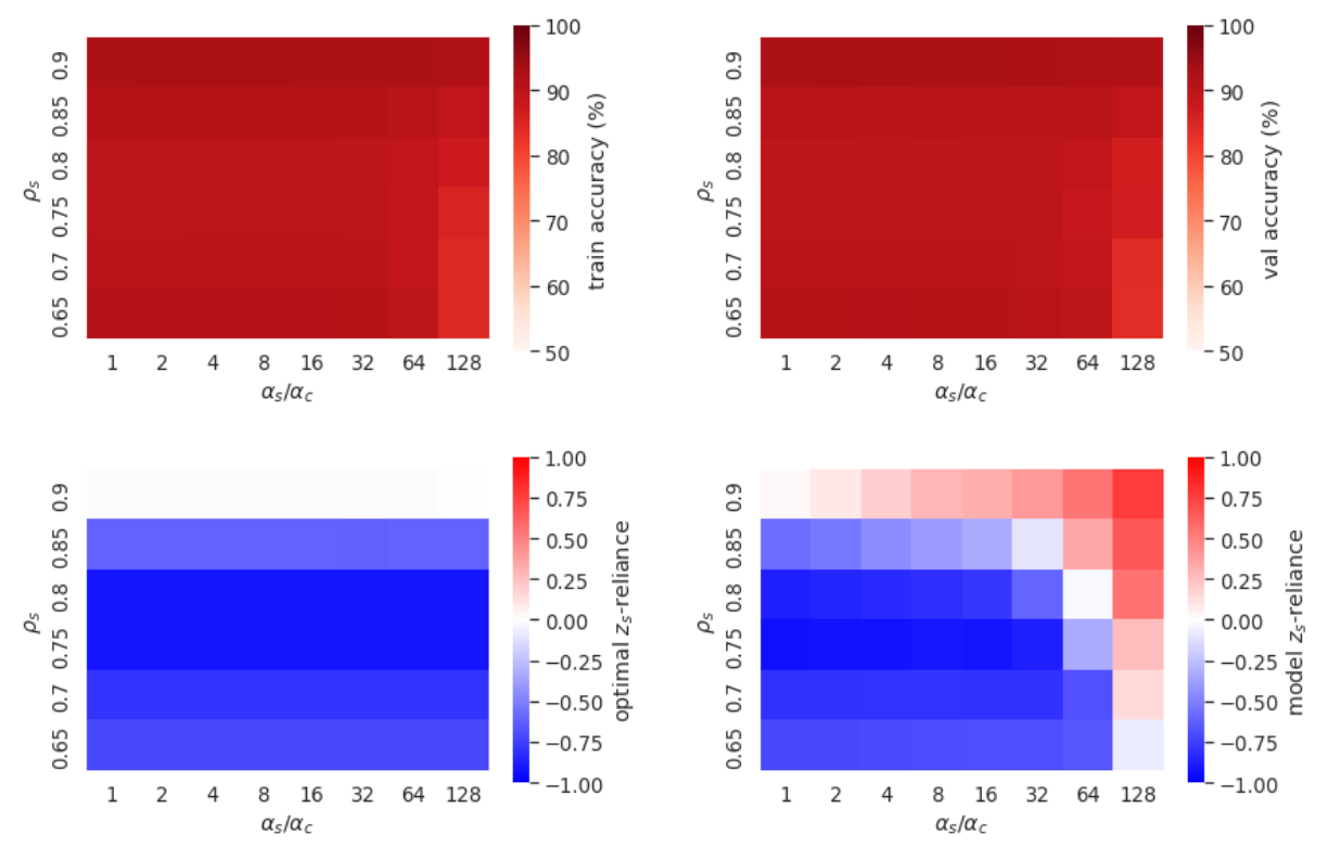
Figure B.3: Supplementary data for the results presented in Figure 2. Top row: Model performance on the train (left) and validation (right) sets. Bottom row: $z_{s}$-reliance for the optimal classifier (left) and models (right).

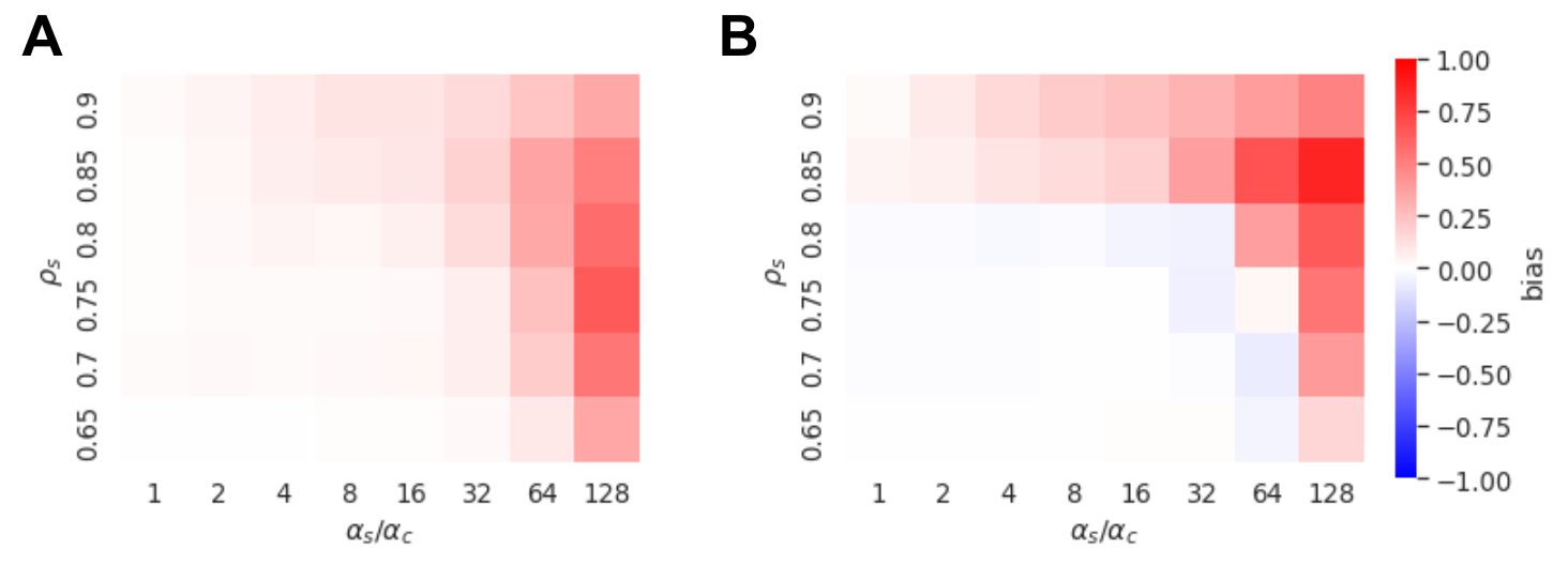
Figure B.4: The results shown in Figure 2 are not specific to choice of $\sigma_{sc}$. Results for the same experiment using datasets with $\sigma_{sc}=0.4$ (A) and $\sigma_{sc}=0.8$ (B).

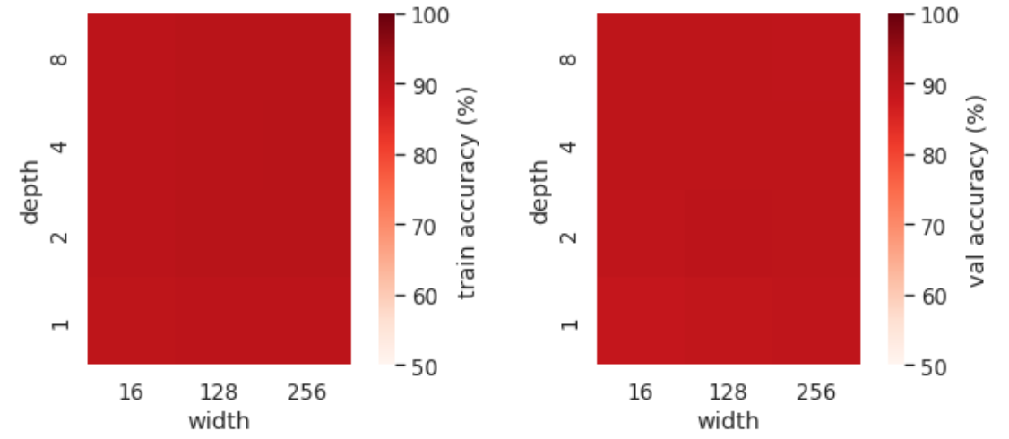
Figure B.5: Supplementary data for the results presented in Figure 3. Model performance on the train (left) and validation (right) sets.

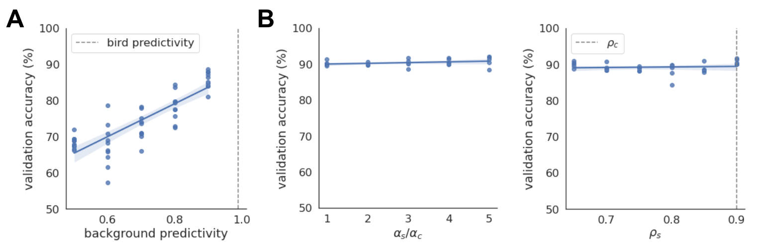
Figure B.6: Supplementary data for image experiments. Model performance underlying A: Experiments with the Waterbirds datasets presented in Figure 6 and described in C.5, and B: Experiments with image instantiations of the base dataset manipulating pixel footprint presented in Figure 4 B (left) and C (right).

Figure B.7: Models prefer a shallowly embedded nonlinear feature ($z_{s}$) to a deeply embedded nonlinear one ($z_{c}$). A: The color of each cell of the heatmap indicates the mean bias of models as a function of the degree of nesting of $z_{c}$ ($\eta_{c}$), and the predictivity of $z_{s}$ ($\rho_{s}$). $z_{s}$ is always shallowly embedded ($\eta_{s}=0$), and the predictivity of $z_{c}$ is held fixed ($\rho_{c}=0.9$). See C.3 for additional details. B: Model performance. C:$z_{s}$-reliance of the optimal classifier (left) versus the model (right).

Figure B.8: Illustration of studied Background availability manipulations. For each of the six perturbations influencing the availability of both the background and the bird (in the case of bird scale), we provide visual representations of the potential perturbations applied to the training dataset. For instance, the first row demonstrates variations in the dataset resulting from changes in bird size, ranging from 5% to 95%.

Figure B.9: Manipulations of image backgrounds show that availability as well as predictivity determines feature reliance in vision models, including in models pretrained on ImageNet. Expanding on the results shown in Figure 6, we plot Bird accuracy for incongruent probes (opposing Bird and Background labels) as a function of Background predictivity ($\rho$) and hypothesized types of availability. Top row: ResNet18 models. Bottom row: IN ResNet50 models (see Section C.5 for additional details).

Figure B.10: Explainability sanity check: Attribution maps corroborate Background availability study. In Figures 6 and B.9, we saw that a Bird size manipulation affects models’ tendency to classify incongruent probes consistent with their Bird labels. Here, we see that attribution maps for probe images (top row) reflect a difference in focal point for models trained on images with Bird size $=40\%$ (preference for image background) versus Bird size $=80\%$ (preference for foreground bird). See C.5 for additional details.

Appendix C Supplementary methods and results

C.1 Assessing bias

In Section 3, we described how we determine $\textit{reliance}_{\mathcal{M}}$, a score which quantifies the extent to which a model (optimal classifier or trained model) uses feature $z_{s}$ as the basis for its classification decisions. In Figure B.2, for intuition, we show the $z_{s}$ reliance of hypothetical classifiers.

C.2 Synthetic data

Optimal classifier. To obtain optimal classifications, we use Linear Discriminant Analysis (LDA, as implemented in Sklearn with the least-squares solver). In all but the experiments on the effect of nesting as part of the generative process (C.3 and Figure B.7), the optimal classifier was fit to and probed with the same embedded base inputs used to train the corresponding model in a given experiment. In the nesting experiments, LDA was fit to and probed with base inputs directly.

C.3 Vector experiments

Default model architecture and training procedure. Unless otherwise described, we train a multi-layer perceptron (MLP, depth $=8$, width $=128$, hidden activation function $=$ ReLU) with MSE loss for 100 epochs using an SGD optimizer with batch size $=64$ and learning rate $=1e-02$. We use Glorot Normal weight initialization.

Models prefer the more-available feature, even when it is less predictive. In these experiments, given a base dataset with ($\rho_{s},\rho_{c}$), for each availability setting ($\alpha_{s},\alpha_{c}$), we manipulate the availability of the dataset, sample a random intialization seed, train the default model architecture, and evaluate the bias of the model. We repeat this process for each of $10$ runs, computing the biases for individual (model, optimal classifier) pairs, and then averaging the results.

Effect of nesting on availability. Figure 1B illustrates how our generative procedure for synthetic datasets supports nested embedding of latent features, as described in Section 3. In this experiment, we test whether a model prefers a shallowly embedded nonlinear feature ($z_{s}$) to a deeply embedded nonlinear one ($z_{c}$) when the amplitude of both features is matched ($\alpha_{s}=\alpha_{c}=0.1$) and the nonlinearity is a scaled $\mathrm{tanh}$ ($\mathrm{tanh}(\lambda x)$, with $\lambda=100$). After embedding each feature as $\boldsymbol{e}_{i}=\alpha_{i}\boldsymbol{w}_{i}z_{i}$, we apply the nonlinearity. For a nesting factor $\eta_{i}>0$, we pass $e_{i}$ through a fully connected network (depth = $\eta_{i}$, width $=d$, no bias weights) with scaled $\mathrm{tanh}$ activations on the hidden and output layers. We initialize weight matrices to be random special orthogonal matrices (implemented as scipy.stats.special_ortho_group). In Figure B.7, we show bias as a function of $\eta_{c}$ and $\rho_{s}$; $z_{s}$ is fixed to be shallowly embedded with $\eta_{s}=0$ and has $\rho_{c}=0.9$. We report the results as the mean across 3 runs.

C.4 Pixel footprint experiments

Model architecture and training procedure. In these experiments, we train a randomly initialized ResNet18 architecture with MSE loss using an Adam optimizer with batch size $=64$ and learning rate $=1e-02$, taking the best (defined on validation accuracy) across 100 epochs of training. For each ($\rho_{s},\rho_{c}$) predictivity setting, we repeat this process for 10 (sampled dataset, random weight initialization) runs.

Analyses. In Figure 4, we report results for experiments in which we use a base $z_{s}$ pixel footprint of $400$ px, and manipulate $z_{s}$ pixel footprint to be $1-5\times$ larger ($\alpha_{c}=1$, $\alpha_{s}\in[1,5]$). To determine the bias of a model, we compute the $z_{s}$-reliance of the trained model given image instantiations of the base probe items, and compare to the $z_{s}$-reliance of the optimal classifier (LDA) fit to and probed using vector instantiations of the same base dataset with the same $\alpha_{s}$ and $\alpha_{c}$. We repeat this process for 5 runs, computing bias on a per-run basis as in Section C.3.

C.5 Feature availability in naturalistic datasets

Datasets. Waterbirds. Waterbirds images (Sagawa et al., 2020a) combine birds taken from the Caltech-UCSD Birds-200-2011 dataset (Wah et al., 2011) and backgrounds from the Places dataset (Zhou et al., 2017). To construct the datasets used in Figure 6A, we sample images from a base Waterbirds dataset generated using code by (Sagawa et al., 2020a) (github.com/kohpangwei/group_DRO) with $\texttt{val frac}=0.2$ and $\texttt{confounder strength}=0.5$, yielding sets of $5694$ train images ($224\times 224$), $300$ validation images, and $5794$ test images. We then subsample these sets to $1200$ train, $90$ validation ($\times 2$ sets), and $1000$ probe images ($\times 2$ sets), respectively, such that the train and validation sets instantiate target feature predictivities, and the probe sets contain congruent or incongruent feature-values, as described in Section 7.

To construct the datasets used in Figures 6C and B.9, for a given predictivity setting, we subsample 8 bird types per category (land, water) and cross them with land and water backgrounds randomly sampled from the standard Waterbirds background classes, to generate class-balanced train sets ranging in size from $800-1200$, and incongruent probe sets of size $400$.

CelebA. The CelebA (Liu et al., 2015) dataset contains images of celebrity faces paired with a variety of binary attribute labels. In our experiments, we cast the “Attractive” label as the core feature, and the “Smiling” label as the non-core feature. To construct the datasets used in Figure 6B, we sample images consistent with the target predictivities.

Waterbirds availability manipulations. In the datasets depicted in Figures 6C and B.9, we aim to manipulate various aspects of background availability. To do so, we use CUB-200 masks to exclusively modify the background, and apply five distinct types of perturbations: altering bird size, removing background patches, changing background colors, applying low-pass filtering, adding Perlin noise, and adding white noise. These perturbations test hypotheses about specific image properties than may make an image background more available to a model than the foreground object. We vary Background predicitivity while holding bird predictivity fixed ($=0.99$). We report results for at least 500 runs (model training) for each perturbation type. Figure B.8 shows sample image to which the perturbations have been applied. In detail, the perturbations are as follow:

• Bird size: We manipulate the pixel footprint of the bird by scaling the square mask. Note that an increase in bird size corresponds to a decrease in background pixels in the image.

• Background patch removal: This manipulation removes patches of the image background while preserving the foreground bird. To apply the manipulation, we partition the image into a $3\times 3$ checkerboard, position the bird in the center, and then remove $x$ in $[1,8]$ background cells.

• Color: To assess the influence of color information, we use the original image with its colored background (“Color”) or convert the background to grayscale (“Grayscale”).

• Low-pass filtering: We apply a low-pass filter to the frequency representation of the background, with the cutoff frequency varying from 224 (original image) to 2 (retaining only components at 2 cycles per image).

• Uniform noise: Uniform noise is introduced to the image with an amplitude ranging from 0 (original image) to 255. It is essential to note that image values are clipped within the (0, 255) range before preprocessing.

• Perlin noise: We apply Perlin noise, which possesses spatial coherence, at various intensity levels along with uniform noise. We employ 6-octave Perlin noise to match the frequency distribution of natural backgrounds (wavelengths 2, 4, 8, 16, 32, 64, and 128).

Model architecture and training procedure. For the experiments shown in Figure 6A and B, we normalize all images by the ImageNet train-set statistics (RGB mean $=[0.485,0.456,0.406]$), std $=[0.229,0.224,0.225]$), and then use the same settings as described in 5.

In the experiments shown in Figures 6C and B.9, we preprocess images by normalizing to be in $[-1,1]$, apply random crops of size $200\mid 200$, resize to $224\mid 224$, and randomly flip over the horizontal axis with $p=0.5$ We train models with MSE loss using an Adam optimizer with batch size $=32$, cosine decay learning rate schedule (linear warmup, initial learning rate $=1e-03$), and weight decay $=1e-05$. For the ResNet18 experiments in Figures 6C and B.9, we train a randomly initialized ResNet18 trained for 30 epochs. For the ResNet50 experiments in Figure B.9, we train the randomly initialized readout layer of a frozen, ImageNet-pretrained ResNet50 (IN ResNet50) for 15 epochs.

Results: Vision models, including ImageNet-pretrained ones, are sensitive to Background availability manipulations. Figure B.9 displays the results of the six manipulations which we hypothesized affect Background availability. The top row shows accuracy for ResNet18 models trained from scratch, while the bottom row shows the results for IN-ResNet50. Our findings reveal several key observations:

First, as the size of the bird increases (Col.1), as well as when the background becomes noisier (Col. 4,6), filtered of its high frequencies (Col 5), or simply masked (Col 2), the model tends to rely more heavily on the bird itself for classification. Conversely, when the background is clear and informative (available), the model utilizes the background features to predict the class. Second, the spuriousness of the background, as quantified by $\rho$, also has a discernible effect on the model’s behavior. However, it only partially accounts for the observed variations, demonstrating that availability factors are at play. Last, these results indicate that pretraining has a beneficial impact and can modulate feature availability. This effect may be attributed to the learned invariances during the pretraining process, enabling the model to better adapt to different availability conditions. Our spatial frequency experiments complement existing and concurrent work studying what models learn as a function of spatial frequency manipulations at training (Jo & Bengio, 2017; Yin et al., 2019; Tsuzuku & Sato, 2019; Hermann et al., 2020; Subramanian et al., 2023) or test time (Geirhos et al., 2018b).

Results: Explainability analyses corroborate Background availability study. The experiments presented in Figures 6C and B.9 showed that the degree of Background availability influences model classifications of incongruent probes. Here, we use attribution methods to verify that when a model predominantly relies on the image background, or on the foreground bird, according to the experimental results, its focal point reflect this. Figure B.10 shows the attributions maps of two ResNet18 models trained from scratch, one using a bird size of 40%, and the other using a bird size of 80%. For the same set of probe images, the model trained on larger birds exhibits a strategy shift in classification, seemingly having his focal point on the birds, whereas the model trained on smaller birds mainly relies on the background. The methods employed encompass a combination of black-box techniques (Rise (Petsiuk et al., 2018) and Sobol indices (Fel et al., 2021)) and gradient-based approaches (Saliency (Zeiler & Fergus, 2014) and Smoothgrad (Smilkov et al., 2017)).

Appendix D Quadratic Approximation of h

Since $u$ is the dot product of two normalized vectors, its range is limited to $-1\leq u\leq 1$. Observe that the derivative of $h$ has the form,

$$h^{\prime}(u)\,=\,1-\frac{1}{\pi}\arccos(u)\,.$$ (8)

The only place within $u\in[-1,1]$ that $h^{\prime}$ vanishes is at $u=-1$, suggesting the critical point of our quadratic must lie at this point. Furthermore, observe that $h(-1)=0$. Forcing these two constraints onto our quadratic, leaves us with the form,

$$\widehat{h}(u)\,=\,a(1+u)^{2}\,,$$ (9)

where $a$ is a parameter to be determined. Our aim is to find $a$ so that the function $\widehat{h}$ and $h$ looks similar over the entire domain $u\in[-1,1]$. We choose $\ell_{2}$ error between the two functions defined as,

$$e_{a}=\int_{-1}^{1}\Big{(}h(u)-\widehat{h}(u)\Big{)}^{2}d\,u\,.$$ (10)

Replacing the definitions for $h$ and $\widehat{h}$ into $(h(u)-\widehat{h}(u))^{2}$, one can obtain

$$e_{a}=\frac{1}{3}-\frac{163}{48}a+\frac{32}{5}a^{2}+\frac{32}{27\pi^{2}}\,.$$ (18)

Since $e_{a}$ is a convex quadratic in $a$, its minimizer can be determined by zero-crossing the derivative of $e_{a}$ w.r.t. $a$. This yields,

$$a^{*}\,\triangleq\,\arg\min_{a}e_{a}\,=\,\frac{815}{3072}\,.$$ (19)

This leads to the claimed quadratic form,

$$\widehat{h}(u)\,\triangleq\,\frac{815}{3072}(1+u)^{2}\,.$$ (20)

Figure D.1 shows a plot of the original $h$ and the quadratic approximation $\widehat{h}$ to visually get a sense of the approximation quality.

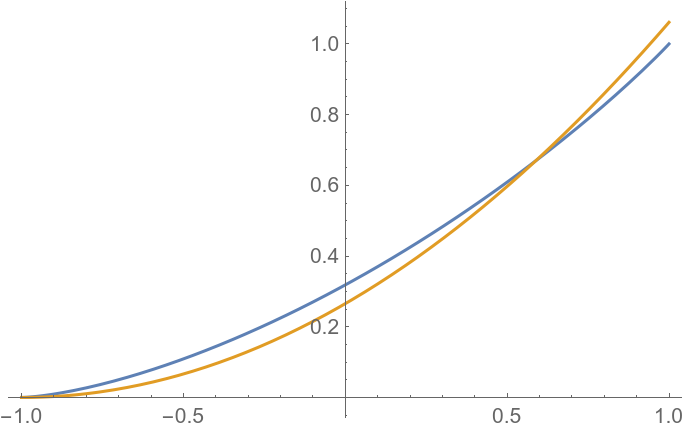
Figure D.1: The plots for $h$ (blue) $\widehat{h}$ (orange) within $u\in[-1,1]$.

Appendix E Proof of ReLU Kernel Theorem

Recall that the kernel function $k$ for ReLU is expressed using $h$ as in (3). Replacing $h$ with $\widehat{h}$ thus gets us an alternate kernel function which approximates that of ReLU’s.

$${k}(\boldsymbol{x},\boldsymbol{z})\,\triangleq\,\|\boldsymbol{x}\|\,\|\boldsymbol{z}\|\,\widehat{h}\left(\left\langle\frac{\boldsymbol{x}}{\|\boldsymbol{x}\|},\frac{\boldsymbol{z}}{\|\boldsymbol{z}\|}\right\rangle\right)\,=\,\|\boldsymbol{x}\|\,\|\boldsymbol{z}\|\,a^{*}\left(1+\left(\left\langle\frac{\boldsymbol{x}}{\|\boldsymbol{x}\|},\frac{\boldsymbol{z}}{\|\boldsymbol{z}\|}\right\rangle\right)\right)^{2}\,.$$ (21)

E.1 Eigenfunctions

An eigenfunction $\phi$ must satisfy,

$$\int_{\mathbb{R}^{n}}a^{*}\,\|\boldsymbol{x}\|\,\|\boldsymbol{z}\|\,\left(1+\left\langle\frac{\boldsymbol{x}}{\|\boldsymbol{x}\|},\frac{\boldsymbol{z}}{\|\boldsymbol{z}\|}\right\rangle\right)^{2}\,\phi(\boldsymbol{z})p(\boldsymbol{z})\,d\boldsymbol{z}\quad=\quad\lambda\,\phi(\boldsymbol{x})\,,$$ (22)

or equivalently,

$$a^{*}\,\|\boldsymbol{x}\|\,\int_{\mathbb{R}^{n}}\|\boldsymbol{z}\|\,\left(1+\left\langle\frac{\boldsymbol{x}}{\|\boldsymbol{x}\|},\frac{\boldsymbol{z}}{\|\boldsymbol{z}\|}\right\rangle\right)^{2}\,\phi(\boldsymbol{z})p(\boldsymbol{z})\,d\boldsymbol{z}\quad=\quad\lambda\,\phi(\boldsymbol{x})\,,$$ (23)

We first focus on the above integral.

$$\int_{\mathbb{R}^{n}}\|\boldsymbol{z}\|\,\left(1+\left\langle\frac{\boldsymbol{x}}{\|\boldsymbol{x}\|},\frac{\boldsymbol{z}}{\|\boldsymbol{z}\|}\right\rangle\right)^{2}\,\phi(\boldsymbol{z})p(\boldsymbol{z})\,d\boldsymbol{z}$$ (24)

$$= \int_{\mathbb{R}^{n}}\|\boldsymbol{z}\|\,\left(1+2\frac{\langle\boldsymbol{x},\boldsymbol{z}\rangle}{\|\boldsymbol{x}\|\,\|\boldsymbol{z}\|}+\frac{\langle\boldsymbol{x},\boldsymbol{z}\rangle^{2}}{\|\boldsymbol{x}\|^{2}\,\|\boldsymbol{z}\|^{2}}\right)\,\phi(\boldsymbol{z})p(\boldsymbol{z})\,d\boldsymbol{z}$$ (25)

$$= \int_{\mathbb{R}^{n}}\left(\|\boldsymbol{z}\|+2\frac{\langle\boldsymbol{x},\boldsymbol{z}\rangle}{\|\boldsymbol{x}\|}+\frac{\langle\boldsymbol{x},\boldsymbol{z}\rangle^{2}}{\|\boldsymbol{x}\|^{2}\,\|\boldsymbol{z}\|}\right)\,\phi(\boldsymbol{z})p(\boldsymbol{z})\,d\boldsymbol{z}$$ (26)

$$= \int_{\mathbb{R}^{2}}\,\left(\|\boldsymbol{z}\|+2\frac{x_{1}z_{1}+x_{2}z_{2}}{\sqrt{x_{1}^{2}+x_{2}^{2}}}+\frac{x_{1}^{2}z_{1}^{2}+x_{2}^{2}z_{2}^{2}+2x_{1}x_{2}z_{1}z_{2}}{(x_{1}^{2}+x_{2}^{2})\sqrt{z_{1}^{2}+z_{2}^{2}}}\right)\,\phi(\boldsymbol{z})p(\boldsymbol{z})\,d\boldsymbol{z}$$ (27)

$$= \int_{\mathbb{R}^{2}}\,\Bigg{(}\|\boldsymbol{z}\|+\sqrt{2}z_{1}\frac{\sqrt{2}x_{1}}{\sqrt{x_{1}^{2}+x_{2}^{2}}}+\sqrt{2}z_{2}\frac{\sqrt{2}x_{2}}{\sqrt{x_{1}^{2}+x_{2}^{2}}}+\frac{z_{1}^{2}}{\sqrt{z_{1}^{2}+z_{2}^{2}}}\frac{x_{1}^{2}}{(x_{1}^{2}+x_{2}^{2})}$$ (29)

$$\quad\quad+\frac{z_{2}^{2}}{\sqrt{z_{1}^{2}+z_{2}^{2}}}\frac{x_{2}^{2}z_{2}^{2}}{(x_{1}^{2}+x_{2}^{2})}+\frac{\sqrt{2}z_{1}z_{2}}{\sqrt{z_{1}^{2}+z_{2}^{2}}}\frac{\sqrt{2}x_{1}x_{2}}{(x_{1}^{2}+x_{2}^{2})}\Bigg{)}\quad\phi(\boldsymbol{z})p(\boldsymbol{z})\,d\boldsymbol{z}$$

$$= a_{0}+a_{1}\frac{\sqrt{2}x_{1}}{\sqrt{x_{1}^{2}+x_{2}^{2}}}+a_{2}\frac{\sqrt{2}x_{2}}{\sqrt{x_{1}^{2}+x_{2}^{2}}}+a_{3}\frac{x_{1}^{2}}{x_{1}^{2}+x_{2}^{2}}+a_{4}\frac{x_{2}^{2}}{x_{1}^{2}+x_{2}^{2}}+a_{5}\frac{\sqrt{2}x_{1}x_{2}}{x_{1}^{2}+x_{2}^{2}}\,,$$ (30)

where $a_{0}$ to $a_{5}$ are the result of the definite integral for each term. Observe that each $a_{i}$ is thus constant in $\boldsymbol{x}$ and $\boldsymbol{z}$. Plugging the above expression into (23) yields,

$$a^{*}\,\|\boldsymbol{x}\|\,(a_{0}+a_{1}\frac{\sqrt{2}x_{1}}{\sqrt{x_{1}^{2}+x_{2}^{2}}}+a_{2}\frac{\sqrt{2}x_{2}}{\sqrt{x_{1}^{2}+x_{2}^{2}}}+a_{3}\frac{x_{1}^{2}}{x_{1}^{2}+x_{2}^{2}}+a_{4}\frac{x_{2}^{2}}{x_{1}^{2}+x_{2}^{2}}+a_{5}\frac{\sqrt{2}x_{1}x_{2}}{x_{1}^{2}+x_{2}^{2}})\quad=\quad\lambda\,\phi(\boldsymbol{x})\,,$$ (31)

Thus the eigenfunction has the form,

$$\phi(\boldsymbol{x})\,=\,\frac{a^{*}}{\lambda}\,\|\boldsymbol{x}\|\,(a_{0}+a_{1}\frac{\sqrt{2}x_{1}}{\sqrt{x_{1}^{2}+x_{2}^{2}}}+a_{2}\frac{\sqrt{2}x_{2}}{\sqrt{x_{1}^{2}+x_{2}^{2}}}+a_{3}\frac{x_{1}^{2}}{x_{1}^{2}+x_{2}^{2}}+a_{4}\frac{x_{2}^{2}}{x_{1}^{2}+x_{2}^{2}}+a_{5}\frac{\sqrt{2}x_{1}x_{2}}{x_{1}^{2}+x_{2}^{2}})\,.$$ (32)

In order to figure out the values of $a_{0}$ to $a_{5}$ we plug the obtained eigenfunction form into (23) again, for both $\phi(\boldsymbol{x})$ and $\phi(\boldsymbol{z})$, That takes us from

$$a^{*}\,\|\boldsymbol{x}\|\,\int_{\mathbb{R}^{2}}\|\boldsymbol{z}\|\,\left(1+\left\langle\frac{\boldsymbol{x}}{\|\boldsymbol{x}\|},\frac{\boldsymbol{z}}{\|\boldsymbol{z}\|}\right\rangle\right)^{2}\,\phi(\boldsymbol{z})p(\boldsymbol{z})\,d\boldsymbol{z}\quad=\quad\lambda\,\phi(\boldsymbol{x})\,,$$ (33)

to,

$$a^{*}\,\|\boldsymbol{x}\|\,\int_{\mathbb{R}^{2}}\Bigg{(}\|\boldsymbol{z}\|+\sqrt{2}z_{1}\frac{\sqrt{2}x_{1}}{\sqrt{x_{1}^{2}+x_{2}^{2}}}+\sqrt{2}z_{2}\frac{\sqrt{2}x_{2}}{\sqrt{x_{1}^{2}+x_{2}^{2}}}+\frac{z_{1}^{2}}{\sqrt{z_{1}^{2}+z_{2}^{2}}}\frac{x_{1}^{2}}{(x_{1}^{2}+x_{2}^{2})}$$ (34)

$$\quad\quad\quad\quad\quad+\frac{z_{2}^{2}}{\sqrt{z_{1}^{2}+z_{2}^{2}}}\frac{x_{2}^{2}z_{2}^{2}}{(x_{1}^{2}+x_{2}^{2})}+\frac{\sqrt{2}z_{1}z_{2}}{\sqrt{z_{1}^{2}+z_{2}^{2}}}\frac{\sqrt{2}x_{1}x_{2}}{(x_{1}^{2}+x_{2}^{2})}\Bigg{)}$$ (35)

$$\quad\quad\quad\times\frac{a^{*}}{\lambda}\,\|\boldsymbol{z}\|\,(a_{0}+a_{1}\frac{\sqrt{2}z_{1}}{\sqrt{z_{1}^{2}+z_{2}^{2}}}+a_{2}\frac{\sqrt{2}z_{2}}{\sqrt{z_{1}^{2}+z_{2}^{2}}}+a_{3}\frac{z_{1}^{2}}{z_{1}^{2}+z_{2}^{2}}+a_{4}\frac{z_{2}^{2}}{z_{1}^{2}+z_{2}^{2}}+a_{5}\frac{\sqrt{2}z_{1}z_{2}}{z_{1}^{2}+z_{2}^{2}})$$

$$\quad\quad\quad\times p(\boldsymbol{z})\,d\boldsymbol{z}$$ (36)

$$=\lambda\,\frac{a^{*}}{\lambda}\,\|\boldsymbol{x}\|\,(a_{0}+a_{1}\frac{\sqrt{2}x_{1}}{\sqrt{x_{1}^{2}+x_{2}^{2}}}+a_{2}\frac{\sqrt{2}x_{2}}{\sqrt{x_{1}^{2}+x_{2}^{2}}}+a_{3}\frac{x_{1}^{2}}{x_{1}^{2}+x_{2}^{2}}+a_{4}\frac{x_{2}^{2}}{x_{1}^{2}+x_{2}^{2}}+a_{5}\frac{\sqrt{2}x_{1}x_{2}}{x_{1}^{2}+x_{2}^{2}})\,.$$ (37)

Dividing both sides by $a^{*}\|\boldsymbol{x}\|/\lambda$ yields,

$$a^{*}\,\|\boldsymbol{x}\|\,\int_{\mathbb{R}^{2}}\|\boldsymbol{z}\|\,\left(1+\left\langle\frac{\boldsymbol{x}}{\|\boldsymbol{x}\|},\frac{\boldsymbol{z}}{\|\boldsymbol{z}\|}\right\rangle\right)^{2}\,\phi(\boldsymbol{z})p(\boldsymbol{z})\,d\boldsymbol{z}\quad=\quad\lambda\,\phi(\boldsymbol{x})$$ (38)

$$\Rightarrow a^{*}\,\int_{\mathbb{R}^{2}}\Bigg{(}\|\boldsymbol{z}\|+\sqrt{2}z_{1}\frac{\sqrt{2}x_{1}}{\sqrt{x_{1}^{2}+x_{2}^{2}}}+\sqrt{2}z_{2}\frac{\sqrt{2}x_{2}}{\sqrt{x_{1}^{2}+x_{2}^{2}}}+\frac{z_{1}^{2}}{\sqrt{z_{1}^{2}+z_{2}^{2}}}\frac{x_{1}^{2}}{(x_{1}^{2}+x_{2}^{2})}$$ (42)

$$\quad\quad\quad\quad\quad+\frac{z_{2}^{2}}{\sqrt{z_{1}^{2}+z_{2}^{2}}}\frac{x_{2}^{2}z_{2}^{2}}{(x_{1}^{2}+x_{2}^{2})}+\frac{\sqrt{2}z_{1}z_{2}}{\sqrt{z_{1}^{2}+z_{2}^{2}}}\frac{\sqrt{2}x_{1}x_{2}}{(x_{1}^{2}+x_{2}^{2})}\Bigg{)}$$

$$\quad\quad\quad\times\|\boldsymbol{z}\|\,(a_{0}+a_{1}\frac{\sqrt{2}z_{1}}{\sqrt{z_{1}^{2}+z_{2}^{2}}}+a_{2}\frac{\sqrt{2}z_{2}}{\sqrt{z_{1}^{2}+z_{2}^{2}}}+a_{3}\frac{z_{1}^{2}}{z_{1}^{2}+z_{2}^{2}}+a_{4}\frac{z_{2}^{2}}{z_{1}^{2}+z_{2}^{2}}+a_{5}\frac{\sqrt{2}z_{1}z_{2}}{z_{1}^{2}+z_{2}^{2}})\quad p(\boldsymbol{z})\,d\boldsymbol{z}$$

$$=\lambda\,(a_{0}+a_{1}\frac{\sqrt{2}x_{1}}{\sqrt{x_{1}^{2}+x_{2}^{2}}}+a_{2}\frac{\sqrt{2}x_{2}}{\sqrt{x_{1}^{2}+x_{2}^{2}}}+a_{3}\frac{x_{1}^{2}}{x_{1}^{2}+x_{2}^{2}}+a_{4}\frac{x_{2}^{2}}{x_{1}^{2}+x_{2}^{2}}+a_{5}\frac{\sqrt{2}x_{1}x_{2}}{x_{1}^{2}+x_{2}^{2}})\,.$$

For the above identity to hold at any point $\boldsymbol{x}$ we need to equate the coefficients for each term involving $\boldsymbol{x}$. That is, we need to have,

$$a^{*}\,\left(\int_{\mathbb{R}^{2}}\left(\begin{bmatrix}\|\boldsymbol{z}\|\\ \sqrt{2}z_{1}\\ \sqrt{2}z_{2}\\ \frac{z_{1}^{2}}{\sqrt{z_{1}^{2}+z_{2}^{2}}}\\ \frac{z_{2}^{2}}{\sqrt{z_{1}^{2}+z_{2}^{2}}}\\ \frac{\sqrt{2}z_{1}z_{2}}{\sqrt{z_{1}^{2}+z_{2}^{2}}}\end{bmatrix}\begin{bmatrix}\|\boldsymbol{z}\|&\sqrt{2}z_{1}&\sqrt{2}z_{2}&\frac{z_{1}^{2}}{\sqrt{z_{1}^{2}+z_{2}^{2}}}&\frac{z_{2}^{2}}{\sqrt{z_{1}^{2}+z_{2}^{2}}}&\frac{\sqrt{2}z_{1}z_{2}}{\sqrt{z_{1}^{2}+z_{2}^{2}}}\end{bmatrix}\right)\,p(\boldsymbol{z})\,d\boldsymbol{z}\right)\,\begin{bmatrix}a_{0}\\ a_{1}\\ a_{2}\\ a_{3}\\ a_{4}\\ a_{5}\end{bmatrix}\quad=\quad\lambda\,\begin{bmatrix}a_{0}\\ a_{1}\\ a_{2}\\ a_{3}\\ a_{4}\\ a_{5}\end{bmatrix}$$ (43)

or in a more compact form,

$$a^{*}\left(\int_{\mathbb{R}^{2}}\left(\boldsymbol{v}_{\boldsymbol{z}}\boldsymbol{v}_{\boldsymbol{z}}^{T}\right)p(\boldsymbol{z})\,d\boldsymbol{z}\right)\boldsymbol{a}\,=\,\lambda\,\boldsymbol{a}\,,$$ (44)

where,

$$\boldsymbol{v}_{\boldsymbol{z}}\quad\triangleq\quad\begin{bmatrix}\|\boldsymbol{z}\|&\sqrt{2}z_{1}&\sqrt{2}z_{2}&\frac{z_{1}^{2}}{\|\boldsymbol{z}\|}&\frac{z_{2}^{2}}{\|\boldsymbol{z}\|}&\frac{\sqrt{2}z_{1}z_{2}}{\|\boldsymbol{z}\|}\end{bmatrix}^{T}\,.$$ (45)

We now focus on the form of $p(\boldsymbol{z})$. Recall that we assume $p(\boldsymbol{z})$ is a mixture of $I$ Gaussian sources. Denote the selection probability of each Gaussian component by $\pi_{i}$ and the corresponding component-conditional normal density function by $g(\boldsymbol{z}\,;\,\boldsymbol{\mu}^{(i)},\boldsymbol{C}^{(i)})$. Thus,

$$p(\boldsymbol{z})\,=\,\sum_{i}\pi_{i}g(\boldsymbol{z}\,;\,\boldsymbol{\mu}^{(i)},\boldsymbol{C}^{(i)})\,.$$ (46)

Since we assume that the covariance matrix of each $g_{i}$ is small element-wise, we can resort to a Laplace-type approximation for the integrals as below.

$$\int_{\mathbb{R}^{2}}f(\boldsymbol{z})\,p(\boldsymbol{z})\,d\boldsymbol{z}\,\approx\,\sum_{i}\pi_{i}\,f(\boldsymbol{\mu}^{(i)})\,.$$ (47)

Under this approximation, the linear system can be expressed as,

$$\underbrace{\left(\sum_{i}\pi_{i}\boldsymbol{v}_{i}\boldsymbol{v}_{i}^{T}\right)}_{\boldsymbol{C}}\boldsymbol{a}\,=\,\frac{\lambda}{a^{*}}\,\boldsymbol{a}\,,$$ (48)

where,

$$\boldsymbol{v}_{i}\quad\triangleq\quad\begin{bmatrix}\|\boldsymbol{\mu}^{(i)}\|&\sqrt{2}\mu^{(i)}_{1}&\sqrt{2}\mu^{(i)}_{2}&\frac{{\mu^{(i)}_{1}}^{2}}{\|\boldsymbol{\mu}^{(i)}\|}&\frac{{\mu^{(i)}_{2}}^{2}}{\|\boldsymbol{\mu}^{(i)}\|}&\frac{\sqrt{2}\mu^{(i)}_{1}\mu^{(i)}_{2}}{\|\boldsymbol{\mu}^{(i)}\|}\end{bmatrix}^{T}\,.$$ (49)

Thus, any solution $\boldsymbol{a}$ must be an eigenvector of $\boldsymbol{C}$. In the sequel we discuss how to obtain the eigenvectors of $\boldsymbol{C}$. In particular, in our 2-d problem with 2 Gaussian mixtures, where $\pi_{1}=\pi_{2}=1/2$ and $\boldsymbol{\mu}^{(1)}=\boldsymbol{A}\boldsymbol{\mu}$ and $\boldsymbol{\mu}^{(2)}=-\boldsymbol{A}\boldsymbol{\mu}$, the linear equation can be expressed as below.

$$\underbrace{\left(\frac{1}{2}\boldsymbol{v}^{+}{\boldsymbol{v}^{+}}^{T}+\frac{1}{2}\boldsymbol{v}^{-}{\boldsymbol{v}^{-}}^{T}\right)}_{\boldsymbol{C}}\boldsymbol{a}\,=\,\frac{\lambda}{a^{*}}\boldsymbol{a}\,,$$ (50)

where,

$$\boldsymbol{v}^{+} \triangleq \begin{bmatrix}\|\boldsymbol{A}\boldsymbol{\mu}\|&\sqrt{2}a_{1}\mu_{1}&\sqrt{2}a_{2}\mu_{2}&\frac{(a_{1}\mu_{1})^{2}}{\|\boldsymbol{A}\boldsymbol{\mu}\|}&\frac{(a_{2}\mu_{2})^{2}}{\|\boldsymbol{A}\boldsymbol{\mu}\|}&\frac{\sqrt{2}a_{1}\mu_{1}a_{2}\mu_{2}}{\|\boldsymbol{A}\boldsymbol{\mu}\|}\end{bmatrix}^{T}$$ (51)

$$\boldsymbol{v}^{-} \triangleq \begin{bmatrix}\|\boldsymbol{A}\boldsymbol{\mu}\|&-\sqrt{2}a_{1}\mu_{1}&-\sqrt{2}a_{2}\mu_{2}&\frac{(a_{1}\mu_{1})^{2}}{\|\boldsymbol{A}\boldsymbol{\mu}\|}&\frac{(a_{2}\mu_{2})^{2}}{\|\boldsymbol{A}\boldsymbol{\mu}\|}&\frac{\sqrt{2}a_{1}\mu_{1}a_{2}\mu_{2}}{\|\boldsymbol{A}\boldsymbol{\mu}\|}\end{bmatrix}^{T}\,.$$ (52)

We now seek the eigenvectors of $\boldsymbol{C}$ in this specific setting. A key observation is that $\|\boldsymbol{v}^{+}\|=\|\boldsymbol{v}^{-}\|$ because the two are different only in the sign of their components. We now claim that, for any two vectors $\boldsymbol{v}^{+}$ and $\boldsymbol{v}^{-}$ such that $\|\boldsymbol{v}^{+}\|=\|\boldsymbol{v}^{-}\|$. the eigevectors of the matrix $\boldsymbol{C}\triangleq\boldsymbol{v}^{+}{\boldsymbol{v}^{+}}^{T}+\boldsymbol{v}^{-}{\boldsymbol{v}^{-}}^{T}$ have the form,

$$\boldsymbol{\psi}_{1}\,=\,c_{1}\,(\boldsymbol{v}^{+}+\boldsymbol{v}^{-})\quad,\quad\boldsymbol{\psi}_{2}\,=\,c_{2}\,(\boldsymbol{v}^{+}-\boldsymbol{v}^{-})\,,$$ (53)

where $c_{1}$ and $c_{2}$ are normalization constants. We prove that $\boldsymbol{\psi}_{1}$ is an eigenvector of $\boldsymbol{C}$; similar argument applies to $\boldsymbol{\psi}_{2}$.

$$\boldsymbol{C}\psi_{1} = (\boldsymbol{v}^{+}{\boldsymbol{v}^{+}}^{T}+\boldsymbol{v}^{-}{\boldsymbol{v}^{-}}^{T})\,c_{1}\,(\boldsymbol{v}^{+}+\boldsymbol{v}^{-})$$ (54)

$$= c_{1}\,\Big{(}\boldsymbol{v}^{+}\|\boldsymbol{v}^{+}\|^{2}+\boldsymbol{v}^{-}\langle\boldsymbol{v}^{+},\boldsymbol{v}^{-}\rangle+\boldsymbol{v}^{+}\langle\boldsymbol{v}^{+},\boldsymbol{v}^{-}\rangle+\boldsymbol{v}^{-}\|\boldsymbol{v}^{-}\|^{2}\Big{)}$$ (55)

$$= c_{1}\,\Big{(}\boldsymbol{v}^{+}\|\boldsymbol{v}^{+}\|^{2}+\boldsymbol{v}^{-}\langle\boldsymbol{v}^{+},\boldsymbol{v}^{-}\rangle+\boldsymbol{v}^{+}\langle\boldsymbol{v}^{+},\boldsymbol{v}^{-}\rangle+\boldsymbol{v}^{-}\|\boldsymbol{v}^{-}\|^{2}\Big{)}$$ (56)

$$= c_{1}(\|\boldsymbol{v}^{+}\|^{2}+\langle\boldsymbol{v}^{+},\boldsymbol{v}^{-}\rangle)\boldsymbol{v}^{+}\,+\,c_{1}(\|\boldsymbol{v}^{-}\|^{2}+\langle\boldsymbol{v}^{+},\boldsymbol{v}^{-}\rangle)\boldsymbol{v}^{-}$$ (57)

$$= c_{1}(\|\boldsymbol{v}^{+}\|^{2}+\langle\boldsymbol{v}^{+},\boldsymbol{v}^{-}\rangle)\boldsymbol{v}^{+}\,+\,c_{1}(\|\boldsymbol{v}^{+}\|^{2}+\langle\boldsymbol{v}^{+},\boldsymbol{v}^{-}\rangle)\boldsymbol{v}^{-}$$ (58)

$$= (\|\boldsymbol{v}^{+}\|^{2}+\langle\boldsymbol{v}^{+},\boldsymbol{v}^{-}\rangle)\,c_{1}(\boldsymbol{v}_{1}+\boldsymbol{v}_{2})$$ (59)

$$= \left(\|\boldsymbol{v}^{+}\|^{2}+\langle\boldsymbol{v}^{+},\boldsymbol{v}^{-}\rangle\right)\,\,\boldsymbol{\psi}_{1}\,.$$ (60)

The above shows that $\boldsymbol{\psi}_{1}$ satisfies $\boldsymbol{C}\boldsymbol{\psi}_{1}\propto\boldsymbol{\psi}_{1}$ and thus $\boldsymbol{\psi}_{1}$ must be an eigenvector of $\boldsymbol{C}$. Plugging the definition for $\boldsymbol{v}^{+}$ and $\boldsymbol{v}^{-}$ gives us the eigenvectors of our $\boldsymbol{C}$ matrix, and thus obtain the solution $\boldsymbol{a}$ in the equation (48). Since we are not constraining the length of the eigenvectors here, we can absorb all the constants in equation (48) into one and express the solution pair $\boldsymbol{a}$ as below.

$$\boldsymbol{a} \propto \frac{\boldsymbol{v}^{+}+\boldsymbol{v}^{-}}{2}\,=\,\begin{bmatrix}\|\boldsymbol{A}\boldsymbol{\mu}\|&0&0&\frac{(a_{1}\mu_{1})^{2}}{\|\boldsymbol{A}\boldsymbol{\mu}\|}&\frac{(a_{2}\mu_{2})^{2}}{\|\boldsymbol{A}\boldsymbol{\mu}\|}&\frac{\sqrt{2}a_{1}\mu_{1}a_{2}\mu_{2}}{\|\boldsymbol{A}\boldsymbol{\mu}\|}\end{bmatrix}^{T}$$ (61)

$$\boldsymbol{a} \propto \frac{\boldsymbol{v}^{+}-\boldsymbol{v}^{-}}{2}\,=\,\begin{bmatrix}0&\sqrt{2}a_{1}\mu_{1}&\sqrt{2}a_{2}\mu_{2}&0&0&0\end{bmatrix}^{T}\,.$$ (62)

Recall from (32) that,

$$\phi(\boldsymbol{x}) = \frac{a^{*}}{\lambda}\|\boldsymbol{x}\|(a_{0}+a_{1}\frac{\sqrt{2}x_{1}}{\|\boldsymbol{x}\|}+a_{2}\frac{\sqrt{2}x_{2}}{\|\boldsymbol{x}\|}+a_{3}\frac{x_{1}^{2}}{\|\boldsymbol{x}\|^{2}}+a_{4}\frac{x_{2}^{2}}{\|\boldsymbol{x}\|^{2}}+a_{5}\frac{\sqrt{2}x_{1}x_{2}}{\|\boldsymbol{x}\|^{2}})\,.$$ (63)

Plugging the pair of solutions for $\boldsymbol{a}$ into the above yields the two eigenfunctions,

$$\phi_{1}(\boldsymbol{x}) \propto \|\boldsymbol{x}\|\left(\|\boldsymbol{A}\boldsymbol{\mu}\|+\frac{(a_{1}\mu_{1})^{2}}{\|\boldsymbol{A}\boldsymbol{\mu}\|}\frac{x_{1}^{2}}{\|\boldsymbol{x}\|^{2}}+\frac{(a_{2}\mu_{2})^{2}}{\|\boldsymbol{A}\boldsymbol{\mu}\|}\frac{x_{2}^{2}}{\|\boldsymbol{x}\|^{2}}+\frac{\sqrt{2}a_{1}\mu_{1}a_{2}\mu_{2}}{\|\boldsymbol{A}\boldsymbol{\mu}\|}\frac{\sqrt{2}x_{1}x_{2}}{\|\boldsymbol{x}\|^{2}}\right)$$ (64)

$$\phi_{2}(\boldsymbol{x}) \propto \|\boldsymbol{x}\|\left(\sqrt{2}a_{1}\mu_{1}\frac{\sqrt{2}x_{1}}{\|\boldsymbol{x}\|}+\sqrt{2}a_{2}\mu_{2}\frac{\sqrt{2}x_{2}}{\|\boldsymbol{x}\|}\right)\,,$$ (65)

or more simply,

$$\phi_{1}(\boldsymbol{x}) \propto \|\boldsymbol{x}\|\,\|\boldsymbol{A}\boldsymbol{\mu}\|\,\left(1+\left\langle\frac{\boldsymbol{x}}{\|\boldsymbol{x}\|},\frac{\boldsymbol{A}\boldsymbol{\mu}}{\|\boldsymbol{A}\boldsymbol{\mu}\|}\right\rangle^{2}\right)$$ (66)

$$\phi_{2}(\boldsymbol{x}) \propto \left\langle\boldsymbol{x},\boldsymbol{A}\boldsymbol{\mu}\right\rangle\,,$$ (67)

We convert the $\propto$ to equality by applying proper scaling factors $d_{1}$ and $d_{2}$ as follows.

$$\phi_{1}(\boldsymbol{x}) = d_{1}\|\boldsymbol{x}\|\,\|\boldsymbol{A}\boldsymbol{\mu}\|\,\left(1+\left\langle\frac{\boldsymbol{x}}{\|\boldsymbol{x}\|},\frac{\boldsymbol{A}\boldsymbol{\mu}}{\|\boldsymbol{A}\boldsymbol{\mu}\|}\right\rangle^{2}\right)$$ (68)

$$\phi_{2}(\boldsymbol{x}) = d_{2}\left\langle\boldsymbol{x},\boldsymbol{A}\boldsymbol{\mu}\right\rangle\,,$$ (69)

In order to find the factors $d_{1}$ and $d_{2}$, we require $\phi_{1}$ and $\phi_{2}$ to have unit norm in the sense of (6). Starting with $\phi_{1}$ we proceed as,

$$\|\phi_{1}\|^{2} = d_{1}^{2}\,\|\boldsymbol{A}\boldsymbol{\mu}\|^{2}\,\int_{\mathbb{R}^{2}}\|\boldsymbol{x}\|^{2}\left(1+\left\langle\frac{\boldsymbol{x}}{\|\boldsymbol{x}\|},\frac{\boldsymbol{A}\boldsymbol{\mu}}{\|\boldsymbol{A}\boldsymbol{\mu}\|}\right\rangle^{2}\right)^{2}\,p(\boldsymbol{x})\,d\boldsymbol{x}$$ (70)

$$= d_{1}^{2}\,\|\boldsymbol{A}\boldsymbol{\mu}\|^{2}\,\Bigg{(}\frac{1}{2}\|{\boldsymbol{x}\|^{2}\left(1+\left\langle\frac{\boldsymbol{x}}{\|\boldsymbol{x}\|},\frac{\boldsymbol{A}\boldsymbol{\mu}}{\|\boldsymbol{A}\boldsymbol{\mu}\|}\right\rangle^{2}\right)^{2}}_{\boldsymbol{x}=\boldsymbol{A}\boldsymbol{\mu}}\,+\,\frac{1}{2}{\|\boldsymbol{x}\|^{2}\left(1+\left\langle\frac{\boldsymbol{x}}{\|\boldsymbol{x}\|},\frac{\boldsymbol{A}\boldsymbol{\mu}}{\|\boldsymbol{A}\boldsymbol{\mu}\|}\right\rangle^{2}\right)^{2}}_{\boldsymbol{x}=-\boldsymbol{A}\boldsymbol{\mu}}\Bigg{)}$$ (71)

$$= d_{1}^{2}\,\|\boldsymbol{A}\boldsymbol{\mu}\|^{2}\,{\|\boldsymbol{x}\|^{2}\left(1+\left\langle\frac{\boldsymbol{x}}{\|\boldsymbol{x}\|},\frac{\boldsymbol{A}\boldsymbol{\mu}}{\|\boldsymbol{A}\boldsymbol{\mu}\|}\right\rangle^{2}\right)^{2}}_{\boldsymbol{x}=\boldsymbol{A}\boldsymbol{\mu}}$$ (72)

$$= d_{1}^{2}\,\|\boldsymbol{A}\boldsymbol{\mu}\|^{4}\left(1+\left\langle\frac{\boldsymbol{A}\boldsymbol{\mu}}{\|\boldsymbol{A}\boldsymbol{\mu}\|},\frac{\boldsymbol{A}\boldsymbol{\mu}}{\|\boldsymbol{A}\boldsymbol{\mu}\|}\right\rangle^{2}\right)^{2}$$ (73)

$$= d_{1}^{2}\,\|\boldsymbol{A}\boldsymbol{\mu}\|^{4}\,\left(1+1^{2}\right)^{2}\,.$$ (74)

Setting the above to $1$ and solving in $d_{1}$ yields,

$$d_{1}\,=\,\frac{1}{2\|\boldsymbol{A}\boldsymbol{\mu}\|^{2}}\,,$$ (75)

and consequently,

$$\phi_{1}(\boldsymbol{x})\,=\,\frac{\|\boldsymbol{x}\|\left(1+\left\langle\frac{\boldsymbol{x}}{\|\boldsymbol{x}\|},\frac{\boldsymbol{A}\boldsymbol{\mu}}{\|\boldsymbol{A}\boldsymbol{\mu}\|}\right\rangle^{2}\right)}{2\|\boldsymbol{A}\boldsymbol{\mu}\|}\,.$$ (76)

Similarly for $\phi_{2}$ we proceed as,

$$\|\phi_{2}\|^{2} = d_{2}^{2}\int_{\mathbb{R}^{2}}\left\langle\boldsymbol{x},\boldsymbol{A}\boldsymbol{\mu}\right\rangle^{2}\,p(\boldsymbol{x})\,d\boldsymbol{x}$$ (77)

$$= d_{2}^{2}\Big{(}\frac{1}{2}{\left\langle\boldsymbol{x},\boldsymbol{A}\boldsymbol{\mu}\right\rangle^{2}}_{\boldsymbol{x}=\boldsymbol{A}\boldsymbol{\mu}}\,+\,\frac{1}{2}{\left\langle\boldsymbol{x},\boldsymbol{A}\boldsymbol{\mu}\right\rangle^{2}}_{\boldsymbol{x}=-\boldsymbol{A}\boldsymbol{\mu}}\Big{)}$$ (78)

$$= d_{2}^{2}\left\langle\boldsymbol{A}\boldsymbol{\mu},\boldsymbol{A}\boldsymbol{\mu}\right\rangle^{2}$$ (79)

$$= d_{2}^{2}\|\boldsymbol{A}\boldsymbol{\mu}\|^{4}\,.$$ (80)

Setting the above to $1$ and solving in $d_{2}$ yields,

$$d_{2}\,=\,\frac{1}{\|\boldsymbol{A}\boldsymbol{\mu}\|^{2}}\,,$$ (81)

and consequently,

$$\phi_{2}(\boldsymbol{x})\,=\,\,\left\langle\frac{\boldsymbol{x}}{\|\boldsymbol{A}\boldsymbol{\mu}\|}\,,\,\frac{\boldsymbol{A}\boldsymbol{\mu}}{\|\boldsymbol{A}\boldsymbol{\mu}\|}\right\rangle\,.$$ (82)

E.2 Eigenvalues

To find the eigenvalues, we simply put the eigenfunctions in their defining equation (1). Starting with $\phi_{1}$ we proceed as below.

$$\int_{\mathbb{R}^{2}}k(\boldsymbol{x},\boldsymbol{z})\,\phi_{1}(\boldsymbol{z})\,p(\boldsymbol{z})\,d\boldsymbol{z}$$ (83)

$$= \int_{\mathbb{R}^{2}}a^{*}\,\|\boldsymbol{x}\|\,\|\boldsymbol{z}\|\,\left(1+\left\langle\frac{\boldsymbol{x}}{\|\boldsymbol{x}\|},\frac{\boldsymbol{z}}{\|\boldsymbol{z}\|}\right\rangle\right)^{2}\,\phi_{1}(\boldsymbol{z})\,p(\boldsymbol{z})\,d\boldsymbol{z}$$ (84)

$$= \int_{\mathbb{R}^{2}}a^{*}\,\|\boldsymbol{x}\|\,\|\boldsymbol{z}\|\,\left(1+\left\langle\frac{\boldsymbol{x}}{\|\boldsymbol{x}\|},\frac{\boldsymbol{z}}{\|\boldsymbol{z}\|}\right\rangle\right)^{2}\,\frac{\|\boldsymbol{z}\|}{\|\boldsymbol{A}\boldsymbol{\mu}\|}\,\frac{1+\left\langle\frac{\boldsymbol{z}}{\|\boldsymbol{z}\|},\frac{\boldsymbol{A}\boldsymbol{\mu}}{\|\boldsymbol{A}\boldsymbol{\mu}\|}\right\rangle^{2}}{2}\,p(\boldsymbol{z})\,d\boldsymbol{z}$$ (85)

$$= \,\frac{1}{2}\Bigg{(}a^{*}\,\|\boldsymbol{x}\|\,\|\boldsymbol{z}\|\,\left(1+\left\langle\frac{\boldsymbol{x}}{\|\boldsymbol{x}\|},\frac{\boldsymbol{z}}{\|\boldsymbol{z}\|}\right\rangle\right)^{2}\,\frac{\|\boldsymbol{z}\|}{\|\boldsymbol{A}\boldsymbol{\mu}\|}\,\frac{1+\left\langle\frac{\boldsymbol{z}}{\|\boldsymbol{z}\|},\frac{\boldsymbol{A}\boldsymbol{\mu}}{\|\boldsymbol{A}\boldsymbol{\mu}\|}\right\rangle^{2}}{2}\Bigg{)}_{\boldsymbol{z}=\boldsymbol{A}\boldsymbol{\mu}}$$ (87)

$$+\frac{1}{2}\Bigg{(}a^{*}\,\|\boldsymbol{x}\|\,\|\boldsymbol{z}\|\,\left(1+\left\langle\frac{\boldsymbol{x}}{\|\boldsymbol{x}\|},\frac{\boldsymbol{z}}{\|\boldsymbol{z}\|}\right\rangle\right)^{2}\,\frac{\|\boldsymbol{z}\|}{\|\boldsymbol{A}\boldsymbol{\mu}\|}\,\frac{1+\left\langle\frac{\boldsymbol{z}}{\|\boldsymbol{z}\|},\frac{\boldsymbol{A}\boldsymbol{\mu}}{\|\boldsymbol{A}\boldsymbol{\mu}\|}\right\rangle^{2}}{2}\Bigg{)}_{\boldsymbol{z}=-\boldsymbol{A}\boldsymbol{\mu}}$$

$$= \,\frac{1}{2}\Bigg{(}a^{*}\,\|\boldsymbol{x}\|\,\|\boldsymbol{A\mu}\|\,\left(1+\left\langle\frac{\boldsymbol{x}}{\|\boldsymbol{x}\|},\frac{\boldsymbol{A}\boldsymbol{\mu}}{\|\boldsymbol{A}\boldsymbol{\mu}\|}\right\rangle\right)^{2}\,\frac{1+\left\langle\frac{\boldsymbol{A}\boldsymbol{\mu}}{\|\boldsymbol{A}\boldsymbol{\mu}\|},\frac{\boldsymbol{A}\boldsymbol{\mu}}{\|\boldsymbol{A}\boldsymbol{\mu}\|}\right\rangle^{2}}{2}\Bigg{)}$$ (89)

$$+\frac{1}{2}\Bigg{(}a^{*}\,\|\boldsymbol{x}\|\,\|-\boldsymbol{A\mu}\|\,\left(1+\left\langle\frac{\boldsymbol{x}}{\|\boldsymbol{x}\|},\frac{\boldsymbol{-\boldsymbol{A}\boldsymbol{\mu}}}{\|\boldsymbol{-\boldsymbol{A}\boldsymbol{\mu}}\|}\right\rangle\right)^{2}\,\frac{1+\left\langle\frac{-\boldsymbol{A}\boldsymbol{\mu}}{\|-\boldsymbol{A}\boldsymbol{\mu}\|},\frac{\boldsymbol{A}\boldsymbol{\mu}}{\|\boldsymbol{A}\boldsymbol{\mu}\|}\right\rangle^{2}}{2}\Bigg{)}$$

$$= \,\frac{1}{2}a^{*}\,\|\boldsymbol{x}\|\,\|\boldsymbol{A\mu}\|\,\Bigg{(}\left(1+\left\langle\frac{\boldsymbol{x}}{\|\boldsymbol{x}\|},\frac{\boldsymbol{A}\boldsymbol{\mu}}{\|\boldsymbol{A}\boldsymbol{\mu}\|}\right\rangle\right)^{2}\,\,+\,\left(1+\left\langle\frac{\boldsymbol{x}}{\|\boldsymbol{x}\|},\frac{\boldsymbol{-\boldsymbol{A}\boldsymbol{\mu}}}{\|\boldsymbol{-\boldsymbol{A}\boldsymbol{\mu}}\|}\right\rangle\right)^{2}\,\Bigg{)}$$ (90)

$$= a^{*}\,\|\boldsymbol{x}\|\,\|\boldsymbol{A\mu}\|\,\left(1+\left\langle\frac{\boldsymbol{x}}{\|\boldsymbol{x}\|},\frac{\boldsymbol{A}\boldsymbol{\mu}}{\|\boldsymbol{A}\boldsymbol{\mu}\|}\right\rangle^{2}\right)$$ (91)

$$= 2a^{*}\,\|\boldsymbol{A\mu}\|^{2}\,\frac{\|\boldsymbol{x}\|}{2\|\boldsymbol{A\mu}\|}\,\left(1+\left\langle\frac{\boldsymbol{x}}{\|\boldsymbol{x}\|},\frac{\boldsymbol{A}\boldsymbol{\mu}}{\|\boldsymbol{A}\boldsymbol{\mu}\|}\right\rangle^{2}\right)$$ (92)

$$= 2a^{*}\,\|\boldsymbol{A\mu}\|^{2}\,\phi_{1}(\boldsymbol{x})\,.$$ (93)

Therefore,

$$\lambda_{1}=2a^{*}\|\boldsymbol{A\mu}\|^{2}\,.$$ (94)

Similarly for $\phi_{2}$ we have,

$$\int_{\mathbb{R}^{2}}k(\boldsymbol{x},\boldsymbol{z})\,\phi_{2}(\boldsymbol{z})\,p(\boldsymbol{z})\,d\boldsymbol{z}$$ (95)

$$= \int_{\mathbb{R}^{2}}a^{*}\,\|\boldsymbol{x}\|\,\|\boldsymbol{z}\|\,\left(1+\left\langle\frac{\boldsymbol{x}}{\|\boldsymbol{x}\|},\frac{\boldsymbol{z}}{\|\boldsymbol{z}\|}\right\rangle\right)^{2}\,\phi_{2}(\boldsymbol{z})\,p(\boldsymbol{z})\,d\boldsymbol{z}$$ (96)

$$= \int_{\mathbb{R}^{2}}a^{*}\,\|\boldsymbol{x}\|\,\|\boldsymbol{z}\|\,\left(1+\left\langle\frac{\boldsymbol{x}}{\|\boldsymbol{x}\|},\frac{\boldsymbol{z}}{\|\boldsymbol{z}\|}\right\rangle\right)^{2}\,\left\langle\frac{\boldsymbol{z}}{\|\boldsymbol{A}\boldsymbol{\mu}\|},\frac{\boldsymbol{A}\boldsymbol{\mu}}{\|\boldsymbol{A}\boldsymbol{\mu}\|}\right\rangle\,p(\boldsymbol{z})\,d\boldsymbol{z}$$ (97)

$$= \,\frac{1}{2}\Bigg{(}a^{*}\,\|\boldsymbol{x}\|\,\|\boldsymbol{z}\|\,\left(1+\left\langle\frac{\boldsymbol{x}}{\|\boldsymbol{x}\|},\frac{\boldsymbol{z}}{\|\boldsymbol{z}\|}\right\rangle\right)^{2}\,\left\langle\frac{\boldsymbol{z}}{\|\boldsymbol{A}\boldsymbol{\mu}\|},\frac{\boldsymbol{A}\boldsymbol{\mu}}{\|\boldsymbol{A}\boldsymbol{\mu}\|}\right\rangle\Bigg{)}_{\boldsymbol{z}=\boldsymbol{A}\boldsymbol{\mu}}$$ (99)

$$+\frac{1}{2}\Bigg{(}a^{*}\,\|\boldsymbol{x}\|\,\|\boldsymbol{z}\|\,\left(1+\left\langle\frac{\boldsymbol{x}}{\|\boldsymbol{x}\|},\frac{\boldsymbol{z}}{\|\boldsymbol{z}\|}\right\rangle\right)^{2}\,\left\langle\frac{\boldsymbol{z}}{\|\boldsymbol{A}\boldsymbol{\mu}\|},\frac{\boldsymbol{A}\boldsymbol{\mu}}{\|\boldsymbol{A}\boldsymbol{\mu}\|}\right\rangle\Bigg{)}_{\boldsymbol{z}=-\boldsymbol{A}\boldsymbol{\mu}}$$

$$= \,\frac{1}{2}\Bigg{(}a^{*}\,\|\boldsymbol{x}\|\,\|\boldsymbol{A\mu}\|\,\left(1+\left\langle\frac{\boldsymbol{x}}{\|\boldsymbol{x}\|},\frac{\boldsymbol{A}\boldsymbol{\mu}}{\|\boldsymbol{A}\boldsymbol{\mu}\|}\right\rangle\right)^{2}\,\left\langle\frac{\boldsymbol{A}\boldsymbol{\mu}}{\|\boldsymbol{A}\boldsymbol{\mu}\|},\frac{\boldsymbol{A}\boldsymbol{\mu}}{\|\boldsymbol{A}\boldsymbol{\mu}\|}\right\rangle\Bigg{)}$$ (101)

$$+\frac{1}{2}\Bigg{(}a^{*}\,\|\boldsymbol{x}\|\,\|-\boldsymbol{A\mu}\|\,\left(1+\left\langle\frac{\boldsymbol{x}}{\|\boldsymbol{x}\|},\frac{\boldsymbol{-\boldsymbol{A}\boldsymbol{\mu}}}{\|\boldsymbol{-\boldsymbol{A}\boldsymbol{\mu}}\|}\right\rangle\right)^{2}\,\left\langle\frac{-\boldsymbol{A}\boldsymbol{\mu}}{\|-\boldsymbol{A}\boldsymbol{\mu}\|},\frac{\boldsymbol{A}\boldsymbol{\mu}}{\|\boldsymbol{A}\boldsymbol{\mu}\|}\right\rangle\Bigg{)}$$

$$= \,\frac{1}{2}\Bigg{(}a^{*}\,\|\boldsymbol{x}\|\,\|\boldsymbol{A\mu}\|\,\left(1+\left\langle\frac{\boldsymbol{x}}{\|\boldsymbol{x}\|},\frac{\boldsymbol{A}\boldsymbol{\mu}}{\|\boldsymbol{A}\boldsymbol{\mu}\|}\right\rangle\right)^{2}\,\Bigg{)}$$ (103)

$$+\frac{1}{2}\Bigg{(}-a^{*}\,\|\boldsymbol{x}\|\,\|-\boldsymbol{A\mu}\|\,\left(1+\left\langle\frac{\boldsymbol{x}}{\|\boldsymbol{x}\|},\frac{\boldsymbol{-\boldsymbol{A}\boldsymbol{\mu}}}{\|\boldsymbol{-\boldsymbol{A}\boldsymbol{\mu}}\|}\right\rangle\right)^{2}\,\Bigg{)}$$

$$= \,\frac{1}{2}a^{*}\,\|\boldsymbol{x}\|\,\|\boldsymbol{A\mu}\|\,\Bigg{(}\left(1+\left\langle\frac{\boldsymbol{x}}{\|\boldsymbol{x}\|},\frac{\boldsymbol{A}\boldsymbol{\mu}}{\|\boldsymbol{A}\boldsymbol{\mu}\|}\right\rangle\right)^{2}\,-\,\left(1-\left\langle\frac{\boldsymbol{x}}{\|\boldsymbol{x}\|},\frac{\boldsymbol{\boldsymbol{A}\boldsymbol{\mu}}}{\|\boldsymbol{\boldsymbol{A}\boldsymbol{\mu}}\|}\right\rangle\right)^{2}\,\Bigg{)}$$ (104)

$$= \,\frac{1}{2}a^{*}\,\|\boldsymbol{x}\|\,\|\boldsymbol{A\mu}\|\,\Bigg{(}4\left\langle\frac{\boldsymbol{x}}{\|\boldsymbol{x}\|},\frac{\boldsymbol{A}\boldsymbol{\mu}}{\|\boldsymbol{A}\boldsymbol{\mu}\|}\right\rangle\,\Bigg{)}$$ (105)

$$= 2a^{*}\,\|\boldsymbol{A\mu}\|^{2}\,\left\langle\frac{\boldsymbol{x}}{\|\boldsymbol{A\mu}\|},\frac{\boldsymbol{A}\boldsymbol{\mu}}{\|\boldsymbol{A}\boldsymbol{\mu}\|}\right\rangle$$ (106)

$$= 2a^{*}\,\|\boldsymbol{A\mu}\|^{2}\,\phi_{2}(\boldsymbol{x})\,.$$ (107)

Therefore,

$$\lambda_{2}=2a^{*}\|\boldsymbol{A\mu}\|^{2}\,.$$ (108)

Appendix F Proof of Linear Kernel Theorem

An eigenfunction $\phi$ of the kernel operator associated with kernel $k(\boldsymbol{x},\boldsymbol{z})=\langle\boldsymbol{x},\boldsymbol{z}\rangle$ must satisfy,

$$\int_{\mathbb{R}^{n}}\left\langle\boldsymbol{x},\boldsymbol{z}\right\rangle\,\phi(\boldsymbol{z})p(\boldsymbol{z})\,d\boldsymbol{z}\quad=\quad\lambda\,\phi(\boldsymbol{x})$$ (109)

Following our earlier setup, we proceed with a 2-dimensional input this becomes,

$$\int_{\mathbb{R}^{n}}\left\langle\boldsymbol{x},\boldsymbol{z}\right\rangle\,\phi(\boldsymbol{z})p(\boldsymbol{z})\,d\boldsymbol{z}$$ (110)

$$= \int_{\mathbb{R}^{2}}\left(x_{1}z_{1}+x_{2}z_{2}\right)\,\phi(\boldsymbol{z})p(\boldsymbol{z})\,d\boldsymbol{z}$$ (111)

$$= a_{1}x_{1}+a_{2}x_{2}\,,$$ (112)

where $a_{1}$ and $a_{2}$ are the result of the definite integrals of form $\int_{\mathbb{R}^{2}}x_{i}f(\boldsymbol{z})\,d\boldsymbol{z}$, for $i=1,2$. Observe that each $a_{i}$ is thus constant in $\boldsymbol{x}$ and $\boldsymbol{z}$. Plugging the above expression into (109) yields,

$$a_{1}x_{1}+a_{2}x_{2}\quad=\quad\lambda\,\phi(\boldsymbol{x})\,,$$ (113)

Thus the eigenfunction has the form,

$$\phi(\boldsymbol{x})\,=\,\frac{1}{\lambda}\,(a_{1}x_{1}+a_{2}x_{2})\,.$$ (114)

In order to figure out the values of $a_{1}$ and $a_{2}$ we plug the obtained eigenfunction form into (109) again, for both $\phi(\boldsymbol{x})$ and $\phi(\boldsymbol{z})$,

$$\int_{\mathbb{R}^{2}}\left\langle\boldsymbol{x},\boldsymbol{z}\right\rangle\,\phi(\boldsymbol{z})p(\boldsymbol{z})\,d\boldsymbol{z}\quad=\quad\lambda\,\phi(\boldsymbol{x})$$ (115)

$$\Rightarrow \int_{\mathbb{R}^{2}}(x_{1}z_{1}+x_{2}z_{2})\,\,\frac{1}{\lambda}(a_{1}z_{1}+a_{2}z_{2})\,p(\boldsymbol{z})\,d\boldsymbol{z}\quad=\quad\lambda\,\frac{1}{\lambda}(a_{1}x_{1}+a_{2}x_{2})$$ (116)

$$\Rightarrow \int_{\mathbb{R}^{2}}(x_{1}z_{1}+x_{2}z_{2})\,\,(a_{1}z_{1}+a_{2}z_{2})\,p(\boldsymbol{z})\,d\boldsymbol{z}\quad=\quad\lambda\,(a_{1}x_{1}+a_{2}x_{2})$$ (117)

$$\Rightarrow \sum_{i}\pi_{i}(x_{1}\mu_{1}^{(i)}+x_{2}\mu_{2}^{(i)})\,\,(a_{1}\mu_{1}^{(i)}+a_{2}\mu_{2}^{(i)})\quad=\quad\lambda\,(a_{1}x_{1}+a_{2}x_{2})\,,$$ (118)

where in the last line we use the assumption that the covariance matrix of each Gaussian source is small, and thus we can resort to a Laplace-like approximation of the integral. To have the above identity hold true at any $\boldsymbol{x}$ we need to require that,

$$\sum_{i}\pi_{i}\mu_{1}^{(i)}\,\,(a_{1}\mu_{1}^{(i)}+a_{2}\mu_{2}^{(i)})\quad=\quad\lambda\,a_{1}$$ (119)

$$\sum_{i}\pi_{i}\mu_{2}^{(i)}\,\,(a_{1}\mu_{1}^{(i)}+a_{2}\mu_{2}^{(i)})\quad=\quad\lambda\,a_{2}$$ (120)

or in matrix form,

$$\underbrace{\left(\sum_{i}\pi_{i}\underbrace{\begin{bmatrix}{\mu_{1}^{(i)}}^{2}&\mu_{1}^{(i)}\mu_{2}^{(i)}\\ \mu_{1}^{(i)}\mu_{2}^{(i)}&{\mu_{2}^{(i)}}^{2}\end{bmatrix}}_{\boldsymbol{C}_{i}}\right)}_{\boldsymbol{C}}\begin{bmatrix}a_{1}\\ a_{2}\end{bmatrix}\,=\,\lambda\begin{bmatrix}a_{1}\\ a_{2}\end{bmatrix}$$ (122)

The equation can be compactly expressed as,

$$\boldsymbol{C}\boldsymbol{a}=\lambda\boldsymbol{a}\,.$$ (123)

Thus, any solution $\boldsymbol{a}$ must be an eigenvector of $\boldsymbol{C}$. In the sequel we discuss how to obtain the eigenvectors of $\boldsymbol{C}$. Observe that each matrix $\boldsymbol{C}_{i}$ is a rank-one symmetric matrix that can be written as $\boldsymbol{\mu}^{(i)}{\boldsymbol{\mu}^{(i)}}^{T}$. In particular, in our 2-d problem with 2 Gaussian mixtures, where $\pi_{1}=\pi_{2}=1/2$ and $\boldsymbol{\mu}^{(1)}=\boldsymbol{A}\boldsymbol{\mu}$ and $\boldsymbol{\mu}^{(2)}=-\boldsymbol{A}\boldsymbol{\mu}$, the above equation can be expressed as below.

$$\left(\frac{1}{2}(\boldsymbol{A}\boldsymbol{\mu})(\boldsymbol{A}\boldsymbol{\mu})^{T}+\frac{1}{2}(-\boldsymbol{A}\boldsymbol{\mu})(-\boldsymbol{A}\boldsymbol{\mu})^{T}\right)\boldsymbol{a}\,=\,\lambda\boldsymbol{a}$$ (124)

$$\Rightarrow (\boldsymbol{A}\boldsymbol{\mu})(\boldsymbol{A}\boldsymbol{\mu})^{T}\boldsymbol{a}\,=\,\lambda\boldsymbol{a}\,,$$ (125)

Thus,

$$\boldsymbol{a}\,\propto\,\boldsymbol{A}\boldsymbol{\mu}\,.$$ (126)

Recall from (114) that,

$$\phi(\boldsymbol{x})\,=\,\frac{1}{\lambda}\langle\boldsymbol{a},\boldsymbol{x}\rangle\,.$$ (127)

Plugging the solution for $\boldsymbol{a}$ into the above yields the eigenfunction,

$$\phi(\boldsymbol{x})\,\propto\,\langle\boldsymbol{A}\boldsymbol{\mu},\boldsymbol{x}\rangle\,,$$ (128)

We convert the $\propto$ to equality by applying proper scaling factors $c$ as follows.

$$\phi(\boldsymbol{x})\,=\,c\,\langle\boldsymbol{A}\boldsymbol{\mu},\boldsymbol{x}\rangle\,,$$ (129)

In order to find the scale factor $c$, we require $\phi$ to have unit norm in the sense of (6).

$$\|\phi\|^{2} = c^{2}\int_{\mathbb{R}^{2}}\left(\langle\boldsymbol{A}\boldsymbol{\mu},\boldsymbol{x}\rangle\right)^{2}\,p(\boldsymbol{x})\,d\boldsymbol{x}$$ (130)

$$= \frac{c^{2}}{2}\left(\langle\boldsymbol{A}\boldsymbol{\mu},\boldsymbol{x}\rangle\right)_{\boldsymbol{x}=\boldsymbol{A}\boldsymbol{\mu}}^{2}\,+\,\frac{c^{2}}{2}\left(\langle\boldsymbol{A}\boldsymbol{\mu},\boldsymbol{x}\rangle\right)_{\boldsymbol{x}=-\boldsymbol{A}\boldsymbol{\mu}}^{2}$$ (131)

$$= c^{2}\left(\langle\boldsymbol{A}\boldsymbol{\mu},\boldsymbol{x}\rangle\right)_{\boldsymbol{x}=\boldsymbol{A}\boldsymbol{\mu}}^{2}$$ (132)

$$= c^{2}\,(\|\boldsymbol{A}\boldsymbol{\mu}\|^{2})^{2}\,.$$ (133)

Setting the above to $1$ and solving in $c$ yields,

$$c\,=\,\frac{1}{\|\boldsymbol{A}\boldsymbol{\mu}\|^{2}}\,,$$ (134)

and consequently,

$$\phi(\boldsymbol{x})\,=\,\frac{\langle\boldsymbol{A}\boldsymbol{\mu},\boldsymbol{x}\rangle}{\|\boldsymbol{A}\boldsymbol{\mu}\|^{2}}\,.$$ (135)

For finding the eigenvalue associated with $\phi$ we plug this form into (109) for both $\phi(\boldsymbol{x})$ and $\phi(\boldsymbol{z})$ and then solve in $\lambda$.

$$\int_{\mathbb{R}^{n}}\left\langle\boldsymbol{x},\boldsymbol{z}\right\rangle\,\phi(\boldsymbol{z})p(\boldsymbol{z})\,d\boldsymbol{z}\quad=\quad\lambda\,\phi(\boldsymbol{x})$$ (136)

$$\Rightarrow \int_{\mathbb{R}^{n}}\left\langle\boldsymbol{x},\boldsymbol{z}\right\rangle\,\frac{\langle\boldsymbol{A}\boldsymbol{\mu},\boldsymbol{z}\rangle}{\|\boldsymbol{A}\boldsymbol{\mu}\|^{2}}p(\boldsymbol{z})\,d\boldsymbol{z}\quad=\quad\lambda\,\frac{\langle\boldsymbol{A}\boldsymbol{\mu},\boldsymbol{x}\rangle}{\|\boldsymbol{A}\boldsymbol{\mu}\|^{2}}$$ (137)

$$\Rightarrow \frac{1}{2}\Big{(}\left\langle\boldsymbol{x},\boldsymbol{z}\right\rangle\,\frac{\langle\boldsymbol{A}\boldsymbol{\mu},\boldsymbol{z}\rangle}{\|\boldsymbol{A}\boldsymbol{\mu}\|^{2}}\Big{)}_{\boldsymbol{z}=\boldsymbol{A\mu}}+\frac{1}{2}\Big{(}\left\langle\boldsymbol{x},\boldsymbol{z}\right\rangle\,\frac{\langle\boldsymbol{A}\boldsymbol{\mu},\boldsymbol{z}\rangle}{\|\boldsymbol{A}\boldsymbol{\mu}\|^{2}}\Big{)}_{\boldsymbol{z}=-\boldsymbol{A\mu}}\quad=\quad\lambda\,\frac{\langle\boldsymbol{A}\boldsymbol{\mu},\boldsymbol{x}\rangle}{\|\boldsymbol{A}\boldsymbol{\mu}\|^{2}}$$ (138)

$$\Rightarrow \left\langle\boldsymbol{x},\boldsymbol{A\mu}\right\rangle\,\frac{\langle\boldsymbol{A}\boldsymbol{\mu},\boldsymbol{A\mu}\rangle}{\|\boldsymbol{A}\boldsymbol{\mu}\|^{2}}\quad=\quad\lambda\,\frac{\langle\boldsymbol{A}\boldsymbol{\mu},\boldsymbol{x}\rangle}{\|\boldsymbol{A}\boldsymbol{\mu}\|^{2}}$$ (139)

$$\Rightarrow \|\boldsymbol{A}\boldsymbol{\mu}\|^{2}\quad=\quad\lambda\,.$$ (140)

Appendix G Optimal Prediction

Consider the task of finding a function $f(\boldsymbol{x})$ that best approximates a given function $y(\boldsymbol{x})$ via the following regression setup.

$$L\,=\,\frac{1}{2}\int_{\mathbb{R}^{n}}\Big{(}f(\boldsymbol{x})-y(\boldsymbol{x})\Big{)}^{2}\,p(\boldsymbol{x})d\boldsymbol{x}\\$$ (141)

Suppose we are interested in expressing $f$ using the bases induced by the kernel $k$, that is the eigenfunctions of the linear operator associated with $k$ whose eigenvaules are non-zero. That is,

$$f(\boldsymbol{x})\,=\,\sum_{k}a_{k}\phi_{k}(\boldsymbol{x})\,,$$ (142)

where $\phi_{k}$ is an eigenfunction, and $k$ runs over eigenfunctions with non-zero eigenvalue. We now show that the function $f$ which minimizes the regression loss $L$ has the form,

$$f(\boldsymbol{x}) = \sum_{k}a_{k}\phi_{k}(\boldsymbol{x})$$ (143)

$$= \sum_{k}\int_{\mathbb{R}^{n}}\phi_{k}(\boldsymbol{z})y(\boldsymbol{z})\,p(\boldsymbol{z})d\boldsymbol{z}\phi_{k}(\boldsymbol{x})\,.$$ (144)

We start from,

$$L = \frac{1}{2}\int_{\mathbb{R}^{n}}\Big{(}f(\boldsymbol{x})-y(\boldsymbol{x})\Big{)}^{2}\,p(\boldsymbol{x})d\boldsymbol{x}$$ (145)

$$= \frac{1}{2}\int_{\mathbb{R}^{n}}\Big{(}\sum_{k}a_{k}\phi_{k}(\boldsymbol{x})-y(\boldsymbol{x})\Big{)}^{2}\,p(\boldsymbol{x})d\boldsymbol{x}\,.$$ (146)

Thus,

$$\frac{\partial}{\partial a_{j}}L = \int_{\mathbb{R}^{n}}\Big{(}\sum_{k}a_{k}\phi_{k}(\boldsymbol{x})-y(\boldsymbol{x})\Big{)}\Big{(}a_{j}\phi_{j}(\boldsymbol{x})\Big{)}\,p(\boldsymbol{x})d\boldsymbol{x}$$ (147)

$$= \int_{\mathbb{R}^{n}}\Big{(}\sum_{k}a_{k}a_{j}\phi_{k}(\boldsymbol{x})\phi_{j}(\boldsymbol{x})-a_{j}\phi_{j}(\boldsymbol{x})y(\boldsymbol{x})\Big{)}\,p(\boldsymbol{x})d\boldsymbol{x}$$ (148)

$$= \Big{(}\sum_{k}a_{k}a_{j}\int_{\mathbb{R}^{n}}\phi_{k}(\boldsymbol{x})\phi_{j}(\boldsymbol{x})\,p(\boldsymbol{x})d\boldsymbol{x}\Big{)}-a_{j}\int_{\mathbb{R}^{n}}\phi_{j}(\boldsymbol{x})y(\boldsymbol{x})\,p(\boldsymbol{x})d\boldsymbol{x}$$ (149)

$$= a_{j}^{2}-a_{j}\int_{\mathbb{R}^{n}}\phi_{j}(\boldsymbol{x})y(\boldsymbol{x})\,p(\boldsymbol{x})d\boldsymbol{x}\,.$$ (150)

Zero-crossing,

$$a_{j}=\int_{\mathbb{R}^{n}}\phi_{j}(\boldsymbol{x})y(\boldsymbol{x})\,p(\boldsymbol{x})d\boldsymbol{x}\,.$$ (151)

Thus,

$$f(\boldsymbol{x}) = \sum_{k}a_{k}\phi_{k}(\boldsymbol{x})$$ (152)

$$= \sum_{k}\int_{\mathbb{R}^{n}}\phi_{k}(\boldsymbol{z})y(\boldsymbol{z})\,p(\boldsymbol{z})d\boldsymbol{z}\phi_{k}(\boldsymbol{x})$$ (153)

In particular, if we replace $p(\boldsymbol{z})$ by our pair of Gaussian densities with small covariance, and set $y(\boldsymbol{x})$ to 1 and 0 depending on whether $\boldsymbol{x}$ is drawn from the positive or negative component of the mixture, we arrive at,

$$f(\boldsymbol{x})\,=\,\sum_{i}\Big{(}\phi_{i}(\boldsymbol{x})\big{(}\frac{1}{2}\int_{\mathbb{R}^{2}}\phi_{i}(\boldsymbol{z})\,(1)\,p^{+}(\boldsymbol{z})\,d\boldsymbol{z}+\frac{1}{2}\int_{\mathbb{R}^{2}}\phi_{i}(\boldsymbol{z})\,(0)\,p^{-}(\boldsymbol{z})\,d\boldsymbol{z}\big{)}\Big{)}\,=\,\frac{1}{2}\sum_{i}\phi_{i}(\boldsymbol{x})\phi_{i}(\boldsymbol{A}\boldsymbol{\mu})\,,$$ (154)

where $p^{+}$ and $p^{-}$ denote class-conditional normal distributions.

Appendix H Sensitivity Analysis

H.1 Linear Kernel

Theorem 5

In a linear network, $|\zeta_{1}|-|\zeta_{2}|$ is always zero for any choice of $m\geq 1$ and regardless of the values of $a_{1}$ and $a_{2}$.

Recall the definitions,

$$f(\boldsymbol{x}) = \frac{1}{2}\sum_{i}\phi_{i}(\boldsymbol{x})\phi_{i}(\boldsymbol{A}\boldsymbol{\mu})$$ (155)

$$g_{\boldsymbol{B}}(\boldsymbol{x}) \triangleq \frac{1}{2}\sum_{i}\phi_{i}(\boldsymbol{x})\phi_{i}(\boldsymbol{B}\boldsymbol{A}\boldsymbol{\mu})$$ (156)

$$\gamma(\boldsymbol{b}) \triangleq \int_{\mathbb{R}^{2}}\frac{f(\boldsymbol{x})}{\sqrt{\int_{\mathbb{R}^{2}}f^{2}(\boldsymbol{t})\,p(\boldsymbol{t})\,d\boldsymbol{t}}}\frac{g_{\boldsymbol{B}}(\boldsymbol{x})}{\sqrt{\int_{\mathbb{R}^{2}}g_{\boldsymbol{B}}^{2}(\boldsymbol{t})\,p(\boldsymbol{t})\,d\boldsymbol{t}}}\,p(\boldsymbol{x})\,d\boldsymbol{x}\,.$$ (157)

For linear kernel, we had only one eigenfunction with the form,

$$\phi_{1}(\boldsymbol{x})\,=\,\frac{\langle\boldsymbol{A}\boldsymbol{\mu},\boldsymbol{x}\rangle}{\|\boldsymbol{A}\boldsymbol{\mu}\|^{2}}\,.$$ (158)

Replacing that, in the above definitions yields,

$$f(\boldsymbol{x}) = \frac{1}{2}\frac{\langle\boldsymbol{A}\boldsymbol{\mu},\boldsymbol{x}\rangle}{\|\boldsymbol{A}\boldsymbol{\mu}\|^{2}}\,\,\frac{\langle\boldsymbol{A}\boldsymbol{\mu},\boldsymbol{A}\boldsymbol{\mu}\rangle}{\|\boldsymbol{A}\boldsymbol{\mu}\|^{2}}\,=\,\frac{1}{2}\frac{\langle\boldsymbol{A}\boldsymbol{\mu},\boldsymbol{x}\rangle}{\|\boldsymbol{A}\boldsymbol{\mu}\|^{2}}$$ (159)

$$g_{\boldsymbol{B}}(\boldsymbol{x}) = \frac{1}{2}\frac{\langle\boldsymbol{A}\boldsymbol{\mu},\boldsymbol{x}\rangle}{\|\boldsymbol{A}\boldsymbol{\mu}\|^{2}}\,\,\frac{\langle\boldsymbol{A}\boldsymbol{\mu},\boldsymbol{BA\mu}\rangle}{\|\boldsymbol{A}\boldsymbol{\mu}\|^{2}}\,.$$ (160)

It is easy to obtain,

$$\int_{{\mathbb{R}}^{n}}f^{2}(\boldsymbol{x})p(\boldsymbol{x}) = \frac{1}{4}\frac{1}{\|\boldsymbol{A}\boldsymbol{\mu}\|^{4}}\,\int_{\mathbb{R}^{n}}(\langle\boldsymbol{A}\boldsymbol{\mu},\boldsymbol{x}\rangle)^{2}\,p(\boldsymbol{x})\,d\boldsymbol{x}$$ (161)

$$= \frac{1}{4}\frac{1}{\|\boldsymbol{A}\boldsymbol{\mu}\|^{4}}\,2(\langle\boldsymbol{A}\boldsymbol{\mu},\boldsymbol{A\mu}\rangle)^{2}\,=\,\frac{1}{2}\,,$$ (162)

and,

$$\int_{{\mathbb{R}}^{n}}g^{2}(\boldsymbol{x})p(\boldsymbol{x}) = \frac{1}{4}\frac{(\langle\boldsymbol{A\mu},\boldsymbol{BA\mu}\rangle)^{2}}{\|\boldsymbol{A}\boldsymbol{\mu}\|^{8}}\,\int_{\mathbb{R}^{n}}(\langle\boldsymbol{A}\boldsymbol{\mu},\boldsymbol{x}\rangle)^{2}\,p(\boldsymbol{x})\,d\boldsymbol{x}$$ (163)

$$= \frac{1}{4}\frac{(\langle\boldsymbol{A\mu},\boldsymbol{BA\mu}\rangle)^{2}}{\|\boldsymbol{A}\boldsymbol{\mu}\|^{8}}\,2(\langle\boldsymbol{A}\boldsymbol{\mu},\boldsymbol{A\mu}\rangle)^{2}$$ (164)

$$= \frac{1}{2}\frac{(\langle\boldsymbol{A\mu},\boldsymbol{BA\mu}\rangle)^{2}}{\|\boldsymbol{A}\boldsymbol{\mu}\|^{4}}\,.$$ (165)

Plugging these results into the definition of $\gamma$ yields,

$$\gamma(\boldsymbol{b}) \triangleq \int_{\mathbb{R}^{2}}\frac{f(\boldsymbol{x})}{\sqrt{\int_{\mathbb{R}^{2}}f^{2}(\boldsymbol{t})\,p(\boldsymbol{t})\,d\boldsymbol{t}}}\frac{g_{\boldsymbol{B}}(\boldsymbol{x})}{\sqrt{\int_{\mathbb{R}^{2}}g_{\boldsymbol{B}}^{2}(\boldsymbol{t})\,p(\boldsymbol{t})\,d\boldsymbol{t}}}\,p(\boldsymbol{x})\,d\boldsymbol{x}$$ (166)

$$= \int_{\mathbb{R}^{2}}\frac{\frac{1}{2}\frac{\langle\boldsymbol{A}\boldsymbol{\mu},\boldsymbol{x}\rangle}{\|\boldsymbol{A}\boldsymbol{\mu}\|^{2}}}{\frac{1}{\sqrt{2}}}\frac{\frac{1}{2}\frac{\langle\boldsymbol{A}\boldsymbol{\mu},\boldsymbol{x}\rangle}{\|\boldsymbol{A}\boldsymbol{\mu}\|^{2}}\,\,\frac{\langle\boldsymbol{A}\boldsymbol{\mu},\boldsymbol{BA\mu}\rangle}{\|\boldsymbol{A}\boldsymbol{\mu}\|^{2}}}{\frac{1}{\sqrt{2}}\frac{|\langle\boldsymbol{A\mu},\boldsymbol{BA\mu}\rangle|}{\|\boldsymbol{A}\boldsymbol{\mu}\|^{2}}}\,p(\boldsymbol{x})\,d\boldsymbol{x}$$ (167)

$$= \int_{\mathbb{R}^{2}}\frac{\frac{1}{2}\frac{\langle\boldsymbol{A}\boldsymbol{\mu},\boldsymbol{x}\rangle}{\|\boldsymbol{A}\boldsymbol{\mu}\|^{2}}}{\frac{1}{\sqrt{2}}}\frac{\frac{1}{2}\frac{\langle\boldsymbol{A}\boldsymbol{\mu},\boldsymbol{x}\rangle}{\|\boldsymbol{A}\boldsymbol{\mu}\|^{2}}\,\,\operatorname{sign}(\langle\boldsymbol{A}\boldsymbol{\mu},\boldsymbol{BA\mu}\rangle)}{\frac{1}{\sqrt{2}}}\,p(\boldsymbol{x})\,d\boldsymbol{x}$$ (168)

$$= \frac{\operatorname{sign}(\langle\boldsymbol{A}\boldsymbol{\mu},\boldsymbol{BA\mu}\rangle)}{2\|\boldsymbol{A}\boldsymbol{\mu}\|^{4}}\int_{\mathbb{R}^{2}}(\langle\boldsymbol{A}\boldsymbol{\mu},\boldsymbol{x}\rangle)^{2}\,p(\boldsymbol{x})\,d\boldsymbol{x}$$ (169)

$$= \operatorname{sign}(\langle\boldsymbol{A}\boldsymbol{\mu},\boldsymbol{BA\mu}\rangle)$$ (170)

$$= \operatorname{sign}(b_{1}a_{1}^{2}\mu_{1}^{2}+b_{2}a_{2}^{2}\mu_{2}^{2})\,.$$ (171)

Recall that,

$$\zeta_{i}\,\triangleq\,\Big{(}\frac{\partial^{m}}{\partial b_{i}^{m}}\,\gamma\Big{)}_{\boldsymbol{b}=\boldsymbol{1}}\,.$$ (172)

It is easy to see that when for any $m\geq 1$,

$$\frac{\partial^{m}}{\partial b_{i}^{m}}\,\gamma\,=\,\begin{cases}0&b_{1}a_{1}^{2}\mu_{1}^{2}+b_{2}a_{2}^{2}\mu_{2}^{2}\neq 0\\ \texttt{NaN}&b_{1}a_{1}^{2}\mu_{1}^{2}+b_{2}a_{2}^{2}\mu_{2}^{2}=0\end{cases}\,.$$ (173)

To find $\zeta_{1}$ and $\zeta_{2}$ we need to evaluate the above at the point $b_{1}=b_{2}=1$. Since by definition, $\mu_{i}\neq 0$ and $a_{i}\neq 0$, it easy follows that $\zeta_{1}=\zeta_{2}=0$ and thus $|\zeta_{1}|=|\zeta_{2}|$ for any $m\geq 0$.

H.2 ReLU Linear Kernel

Theorem 6

In a ReLU network, $|\zeta_{1}|-|\zeta_{2}|=0$ for any $1\leq m\leq 8$. The first non-zero $|\zeta_{1}|-|\zeta_{2}|$ happens at $m=9$ and has the following form,

$$|\zeta_{1}|-|\zeta_{2}|\,=\,\frac{5670}{\|\boldsymbol{A}\boldsymbol{\mu}\|^{18}}(a_{1}a_{2}\mu_{1}\mu_{2})^{8}(a_{1}^{2}\mu_{1}^{2}-a_{2}^{2}\mu_{2}^{2})\,.$$ (174)

Recall the definitions,

$$f(\boldsymbol{x}) = \frac{1}{2}\sum_{i}\phi_{i}(\boldsymbol{x})\phi_{i}(\boldsymbol{A}\boldsymbol{\mu})$$ (175)

$$g_{\boldsymbol{B}}(\boldsymbol{x}) \triangleq \frac{1}{2}\sum_{i}\phi_{i}(\boldsymbol{x})\phi_{i}(\boldsymbol{B}\boldsymbol{A}\boldsymbol{\mu})$$ (176)

$$\gamma(\boldsymbol{b}) \triangleq \int_{\mathbb{R}^{2}}\frac{f(\boldsymbol{x})}{\sqrt{\int_{\mathbb{R}^{2}}f^{2}(\boldsymbol{t})\,p(\boldsymbol{t})\,d\boldsymbol{t}}}\frac{g_{\boldsymbol{B}}(\boldsymbol{x})}{\sqrt{\int_{\mathbb{R}^{2}}g_{\boldsymbol{B}}^{2}(\boldsymbol{t})\,p(\boldsymbol{t})\,d\boldsymbol{t}}}\,p(\boldsymbol{x})\,d\boldsymbol{x}\,.$$ (177)

For ReLU kernel, we had only two eigenfunctions with the form,

$$\phi_{1}(\boldsymbol{x})\,=\,\frac{\|\boldsymbol{x}\|}{\|\boldsymbol{A}\boldsymbol{\mu}\|}\frac{1+\left\langle\frac{\boldsymbol{x}}{\|\boldsymbol{x}\|},\frac{\boldsymbol{A}\boldsymbol{\mu}}{\|\boldsymbol{A}\boldsymbol{\mu}\|}\right\rangle^{2}}{2}\quad\quad,\quad\quad\phi_{2}(\boldsymbol{x})\,=\,\left\langle\frac{\boldsymbol{x}}{\|\boldsymbol{A}\boldsymbol{\mu}\|},\frac{\boldsymbol{A}\boldsymbol{\mu}}{\|\boldsymbol{A}\boldsymbol{\mu}\|}\right\rangle\,.$$ (178)

Replacing them in the above definitions yields,

$$f(\boldsymbol{x}) = \frac{1}{2}\frac{\|\boldsymbol{x}\|}{\|\boldsymbol{A}\boldsymbol{\mu}\|}\frac{1+\left\langle\frac{\boldsymbol{x}}{\|\boldsymbol{x}\|},\frac{\boldsymbol{A}\boldsymbol{\mu}}{\|\boldsymbol{A}\boldsymbol{\mu}\|}\right\rangle^{2}}{2}\,\frac{\|\boldsymbol{A\mu}\|}{\|\boldsymbol{A}\boldsymbol{\mu}\|}\frac{1+\left\langle\frac{\boldsymbol{A\mu}}{\|\boldsymbol{A\mu}\|},\frac{\boldsymbol{A}\boldsymbol{\mu}}{\|\boldsymbol{A}\boldsymbol{\mu}\|}\right\rangle^{2}}{2}\,+\,\frac{1}{2}\frac{\langle\boldsymbol{A}\boldsymbol{\mu},\boldsymbol{x}\rangle}{\|\boldsymbol{A}\boldsymbol{\mu}\|^{2}}\,\,\frac{\langle\boldsymbol{A}\boldsymbol{\mu},\boldsymbol{A}\boldsymbol{\mu}\rangle}{\|\boldsymbol{A}\boldsymbol{\mu}\|^{2}}$$ (179)

$$= \frac{1}{8}\frac{\|\boldsymbol{x}\|}{\|\boldsymbol{A}\boldsymbol{\mu}\|}\Big{(}1+\left\langle\frac{\boldsymbol{x}}{\|\boldsymbol{x}\|},\frac{\boldsymbol{A}\boldsymbol{\mu}}{\|\boldsymbol{A}\boldsymbol{\mu}\|}\right\rangle^{2}\Big{)}\Big{(}1+\left\langle\frac{\boldsymbol{A\mu}}{\|\boldsymbol{A\mu}\|},\frac{\boldsymbol{A}\boldsymbol{\mu}}{\|\boldsymbol{A}\boldsymbol{\mu}\|}\right\rangle^{2}\Big{)}\,+\,\frac{1}{2}\frac{\langle\boldsymbol{A}\boldsymbol{\mu},\boldsymbol{x}\rangle}{\|\boldsymbol{A}\boldsymbol{\mu}\|^{2}}$$ (180)

$$= \frac{1}{8}\frac{\|\boldsymbol{x}\|}{\|\boldsymbol{A}\boldsymbol{\mu}\|}\Big{(}1+\left\langle\frac{\boldsymbol{x}}{\|\boldsymbol{x}\|},\frac{\boldsymbol{A}\boldsymbol{\mu}}{\|\boldsymbol{A}\boldsymbol{\mu}\|}\right\rangle^{2}\Big{)}\Big{(}1+1\Big{)}\,+\,\frac{1}{2}\frac{\langle\boldsymbol{A}\boldsymbol{\mu},\boldsymbol{x}\rangle}{\|\boldsymbol{A}\boldsymbol{\mu}\|^{2}}$$ (181)

$$= \frac{1}{4}\frac{\|\boldsymbol{x}\|}{\|\boldsymbol{A}\boldsymbol{\mu}\|}\Big{(}1+\left\langle\frac{\boldsymbol{x}}{\|\boldsymbol{x}\|},\frac{\boldsymbol{A}\boldsymbol{\mu}}{\|\boldsymbol{A}\boldsymbol{\mu}\|}\right\rangle^{2}\Big{)}\,+\,\frac{1}{2}\frac{\langle\boldsymbol{A}\boldsymbol{\mu},\boldsymbol{x}\rangle}{\|\boldsymbol{A}\boldsymbol{\mu}\|^{2}}\,,$$ (182)

and,

$$g_{\boldsymbol{B}}(\boldsymbol{x}) = \frac{1}{2}\frac{\|\boldsymbol{x}\|}{\|\boldsymbol{A}\boldsymbol{\mu}\|}\frac{1+\left\langle\frac{\boldsymbol{x}}{\|\boldsymbol{x}\|},\frac{\boldsymbol{A}\boldsymbol{\mu}}{\|\boldsymbol{A}\boldsymbol{\mu}\|}\right\rangle^{2}}{2}\,\frac{\|\boldsymbol{BA\mu}\|}{\|\boldsymbol{A}\boldsymbol{\mu}\|}\frac{1+\left\langle\frac{\boldsymbol{BA\mu}}{\|\boldsymbol{BA\mu}\|},\frac{\boldsymbol{A}\boldsymbol{\mu}}{\|\boldsymbol{A}\boldsymbol{\mu}\|}\right\rangle^{2}}{2}\,+\,\frac{1}{2}\frac{\langle\boldsymbol{A}\boldsymbol{\mu},\boldsymbol{x}\rangle}{\|\boldsymbol{A}\boldsymbol{\mu}\|^{2}}\,\,\frac{\langle\boldsymbol{A}\boldsymbol{\mu},\boldsymbol{BA\mu}\rangle}{\|\boldsymbol{A}\boldsymbol{\mu}\|^{2}}$$ (183)

$$= \frac{1}{8}\frac{\|\boldsymbol{x}\|\,\|\boldsymbol{BA}\boldsymbol{\mu}\|}{\|\boldsymbol{A}\boldsymbol{\mu}\|^{2}}\Big{(}1+\left\langle\frac{\boldsymbol{x}}{\|\boldsymbol{x}\|},\frac{\boldsymbol{A}\boldsymbol{\mu}}{\|\boldsymbol{A}\boldsymbol{\mu}\|}\right\rangle^{2}\Big{)}\,\Big{(}1+\left\langle\frac{\boldsymbol{BA\mu}}{\|\boldsymbol{BA\mu}\|},\frac{\boldsymbol{A}\boldsymbol{\mu}}{\|\boldsymbol{A}\boldsymbol{\mu}\|}\right\rangle^{2}\Big{)}\,+\,\frac{1}{2}\frac{\langle\boldsymbol{A}\boldsymbol{\mu},\boldsymbol{x}\rangle}{\|\boldsymbol{A}\boldsymbol{\mu}\|^{2}}\,\,\frac{\langle\boldsymbol{A}\boldsymbol{\mu},\boldsymbol{BA\mu}\rangle}{\|\boldsymbol{A}\boldsymbol{\mu}\|^{2}}\,.$$ (184)

It is easy to obtain,

$$f^{2}(\boldsymbol{x}) = \Big{(}\frac{1}{4}\frac{\|\boldsymbol{x}\|}{\|\boldsymbol{A}\boldsymbol{\mu}\|}\big{(}1+\left\langle\frac{\boldsymbol{x}}{\|\boldsymbol{x}\|},\frac{\boldsymbol{A}\boldsymbol{\mu}}{\|\boldsymbol{A}\boldsymbol{\mu}\|}\right\rangle^{2}\big{)}\Big{)}^{2}\,+\,\Big{(}\frac{1}{2}\frac{\langle\boldsymbol{A}\boldsymbol{\mu},\boldsymbol{x}\rangle}{\|\boldsymbol{A}\boldsymbol{\mu}\|^{2}}\Big{)}^{2}$$ (186)

$$+\,2\Big{(}\frac{1}{4}\frac{\|\boldsymbol{x}\|}{\|\boldsymbol{A}\boldsymbol{\mu}\|}\big{(}1+\left\langle\frac{\boldsymbol{x}}{\|\boldsymbol{x}\|},\frac{\boldsymbol{A}\boldsymbol{\mu}}{\|\boldsymbol{A}\boldsymbol{\mu}\|}\right\rangle^{2}\big{)}\Big{)}\Big{(}\frac{1}{2}\frac{\langle\boldsymbol{A}\boldsymbol{\mu},\boldsymbol{x}\rangle}{\|\boldsymbol{A}\boldsymbol{\mu}\|^{2}}\Big{)}\,,$$

and therefore,

$$\int_{{\mathbb{R}}^{n}}f^{2}(\boldsymbol{x})p(\boldsymbol{x})\,d\boldsymbol{x} = 2\Big{(}\frac{1}{4}\frac{\|\boldsymbol{A\mu}\|}{\|\boldsymbol{A}\boldsymbol{\mu}\|}\big{(}1+\left\langle\frac{\boldsymbol{A\mu}}{\|\boldsymbol{A\mu}\|},\frac{\boldsymbol{A}\boldsymbol{\mu}}{\|\boldsymbol{A}\boldsymbol{\mu}\|}\right\rangle^{2}\big{)}\Big{)}^{2}\,+\,2\Big{(}\frac{1}{2}\frac{\langle\boldsymbol{A}\boldsymbol{\mu},\boldsymbol{A\mu}\rangle}{\|\boldsymbol{A}\boldsymbol{\mu}\|^{2}}\Big{)}^{2}\,+\,0$$ (187)

$$= 2\Big{(}\frac{1}{4}\big{(}1+1\big{)}\Big{)}^{2}\,+\,2\Big{(}\frac{1}{2}\Big{)}^{2}$$ (188)

$$= 1\,.$$ (189)

It in a similar way, one can compute $\int_{{\mathbb{R}}^{n}}g^{2}(\boldsymbol{x})p(\boldsymbol{x})\,d\boldsymbol{x}$. Plugging these into the definition of $\gamma$ yields,

$$\gamma(\boldsymbol{b})\,=\,\frac{1}{2\sqrt{\frac{2(a_{1}^{2}\mu_{1}^{2}+a_{2}^{2}\mu_{2}^{2})^{3}(a_{1}^{2}b_{1}^{2}\mu_{1}^{2}+a_{2}^{2}b_{2}^{2}\mu_{2}^{2})}{8a_{1}^{8}b_{1}^{4}\mu_{1}^{8}+8a_{1}^{6}b_{1}^{2}a_{2}^{2}(b_{1}+b_{2})^{2}\mu_{1}^{6}\mu_{2}^{2}+a_{1}^{4}a_{2}^{4}(b_{1}+b_{2})^{2}(b_{1}^{2}+10b_{1}b_{2}+b_{2}^{2})\mu_{1}^{4}\mu_{2}^{4}+8a_{1}^{2}a_{2}^{6}b_{2}^{2}(b_{1}+b_{2})^{2}\mu_{1}^{2}\mu_{2}^{6}+8a_{2}^{8}b_{2}^{4}\mu_{2}^{8}}}}$$ (190)

It is messy but straightforward to write the derivatives of $\gamma$ w.r.t. $b_{1}$ and $b_{2}$ evaluated at $b_{1}=b_{2}=1$ (which gives $\zeta_{1}$ and $\zeta_{2}$) to see that for any derivative of order $m\leq 8$ the above yields $\zeta_{1}=\zeta_{2}$ and at $m=9$ one obtains,

$$|\zeta_{1}|-|\zeta_{2}|\,=\,\frac{5670}{\|\boldsymbol{A}\boldsymbol{\mu}\|^{18}}(a_{1}a_{2}\mu_{1}\mu_{2})^{8}(a_{1}^{2}\mu_{1}^{2}-a_{2}^{2}\mu_{2}^{2})\,.$$ (191)

References

• Ahmadian & Lindsten (2023) Amirhossein Ahmadian and Fredrik Lindsten. Enhancing representation learning with deep classifiers in presence of shortcut. In ICASSP 2023-2023 IEEE International Conference on Acoustics, Speech and Signal Processing (ICASSP), pp.  1–5. IEEE, 2023.
• Arjovsky et al. (2019) Martin Arjovsky, Léon Bottou, Ishaan Gulrajani, and David Lopez-Paz. Invariant risk minimization. arXiv preprint arXiv:1907.02893, 2019.
• Arora et al. (2019) Sanjeev Arora, Nadav Cohen, Wei Hu, and Yuping Luo. Implicit regularization in deep matrix factorization. Advances in Neural Information Processing Systems, 32, 2019.
• Baker et al. (2018) Nicholas Baker, Hongjing Lu, Gennady Erlikhman, and Philip J Kellman. Deep convolutional networks do not classify based on global object shape. PLoS computational biology, 14(12):e1006613, 2018.
• Baker et al. (2020) Nicholas Baker, Hongjing Lu, Gennady Erlikhman, and Philip J Kellman. Local features and global shape information in object classification by deep convolutional neural networks. Vision research, 172:46–61, 2020.
• Beery et al. (2018) Sara Beery, Grant Van Horn, and Pietro Perona. Recognition in terra incognita. In Proceedings of the European conference on computer vision (ECCV), pp.  456–473, 2018.
• Bietti & Bach (2020) Alberto Bietti and Francis R. Bach. Deep equals shallow for relu networks in kernel regimes. ArXiv, abs/2009.14397, 2020.
• Buolamwini & Gebru (2018) Joy Buolamwini and Timnit Gebru. Gender shades: Intersectional accuracy disparities in commercial gender classification. In Conference on fairness, accountability and transparency, pp.  77–91. PMLR, 2018.
• Cho & Saul (2009) Youngmin Cho and Lawrence Saul. Kernel methods for deep learning. In Y. Bengio, D. Schuurmans, J. Lafferty, C. Williams, and A. Culotta (eds.), Advances in Neural Information Processing Systems, volume 22. Curran Associates, Inc., 2009.
• Fel et al. (2021) Thomas Fel, Remi Cadene, Mathieu Chalvidal, Matthieu Cord, David Vigouroux, and Thomas Serre. Look at the variance! efficient black-box explanations with sobol-based sensitivity analysis. In Advances in Neural Information Processing Systems (NeurIPS), 2021.
• Fel et al. (2023) Thomas Fel, Victor Boutin, Mazda Moayeri, Rémi Cadène, Louis Bethune, Mathieu Chalvidal, Thomas Serre, et al. A holistic approach to unifying automatic concept extraction and concept importance estimation. In Advances in Neural Information Processing Systems (NeurIPS), 2023.
• Geirhos et al. (2018a) Robert Geirhos, Patricia Rubisch, Claudio Michaelis, Matthias Bethge, Felix A Wichmann, and Wieland Brendel. Imagenet-trained cnns are biased towards texture; increasing shape bias improves accuracy and robustness. arXiv preprint arXiv:1811.12231, 2018a.
• Geirhos et al. (2018b) Robert Geirhos, Carlos RM Temme, Jonas Rauber, Heiko H Schütt, Matthias Bethge, and Felix A Wichmann. Generalisation in humans and deep neural networks. Advances in neural information processing systems, 31, 2018b.
• Geirhos et al. (2020) Robert Geirhos, Jörn-Henrik Jacobsen, Claudio Michaelis, Richard Zemel, Wieland Brendel, Matthias Bethge, and Felix A Wichmann. Shortcut learning in deep neural networks. Nature Machine Intelligence, 2(11):665–673, 2020.
• Gururangan et al. (2018) Suchin Gururangan, Swabha Swayamdipta, Omer Levy, Roy Schwartz, Samuel R Bowman, and Noah A Smith. Annotation artifacts in natural language inference data. arXiv preprint arXiv:1803.02324, 2018.
• He et al. (2016) Kaiming He, Xiangyu Zhang, Shaoqing Ren, and Jian Sun. Deep residual learning for image recognition. In Proceedings of the IEEE conference on computer vision and pattern recognition, pp.  770–778, 2016.
• Hermann & Lampinen (2020) Katherine Hermann and Andrew Lampinen. What shapes feature representations? exploring datasets, architectures, and training. Advances in Neural Information Processing Systems, 33:9995–10006, 2020.
• Hermann et al. (2020) Katherine Hermann, Ting Chen, and Simon Kornblith. The origins and prevalence of texture bias in convolutional neural networks. Advances in Neural Information Processing Systems, 33:19000–19015, 2020.
• Heuer et al. (2016) Hendrik Heuer, Christof Monz, and Arnold WM Smeulders. Generating captions without looking beyond objects. arXiv preprint arXiv:1610.03708, 2016.
• Jacot et al. (2018) Arthur Jacot, Franck Gabriel, and Clément Hongler. Neural tangent kernel: Convergence and generalization in neural networks. Advances in neural information processing systems, 31, 2018.
• Jo & Bengio (2017) Jason Jo and Yoshua Bengio. Measuring the tendency of cnns to learn surface statistical regularities. arXiv preprint arXiv:1711.11561, 2017.
• Kirichenko et al. (2022) Polina Kirichenko, Pavel Izmailov, and Andrew Gordon Wilson. Last layer re-training is sufficient for robustness to spurious correlations. arXiv preprint arXiv:2204.02937, 2022.
• LaBonte et al. (2023) Tyler LaBonte, Vidya Muthukumar, and Abhishek Kumar. Towards last-layer retraining for group robustness with fewer annotations. arXiv preprint arXiv:2309.08534, 2023.
• Landau et al. (1988) Barbara Landau, Linda B Smith, and Susan S Jones. The importance of shape in early lexical learning. Cognitive development, 3(3):299–321, 1988.
• Liu et al. (2015) Ziwei Liu, Ping Luo, Xiaogang Wang, and Xiaoou Tang. Deep learning face attributes in the wild. In Proceedings of International Conference on Computer Vision (ICCV), December 2015.
• Malhotra et al. (2020) Gaurav Malhotra, Benjamin D Evans, and Jeffrey S Bowers. Hiding a plane with a pixel: examining shape-bias in cnns and the benefit of building in biological constraints. Vision Research, 174:57–68, 2020.
• McCoy et al. (2019) R Thomas McCoy, Ellie Pavlick, and Tal Linzen. Right for the wrong reasons: Diagnosing syntactic heuristics in natural language inference. arXiv preprint arXiv:1902.01007, 2019.
• Minderer et al. (2020) Matthias Minderer, Olivier Bachem, Neil Houlsby, and Michael Tschannen. Automatic shortcut removal for self-supervised representation learning. In International Conference on Machine Learning, pp. 6927–6937. PMLR, 2020.
• Moayeri et al. (2022) Mazda Moayeri, Phillip Pope, Yogesh Balaji, and Soheil Feizi. A comprehensive study of image classification model sensitivity to foregrounds, backgrounds, and visual attributes. In Proceedings of the IEEE Conference on Computer Vision and Pattern Recognition (CVPR), 2022.
• Nagarajan et al. (2020) Vaishnavh Nagarajan, Anders Andreassen, and Behnam Neyshabur. Understanding the failure modes of out-of-distribution generalization. arXiv preprint arXiv:2010.15775, 2020.
• Nagarajan et al. (2021) Vaishnavh Nagarajan, Anders Andreassen, and Behnam Neyshabur. Understanding the failure modes of out-of-distribution generalization. In International Conference on Learning Representations, 2021.
• Neyshabur et al. (2014) Behnam Neyshabur, Ryota Tomioka, and Nathan Srebro. In search of the real inductive bias: On the role of implicit regularization in deep learning. arXiv preprint arXiv:1412.6614, 2014.
• Pérez et al. (2018) Guillermo Valle Pérez, Chico Q Camargo, and Ard A Louis. Deep learning generalizes because the parameter-function map is biased towards simple functions. stat, 1050:23, 2018.
• Petsiuk et al. (2018) Vitali Petsiuk, Abir Das, and Kate Saenko. Rise: Randomized input sampling for explanation of black-box models. In Proceedings of the British Machine Vision Conference (BMVC), 2018.
• Pezeshki et al. (2021) Mohammad Pezeshki, Oumar Kaba, Yoshua Bengio, Aaron C Courville, Doina Precup, and Guillaume Lajoie. Gradient starvation: A learning proclivity in neural networks. Advances in Neural Information Processing Systems, 34:1256–1272, 2021.
• Puli et al. (2023) Aahlad Puli, Lily Zhang, Yoav Wald, and Rajesh Ranganath. Don’t blame dataset shift! shortcut learning due to gradients and cross entropy. arXiv preprint arXiv:2308.12553, 2023.
• Rahaman et al. (2019) Nasim Rahaman, Aristide Baratin, Devansh Arpit, Felix Draxler, Min Lin, Fred Hamprecht, Yoshua Bengio, and Aaron Courville. On the spectral bias of neural networks. In International Conference on Machine Learning, pp. 5301–5310. PMLR, 2019.
• Robinson et al. (2021) Joshua Robinson, Li Sun, Ke Yu, Kayhan Batmanghelich, Stefanie Jegelka, and Suvrit Sra. Can contrastive learning avoid shortcut solutions? Advances in neural information processing systems, 34:4974–4986, 2021.
• Ryali et al. (2021) Chaitanya K Ryali, David J Schwab, and Ari S Morcos. Characterizing and improving the robustness of self-supervised learning through background augmentations. arXiv preprint arXiv:2103.12719, 2021.
• Sagawa et al. (2020a) Shiori Sagawa, Pang Wei Koh, Tatsunori B Hashimoto, and Percy Liang. Distributionally robust neural networks. In International Conference on Learning Representations, 2020a.
• Sagawa et al. (2020b) Shiori Sagawa, Aditi Raghunathan, Pang Wei Koh, and Percy Liang. An investigation of why overparameterization exacerbates spurious correlations. In International Conference on Machine Learning, pp. 8346–8356. PMLR, 2020b.
• Shah et al. (2020) Harshay Shah, Kaustav Tamuly, Aditi Raghunathan, Prateek Jain, and Praneeth Netrapalli. The pitfalls of simplicity bias in neural networks. Advances in Neural Information Processing Systems, 33:9573–9585, 2020.
• Singla & Feizi (2022) Sahil Singla and Soheil Feizi. Salient imagenet: How to discover spurious features in deep learning? In Proceedings of the International Conference on Learning Representations (ICLR), 2022.
• Smilkov et al. (2017) Daniel Smilkov, Nikhil Thorat, Been Kim, Fernanda Viégas, and Martin Wattenberg. Smoothgrad: removing noise by adding noise. In Workshop on Visualization for Deep Learning, Proceedings of the International Conference on Machine Learning (ICML), 2017.
• Subramanian et al. (2023) Ajay Subramanian, Elena Sizikova, Najib J Majaj, and Denis G Pelli. Spatial-frequency channels, shape bias, and adversarial robustness. arXiv preprint arXiv:2309.13190, 2023.
• Tachet et al. (2018) Remi Tachet, Mohammad Pezeshki, Samira Shabanian, Aaron Courville, and Yoshua Bengio. On the learning dynamics of deep neural networks. arXiv preprint arXiv:1809.06848, 2018.
• Tartaglini et al. (2022) Alexa R Tartaglini, Wai Keen Vong, and Brenden M Lake. A developmentally-inspired examination of shape versus texture bias in machines. arXiv preprint arXiv:2202.08340, 2022.
• Teney et al. (2022) Damien Teney, Ehsan Abbasnejad, Simon Lucey, and Anton Van den Hengel. Evading the simplicity bias: Training a diverse set of models discovers solutions with superior ood generalization. In Proceedings of the IEEE/CVF Conference on Computer Vision and Pattern Recognition, pp.  16761–16772, 2022.
• Tiwari & Shenoy (2023) Rishabh Tiwari and Pradeep Shenoy. Sifer: Overcoming simplicity bias in deep networks using a feature sieve. arXiv preprint arXiv:2301.13293, 2023.
• Tsuzuku & Sato (2019) Yusuke Tsuzuku and Issei Sato. On the structural sensitivity of deep convolutional networks to the directions of fourier basis functions. In Proceedings of the IEEE/CVF Conference on Computer Vision and Pattern Recognition, pp.  51–60, 2019.
• Wah et al. (2011) Catherine Wah, Steve Branson, Peter Welinder, Pietro Perona, and Serge Belongie. The caltech-ucsd birds-200-2011 dataset. Technical report, California Institute of Technology, 2011.
• Wolff & Wolff (2022) Max Wolff and Stuart Wolff. Signal strength and noise drive feature preference in cnn image classifiers. arXiv preprint arXiv:2201.08893, 2022.
• Xiao et al. (2020) Kai Xiao, Logan Engstrom, Andrew Ilyas, and Aleksander Madry. Noise or signal: The role of image backgrounds in object recognition. arXiv preprint arXiv:2006.09994, 2020.
• Yin et al. (2019) Dong Yin, Raphael Gontijo Lopes, Jon Shlens, Ekin Dogus Cubuk, and Justin Gilmer. A fourier perspective on model robustness in computer vision. Advances in Neural Information Processing Systems, 32, 2019.
• Zeiler & Fergus (2014) Matthew D Zeiler and Rob Fergus. Visualizing and understanding convolutional networks. In Proceedings of the IEEE European Conference on Computer Vision (ECCV), 2014.
• Zhao et al. (2017) Jieyu Zhao, Tianlu Wang, Mark Yatskar, Vicente Ordonez, and Kai-Wei Chang. Men also like shopping: Reducing gender bias amplification using corpus-level constraints. arXiv preprint arXiv:1707.09457, 2017.
• Zhou et al. (2017) Bolei Zhou, Agata Lapedriza, Aditya Khosla, Aude Oliva, and Antonio Torralba. Places: A 10 million image database for scene recognition. IEEE transactions on pattern analysis and machine intelligence, 40(6):1452–1464, 2017.